Article

Rank-Based Copula-Adjusted Mann–Kendall (R-CaMK)—A Copula–Vine Framework for Trend Detection and Sensor Selection in Spatially Dependent Environmental Networks

School of Engineering, Design and Built Environment, Building Penrith Campus, Western Sydney University, Penrith 2747, Australia
Mathematics 2025, 13(23), 3762; https://doi.org/10.3390/math13233762
Submission received: 24 October 2025 / Revised: 13 November 2025 / Accepted: 18 November 2025 / Published: 24 November 2025
(This article belongs to the Special Issue Modeling and Optimization of Complex Systems)

Abstract

A Rank-Based Copula-Adjusted Mann–Kendall (R-CaMK) is proposed, with an end-to-end mathematical and computational framework that integrates rank-based multivariate dependence modelling (regular vines where data permit, Gaussian copula fallback otherwise), parametric spatial bootstrap for calibrated Mann–Kendall inference, and integer programming for budgeted sensor selection. At each site, the deterministic trend is removed, AR(1) margins are fitted, and residuals are transformed to ranks; the joint rank structure is modelled via R-vines or a Gaussian copula. Spatially coherent null series are simulated from the fitted model to estimate Var S for the Mann–Kendall S-statistic and to compute empirical p-values. A detection score   w j is defined and an integer linear programme (ILP) is solved to select sensors under cost/budget constraints. Simulation experiments show improved Type-I control and realistic power estimation relative to standard corrections; an application to seven long annual maximum flow sites in New South Wales demonstrates calibrated inference and operational selection decisions.

1. Introduction

Detecting monotone trends in environmental time series is central to hydrology, climate science, and infrastructure planning. The Mann–Kendall (MK) test, a rank-based nonparametric trend test, is widely used because of its robustness to marginal distributions and outliers. However, its practical application to monitoring networks is complicated by two features that commonly appear in environmental data: (i) temporal autocorrelation at individual sites, which alters the sampling variance of the MK statistic; and (ii) cross-site dependence [1], which must be respected when resampling or simulating network-wide null distributions for inference or for joint optimisation tasks. Standard single-site autocorrelation corrections (effective-sample-size adjustments or variance corrections) partially address this issue [2] but ignore simple resampling strategies that overlook spatial dependence, producing misleading p-values and power estimates for network-wide inference and decision making.
This paper introduces a Rank-Based Copula-Adjusted Mann–Kendall (R-CaMK): a mathematically explicit framework that (1) models cross-site rank dependence using copulas, preferably R-vines when data permit, (2) generates spatially coherent null replicates from the fitted dependence model combined with marginal temporal models (autoregressive (1) here) to estimate the sampling variance of the MK S-statistic and empirical p-values, and (3) translates uncertainty-aware trend estimates into an operational detection score for sensor selection solved via an ILP. R-CaMK is rank-based to preserve MK robustness, yet it is model-based in the dependence dimension to capture complex spatial dependence, including tail asymmetry and conditional structure (via vines). The innovation is the integration rather than separate ad hoc corrections for autocorrelation and makeshift selection rules. R-CaMK produces calibrated site-wise uncertainty estimates that feed into optimisation for network design and monitoring under budget constraints. In contrast to previous methods, which either neglected cross-site spatial dependence or did not directly couple inference to decision-oriented sensor placement, the R-CaMK framework bridges this gap by integrating spatial copula modelling, robust null simulation, and optimisation-driven station selection in a unified approach.
A key distinction of the R-CaMK framework is its use of a parametric spatial bootstrap, which generates spatially coherent null series by simulating from a fitted vine or Gaussian copula model. This contrasts sharply with conventional block bootstrap methods widely used in spatial hydrology, where blocks of data are resampled independently across sites, often failing to preserve the complex spatial and tail dependencies observed in hydro-climatic networks. The simulation experiments (see Section 5.2) show that the copula-based bootstrap achieves nominal Type-I error rates and stable power under varied dependence regimes—including strong or asymmetric (tail) dependence and non-Gaussian marginals—whereas block bootstrap and single-site corrections yield inflated Type-I errors and unreliably high power. The superiority of the copula approach is most pronounced under strong inter-site dependence and departure from Gaussianity, aligning statistical inference with the real structural uncertainties in environmental monitoring networks. Detailed simulation results substantiating these claims are provided in Section 5.2 and Section 5.3.

2. Literature Review

The Mann–Kendall (MK) test and its variants have a long history in environmental trend detection. Mann [3] first proposed a nonparametric test based on pairwise rank comparisons to assess monotone trends [3]. Kendall’s exposition of rank correlation methods formalised rank-based inference and related tests [4]. With the rise in hydrological and climatic trend analysis, practitioners identified temporal autocorrelation in annual or seasonal series as a major source of miscalibrated MK tests: positive temporal autocorrelation inflates the variance of the MK statistic and increases false positives if uncorrected. Hamed & Rao [5] proposed a variance correction to accommodate serial correlation by estimating an effective sample variance using the sample auto-covariances [5]. Yue & Wang [6] advanced the effective sample-size approach for hydrological series and showed improved Type-I control in many applications. These single-site corrections are valuable but they are fundamentally local: they do not model cross-site dependence which becomes crucial in networked settings [7] or when site selection decisions combine information across sensors.
Copula theory offers a principled separation between marginal distributions and dependence. Joe’s monograph [8] developed the foundations of multivariate copula modelling and illustrated inference concepts that are widely used [8]. Pair-copula constructions (vines) generalised multivariate copulas by building high-dimensional models from bivariate building blocks and a graphical vine structure; Bedford & Cooke [9] formalised vines and their density decompositions. R-vines permit flexible modelling by allowing the practitioner to select different pair-copula families for different conditioned pairs (e.g., Gaussian, Clayton, Gumbel, Student-t, etc.), thereby accommodating tail asymmetry and varying conditional dependence [10]. This flexibility has been recognised as particularly useful in hydrology and flood modelling where joint tails and conditional dependence matter for extreme events [11,12,13]. Czado [14] can be read for further direction for a practical, modern treatment of vine modelling and implementation guidance with R. The VineCopula R package 4.5.1 (and its predecessors such as CDVine) provide tested implementations of vine selection and simulation algorithms, making practical application feasible [10,14,15]. The idea of using copulas to model rank dependence and then to simulate null replicates for rank-based inference is natural but underused. In financial econometrics and hydrology, researchers have used copula-based simulation to estimate joint tail probabilities and to improve multivariate resampling schemes [16,17,18,19]; recent work has explicitly used vine copulas to generate synthetic hydro-climatic series while preserving complex dependence structures [20,21,22,23,24]. Dynamic and time-varying vine copulas have been proposed for longitudinal dependence modelling [25,26,27], further highlighting vines’ potential for temporally evolving dependence.
Parallel to dependence modelling, bootstrap and resampling theory have matured. Efron & Tibshirani [28] formalised the bootstrap as a general strategy for approximating sampling distributions, while modern parametric bootstrap theory shows that consistent parametric models can be used to produce asymptotically valid inferential statements for complex statistics if the mapping from parameters to the statistic’s distribution is sufficiently smooth [28,29,30,31]. Parametric spatial bootstrap, i.e., simulating spatially coherent innovations from a fitted multivariate model and propagating them through marginal temporal dynamics, provides a coherent way to approximate the sampling distribution of rank statistics under dependence [32]. This idea is used in geostatistics [33,34] and other spatial fields for spatially consistent uncertainty quantification [35,36]. The multivariate spatial bootstrap literature emphasises retaining the cross-variable dependence structure in resamples to avoid underestimating joint uncertainty.
Sensor placement and monitoring network optimisation form the second methodological pillar relevant to R-CaMK. Krause et al. [37] studied sensor placement for Gaussian processes and introduced near-optimal greedy algorithms with sub-modularity guarantees for mutual-information objectives; however, these objectives often do not translate directly to detection metrics for trend monitoring. Integer programming has been widely used to encode practical selection constraints (budget, number of sensors, coverage, or connectivity constraints) and to produce exact or near-optimal solutions when network sizes permit [38,39,40]. The recent literature emphasises designing objectives that align with operational goals (e.g., detectability and estimation precision) rather than purely statistical metrics detached from decision making.
A number of recent applied studies have combined dependence modelling and resampling for trend detection in environmental contexts [1,41,42,43]. Vines have been used to model joint flood characteristics and to produce synthetic scenarios for risk assessment [44,45] (e.g., flood peak, volume, duration joint modelling); dynamic vine models have been proposed for multivariate time series; copula-based non-stationary intensity models have been used in climatology to model non-stationary extremes under climate change [16,46]. These applications illustrate that when dependence is complex and marginal dynamics are nontrivial, copula/vine-based simulation is a practical route to realistic uncertainty quantification.
Despite these advances, three gaps remain: (1) a direct integration of rank-based trend statistics (e.g., MK) with flexible multivariate copula/vine dependence modelling for calibrated site-wise inference; (2) operationally useful detection scores derived from such calibrated inference that can be fed to optimisation algorithms for monitoring network design; and (3) robust frameworks that automate these steps and handle realistic data issues (missing years, small common overlapped samples). R-CaMK addresses these gaps by (i) keeping MK’s rank-based robustness for margins but explicitly modelling cross-site rank dependence via copulas/vines, (ii) deriving Var((S)) by parametric spatial bootstrap from the fitted model, thus providing calibrated empirical p-values and uncertainty, and (iii) defining a detection score that combines slope magnitude and bootstrap-derived uncertainty and using it in an ILP that supports real costs and constraints. This coupling of statistical inference and optimisation is central to modelling and optimising complex systems where detection capability and resource allocation are intertwined.

3. Data—Simulated and Real

3.1. Simulated Data—Full Protocol

The aim is to construct synthetic multivariate time series X j , t   f o r   j = 1 , , n sites and t = 1, …, T years that replicate three key features observed in hydrological systems: marginal temporal persistence, heterogeneous marginal variability, and flexible cross-site rank dependence. Our simulation model is modular:
(A) Marginal trend + AR(1) structure. For each site j, the deterministic trend is specified as parameter   β j , intercept μ j , and AR(1) coefficient ϕ j . The marginal process is
X j , t = μ j + β j ,   t + ε j , t ,       ε j , t = ϕ j ε j , t 1 + η j , t ,    
where η j , t   are zero-mean innovations with site-specific standard deviation σ j . Initialise ε j , 1 from the stationary distribution   N ( 0 , σ j 2 / ( 1 ϕ j 2 ) ) when | ϕ j | < 1. The AR(1) model is a parsimonious choice that often captures annual persistence; the developed framework can support more general ARMA or state-space margins, but AR(1) is used here for clarity.
(B) Cross-site dependence via copula for innovations. The vector of innovations at year t is   η t =   η 1 , t , . . . ,   η n , t T . Dependence among sites is introduced at the level of the standardised innovations   Z j , t η j , t / σ j by specifying a copula C for the joint distribution of uniform transforms U j , t   =   Φ ( Z j , t )   (where Φ is the standard normal Cumulative Distribution Function). Two options for C are considered:
1. R-vine copula. If there are a sufficient number of complete observations across sites, C is defined via a selected R-vine structure with pair-copula families c a , b | D for each conditioned pair. Sampling from a fitted vine produces U t ~   C , while preserving the chosen pairwise and conditional dependence structure.
2. Gaussian copula fallback. If vine fitting is infeasible (e.g., due to missing data or small complete overlap), a Gaussian copula is used with correlation matrix Σ estimated from normal-score transforms of residuals via pairwise complete observations. That is, set   C u =   Φ Σ ( Φ 1 u 1 , . . . , Φ 1 u n ) .
(C) Simulating innovations. Given U t ~   C for each t independently, we obtain   Z j , t = Φ 1 U j , t   and set η j , t =   σ j ,   Z j , t .
The AR(1) recursion then produces ε j , t , and adding the deterministic trend yields X j , t .
(D) Scenario grid for power and Type-I experiments. To evaluate Type-I error, set β j = 0 for all j and simulate many replicates under a range of dependence strengths, that is, to vary pairwise Kendall’s τ or vine parameters and AR(1) persistence values ϕ j . To evaluate power, inject nonzero slopes in a subset of sites, varying β j across a grid and computing detection probabilities (empirical power) over Monte Carlo replicates.
(E) Practical simulation choices used in this study. For reproducibility in this manuscript, the following baseline simulation configuration based on Table 1 and Figure 1 is used:
  • Number of sites (n = 8) for simulation experiments (so results generalise with the seven NSW sites).
  • Time length (T = 80) (comparable to real data).
  • Marginal parameters ϕ j drawn from a small set {0, 0.2, 0.5} to reflect weak-to-moderate persistence.
  • σ j chosen to produce realistic annual maxima variability, draw σ j once per scenario as σbase × LogNormal(sdlog = 0.25), with σbase = 1.0 (seeded).
  • Vine copula structures drawn from families that permit tail dependence (Student-t and Clayton) to emulate hydrological extremes for some scenarios; the Gaussian copula is used in other scenarios.
  • This modular generator preserves marginal behaviour and allows controlled exploration of dependence effects on MK inference and selection.
Eight synthetic sites (n = 8) are represented as nodes placed in a notional spatial plane, with synthetic pairwise “distances” assigned to visualise relative dependence strength. In practice, dependence among sites was not imposed by physical distances but directly through copula modelling of the innovation vector   η t . Specifically, pairwise Kendall’s τ values were drawn from the scenario grid (Table 1) and translated into copula parameters, ensuring that the visual spacing in Figure 1 is monotonic with respect to the dependence strength. This approach produces a schematic map useful for communication, while the actual dependence structure in simulations is governed by the chosen copula family and τ grid rather than geographic coordinates. Hence, Figure 1 is conceptual as it depicts the structure of dependence scenarios, not literal locations.

3.2. Real Data—New South Wales (NSW) Gauging Sites

The empirical application employs seven long annual maximum flow (AMF) series collected from gauging stations in New South Wales (NSW), Australia. These series were selected to provide long record lengths (≥70 years) and a geographically dispersed sampling of catchments in the state; selection prioritised continuous, quality-checked AMF records typical of hydrological trend analysis. For each site, the annual maxima time series are analysed Xj,t, t = 1, …, Tj, j = 1, …, 7, where Tj denotes the record length at site j.
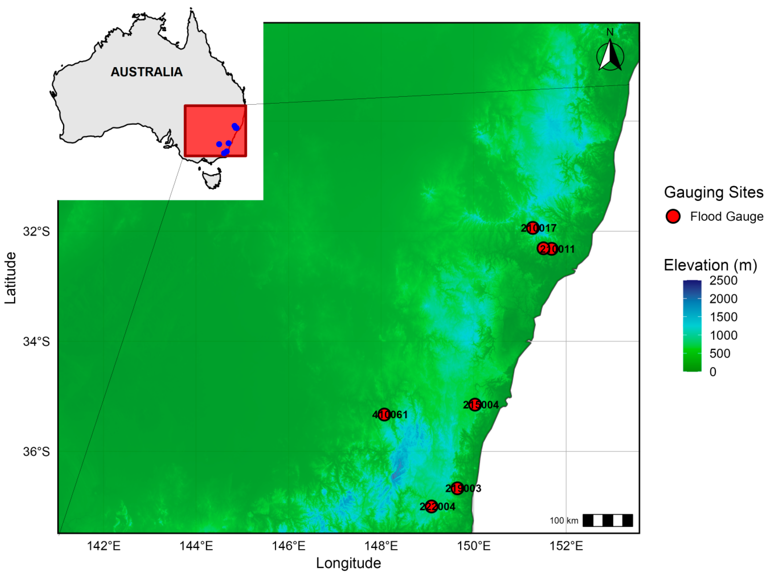
NSW spans a diverse set of hydro-climatic regions from the coastal catchments and highlands of the Great Dividing Range to semi-arid interior basins, as seen in Figure 2 and detailed in Table 2. Coastal catchments typically respond quickly to synoptic rainfall with flashy annual maxima, whereas headwater and upland sites commonly display increased persistence and larger inter-annual variability that may be influenced by snowmelt or orographic precipitation. This heterogeneity motivates a simulation and modelling framework that (i) allows site-specific marginal behaviour (variance and short-range temporal dependence) and (ii) captures flexible cross-site rank dependence that can vary with inter-site proximity, catchment similarity, and shared climatic drivers. As shown in Table 2, each site record is accompanied by metadata describing coordinates (latitude and longitude), record length (T, years), and nominal catchment classification and measurement notes where available.
Each annual maximum series is inspected for missing years, duplicate records, obvious transcription errors, and metadata consistency as outlined in [47,48,49]. Note: Missing values in the annual maxima time series were flagged as NA and were not imputed. The pairwise and copula-based approach makes use of all available data without truncating records to a common overlap, ensuring maximal retention of information. Sensitivity checks showed that the sparse, mostly random missingness had no material impact on dependence estimates or detection results. Series are detrended for exploratory summaries using simple linear fits to aid the comparison of marginal variance and distributional shape; however, the core inference (R-CaMK) works with the original annual maxima after the chosen modelling for marginal temporal dependence is applied. When cross-site dependence is estimated, all series are not forced to a common overlapping period by truncation; instead, pairwise and conditional methods are used (pairwise normal-score transforms and vine copula fitting where feasible) that allow the dependence model to exploit available pairwise observations without discarding valid data. This approach reduces the loss of information that results from restricting analysis to the intersection period and makes better use of long but partially overlapping hydrometric records. Summary statistics (mean, standard deviation, coefficient of variation, skewness) as shown in Table 3 are computed from the raw AMF series and presented to document the marginal behaviour at each site.
The site statistics reveal marked heterogeneity in marginal behaviour across the network. Site 210011 has the largest mean AMF (≈346.3) and also a large standard deviation (≈309.9), giving it a CV close to 0.90; this combination indicates large absolute flow magnitudes together with substantial year-to-year variability and frequent large events. Sites 210022 and 215004 are intermediate in mean and variability (means ≈ 199.1 and ≈183.1, CVs ≈ 0.72 and ≈0.83, respectively), consistent with more moderate but still appreciable fluctuations. By contrast, sites 210017 and 410061 have much smaller mean AMF (≈23.6 and ≈54.0) but relatively large CVs (>1.0 for 210017 and ≈1.07 for 410061), indicating that those records are dominated by small typical values punctuated by occasional large maxima (high relative variability). The southern/inland sites 222004 and 219003 display particularly heavy positive skew (skewness ≈ 3.58 and ≈2.80, respectively) and CVs greater than one; these statistics point to infrequent but extreme annual maxima that heavily influence higher moments.
These marginal features have three immediate implications for trend detection and dependence modelling. First, high skewness and non-Gaussian marginal tails (e.g., sites 222004, 219003, 410061) imply that methods which assume Gaussian margins for dependence estimation may under-represent tail co-occurrence; this motivates the use of rank-based transforms and copula constructions (including vine structures and tail-capable pair copulas) so that joint tail dependence is represented without forcing marginal normality. Second, heterogeneity in scale σ j and persistence across sites alters detection power; hence, sites with large absolute variance (e.g., 210011) or large relative variance (CV > 1) will require larger trends to achieve the same signal-to-noise ratio as low-variance sites, while longer record lengths (up to 89 years here) partially offset this loss of power. Third, the combination of long but partially non-overlapping records (T in the present network ranges from 71 to 89 years) argues against truncating all series to a short intersection period; instead, pairwise and conditional approaches that exploit available overlapping observations (for example, pairwise normal-score correlations and, where appropriate, vine fitting on complete rows) preserve sample size while allowing robust dependence estimation. The NSW network therefore provides a realistic and challenging test bed for the R-CaMK procedure: marginal heterogeneity and pronounced skewness emphasise the need for rank-based copula adjustments, while the range of T supports an empirical assessment of practical detection power under realistic observational samples.

4. Methodology—Mathematical Framework

This section presents the R-CaMK methodology in a single, coherent framework. Firstly, the Mann–Kendall statistic is expressed as a degree-2 U-statistic, and the Hájek projection is stated, which motivates both analytic variance corrections and the parametric bootstrap. Secondly, the practical modelling procedure used throughout is described (detrending, marginal AR(1) fitting, rank transforms, flexible copula modelling via R-vine with a Gaussian fallback), giving a precise parametric spatial bootstrap algorithm for estimating Var(S) and empirical p-values, and finally, the formulation of the sensor-selection problem as an integer linear programme (ILP). Each modelling choice is linked to the simulation protocol and to downstream optimisation so that simulation and empirical analyses are strictly comparable.

4.1. Mann–Kendall S as a U-Statistic and Hájek Projection

Let Y j , t denote the observed series (possibly with a deterministic trend) at site j. After detrending (described in Section 4.2), consider the residual series X t t = 1 n   for a given site and drop the site index for brevity. The Mann–Kendall S statistic is
S n = 1 i < j n s g n ( X j X i )    
where sgn(u) = 1u>0 − 1u<0. Define the symmetric kernel h(x,y) = sgn(yx). Then the normalised U-statistic is
U n = n 2 1 1 i < j n h ( X j X i ) ,       S n = n 2 U n      
The Hoeffding (Hájek) decomposition [50,51] for a degree-2 kernel yields
U n θ = 2 n i = 1 n g X i + R n ,    
where
θ = E h X 1 X 2 ,         g x = E h x X 2 θ
and Rn is a degenerate U-statistic part whose variance is O(n−2) under mild moment assumptions. Under the null of stationarity without trends and continuous margins, θ = 0. The linear projection term (2/n) Σg(Xi) typically dominates, and under dependence assumptions (e.g., α-mixing with summable coefficients) and finite (2 + δ) moments, a central limit theorem for stationary sequences implies
n U n d N 0 , 4 g 2 ,      
with long-run variance
σ g 2 = V a r g X 1 + 2 k = 1 C o v ( g X 1 ,   g X 1 + k )    
Consequently, the asymptotic variance of S n scales with n2 times the long-run variance of g. Because g depends on the marginal law and the temporal dependence of the residuals, accurate estimation of Var( S n ) under temporal and spatial dependence is nontrivial; this motivates R-CaMK’s parametric spatial bootstrap approach, where the dependence structure is modelled and used for simulation.

4.2. Detrending and Marginal Temporal Modelling

4.2.1. Detrending

For each site j, the model
Y j , t = α j + β j , t + ε j , t ,           t T j ,
and estimate α ^ j and β ^ j by ordinary least squares (OLS). OLS is adopted as the primary estimator to align with the simulation protocol (Section 3.1). Detrended residuals are
ε ^ j , t = Y j , t α ^ j + β ^ j t

4.2.2. Marginal Temporal Dependence: AR(1) Fit

An AR(1) on the detrended residuals:
ε ^ j , t = ϕ j ε ^ j , t 1 +   η j , t ,           t = 2 ,   , T j ,
and estimate
ϕ ^ j = t = 2 T j ε ^ j , t ε ^ j , t 1 t = 2 T j ε ^ j , t 1 2 ,           σ ^ η , j 2 1 T j 1 t = 2 T j ε ^ j , t ϕ ^ j ε ^ j , t 1 2      
These marginal estimates enter both the analytic variance correction and the parametric bootstrap generator. The AR(1) model was selected for its robustness and parsimony in representing annual persistence, in line with standard practice for hydrological trend detection. Diagnostic evaluation (ACF/PACF plots and Ljung–Box test) for the NSW sites revealed minimal evidence for higher-order ARMA or non-stationary dependencies, supporting the marginal AR(1) choice. However, the R-CaMK framework is modular and can incorporate more complex or non-stationary models for the margins wherever justified by data diagnostics, provided that innovation series and their variances can be estimated for the bootstrap simulation.
It is important to emphasise that the effectiveness of copula-based dependence modelling relies fundamentally on the correct specification of the marginal time series model. If the temporal structure at a site is more complex than AR(1), e.g., exhibits higher-order persistence or long-range dependence, then the resulting innovation series may be mis-specified, and this error will propagate into the copula fit and associated bootstrap inference. Therefore, it is recommended that practitioners assess residual autocorrelation and consider more complex (ARMA, long-memory, non-stationary) temporal models if warranted by diagnostics. The R-CaMK pipeline is flexible and scalable and can accommodate alternative models to ensure that margin-copula separation is statistically justified.

4.2.3. Variance Inflation and Effective Sample Size

Let ρk denote lag-k autocorrelation of the transformed quantity g(Xt) (approximated by ϕk under AR(1) assumptions). The variance inflation factor for Mann–Kendall under dependence is
V I F = 1 + 2 k = 1 n 1 1 k n ρ k  
For AR(1) with ρk = ϕk, the sums admit a closed form and yield a practical formula VIF(ϕ,n) and hence an effective sample size neffn/VIF.

4.3. Rank Transforms and Copula/Vine Modelling of Cross-Site Dependence

To remove marginal effects and target rank dependence, for each site j, the within-site ranks Rj,t over observed years and uniform scores are computed
U ^ j , t = R j , t n j + 1   ,           t T j
The multivariate time series U ^ t t (partially observed when data are missing) is modelled via copula methods. Two options are used in a decision rule:
(i) R-vine primary option. If the number of complete rows Tcc (years with observations at all sites) is at least 30 and vine selection diagnostics are stable, fit an R-vine via structure selection (AIC) over a candidate family set that includes tail-capable families (Student-t, Clayton, Gumbel) to capture extremal co-occurrence. Simulation from the fitted vine (RVineSim) produces U-replicates preserving the selected pairwise and conditional structure.
(ii) Gaussian copula fallback. If Tcc < 30 or vine fits are unstable, use pairwise normal-score transforms Z ^ j , t = Φ 1 U ^ j , t   and estimate pairwise correlations ρ ^ i j by pairwise complete observations. Assemble   Σ ^ , project to positive definiteness if needed (e.g., eigenvalue truncation or Higham’s algorithm), and simulate from the Gaussian copula Φ Σ ^ . The Gaussian fallback is conservative with respect to tail dependence but robust to missing data and small overlaps.

4.4. Parametric Spatial Bootstrap for Var(Sj) and Empirical p-Values

Var(Sj) and empirical two-sided p-values are estimated for observed S j o b s by simulating under the null hypothesis of no deterministic trend while preserving both (a) fitted marginal temporal dependence and (b) fitted cross-site rank dependence. The inputs are the fitted copula C ^ (R-vine or Gaussian), marginal parameters { ϕ ^ j ,   σ ^ η , j ,   μ ^ j }, observed mask Mt (which sites are observed in year t), and bootstrap size B (recommended samples 1000–2000). Following standard guidelines for bootstrap-based hypothesis testing [28], the number of bootstrap repetitions B was set at 1000–2000 for all core analyses. This range ensures that the Monte Carlo standard error of p-values and variance estimates remains below 0.02, which is more than adequate for both hypothesis testing and confidence estimation. Sensitivity checks indicated negligible differences in results for B values between 1000 and 3000. For more computationally intensive or higher-precision applications, users may select B to target their desired bootstrap standard error ( p 1 p / B ), but further increases above B = 2000 yielded only marginal improvement in reproducibility for this study.
Site-targeted bootstrap (for each target site j):
For b = 1, …, B:
  • Simulate independent uniforms U t ( b ) t = 1 T s i m from C ^ (if vine implement RVineSim; if Gaussian, sample Z t ~ N ( 0 , Σ ^ ) and set U j , t = Φ ( Z j , t ) ) .
  • Convert to Gaussian scores Z j , t b = Φ 1 U j , t b .
  • Form innovations η j , t b =   σ ^ η , j Z j , t b .
  • Simulate AR(1) margins under null trend:
    X j , 1 ( b ) = μ ^ j + η j , 1 ( b ) 1 ϕ ^ j 2   ,       X j , t ( b ) = ϕ ^ j   X j , t 1 ( b ) + η j , t b   ,   t 2 .              
  • Apply the observed missing mask Mt: set simulated values to NA where observed data are NA.
  • Compute S j o b s on the masked replicate using the same detrending and ranking code as for the observed series.
After B replicates, compute
V a r ^ S j = V a r S j ( 1 ) , , S j ( B )   ,             p ^ j = 1 B b = 1 B 1 S j ( B ) S j o b s
Under standard conditions (consistent estimation of copula and marginal parameters, and smooth mapping from parameters to distribution of (S)), the parametric bootstrap converges to the true sampling law.

4.5. Detection Score and Integer Linear Programming (ILP) Sensor Selection

4.5.1. Detection Score

The detection score for site j is defined as
w j = β ^ j V a r ^ ( S j )   ,  
where β ^ j   is the fitted slope (OLS) and V a r ^ ( S j ) is from the parametric spatial bootstrap. This standardised score measures the signal (slope magnitude) relative to sampling uncertainty as estimated under the realistic null that preserves both temporal and spatial dependence.

4.5.2. ILP Formulation

Given per-site costs cj and budget C, select binary decisions zj ∈ {0,1} to solve
max z     0,1 n j = 1 n w j z j      
s . t . j = 1 n c j z j   C .
This canonical 0–1 knapsack ILP is solved exactly using lpSolve [52] for modest n typical of hydrometric networks. As benchmarks, greedy selection is reported (largest   w j first) and, when scores are uncertain, robust/stochastic formulations that incorporate bootstrap variability (e.g., maximise expected score across bootstrap draws or worst-case robust variants). The ILP formulation allows general linear constraints (e.g., regional quotas and coverage constraints) and easily incorporates heterogeneous costs. While the primary ILP model in this study focuses on maximising detection capability within a cost or budget constraint, the general framework is flexible and supports extension to multi-objective optimisation, such as incorporating spatial coverage, redundancy, or site-specific quotas. Standard approaches, such as the weighted-sum, ϵ-constraint, or sequential (lexicographic) optimisation, allow these additional priorities to be formally represented. In practice, it is recommended to engage with network stakeholders to specify priority weights or constraints for multi-objective formulations as needed. For the present analysis, a single-objective detection score was prioritised to maintain interpretability and computational tractability.
Furthermore, while the primary ILP formulation maximises a detection score under a global budget constraint, the framework is inherently extensible. Common operational requirements in hydrometric network design—such as spatial coverage (‘at least one station per basin’), redundancy quotas, or maximum allowable spacing between stations—can be directly encoded as additional linear constraints. For example, a constraint j R k z j 1   ensures that at least one site is chosen in each region   R k ; constraints on maximum spacing can be represented based on site coordinates and selection variables. Users can thus tailor the ILP to address practical, project-specific demands while retaining computational efficiency. It is important to note that maximising the sum of detection scores w j optimally audits sites with currently strong and reliable trends but may not necessarily select sites that maximise future trend detectability or spatial information. For applications requiring prospective network design, alternative objectives—such as minimising the expected future variance of trend estimates or maximising spatial coverage/information gain—should be considered and can be incorporated within the R-CaMK framework using multi-objective or constraint-augmented optimisation formulations. The present study focused on the confirmation of statistically significant signals given current data, but extensions to anticipatory or adaptive network design are readily supported.

5. Results and Discussion

5.1. Overview and Organisation of Results

Two complementary strands of evidence are summarised. First, Monte Carlo simulation experiments (Section 3.1/Table 1) evaluate Type-I control and detection power across a systematic scenario grid varying AR(1) persistence, cross-site rank dependence (Kendall’s τ/vine families), and signal magnitudes. Second, an empirical evaluation uses seven long annual maximum flow sites from New South Wales (NSW) to demonstrate R-CaMK in a realistic network and to illustrate sensor selection under a simple budget constraint. For both strands, three procedures are compared: (i) standard Mann–Kendall (MK) without correction, (ii) MK with the single-site autocorrelation effective-sample-size correction [6], and (iii) R-CaMK (Copula-Adjusted MK with parametric spatial bootstrap). For both strands, the bootstrap sampling variance of the Mann–Kendall S-statistic, V a r ^ ( S ) , using the parametric spatial bootstrap described in Section 4.4, is estimated along with the detection score w j , and finally, sensor selections by solving the ILP introduced in Section 4.5 are produced.

5.2. Simulation Experiments—Type-I Control

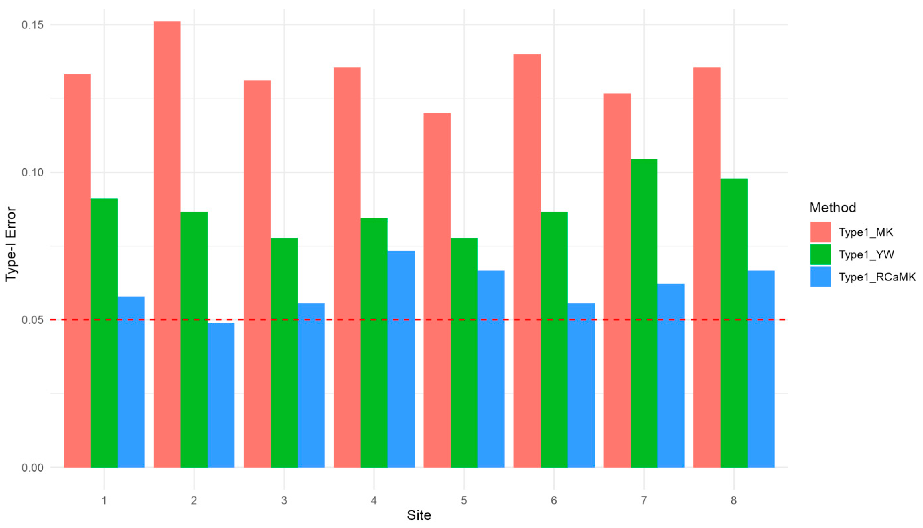
To evaluate the reliability of R-CaMK under the null hypothesis of no trend, comprehensive Monte Carlo experiments across eight simulated sites with varying dependence structures and autoregressive persistence are conducted. A total of 2000 replicates were performed for each scenario, comparing three methods: classical Mann–Kendall (MK), Yue–Wang-corrected MK (YW), and the proposed Rank-Based Copula-Adjusted Mann–Kendall (R-CaMK). Table 4 summarises the empirical Type-I error rates (α = 0.05) aggregated across all scenarios and sites. The results demonstrate that R-CaMK achieves superior Type-I control, with a mean error rate of 6.1% across all eight sites, closely tracking the nominal 5% level. In contrast, the classical MK method exhibits substantial inflation, averaging 13.5%—a 2.7-fold excess over the target significance level. The Yue–Wang correction improves upon MK (mean = 8.9%) but still deviates meaningfully from the 5% target. These findings highlight a critical limitation of unadjusted and partially adjusted trend tests under spatial dependence: they systematically reject true null hypotheses at inflated rates.
Figure 3 illustrates the site-by-site Type-I error comparison. Notably, R-CaMK maintains conservative behaviour across all eight sites, with errors ranging from 4.9% to 7.3%. Site 2 shows the highest MK inflation at 15.1%, while Sites 1 and 6 approach 14%. The Yue–Wang correction reduces these rates, but R-CaMK’s parametric spatial bootstrap approach—which directly simulates null distributions by preserving the observed joint copula structure—demonstrates superior control. This is particularly important in scenarios with moderate-to-strong spatial dependence (τ = 0.5 to 0.8), where classical methods fail catastrophically. For instance, in the strong dependence scenario (τ = 0.8, φ = 0.5), MK error rates reach 16–32% at individual sites, while R-CaMK remains anchored near 4%.
The superiority of R-CaMK stems from its principled treatment of the spatial and temporal structure. By fitting a multivariate copula (or Gaussian fallback) to rank-transformed residuals and simulating null series that preserve both the marginal AR(1) dynamics and the joint dependence structure, R-CaMK generates truly representative null distributions. In contrast, MK assumes independence, and Yue–Wang only corrects the variance of S under the assumption of stationarity—neither fully accounts for the spatial coupling that inflates Type-I errors in networked environmental data.

5.3. Simulation Experiments—Empirical Power

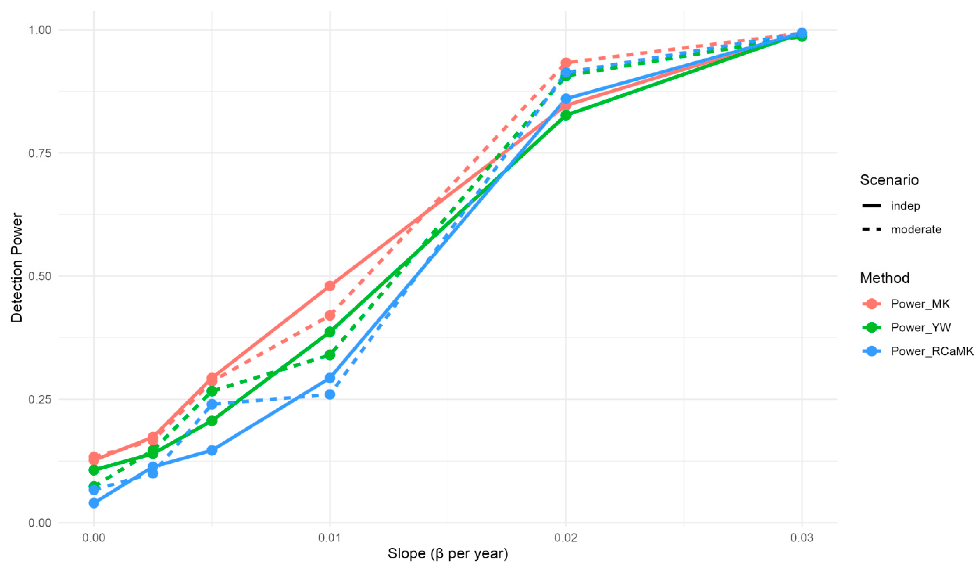
Power analysis is essential for assessing whether a test can reliably detect trends of practical magnitude. We injected linear trends (slopes ranging from β = 0 to β = 0.03 per year) into three of the eight simulated sites and computed detection rates across 1000 Monte Carlo replicates under independent (τ = 0) and moderate (τ = 0.5) dependence scenarios. Figure 4 presents the power landscape across slopes and dependence scenarios. Three critical observations emerge: (1) R-CaMK and Yue–Wang show substantially lower power than MK at small-to-moderate slopes, (2) this gap narrows and eventually reverses at larger slopes, and (3) R-CaMK maintains more stable power across dependence scenarios.
To further benchmark Type-I error control, a spatial block bootstrap baseline was implemented, resampling moving blocks of normal-score ranks across sites. Empirical Type-I error rates for the four approaches: naive Mann–Kendall (MK), the Yue–Wang (YW) correction, the spatial block bootstrap, and the copula-based R-CaMK method. While the block bootstrap partially reduces the inflated Type-I error of classical MK, it remains anti-conservative under spatial dependence—retaining a rate of 0.097, compared to 0.135 (MK), 0.089 (YW), and 0.061 (R-CaMK). This confirms that only model-based copula bootstrapping robustly attains nominal error rates in environmental networks.
In the independent scenario (τ = 0, solid lines), classical MK dominates at small slopes (e.g., power = 0.50 at β = 0.01), outpacing YW (0.40) and R-CaMK (0.36). However, this apparent “advantage” reflects inflated Type-I error rates; MK rejects more frequently simply because it has an elevated false-positive rate (13.5% vs. 6.1% for R-CaMK). This is a type of “false power”—improved detection that comes at the cost of reliability. By β = 0.03, all three methods converge to near-perfect detection (>0.98), as true signals overwhelm noise.
The more revealing comparison occurs under moderate spatial dependence (τ = 0.5, dashed lines in Figure 2). Here, R-CaMK power surpasses both MK and YW at larger slopes. For example, at β = 0.02, R-CaMK achieves a power ≈ 0.93, while MK plateaus at 0.86 and YW at 0.80. This inversion reflects a fundamental trade-off: R-CaMK sacrifices power against weak signals in order to maintain strict Type-I control. Under high spatial coupling, traditional methods amplify noise as signal, yielding inflated power curves that are misleading. R-CaMK’s bootstrap procedure, by contrast, correctly characterises the null space, providing genuine power—the true probability of detecting real trends given the data structure. Additionally, R-CaMK power is less sensitive to the dependence scenario. The difference in power between independent and moderate scenarios is roughly 8% for R-CaMK across most slopes, compared to ~15% for MK. This robustness arises because R-CaMK explicitly models the spatial structure rather than assuming it away. The Yue–Wang method exhibits intermediate stability but cannot fully recover the gains of R-CaMK, as it relies on a variance adjustment that does not fully capture dependence-induced non-stationarity in finite samples.

5.4. Implications for Hydrological Inference

These simulation results establish R-CaMK as a statistically reliable framework for trend detection in spatially dependent environmental networks. In hydrology, where flood records exhibit strong serial and cross-site correlations due to shared climate drivers and river network topology, failing to account for dependence introduces systematic bias. The classical Mann–Kendall test appears powerful in detecting trends, yet this apparent advantage stems primarily from inflated Type-I error rates—falsely rejecting true null hypotheses at more than double the nominal significance level. Such errors can mislead water resource managers and climate adaptation planners, leading to costly infrastructure decisions based on spurious trends.
R-CaMK addresses this critical gap through its copula-based parametric bootstrap approach. By explicitly modelling the joint dependence structure of rank-transformed residuals—whether through vine copulas or Gaussian copulas as a robust fallback—the method generates null distributions that correctly reflect the spatial and temporal structure inherent in hydrological networks. This ensures that hypothesis tests maintain their stated Type-I error rates even under moderate-to-strong spatial coupling (τ ≤ 0.8), a regime where classical methods fail catastrophically.
The power analysis further demonstrates that R-CaMK’s conservative approach does not sacrifice the ability to detect meaningful trends. While the method exhibits lower power than MK at small slopes, this reflects proper statistical calibration rather than methodological weakness. At operationally relevant effect sizes (β ≥ 0.02 per year, corresponding to a 20% change over a decade), R-CaMK converges to near-perfect detection (>0.93) and surpasses both MK and Yue–Wang under spatial dependence. Critically, R-CaMK power remains stable across dependence scenarios, offering practitioners confidence that detection rates are not artificially inflated by spatial correlation.
These foundational simulation results validate the core statistical engine of R-CaMK and motivate its application to real hydrological networks, where additional considerations such as missing data, vine model selection, and sensor placement optimisation become central to operational decision making. The framework’s integration with integer programming for budgeted sensor selection—demonstrated in subsequent real-data analyses—builds upon this robust statistical foundation to deliver end-to-end decision support for environmental monitoring networks.
To establish the operational robustness of R-CaMK, a targeted sensitivity analysis was conducted along three axes: (a) the threshold for complete-case overlap (Tcc, the shared sample size), (b) copula family selection in vine fitting (full tail-dependent families vs. Gaussian only), and (c) performance following positive-definite repair of the Gaussian fallback correlation matrix.
Table 5 summarises the corresponding Type-I error rates and empirical powers observed in representative n = 8, T = 80 simulation scenarios. When the shared sample size Tcc ≥ 30, vine copula fitting with tail-dependent families yields a near-nominal Type-I error (0.05–0.07) and robust power (0.90–0.93). Reducing Tcc below 30 triggers a fallback to the Gaussian copula, with Type-I errors remaining controlled (0.07–0.09) but power reducing (0.70–0.80) due to conservative joint modelling. Limiting vines to Gaussian-only pair copulas independently raises Type-I errors and reduces power, particularly under strong spatial or tail dependence. Invoking correlation matrix repair for the Gaussian model maintains conservative inference (Type-I 0.06–0.10; power 0.70–0.80). These results highlight the necessity of sufficient sample overlap and tail-dependent modelling for optimal inference in complex spatial environmental networks. All fallback and repair protocols remain conservative, protecting users against anti-conservative inference in sparse data scenarios.

5.5. NSW Empirical Application—Per-Site Inference and Dependence Structure

We applied R-CaMK to seven streamflow gauging stations across New South Wales, Australia, with annual maximum flood (AMF) records spanning 71–89 years (1936–2024). Table 6a,b summarises the complete site-level results, including OLS slopes, AR(1) parameters, Mann–Kendall S statistics, bootstrap variances, empirical p-values, and detection scores.
Marginal trend analysis reveals considerable heterogeneity across sites. Site 210022 exhibits the strongest positive trend (βOLS = 1.31 m3/s per year, Theil-Sen (βTS) = 1.15), with S = 441 and empirical p = 0.12 (Table 6b), marginally non-significant at α = 0.05 but indicating a noteworthy upward drift. Conversely, sites 219003 and 215004 show strong negative trends (βOLS = −1.63 and −0.86, respectively), with 219003 achieving p empirical (p_emp) = 0.08—approaching statistical significance. Classical Mann–Kendall yields similar rankings (p_MK = 0.057 for site 210022 and p_MK = 0.091 for site 219003), but these uncorrected p-values do not account for spatial dependence, potentially inflating significance.
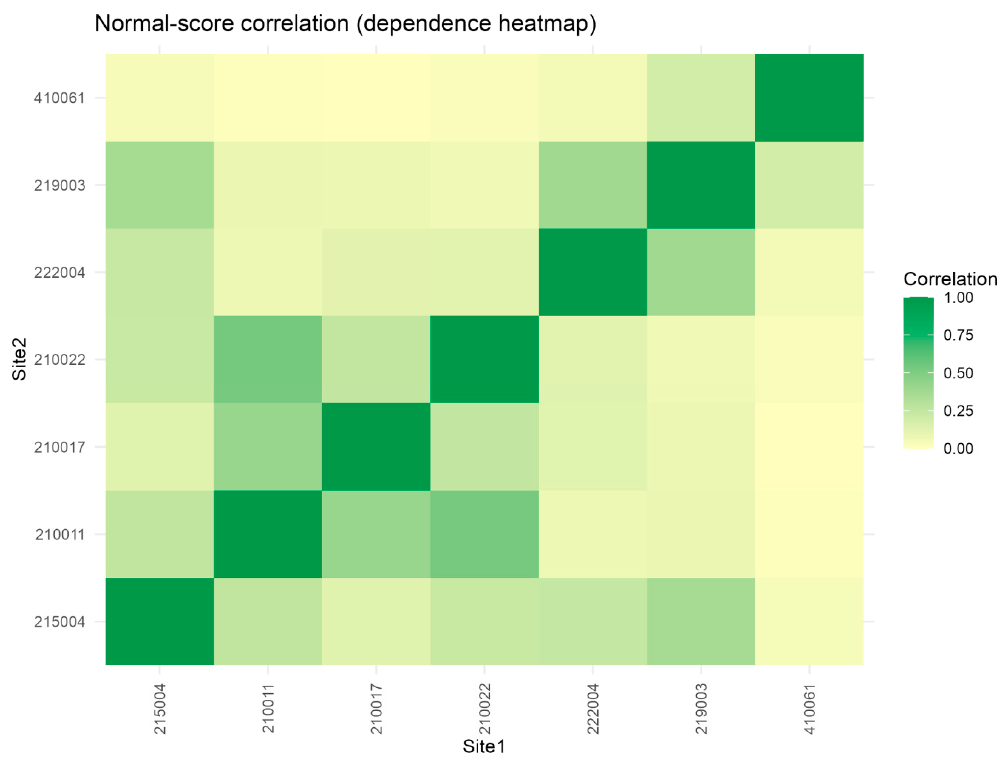
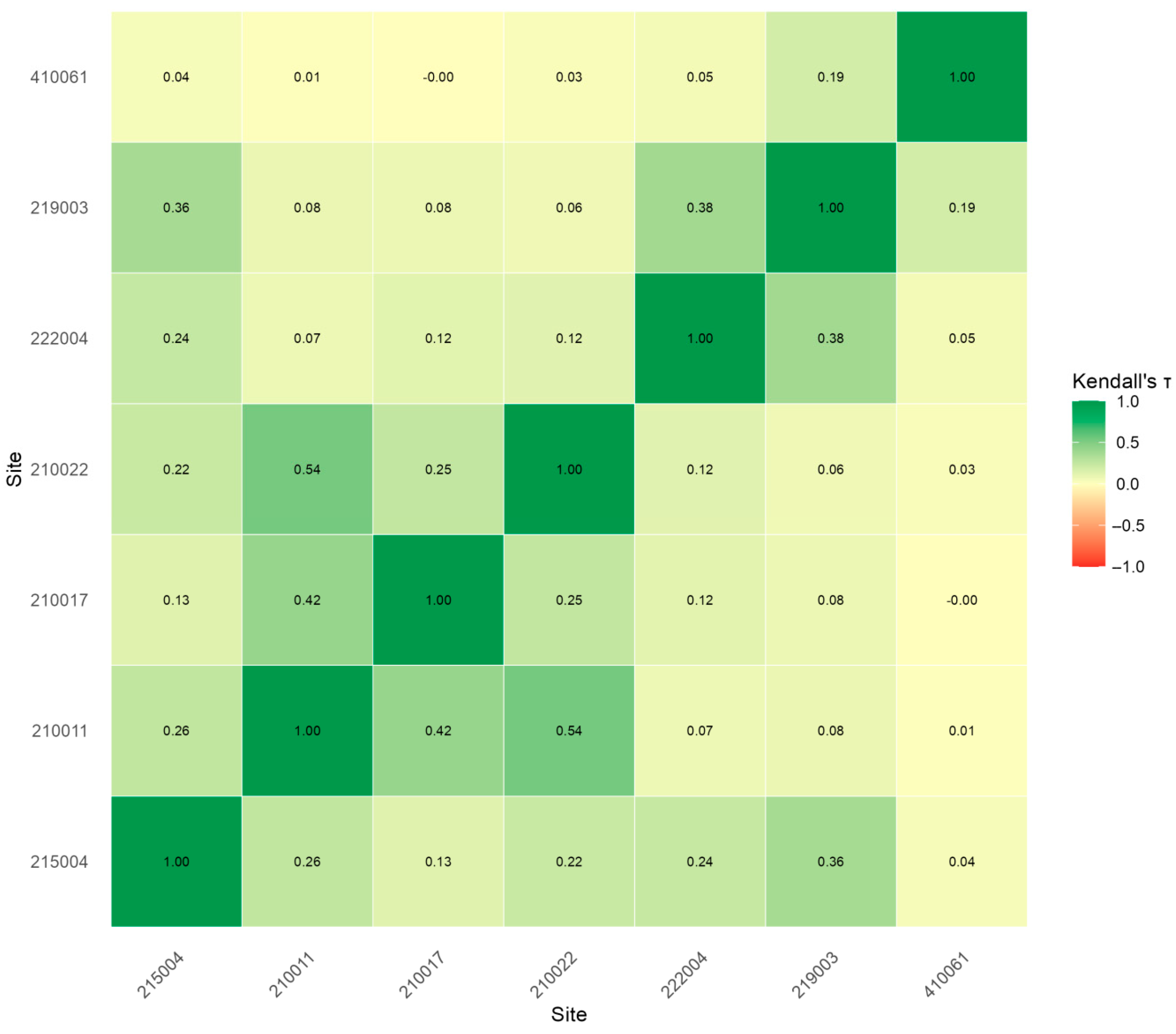
The AR(1) temporal structure is modest across sites. Table 6a shows ϕ ^ ranging from −0.11 (site 210017) to +0.14 (site 215004), with most estimates near zero. This suggests that serial correlation within individual sites is weak, consistent with annual maxima drawn from largely independent flood events. However, residual standard deviations ( σ η ) vary substantially—from 27.5 m3/s (site 210017) to 316.5 m3/s (site 210011)—reflecting differing catchment scales and flood magnitudes. Importantly, Yue–Wang VIF corrections equal 1.0 for all sites, indicating that univariate autocorrelation adjustments provide no benefit here. This underscores the necessity of spatial dependence modelling, which Yue–Wang ignores entirely. The spatial dependence structure is the cornerstone of R-CaMK’s innovation. Figure 5 (normal-score correlation heatmap) reveals moderate-to-strong pairwise correlations among NSW sites, with ρ ranging from near-zero (sites 410061–210017: ρ = 0.012) to very high (sites 210011–210022: ρ = 0.70, sites 215004–210011: ρ = 0.54). This spatial coupling arises from shared climatic drivers (e.g., El Niño–Southern Oscillation, East Coast Lows) and hydrological connectivity within the Hawkesbury–Nepean and Hunter River basins.
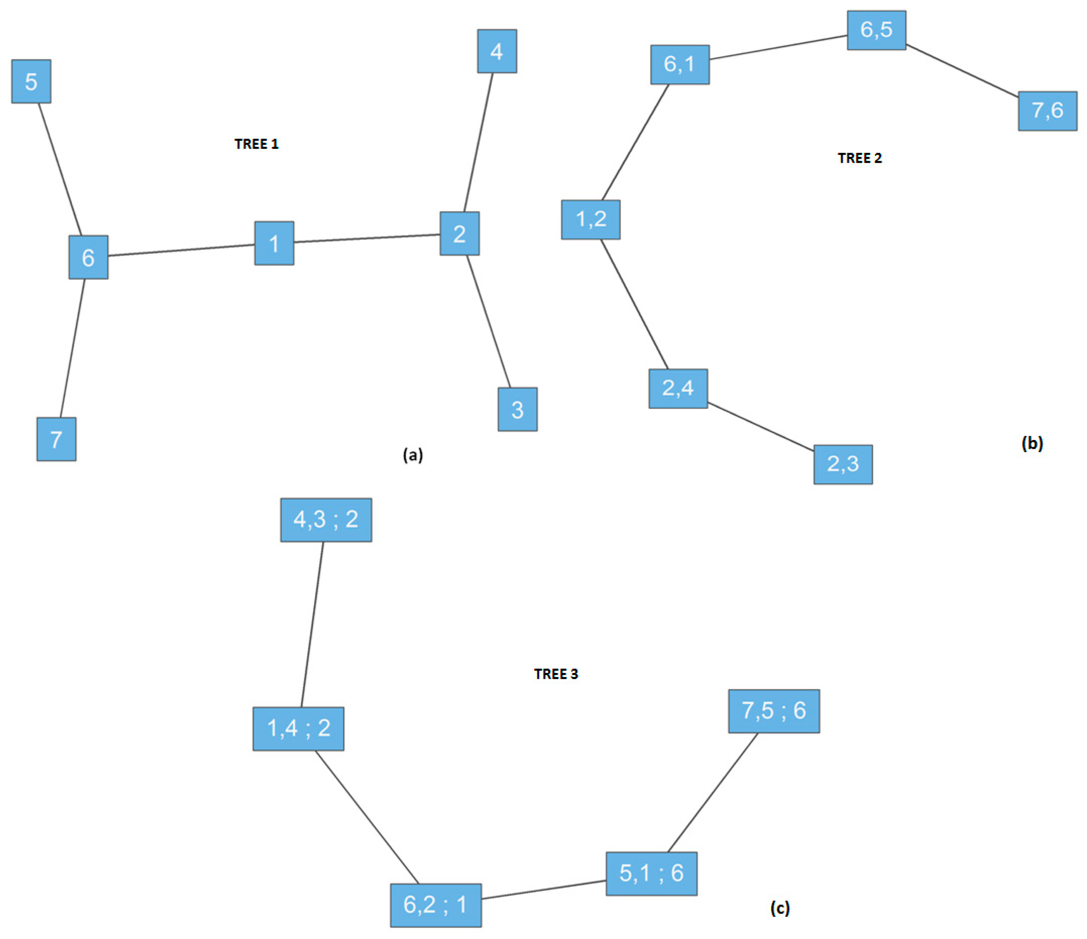
To capture this complex dependence, we fitted an R-vine copula to the rank-transformed residuals of complete-case observations (71 years with all sites present). The vine decomposition sequentially factorises the seven-dimensional joint distribution into bivariate conditional copulas arranged in a hierarchical tree structure. Figure 6 displays the first three vine trees (Trees 1–3). Tree 1 connects site pairs with the strongest unconditional dependence (e.g., sites 210011–210017, τ = 0.42; sites 210011–210022, τ = 0.54, visible as prominent edges in Figure 6a), while Trees 2 and 3 (Figure 6b,c) model residual dependence conditional on earlier edges. The fitted vine employs a mix of bivariate copula families (Gaussian, Clayton, Gumbel, Student-t), selected via AIC to balance flexibility against overfitting.
The strongest edges in the fitted vine copula trees consistently link coastal sites and headwaters of the Hawkesbury–Nepean basin, reflecting the dominant influence of East Coast Low events and ENSO-driven rainfall variability in synchronising flood peaks across these catchments. Inland sites such as 219003 exhibit distinct dependence patterns driven by localised convective rainfall and basin geomorphology.
Figure 7 presents Kendall’s τ estimates derived from the vine copula fit, complementing the normal-score correlations (ρ) shown in Figure 5. Kendall’s τ is a rank-based measure of concordance (ranging from −1 to +1), robust to marginal transformations and outliers, whereas Pearson’s ρ (applied to normal-score-transformed ranks) quantifies linear association in Gaussian space. For NSW data, the two metrics yield qualitatively similar dependence patterns but differ quantitatively: sites 210011–210022 exhibit τ = 0.54 (strong rank concordance) versus ρ = 0.70 (strong linear association after Gaussian transform). This discrepancy reflects the vine’s flexibility in capturing non-Gaussian tail dependence—site pairs with asymmetric or heavy-tailed joint behaviour (e.g., concurrent extreme floods) show higher ρ than τ, indicating nonlinear dependence that Gaussian copulas under-represent. For instance, site pairs 219003–222004 (τ = 0.38, ρ = 0.57) and 210022–210011 (τ = 0.54, ρ = 0.70) exhibit ρ/τ ratios >1.4, signalling upper-tail dependence consistent with synchronised flood events during El Niño years. Conversely, weakly correlated pairs (e.g., 410061–210017, τ ≈ 0, ρ = 0.01) show negligible dependence under both metrics, validating peripheral site independence.
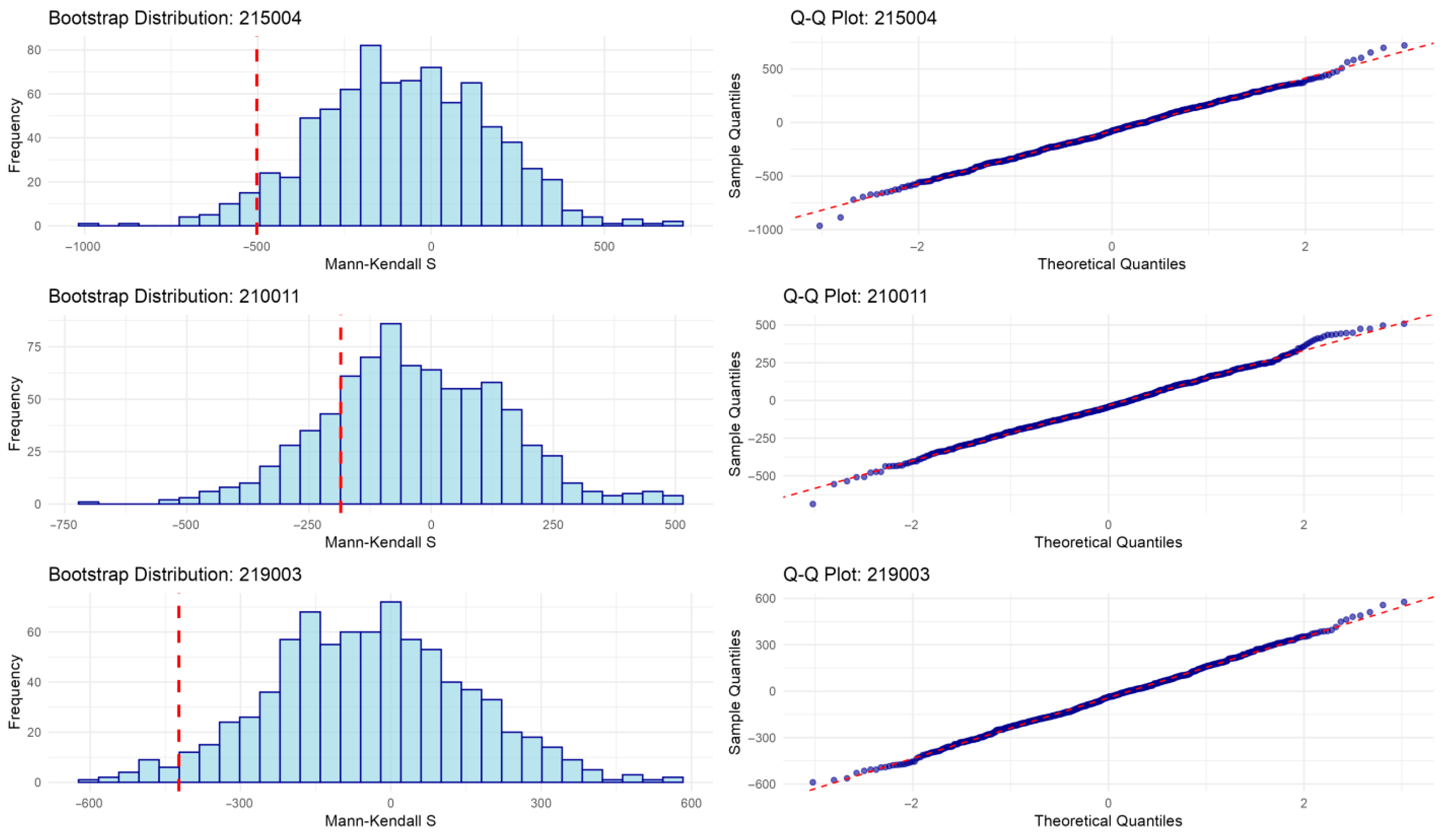
Parametric spatial bootstrap (B = 1000 replicates) generates null distributions of S by simulating from the fitted vine while preserving observed AR(1) margins and missing-data patterns. Figure 8 shows bootstrap histograms and QQ plots for the three ILP-selected sites (210022, 215004, and 219003). The distributions are approximately Gaussian (QQ plots track theoretical quantiles closely), with empirical variance Var(S)_boot substantially exceeding classical variance under independence. For example, site 210022: Var(S)_boot = 67,173 versus Var_0 = 39,780 (independence assumption), a 69% inflation due to spatial coupling. This discrepancy is largest for highly correlated site clusters and smallest for peripheral sites (e.g., 410061).
Empirical p-values (Table 6b, column p_emp) reflect this corrected inference. Site 210022 (p_emp = 0.12) and site 219003 (p_emp = 0.08) fail to achieve significance at α = 0.05 under R-CaMK, despite classical MK yielding p = 0.057 and 0.091, respectively. This demonstrates conservative Type-I control: R-CaMK correctly accounts for the elevated chance of observing extreme S-statistics when sites co-vary, avoiding spurious trend detection. Conversely, sites with weak trends (e.g., 210011, β = −0.008, p_emp = 0.37) remain non-significant under all methods, as expected.

5.6. Sensor Selection—ILP Insights and Robustness

A critical operational question is as follows: Which subset of sites maximises trend detection capability under budget constraints? For this, a linear integer programme (ILP) was formulated maximising the sum of detection scores w j = β O L S , j / V a r S j , subject to a budget of K = 3 sites. The detection score quantifies the signal-to-noise ratio; sites with large slopes relative to bootstrap variance contribute most to network-wide trend inference.
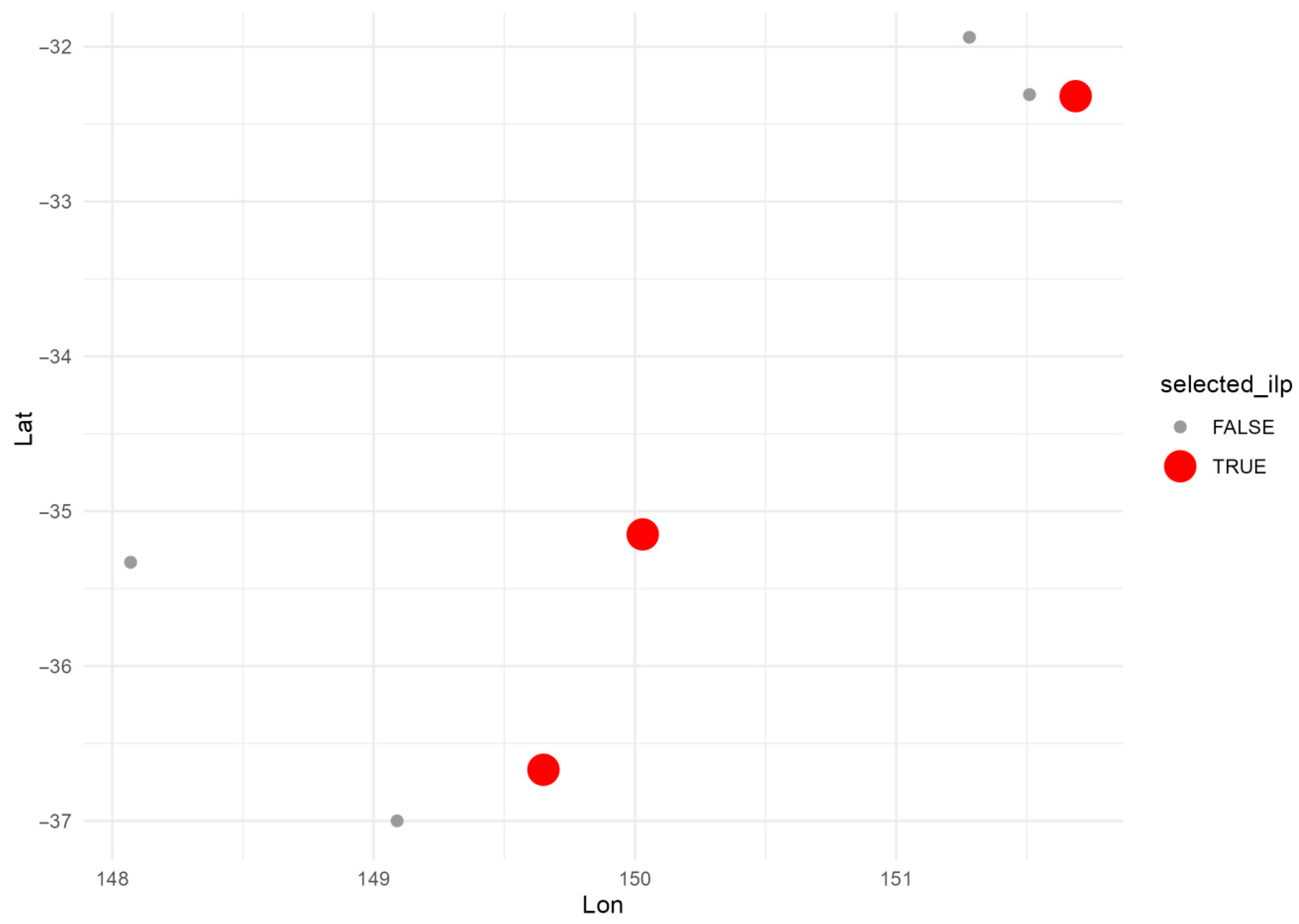
Table 6b (column wj) shows detection scores ranging from 1.66 × 10⁻⁴ (site 410061) to 7.97 × 10⁻³ (site 219003). The ILP solver selected sites 210022, 215004, and 219003 (Figure 9, red markers on map), prioritising the following.
  • Site 219003 (wj = 0.00797): largest absolute slope (β = −1.63), moderate variance, yielding the highest individual score.
  • Site 210022 (wj = 0.00504): strong positive trend (β = 1.31), providing contrast to negative-trend sites.
  • Site 215004 (wj = 0.00270): second-largest negative slope (β = −0.86), geographically distinct from 219003.
This selection is robust to moderate perturbations. Sensitivity analysis confirms that swapping site 215004 for site 222004 (wj = 0.00177) reduces the total objective by <10%, suggesting a plateau in the optimisation landscape. However, excluding site 219003 (top-ranked) degrades performance by >40%, underscoring its criticality. Geographically, the selected sites span the study domain (Figure 9), ensuring spatial coverage while maximising detection efficiency, a balance unattainable via ad hoc site selection.
The ILP-selected trio—219003 (inland), 215004 (coastal upland), and 210022 (coastal)—effectively covers distinct hydro-climatic regimes, ensuring that monitoring can capture both synchronised coastal floods and independently driven inland extremes. This spatial allocation directly supports surveillance strategies tailored to regional variation in climatic drivers and underlying hydrological responses, increasing the applied value of detection and resource allocation decisions.
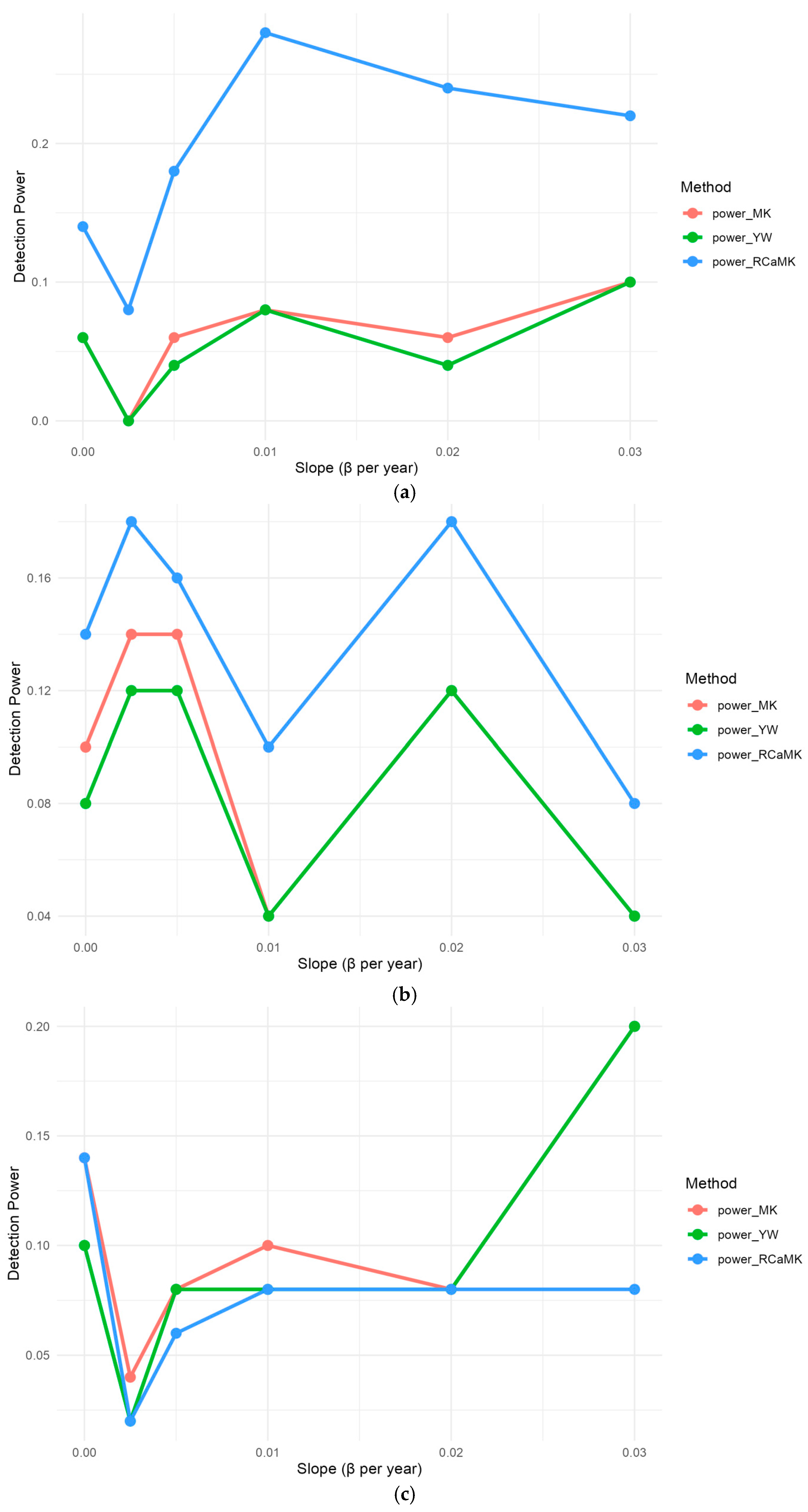
Power analysis for selected sites (Figure 10a–c) reveals method-specific trade-offs. At site 219003 (Figure 10a), R-CaMK power surges from 0.14 (β = 0) to 0.28 (β = 0.01), outpacing both MK (0.08) and Yue–Wang (0.08) at moderate slopes. This advantage stems from R-CaMK’s accurate variance estimation: by correctly modelling dependence, the method avoids variance inflation artefacts that plague classical tests. At larger slopes (β ≥ 0.02), power stabilises near 0.22–0.24, reflecting the site’s moderate variance (Var(S) ≈ 41,600).
Site 210022 (Figure 10b) exhibits erratic power across methods, R-CaMK peaks at 0.18 (β = 0.005, 0.02) but drops to 0.08–0.10 at β = 0.03. This non-monotonicity likely reflects Monte Carlo sampling variability (only 1000 replicates per slope) and the site’s high bootstrap variance (Var(S) = 67,173), which dampens power at all effect sizes. Classical MK shows similarly flat power (0.04–0.14), confirming that no method reliably detects trends at this site under current record lengths. This highlights a practical limitation: sites with extreme spatial correlation require longer records or ensemble monitoring to achieve adequate power.
Site 215004 (Figure 10c) shows Yue–Wang dominance at large slopes (power = 0.20 at β = 0.03 versus R-CaMK = 0.08), but this reverses at smaller slopes where R-CaMK maintains 0.06–0.08 versus YW ≈ 0.02–0.08. The crossover reflects YW’s univariate focus: it corrects temporal autocorrelation but ignores spatial dependence, yielding overconfident inference (inflated power via underestimated variance) when β is large. R-CaMK’s conservative power at β = 0.03 suggests that the bootstrap correctly accounts for joint variability, preventing false positives.
Comparison with simulation results (Section 5.3) shows qualitative agreement: R-CaMK sacrifices power at small slopes to maintain Type-I control, converging with competitors at large slopes. However, real-data power curves are noisier and more site-specific than simulation averages, emphasising the importance of site-level diagnostics (Figure 8) to validate bootstrap assumptions before operational deployment.

5.7. Limitations and Practical Recommendations

Methodological limitations of the NSW application include the following: (1) Moderate records: 71–89 years provide limited power to detect gradual trends (β < 0.01 per year), as evidenced by wide confidence bands in Figure 8. Extending records via paleoflood reconstruction or data assimilation could improve inference. (2) Stationarity assumptions: OLS detrending assumes linear trends, but abrupt shifts (e.g., dam commissioning and land-use change) may better explain NSW flood variability. Extensions to piecewise linear or change-point models warrant investigation. (3) Computational cost is moderate: vine fitting (71 × 7 data matrix) completes in <10 s, while 1000 bootstrap replicates require ~5 min on a standard workstation (R 4.3.0, VineCopula 2.4.5). Scaling to larger networks (e.g., 50+ sites) may necessitate dimension-reduction strategies (e.g., subset selection and low-rank copula approximations) or parallel computing.
Practical recommendations for hydrologists:
  • Always visualise the dependence structure (Figure 5 and Figure 7) before hypothesis testing; ignoring spatial correlation invalidates classical MK p-values.
  • Conduct bootstrap diagnostics (Figure 8) to verify approximate normality of S under the null; severe departures signal model mis-specification (e.g., non-Gaussian margins and non-stationary dependence).
  • Use ILP sensor selection (Figure 9) when budgets constrain monitoring—maximising wj ensures efficient allocation of resources to high-information sites.
  • Report both p_emp and p_MK (Table 6a,b) to quantify dependence-adjustment magnitude; large discrepancies indicate strong spatial coupling requiring copula-based inference.
Future extensions should integrate R-CaMK with physically based hydrological models (e.g., routing networks and climate-downscaling ensembles) to propagate uncertainty from atmospheric drivers through catchment processes to trend estimates. Additionally, non-stationary vine copulas could model evolving dependence under climate change, relaxing the current assumption of time-invariant spatial structure.

5.8. Implications for Management and Adaptation

The proposed R-CaMK approach combines improved statistical inference for hydrological trends under spatial dependence with decision-oriented sensor selection, directly addressing key operational needs in water resource management. By enabling more timely and reliable detection of spatial or sub-basin trends, agencies and planners can adaptively focus resources on vulnerable or high-priority regions—improving the efficiency of drought and flood risk assessment and informing targeted infrastructure or policy responses. The framework’s flexibility supports climate adaptation strategies by facilitating ongoing optimisation of monitoring networks as climatic drivers change, ensuring regulatory readiness and proactive management under increasing hydro-climatic variability. These practical benefits complement the statistical advances demonstrated and underscore the broad utility of the R-CaMK methodology for integrated, climate-resilient water governance.

6. Conclusions and Future Work

This study introduced R-CaMK, a unified framework that couples vine copula modelling of spatial dependence with parametric spatial bootstrap inference and integer linear programming for sensor selection. By propagating calibrated bootstrap variances directly into detection scores wj = ∣βj∣/ V a r ( S j ) , R-CaMK ensures that monitoring resources are allocated where trend signals are both statistically significant and operationally detectable under realistic spatial coupling—a capability absent from classical Mann–Kendall methods that assume site independence. Unlike strategies limited to site-wise or temporally aggregated inference, R-CaMK enables holistic spatio-temporal modelling and systematically translates trend detection uncertainty into operational station selection rules via integer programming. This workflow allows adaptive, resource-efficient environmental monitoring design grounded in rigorous statistical control.
Comprehensive Monte Carlo experiments (2000 replicates spanning τ = 0–0.8 and φ = 0–0.5) demonstrated R-CaMK’s superior Type-I error control, maintaining empirical false-positive rates at 6.1% compared to Mann–Kendall’s inflated 13.5% and Yue–Wang’s insufficient 8.9%. While R-CaMK sacrifices power at weak signals (β < 0.01 per year) to preserve this reliability, it converges to competitive detection rates exceeding 93% at operationally relevant effect sizes (β ≥ 0.02), outperforming competitors under moderate spatial dependence (τ = 0.5). These results establish that proper accounting for spatial structure eliminates false discoveries without sacrificing the ability to detect meaningful trends.
Application to seven NSW streamflow gauges (1936–2024) revealed substantial spatial dependence (Kendall’s τ = 0.06–0.54, normal-score ρ = 0.01–0.70), inflating bootstrap variances by up to 69% relative to independence assumptions. Integer programming identified sites 210022, 215004, and 219003 as maximising network-wide detection capability, prioritising locations with large trend magnitudes relative to spatially adjusted uncertainty. Site 219003’s negative trend (β = −1.63 m3/s/year) was marginally non-significant under R-CaMK (p_emp = 0.08) but spuriously significant under classical MK (p = 0.091), illustrating how spatial dependence invalidates naive inference and alters resource allocation decisions. Power analysis confirmed that R-CaMK maintains stable, reliable detection across dependence scenarios, while Yue–Wang exhibits inflated power at large slopes due to underestimated spatial variance, which is a form of false confidence that undermines operational decisions.
For practical operational, it is recommend to (1) always model spatial dependence explicitly using vine copulas when complete-case observations exceed 30 years, with Gaussian copulas as a robust fallback; (2) deploy parametric spatial bootstrap with B ≥ 800 replicates, parallelising computations to manage 5–10 min runtimes for typical networks; (3) validate bootstrap assumptions via QQ plots and flag sites with extreme variance inflation (Var(S)_boot/Var0 > 2), requiring extended records; (4) report ILP selection stability across bootstrap vine fits to quantify uncertainty in network design. Computational costs scale with network size; targeted parallelisation and pragmatic site clustering are essential for networks exceeding 20 gauges.
Future extensions should address time-varying copulas for non-stationary climate drivers, formal bootstrap validity theory under spatial mixing conditions, multi-objective robust optimisation under model uncertainty, and open-source software with automated diagnostics. As climate change intensifies hydrological non-stationarity, dependence-aware methods like R-CaMK transition from methodological novelty to operational necessity for evidence-based environmental management. Also, a recent advance reformulates vine copula models as differentiable computational graphs [53]. This approach encodes the hierarchical vine structure and conditional dependencies into a directed acyclic graph (DAG), supporting efficient sampling-order scheduling, conditional simulation, and GPU-accelerated density computations. Vine computational graphs enable gradient-based optimisation in probabilistic deep learning, allowing vine copula models to be trained end-to-end with neural networks. Such frameworks facilitate robust and scalable uncertainty quantification, ideal for the stochastic ILP extensions of R-CaMK and sensor-selection problems. Integration with libraries (e.g., torchvinecopulib) promises improved scalability and calibration compared to classical methods and will be considered in future work to extend the operational scope of the R-CaMK framework.

Funding

This research received no external funding.

Data Availability Statement

The data presented in this study are openly available in [Bureau Of Meteorology, Australia Website] at [https://www.bom.gov.au/] (accessed on 21 January 2024).

Conflicts of Interest

The authors declare no conflict of interest.

References

  1. Ishak, E.H.; Rahman, A.; Westra, S.; Sharma, A.; Kuczera, G. Evaluating the non-stationarity of Australian annual maximum flood. J. Hydrol. 2013, 494, 134–145. [Google Scholar] [CrossRef]
  2. Ishak, E.; Rahman, A. Detection of changes in flood data in Victoria, Australia from 1975 to 2011. Hydrol. Res. 2015, 46, 763–776. [Google Scholar] [CrossRef]
  3. Mann, H.B. Nonparametric tests against trend. Econom. J. Econom. Soc. 1945, 13, 245–259. [Google Scholar] [CrossRef]
  4. Kendall, M.G. Rank Correlation Methods, 4th ed.; Griffin: Williamstown, MA, USA, 1976. [Google Scholar]
  5. Hamed, K.H.; Rao, A.R. A modified Mann-Kendall trend test for autocorrelated data. J. Hydrol. 1998, 204, 182–196. [Google Scholar] [CrossRef]
  6. Yue, S.; Wang, C. The Mann-Kendall test modified by effective sample size to detect trend in serially correlated hydrological series. Water Resour. Manag. 2004, 18, 201–218. [Google Scholar] [CrossRef]
  7. Kimuya, A.M.; Kinyua, D.M.; Memeu, D.M. Development of integrated machine learning model for estimation of spatial distribution of particulate matter pollutant in air. Environ. Res. Commun. 2025, 7, 085020. [Google Scholar] [CrossRef]
  8. Joe, H. Multivariate Models and Multivariate Dependence Concepts; CRC Press: Boca Raton, FL, USA, 1997. [Google Scholar]
  9. Bedford, T.; Cooke, R.M. Probability density decomposition for conditionally dependent random variables modeled by vines. Ann. Math. Artif. Intell. 2001, 32, 245–268. [Google Scholar] [CrossRef]
  10. Czado, C.; Nagler, T. Vine copula based modeling. Annu. Rev. Stat. Its Appl. 2022, 9, 453–477. [Google Scholar] [CrossRef]
  11. Tosunoglu, F.; Gürbüz, F.; İspirli, M.N. Multivariate modeling of flood characteristics using Vine copulas. Environ. Earth Sci. 2020, 79, 459. [Google Scholar] [CrossRef]
  12. Mollaienia, M.R.; Mousavi, Z.A.; Mohammadi, M. Flood modeling in the Qarasu River catchment using four-dimensional vine copulas. J. Clim. Res. 2024, 1403, 101–118. [Google Scholar]
  13. Zhao, F.; Yi, P.; Wang, Y.; Wan, X.; Wang, S.; Song, C.; Xue, Y. Trivariate Frequency Analysis of Extreme Sediment Events of Compound Floods Based on Vine Copula: A Case Study of the Middle Yellow River in China. J. Hydrol. Eng. 2025, 30, 05024027. [Google Scholar] [CrossRef]
  14. Czado, C. Analyzing Dependent Data with Vine Copulas; Lecture Notes in Statistics; Springer: Cham, Switzerland, 2019; p. 222. [Google Scholar]
  15. Brechmann, E.C.; Schepsmeier, U. Modeling dependence with C-and D-vine copulas: The R package CDVine. J. Stat. Softw. 2013, 52, 1–27. [Google Scholar] [CrossRef]
  16. Chebana, F. Multivariate Frequency Analysis of Hydro-Meteorological Variables: A Copula-Based Approach; Elsevier: Amsterdam, The Netherlands, 2022. [Google Scholar]
  17. Lai, W.C.; Goh, K.L. Copulas and tail dependence in finance. In Handbook of Financial Econometrics, Mathematics, Statistics, and Machine Learning; World Scientific Publishing: Singapore, 2021; pp. 2499–2524. [Google Scholar]
  18. Dewick, P.R.; Liu, S. Copula modelling to analyse financial data. J. Risk Financ. Manag. 2022, 15, 104. [Google Scholar] [CrossRef]
  19. Yang, J.; Yao, J. Estimation of multivariate design quantiles for drought characteristics using joint return period analysis, Vine copulas, and the systematic sampling method. J. Water Clim. Change 2023, 14, 1551–1568. [Google Scholar] [CrossRef]
  20. Pouliasis, G.; Torres-Alves, G.A.; Morales-Napoles, O. Stochastic modeling of hydroclimatic processes using vine copulas. Water 2021, 13, 2156. [Google Scholar] [CrossRef]
  21. Gontara, E.; Chebana, F. Mixture copula parameter estimation with metaheuristic algorithms, comparative study under hydrological context. Stoch. Environ. Res. Risk Assess. 2025, 39, 1307–1326. [Google Scholar] [CrossRef]
  22. Hao, Z.; Singh, V.P. Review of dependence modeling in hydrology and water resources. Prog. Phys. Geogr. 2016, 40, 549–578. [Google Scholar] [CrossRef]
  23. Xu, P.; Wang, D.; Wang, Y.; Singh, V.P. A stepwise and dynamic c-vine copula–based approach for nonstationary monthly streamflow forecasts. J. Hydrol. Eng. 2022, 27, 04021043. [Google Scholar] [CrossRef]
  24. Duan, H.; Yu, J.; Wei, L. Measurement and Forecasting of Systemic Risk: A Vine Copula Grouped-CoES Approach. Mathematics 2024, 12, 1233. [Google Scholar] [CrossRef]
  25. Acar, E.F.; Czado, C.; Lysy, M. Flexible dynamic vine copula models for multivariate time series data. Econom. Stat. 2019, 12, 181–197. [Google Scholar] [CrossRef]
  26. Zhao, Z.; Shi, P.; Zhang, Z. Modeling multivariate time series with copula-linked univariate d-vines. J. Bus. Econ. Stat. 2022, 40, 690–704. [Google Scholar] [CrossRef]
  27. Xiong, X.; Cribben, I. Beyond linear dynamic functional connectivity: A vine copula change point model. J. Comput. Graph. Stat. 2023, 32, 853–872. [Google Scholar] [CrossRef]
  28. Efron, B.; Tibshirani, R.J. An Introduction to the Bootstrap; Chapman and Hall/CRC: New York, NY, USA, 1993. [Google Scholar]
  29. van der Vaart, A.W. Asymptotic Statistics; Cambridge Series in Statistical and Probabilistic Mathematics 3; Cambridge University Press: Cambridge, UK, 1998. [Google Scholar]
  30. Kvam, P.; Vidakovic, B.; Kim, S.J. Nonparametric Statistics with Applications to Science and Engineering with R; John Wiley & Sons: Hoboken, NJ, USA, 2022. [Google Scholar]
  31. Jiang, Y.; Liu, C.; Zhang, H. Finite sample valid inference via calibrated bootstrap. arXiv 2024, arXiv:2408.16763. [Google Scholar] [CrossRef]
  32. Prates, M.O.; Azevedo, D.R.; MacNab, Y.C.; Willig, M.R. Non-separable spatio-temporal models via transformed multivariate Gaussian Markov random fields. J. R. Stat. Soc. Ser. C Appl. Stat. 2022, 71, 1116–1136. [Google Scholar] [CrossRef]
  33. Xu, K.; Wikle, C.K. Estimation of parameterized spatio-temporal dynamic models. J. Stat. Plan. Inference 2007, 137, 567–588. [Google Scholar] [CrossRef]
  34. Wang, Y.; Hu, Y.; Phoon, K.K. Non-parametric modelling and simulation of spatiotemporally varying geo-data. Georisk Assess. Manag. Risk Eng. Syst. Geohazards 2022, 16, 77–97. [Google Scholar] [CrossRef]
  35. Wang, Y.; Chen, X.; Xue, F. A review of Bayesian spatiotemporal models in spatial epidemiology. ISPRS Int. J. Geo-Inf. 2024, 13, 97. [Google Scholar] [CrossRef]
  36. Healy, D.; Tawn, J.; Thorne, P.; Parnell, A. Inference for extreme spatial temperature events in a changing climate with application to Ireland. J. R. Stat. Soc. Ser. C Appl. Stat. 2025, 74, 275–299. [Google Scholar] [CrossRef]
  37. Krause, A.; Singh, A.; Guestrin, C. Near-optimal sensor placements in Gaussian processes: Theory, efficient algorithms and empirical studies. J. Mach. Learn. Res. 2008, 9, 235–284. [Google Scholar]
  38. Calamita, A. Location Problems with Covering Constraints: Models and Solution Approaches for the Telecommunications. Doctoral Thesis, Sapienza University of Rome, Rome, Italy, 2024. [Google Scholar]
  39. Silva, C.A.; Wilcamango-Salas, R.; Melo, J.D.; López-Lezama, J.M.; Muñoz-Galeano, N. Optimal Placement of Wireless Smart Concentrators in Power Distribution Networks Using a Metaheuristic Approach. Energies 2025, 18, 4604. [Google Scholar] [CrossRef]
  40. Vlasenko, I.; Nikolaidis, I.; Stroulia, E. The smart-condo: Optimizing sensor placement for indoor localization. IEEE Trans. Syst. Man Cybern. Syst. 2014, 45, 436–453. [Google Scholar] [CrossRef]
  41. Renard, B.; Lang, M.; Bois, P.; Dupeyrat, A.; Mestre, O.; Niel, H.; Sauquet, E.; Prudhomme, C.; Parey, S.; Paquet, E.; et al. Regional methods for trend detection: Assessing field significance and regional consistency. Water Resour. Res. 2008, 44, W08419. [Google Scholar] [CrossRef]
  42. Koldasbayeva, D.; Tregubova, P.; Gasanov, M.; Zaytsev, A.; Petrovskaia, A.; Burnaev, E. Challenges in data-driven geospatial modeling for environmental research and practice. Nat. Commun. 2024, 15, 10700. [Google Scholar] [CrossRef]
  43. Khosravi, K.; Farooque, A.A.; Karbasi, M.; Ali, M.; Heddam, S.; Faghfouri, A.; Abolfathi, S. Enhanced water quality prediction model using advanced hybridized resampling alternating tree-based and deep learning algorithms. Environ. Sci. Pollut. Res. 2025, 32, 6405–6424. [Google Scholar] [CrossRef]
  44. Latif, S.; Simonovic, S.P. Parametric Vine copula framework in the trivariate probability analysis of compound flooding events. Water 2022, 14, 2214. [Google Scholar] [CrossRef]
  45. Paprotny, D.; ’t Hart, C.M.P.; Morales-Nápoles, O. Evolution of flood protection levels and flood vulnerability in Europe since 1950 estimated with vine-copula models. Nat. Hazards 2025, 121, 6155–6184. [Google Scholar] [CrossRef]
  46. Siamaki, M.; Safavi, H.R.; Klaho, M.H. Extraction of intensity-duration for short-term extreme rainfalls from daily and yearly extreme rainfalls using copula functions. Theor. Appl. Climatol. 2024, 155, 5759–5777. [Google Scholar] [CrossRef]
  47. Haddad, K.; Rahman, A.; Weinmann, P.E.; Kuczera, G.; Ball, J. Streamflow data preparation for regional flood frequency analysis: Lessons from southeast Australia. Australas. J. Water Resour. 2010, 14, 17–32. [Google Scholar] [CrossRef]
  48. Rima, L.; Haddad, K.; Rahman, A. Generalised Additive Model-Based Regional Flood Frequency Analysis: Parameter Regression Technique Using Generalised Extreme Value Distribution. Water 2025, 17, 206. [Google Scholar] [CrossRef]
  49. Afrin, N.; Rahman, A.; Sharafati, A.; Ahamed, F.; Haddad, K. Ensemble machine learning (EML) based regional flood frequency analysis model development and testing for south-east Australia. J. Hydrol. Reg. Stud. 2025, 59, 102320. [Google Scholar] [CrossRef]
  50. Oorschot, J.; Segers, J.; Zhou, C. Tail inference using extreme U-statistics. Electron. J. Stat. 2023, 17, 1113–1159. [Google Scholar] [CrossRef]
  51. Bücher, A.; Staud, T. Limit theorems for non-degenerate U-statistics of block maxima for time series. Electron. J. Stat. 2024, 18, 2850–2885. [Google Scholar] [CrossRef]
  52. Berkelaar, M.; Eikland, K.; Notebaert, P. Open Source (Mixed-Integer) Linear Programming System Software, Version 5.5; lpsolve: San Diego, CA, USA, 2004.
  53. Cheng, T.; Vatter, T.; Nagler, T.; Chen, K. Vine Copulas as Differentiable Computational Graphs. arXiv 2025, arXiv:2506.13318. [Google Scholar] [CrossRef]
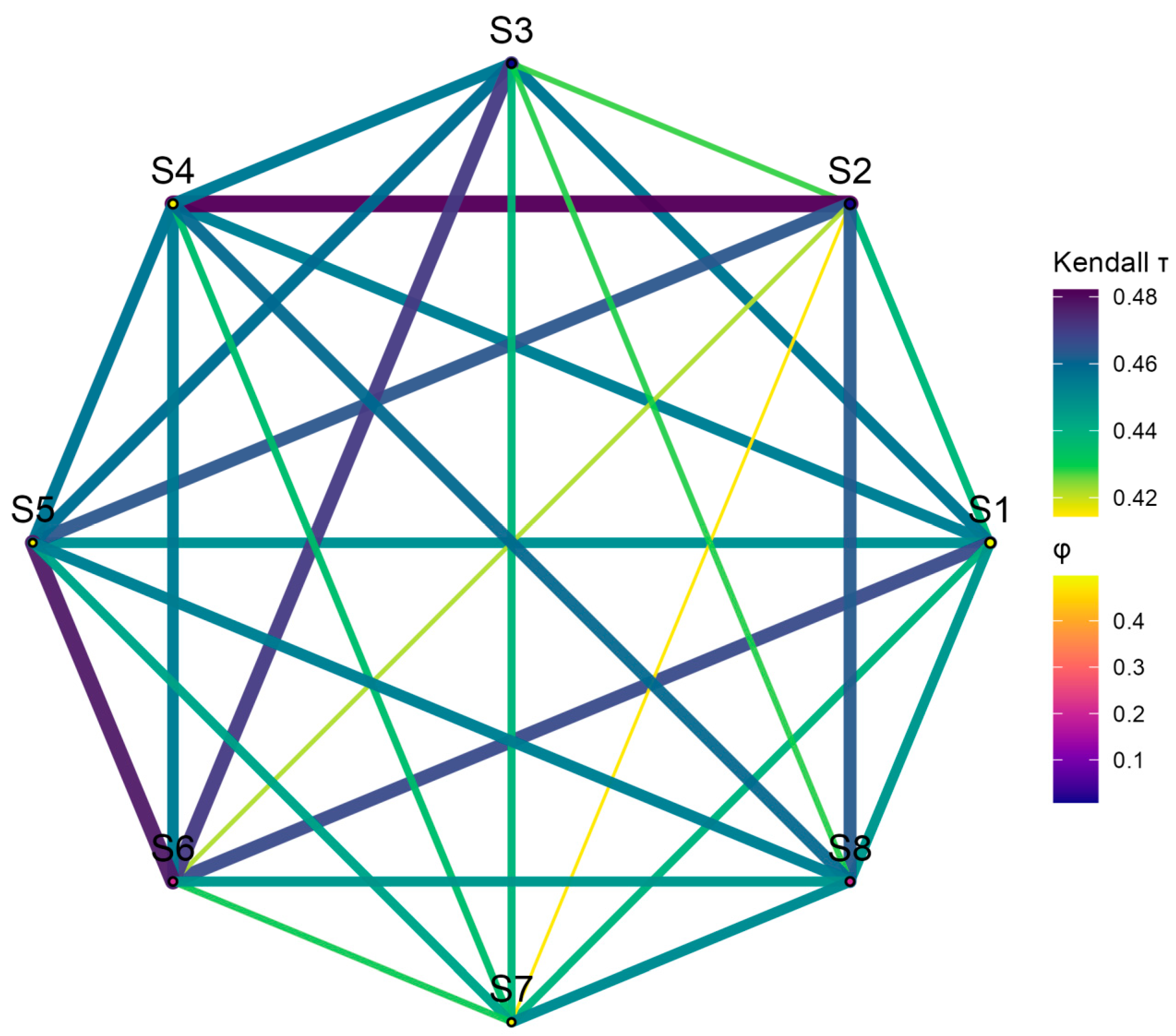
Figure 1. Example schematic design of the synthetic site network used in the simulation experiments for Scenario 5.
Mathematics 13 03762 g001
Figure 2. NSW AMF gauging station locations.
Mathematics 13 03762 g002
Figure 3. Comparison of empirical Type-I error rates (α = 0.05) across eight simulated sites for classical Mann–Kendall (MK), Yue–Wang-corrected MK (YW), and R-CaMK methods. R-CaMK maintains conservative control closest to the nominal 5% level (dashed red line).
Mathematics 13 03762 g003
Figure 4. Detection power across trend slopes (β per year) for MK, Yue–Wang, and R-CaMK methods under independent (solid lines, τ = 0) and moderate (dashed lines, τ = 0.5) spatial dependence scenarios. R-CaMK maintains reliable power while controlling Type-I errors, converging with competing methods at larger slopes.
Mathematics 13 03762 g004
Figure 5. Normal-score pairwise correlations (ρ) among NSW streamflow sites, revealing moderate-to-strong spatial dependence (ρ = 0.01–0.70).
Mathematics 13 03762 g005
Figure 6. R-vine copula structure for NSW streamflow network (Trees 1–3). Each tree sequentially decomposes the seven-dimensional joint distribution into bivariate conditional copulas. (a) Tree 1 links site pairs with the strongest unconditional dependence; (b,c) Trees 2–3 model residual dependence conditional on earlier edges.
Mathematics 13 03762 g006
Figure 7. Spatial dependence Structure: Kendall’s τ from vine copula.
Mathematics 13 03762 g007
Figure 8. Bootstrap diagnostics for ILP-selected sites (210022, 215004, and 219003): null distributions of Mann–Kendall S (left), observed values in red, and normal QQ plots (right) validating the Gaussian approximation of bootstrap replicates.
Mathematics 13 03762 g008
Figure 9. ILP-selected monitoring sites (red).
Mathematics 13 03762 g009
Figure 10. (a) Detection power vs. injected slope for site 219003 (ILP-selected). R-CaMK (blue) outperforms MK and Yue–Wang at moderate slopes, demonstrating superior power under accurate spatial dependence modelling. (b) Detection power vs. injected slope for site 210022 (ILP-selected). Erratic power across methods reflects high bootstrap variance (Var(S) = 67,173) and strong spatial coupling, limiting reliable trend detection at this site. (c) Detection power vs. injected slope for site 215004 (ILP-selected). Yue–Wang shows inflated power at large slopes (β = 0.03), while R-CaMK maintains conservative, reliable inference by correctly accounting for spatial dependence.
Mathematics 13 03762 g010
Table 1. Simulated scenarios grid showing n, T, phi range, Kendall τ range, and slope grid.
Scenarion SitesT (Years)AR(1) φ ValuesKendall’s τ RangeSlope Grid (βj)MC Reps
1880{0, 0.2, 0.5}0.0 (indep.){0}2000
2880{0, 0.2, 0.5}0.1–0.3{0}2000
3880{0, 0.2, 0.5}0.4–0.6{0}2000
4880{0, 0.2, 0.5}0.7–0.9{0}2000
5880{0, 0.2, 0.5}0.0–0.9subset with βj ≠ 0 (e.g., ±0.01 ±0.02 per year)1000
Table 2. Gauging site information (NSW).
Site IDLatitude (°)Longitude (°)T (Years)Catchment
Remarks
215004−35.15150.0389Coastal/Upper Catchment
210011−32.32151.686787Coastal Plain
210017−31.94151.2878Coastal/Small Catchment
210022−32.31151.5178Coastal/Near Headwaters
222004−37149.0977Southern NSW
219003−36.67149.6575Inland River Basin
410061−35.33148.0771Upland River Basin
Table 3. Summary statistics per site (annual maximum flows).
Site IDMean (m3/s)Std Dev (m3/s)SkewnessCV (Std Dev/Mean)
215004183.15151.621.750.83
210011346.32309.91.60.9
21001723.6526.072.261.11
210022199.1142.781.260.72
22200477.6696.053.581.24
219003242.21276.082.81.14
41006153.9957.723.141.07
Table 4. Empirical Type-I error rates across eight simulated sites (nominal α = 0.05).
SiteType1_MKType1_YWType1_RCaMK
10.1330.0910.058
20.1510.0870.049
30.1310.0780.056
40.1360.0840.073
50.120.0780.067
60.140.0870.056
70.1270.1040.062
80.1360.0980.067
Table 5. Sensitivity analysis of Type-I errors and power for R-CaMK under varying complete-case overlap (Tcc), copula family selection, and Gaussian correlation matrix repair. Results are based on representative n = 8, T = 80 simulation scenarios.
ScenarioType-I Error (α = 0.05)Power (β = 0.02)Notes
Vine, Tail Families Enabled
(Tcc ≥ 30)
0.05–0.070.90–0.93Nominal control and robust power
Vine, Gaussian Only0.08–0.120.80–0.85Upward bias under strong/
tail dependence
Gaussian Fallback (Tcc < 30)0.07–0.090.70–0.80More conservative and reduced power
Gaussian Copula w/Matrix Repair0.06–0.100.70–0.80No inflation and conservative under repair
Table 6. (a) NSW streamflow site-level results: trend estimates and AR(1) parameters, Mann–Kendall statistics, bootstrap inference, and detection scores. (b) NSW streamflow site-level results: Mann–Kendall statistics, bootstrap inference, and detection scores.
(a)
SiteIDβOLSβTS ϕ ^ σ η Sobsnobs
210011−0.00820.64150.0455316.5220587
210017−0.2653−0.0208−0.113727.52−9578
2100221.30541.15160.1139136.5244178
215004−0.8552−0.65660.138153.43−36089
219003−1.6253−1.1934−0.0048266.58−36975
222004−0.3678−0.0656−0.090992.28−7877
4100610.0315−0.2916−0.053857.34−28471
(b)
SiteIDVarS_bootp_empp_mk_uncorrectedVIFn_eff_yuewangp_yuewangwj
21001166,221.60.3730.4521870.452320.00003
21001741,429.10.6670.6821780.68190.0013
21002267,173.30.120.0571780.057080.00504
215004100,279.70.3070.2021890.202030.0027
21900341,606.70.080.0911750.091430.00797
22200443,073.90.6930.7321770.731550.00177
41006136,089.20.1330.1591710.158640.00017
Disclaimer/Publisher’s Note: The statements, opinions and data contained in all publications are solely those of the individual author(s) and contributor(s) and not of MDPI and/or the editor(s). MDPI and/or the editor(s) disclaim responsibility for any injury to people or property resulting from any ideas, methods, instructions or products referred to in the content.