Abstract
With the rapid development of modern society and the continuous growth of electricity demand, the stability of power systems has become increasingly critical. In particular, Transient Stability Assessment (TSA) plays a vital role in ensuring the secure and reliable operation of power systems. Existing studies have employed Graph Attention Networks (GAT) to model both the topological structure and vertex attributes of power systems, achieving excellent results under ideal test environments. However, the continuous expansion of power systems and the large-scale integration of renewable energy sources have significantly increased system complexity, posing major challenges to TSA. Traditional methods often struggle to handle various disturbances. To address this issue, we propose a graph attention network framework with multi-branch feature aggregation. This framework constructs multiple GAT branches from different information sources and employs a learnable mask mechanism to enhance diversity among branches. In addition, this framework adopts an uncertainty-aware aggregation strategy to efficiently fuse the information from all branches. Extensive experiments conducted on the IEEE-39 bus and IEEE-118 bus systems demonstrate that our method consistently outperforms existing approaches under different disturbance scenarios, providing more accurate and reliable identification of potential instability risks.
Keywords:
transient stability assessment; Graph Attention Network (GAT); uncertainty-aware aggregation MSC:
68T07
1. Introduction
Power system stability is a core issue for ensuring the secure operation of power systems. With the increasing integration of renewable energy, load fluctuations, and the continuous expansion of grid scale, the dynamic operating characteristics of power systems have become more complex, and the risk of instability has significantly increased [1]. Once a stability issue occurs in the power system, it may trigger large-scale blackouts, resulting in significant economic losses and social impacts. Therefore, accurately and efficiently predicting power system stability has become a critical task in system operation and control. This task carries both significant theoretical importance and practical engineering value.
In recent years, with the development of artificial intelligence technologies, deep learning has gradually become an important tool for predicting power system stability [2]. Compared with traditional methods that rely on numerical simulations and mechanistic modeling, deep learning can more efficiently learn underlying patterns from large amounts of operational data. This approach avoids excessive dependence on complex system parameters and models [3]. Among them, Graph Neural Networks (GNNs) [4,5] have attracted widespread attention because they can effectively capture the complex relationships between the topology of power systems and the features of their vertices [1,6]. Existing studies [7,8] have shown that GNN-based methods achieve promising performance in tasks such as transient stability prediction and fault diagnosis in power systems. These methods offer new approaches for improving both the accuracy and real-time capability of predictions.
However, in real-world power system operations, the collected data is often not completely reliable [9]. On one hand, sensors measuring key quantities such as voltage, current, and power may be affected by electromagnetic interference, communication noise, or environmental factors. This can introduce numerical fluctuations or even abnormal deviations. On the other hand, some monitoring devices may fail due to hardware aging, transmission interruptions, or sudden faults. Such failures lead to missing or incomplete observation data. In this context, the input features relied upon for power system stability prediction may lack accuracy and completeness. Existing methods often assume that input data are reliable and are mainly validated on idealized datasets. They generally do not model robustness under noise or missing data scenarios. Traditional physics-based methods, although theoretically precise, often cannot produce valid results when input information is incomplete. In contrast, data-driven machine learning and deep learning approaches are highly sensitive to input distributions. When disturbances or missing data occur, these methods can easily learn incorrect patterns, resulting in significant performance degradation. Therefore, existing approaches typically exhibit fragility and insufficient robustness in complex interference environments.
To investigate how perturbations affect model prediction performance, we conducted a series of analyses. As shown in Figure 1a, when the model relies on a majority of the grid features, as in deep learning-based methods, it operates in a high-risk state with high probability. This indicates that perturbations in a small subset of features are likely to cause significant performance degradation.
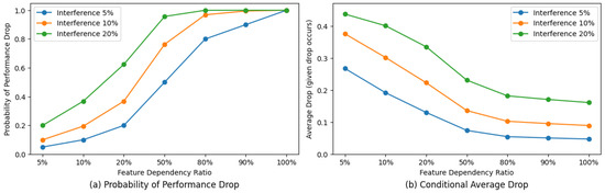
Figure 1.
We first calculate the importance of different features using XGBoost [10]. Then, we select the top 5%, 10%, 20%, 50%, 80%, 90%, and 100% of features, and use them to train an MLP. (a) For the MLPs trained with features at different proportions, we perturb 5%, 10%, and 20% of random features. Through multiple tests, we record the probability of performance degradation. (b) We also compute the average performance degradation across all cases where the MLP shows reduced performance during testing.
In contrast, as shown in Figure 1b, when the model depends only on a few key features, such as in CatBoost [11] or XGBoost [10], it is in a low-probability high-risk state, which means that if these key features are perturbed, the model will experience substantial performance decline. This motivates an evaluation paradigm that can mitigate both the high-probability performance drop caused by minor perturbations and the significant degradation resulting from perturbations in key features.
To address this gap, we propose a multi-branch Graph Attention Network (GAT) for power system transient stability assessment, aiming to enhance model robustness under complex interference. Our approach consists of a diversity information extraction module and an uncertainty-aware information aggregation module. The diversity information extraction module enhances branch diversity through structural differences and feature consistency constraints, where each branch learns a sparse, distinct mask over node/edge features, so every branch relies on only a small, partly disjoint subset of inputs. The uncertainty-aware aggregation module adaptively reduces the weight of branches with unreliable predictions based on uncertainty estimation, thereby producing more robust stability prediction results. Especially, sparse masks reduce the chance that random perturbations simultaneously disrupt many branches, yet if a branch’s own trusted features become unstable, its predictive uncertainty rises; the uncertainty-aware aggregation then down-weights that branch, while retaining contributions from stable branches. We have conducted comprehensive experiments on IEEE-39 and IEEE-118-bus system datasets, which demonstrates that the proposed framework consistently outperforms existing approaches. The results confirm not only the superior robustness and accuracy of the method, but also its potential for practical application in real-world power grid operations.
The main contributions of this work are as follows:
- We propose a multi-branch graph attention network capable of predicting power system stability under noisy conditions. By employing a structural difference constraint algorithm and a feature similarity constraint, the model is encouraged to analyze stability using diverse grid signals.
- We introduce an uncertainty-aware aggregation method. Using an uncertainty estimation mechanism, the approach performs dynamic weighted aggregation when the reliability of branch predictions varies significantly, thereby enhancing the robustness of the final prediction.
- We conduct experiments on the IEEE-39 bus system and IEEE-118-bus system. The results demonstrate that our method outperforms existing approaches under various noise and missing-data scenarios, confirming its effectiveness and practical value.
2. Background and Related Work
2.1. Traditional Methods for Power System Transient Stability Assessment
Early research on power system transient stability assessment primarily relied on physics-based modeling and numerical simulation methods, such as time-domain integration, energy function methods, and Lyapunov approaches. These methods can accurately capture the dynamic behavior of power grids from a physical perspective. However, their high computational complexity makes it difficult to meet real-time requirements. Recent surveys on large-disturbance TSA further categorize mainstream approaches into simulation, direct, data-driven, analytical, and others, and compare their efficiency, accuracy, applicability, and stability-region estimation, providing an updated panorama of TSA research [12]. With the widespread deployment of phasor measurement units (PMUs), researchers have started exploring the integration of grid operation data with machine learning models to improve prediction efficiency. Some studies [13,14] evaluated the transient stability of power systems using Support Vector Machines (SVMs). Other approaches [15,16] employed Artificial Neural Networks (ANNs) to assess the transient stability of power systems. There are also methods [17,18] that analyze the system using decision trees. Gupta D.S. et al. [19] proposed a bi-level optimization approach based on adaptive particle swarm optimization. This method addresses the challenges posed by the integration of renewable energy to transient voltage stability and reliability in power systems. Liu J. et al. [20] extracted the most discriminative signals using low-dimensional projection, clustering, and information-domain feature selection. This approach aims to improve both the efficiency and the accuracy of the assessment.
These data-driven methods offer advantages such as simple model structures, fast training and inference, and relatively good interpretability for small-scale systems. Nevertheless, they typically depend on manually designed features and have limited adaptability to high-dimensional data and complex disturbances, leading to suboptimal performance in large-scale grids and under strong perturbations.
2.2. A Deep Learning-Based Method for Power System Transient Stability Assessment
In recent years, the rise of deep learning techniques has provided new approaches for power system stability prediction. Researchers have employed convolutional neural networks (CNNs) and recurrent neural networks (RNNs/LSTMs) to capture the spatiotemporal dependencies in power grid data. This enables end-to-end modeling without the need for manual feature engineering. Shao et al. [21] proposed an LSTM-SAF model that integrates the self-attention mechanism and focal loss. By combining feature selection with a complete offline–online framework, their approach offers a fast and reliable data-driven solution for transient stability assessment. Similarly, Massaoudi et al. [22] introduced a method based on deep temporal convolutional networks (TCNs) optimized with the Grey Wolf Optimizer (GWO). Their approach provides key state information in the early stage of faults, while improving prediction accuracy and adaptability. Li Y. et al. [23] proposed a transformer-based model for transient stability assessment of power systems. Haoyang B. et al. [24] proposed a two-stage transient stability assessment method based on the Swin Transformer. This approach more effectively extracts temporal information from power system transient data and enhances the interpretability of the model. Li Z. et al. [25] proposed a CNN-based model that effectively improves the accuracy of transient stability assessment in power systems. Kim J. et al. [26] proposed a deep transfer learning method for transient stability assessment of power systems. This method is based on a deep convolutional neural network pretrained on ImageNet. Kesici M. et al. [27] proposed a real-time transient stability prediction framework for power systems that is designed to defend against cyber-attacks. The framework considers both the perspectives of attackers and grid operators to enhance the robustness and security of the prediction under cyber-attack scenarios. Ren C. et al. [28] proposed a secure distributed stability assessment method (SecFedSA) based on federated learning and differential privacy. This method enables decentralized stability prediction and optimization of power systems while ensuring data privacy. Gbadega et al. [29] proposed an OOBO-based energy management framework for RES-rich microgrids that couples K-means clustering and ANN load forecasting to optimally schedule DERs/BESS/diesel generators, achieving lower operating cost and emissions with real-time feasibility.
These methods can automatically learn complex patterns from high-dimensional data. They achieve significantly better accuracy and generalization compared to traditional approaches. However, these methods heavily rely on the distribution of training data and lack modeling of the power system graph structure. As a result, they fail to capture the relationships among different power devices. Therefore, their robustness remains limited in complex and noisy environments.
2.3. A Graph Neural Network-Based Method for Power System Transient Stability Assessment
With the development of Graph Neural Networks (GNNs), an increasing number of studies have begun to model power systems as graph structures. In this approach, electrical devices and monitoring points are represented as vertices, while line parameters and power transmission are represented as edges. This enables GNNs [30] to naturally capture both the topological structure and the feature relationships of the power system. Wang Z. et al. [31] proposed a transient stability assessment model based on steady-state data. This model is built upon a Message Passing Graph Neural Network (MPNN). Huang J. et al. [32] proposed a Graph Convolutional Network (GCN) to explore the topological information of power systems. Zhu L. et al. [33] proposed a spatiotemporal synchronized convolution method for transient stability assessment. Yonghong Luo et al. [34] effectively capture the spatiotemporal features of power systems during transient processes by combining the spatial characteristics of Graph Convolutional Networks (GCNs) with the temporal characteristics of Convolutional Neural Networks (CNNs). Wenting Li et al. [35] proposed a physics-informed Graph Neural Network (PPGN) for real-time fault localization in distribution systems. This method is effective even when observation data are limited. Quang-Ha Ngo et al. [36] combined the physical models of power systems with the learning capability of Graph Neural Networks (GNNs) to achieve more accurate system state estimation. Their approach is particularly effective under conditions of scarce observation data. Liu Z. et al. [37] proposed a GNN-based framework for transient stability assessment of power systems. The framework can provide fast online screening results under varying operating conditions. Zhao H. et al. [38] proposed a transient stability assessment method based on the Spatio-Temporal Broad Learning System (STBLS). By integrating the Broad Learning System (BLS), Graph Convolutional Network (GCN), and Temporal Convolutional Network (TCN) [39], the method achieves fast and accurate evaluation of the transient stability of power systems.
The advantage of this type of method lies in its ability to fully exploit power grid topology, thereby enhancing modeling capability and prediction performance. However, most existing studies assume that the input data is reliable. They lack systematic modeling for measurement noise, missing features, and uncertainty. In addition, their information aggregation strategies are often fixed, making it difficult to adjust dynamically when branch predictions diverge. As a result, robustness under noisy or disturbed environments remains insufficient.
3. Materials and Methods
Overview
Our framework is illustrated in Figure 2. To fully exploit the topology of the power grid, we model the grid as a graph that contains both vertex features and edge features. This graph is then used as the input to the graph attention network. The formal definition is as follows:
- Vertex: Each vertex represents either an electrical device or a voltage monitoring point. The vertex feature vector contains local features that can be directly measured or derived at this point. Examples include voltage magnitude, voltage phase angle, and the active/reactive power outputs of generators directly connected to the vertex.
- Edge: An edge represents the transmission line that directly connects two vertices and . The edge feature is defined by the operational parameters of the line, such as active power, reactive power, admittance, or power flow direction. These features describe the energy transmission between vertices and the strength of their coupling.
Accordingly, the power grid can be formalized as a weighted graph with edge features:
where X denotes all vertex features, and E denotes all edge features. The stability analysis task of a power grid under interference can be formulated as training a model . In this formulation, and , where noise represents a noise function that introduces disturbances into the features X and E. The output label indicates whether the power grid remains stable.

Figure 2.
Overview of the proposed model. It has two components: (1) a multi-branch extractor, where each branch applies graph attention and receives different inputs via learnable edge and node masks (, ) optimized to encourage diversity; (2) an uncertainty-aware aggregator that fuses branch outputs using predicted entropy and a mask-reliability score.

4. Method
4.1. Graph Attention Network
In power grid stability prediction, the electrical coupling relationships between vertices are highly complex. Traditional graph convolutional networks (GCNs) [40], which rely solely on neighbor aggregation, cannot effectively distinguish the importance of different neighbors to the target vertex. Graph Attention Networks (GATs) [41] introduce an attention mechanism that adaptively learns the weights of neighbors during aggregation. This allows GATs to better capture the relationships between the grid topology and operational characteristics.
To further enhance the modeling capability, we incorporate edge features into GAT. In this way, the attention weights depend not only on vertex features but also on the operational state of transmission lines. Specifically, let the feature vector of vertex i be , and that of its neighbor vertex j be . Meanwhile, the edge feature is denoted as . First, we obtain the projected features through a linear transformation:
where and are learnable parameters, which are used for feature extraction of vertices and edges, respectively. Both are mapped into a feature space of the same dimension. Subsequently, the attention coefficient is computed using the following formula:
where a denotes the attention vector, and ‖ represents the concatenation operation. This mechanism ensures that different neighbors and their corresponding edge features receive differentiated weights during information propagation. Finally, the representation of vertex i can be obtained through weighted aggregation:
where denotes a nonlinear activation function. In this way, the GAT can simultaneously capture the topological dependencies of the power grid (determined by adjacency relationships), the local measurement features (vertex features), and the operational states of the lines (edge features). Therefore, the edge-feature-based GAT not only learns the complex dependencies in the power grid from a data-driven perspective, but also aligns with the physical intuition of power system operations.
4.2. Multi-Branch Feature Extraction Module
Although a single Graph Attention Network (GAT) can effectively model the topology and measurement data of power grids, its prediction performance often relies heavily on global features in complex interference environments. This reliance makes the model vulnerable, since small perturbations may disrupt the underlying data assumptions.
To improve robustness under such conditions, we introduce a multi-branch architecture based on feature-dependent GAT. Specifically, in each branch, the input feature matrix X is modulated by a learnable mask matrix :
where denotes the modulated features, ⊙ represents element-wise multiplication, and controls the subset of vertex features accessible to this branch. Similarly, the input edge feature matrix E is modulated by a structural mask matrix , resulting in adjusted edge features:
To encourage different branches to rely on distinct sources of information, we design a structural difference constraint:
where denotes the mask of the i-th branch. Specifically, we compute a corresponding for the edge feature mask and the vertex feature mask, respectively. At the same time, to prevent most branches from being negatively affected when only a few signals are disturbed, we introduce a mask sparsity constraint loss:
On this basis, the mask loss of our proposed multi-branch information extraction module can be formulated as:
where denotes the classification loss of the model, which is implemented using cross-entropy loss. The parameters and are the weighting coefficients of the loss.
Since the stability of a power grid is an inherent global property, different feature subsets only represent the same system state from different perspectives. Therefore, although each branch relies on a different feature subset, their predictions of system stability should remain consistent or close to each other. To achieve this, we introduce a branch prediction consistency constraint:
where denotes the i-th feature extractor. On this basis, the model loss of our proposed multi-branch information extraction module can be formulated as:
where is a weight parameter. Finally, we can control the signal input of different branches through the dynamically updated feature masks and . Then, we extract high-dimensional information in the same feature space using GAT. This process enhances the robustness of the model.
4.3. Uncertainty-Aware Aggregation
In the multi-branch architecture, each branch performs information selection through dual masks on vertex and edge features. A graph attention network with edge features is then used to extract feature representations related to local stability. However, the prediction capability of different branches may vary. On the one hand, due to different mask selections, some branches may rely on insufficient or redundant key information, which leads to biased results. On the other hand, in complex interference environments, the extracted features of certain branches may be distorted by noise. If the outputs of all branches are simply averaged or fused with fixed weights, unreliable branches may introduce noise, thereby degrading overall prediction performance. To address this issue, we propose an uncertainty-aware feature aggregation mechanism. This mechanism adaptively adjusts the weights at the branch level, thus improving the robustness of the overall model.
For the feature produced by each branch, we first mask out the features from the other branches. Then, we apply Monte Carlo dropout to perform multiple forward passes, obtaining a set of predictive samples :
where denotes the classifier. Based on this, the uncertainty of each branch can be measured by the prediction entropy:
where a higher level of uncertainty indicates that the predictions of a branch are less stable under the current input. In addition, the masks in the multi-branch architecture naturally provide dependency information for each branch. Let the vertex mask be denoted as and the edge mask as . Their coverage can then be defined as:
A larger coverage indicates that a branch relies on more features, which may introduce additional noise interference. Conversely, an excessively small coverage may lead to insufficient information. In this paper, we define the mask reliability factor as follows:
where is a hyperparameter that balances the sparsity and reliability of the mask. Based on this, we can compute the reliability score for each branch:
Furthermore, by applying normalization, we compute the aggregation weight of each branch to obtain the aggregated features. The detailed procedure is presented in Algorithm 1.
| Algorithm 1 Uncertainty-Aware Aggregation Algorithm |
| Input: The feature set is denoted as , the vertex mask set as , and the edge mask set as . Output: Fused feature |
| 1: Initialize the aggregated feature as a zero matrix. |
| 2: for i in do |
| 3: The predicted probability is calculated according to Equation (11). |
| 4: The predictive entropy of branch i is calculated according to Equation (12). |
| 5: According to Equations (13) and (14), the point coverage and the edge coverage are calculated. |
| 6: The mask reliability factor is computed according to Equation (15). |
| 7: |
| 8: end for |
| 9: return |
5. Experiment
5.1. Dataset
The IEEE 39-bus system consists of 39 buses, 10 generators, and 46 branches. The IEEE 118-bus system consists of 118 buses, 54 generators, 91 loads, and 186 branches. Time-domain simulations of the IEEE 39-bus and IEEE 118-bus systems are conducted using the Power System Analysis Toolbox (PSAT, Version 2.1.11) [42] and MATPOWER (Version 7.1) [43] in MATLAB R2023b.
5.2. Implementation Details
Our experiments were conducted on an NVIDIA GeForce RTX 4090 GPU (NVIDIA Corporation, Santa Clara, CA, USA), with CUDA 12.4, PyTorch 2.3.0, and PyTorch Geometric 2.5.3. The learning rate was fixed at , the batch size was set to 16, and the training was run for 200 epochs. We selected hyperparameters by grid search on the validation split and then fixed them for testing. We use B = 8 GAT branches to extract features in power grid topology. For losses, the mask-loss weights are set to , , and the alignment-loss weight is . For uncertainty-aware aggregation, we use for entropy weight and for coverage penalty. These settings are used for all reported results.
To comprehensively evaluate the robustness of the proposed method under different disturbance environments, we consider several typical sources of uncertainty in power system operations. Specifically, we define the following disturbance types:
- Feature Missing: Some measurements may be unavailable due to equipment aging or failure. We simulate this disturbance by removing a portion of the feature signals.
- Measurement Error: Measurement devices may be affected by external perturbations, resulting in errors. We simulate this disturbance by adding zero-mean Gaussian noise to the feature signals.
- Abnormal Fluctuations: Sudden fluctuations may occur due to external factors such as weather conditions. We simulate this disturbance by replacing feature values with extreme high or low values.
We further combine the above disturbances randomly to better approximate real-world scenarios. More specifically, we randomly apply these three types of disturbances to of the original features. In all scenarios, we evaluate the performance using the test set, record the accuracy and F1-score, and compare the results against baseline methods.
5.3. Performance Analysis of Models Under Perturbations
To investigate the performance of our proposed framework under different levels of perturbation, we designed scenarios with 0%, 5%, 10%, 20%, and 50% perturbation. We then evaluated the framework using various models. From Table 1 and Table 2, it can be seen that under zero perturbation (0%), our method achieves the highest ACC and F1 scores among all compared models. Specifically, for the 39-bus system, our method reaches 98.69% ACC and 98.70% F1, and for the 118-bus system, it reaches 87.83% ACC and 88.26% F1. The improvement under the no-perturbation condition indicates that our method effectively captures the latent features of the power system. This is attributed to the design of the multi-branch feature extraction module, which encourages the model to learn richer mappings from features to stability assessment. Meanwhile, the uncertainty-aware module effectively aggregates the results of multiple mappings, thereby enhancing the overall performance of the model.

Table 1.
The results of various methods tested on the IEEE 39-bus system are shown. ACC denotes accuracy, and F1 denotes the F1 score. The best results are highlighted in bold.
Table 2.
The results of various methods tested on the IEEE 118-bus system are shown. ACC denotes accuracy, and F1 denotes the F1 score. The best results are highlighted in bold.
When perturbations are introduced (5%, 10%, 20% and 50%), all baseline models (MLP, CNN, GCN, GAT) show significant performance degradation. For instance, in the 39-bus system, MLP’s ACC drops from 95.44% to 53.36%, while CNN drops from 96.25% to 59.63% at 50% perturbation. In contrast, our method maintains a high performance level even under severe perturbations, with ACC/F1 scores of 87.46%/87.20% for 39-bus and 74.63%/73.71% for 118-bus at 50% perturbation. This demonstrates that our method is highly robust to input perturbations, significantly reducing the negative impact of disturbances.
To intuitively demonstrate the performance changes of various methods under different levels of perturbations, we plotted a bar chart. As shown in Figure 3, the performance of the baseline methods drops sharply as the perturbation increases. In contrast, our method is able to maintain a relatively high performance. This indicates that the proposed approach can effectively handle perturbations of varying intensities.
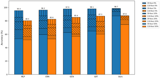
Figure 3.
Performance of various models under different levels of perturbation.
5.4. Ablation Study
5.5. Effectiveness Analysis
To evaluate the contributions of the two key modules in our proposed framework, we conducted an ablation study on the Multi-branch Feature Extraction and Uncertainty-Aware Aggregation modules. Table 3 presents the results in terms of ACC and F1 under different perturbation levels.
Table 3.
Ablation study of two modules on ACC and F1 (%). Variant 0: This variant is composed of GAT and does not include the Multi-branch Feature Extraction Module or the Uncertainty-Aware Aggregation. Variant 1: This variant only includes the Multi-branch Feature Extraction Module. The features from multiple branches are averaged to obtain the aggregated feature . Variant 2: This variant only uses the Uncertainty-Aware Aggregation module. We employ multiple GATs without any additional processing as independent branches. Variant 3: This variant simultaneously incorporates the Multi-branch Feature Extraction Module and the Uncertainty-Aware Aggregation. And the best results are highlighted in bold.
Comparing Variant 1 with Variant 0, we observe a significant improvement in both ACC and F1 across all perturbation levels. This indicates that the Multi-branch Feature Extraction module effectively enhances the model’s robustness. It is noteworthy that under a 5% perturbation, Variant 1 only improves the ACC on the IEEE 39-bus system by 7.28%. However, under a 50% perturbation, the ACC increases by 21.87%. A similar trend is also observed on the IEEE 118-bus system. This indicates that Variant 1 enhances the model’s robustness against disturbances. This behavior aligns with expectations, as the multi-branch architecture provides diverse feature sources. Even when some branches are affected by perturbations, the aggregated feature, obtained through averaging, remains stable and reliable, thereby improving overall anti-interference capability.
Variant 2 contains only the uncertainty-aware aggregation module. Its performance is also improved compared to Variant 0. However, these improvements are relatively minor. On the IEEE 39-bus system, Variant2 achieves only a performance gain under a perturbation. Since Variant 2 aggregates multiple GAT structures without additional feature diversity, the main source of enhancement stems from the increased model capacity rather than a substantial robustness gain.
Variant 3 integrates multi-branch feature extraction and an uncertainty-aware aggregation module. It achieves the best performance across all perturbation levels on both datasets. The combination of the Multi-branch Feature Extraction and Uncertainty-Aware Aggregation modules leverages diverse feature extraction while adaptively weighting the contributions of each branch according to uncertainty. This synergistic effect allows Variant 3 to outperform both Variant 1 and Variant 2, demonstrating that both modules are indispensable for maximizing the model’s predictive accuracy and robustness under perturbations.
5.6. Effectiveness Analysis of the Multi-Branch Information Extraction Module
To investigate the impact of each loss term in the multi-branch information extraction module on model performance, we conducted an ablation study. Table 4 lists the accuracy (ACC) and F1 scores of the model on the 39-bus and 118-bus datasets under different combinations of losses.
Table 4.
w/o denotes that no additional operation is performed. indicates that only is used to update the mask matrix, where the model is optimized solely based on the cross-entropy loss. means that only is used to update the model, while the mask is randomly generated and kept fixed. Ours (i.e., ), represents the complete multi-branch information extraction module. And the best results are highlighted in bold.
Compared with the baseline model without any loss (w/o), introducing only the structural discrepancy loss increased the average ACC on the 39-bus dataset from 82.75% to 90.97%, and the F1 score from 82.00% to 90.43%. On the 118-bus dataset, the average ACC improved from 77.37% to 80.12%, and the F1 score from 77.03% to 79.77%. As the perturbation intensity increased, the performance gains also increased. This indicates that the structural discrepancy loss significantly enhances the model’s robustness to disturbances. The improvement occurs because the optimization objective of is to increase the diversity of input feature structures across different branches, thereby improving the model’s robustness against various perturbations.
Further, adding the feature consistency loss led to an average ACC of 92.98% and F1 of 92.44% on the 39-bus dataset. On the 118-bus dataset, the average ACC and F1 increased to 81.49% and 80.84%, respectively. The performance improvement became more stable and continuous. This is because the objective of is to enhance the consistency of output features across branches, which helps extract valuable information more effectively during feature aggregation and thus improves overall performance.
Finally, the complete multi-branch information extraction module () further improves performance compared with and . On the 39-bus dataset, the average ACC and F1 reached 94.92% and 94.70%, respectively. On the 118-bus dataset, they reached 83.18% and 82.93%, respectively. This indicates that the combination of the two components further optimizes the feature representation, enabling the model to achieve optimal robustness and overall performance. We then manually analyze one branch on the IEEE 39-bus system, and its mask concentrates on generator-centric cues—bus voltage and nearby generators’ active/reactive power—while largely suppressing load variables. These signals are directly tied to transient stability: voltage depression and abrupt changes in generator P/Q often precede angle separation, diminished synchronizing torque, and post-fault divergence. The mask is denser on generator buses and along adjacent corridors, yielding features that are highly diagnostic of stable or unstable outcomes after large disturbances, which is physically plausible and aligned with TSA practice.
5.7. Effectiveness Analysis of the Uncertainty-Aware Aggregation Module
To investigate the impact of prediction entropy and mask reliability coefficients on model performance in the Uncertainty-Aware Aggregation (UAA) module, we conducted an ablation study. Table 5 presents the accuracy (ACC) and F1 scores of the model on the 39-bus and 118-bus datasets under different aggregation strategies.
Table 5.
Variant 0: This variant does not employ our proposed uncertainty-aware aggregation algorithm. Instead, it aggregates features using a simple averaging method. Variant 1: This variant uses only the predictive entropy as the aggregation coefficient, defined as . Variant 2: This variant employs the full uncertainty-aware aggregation algorithm. And the best results are highlighted in bold.
From Variant 0 to Variant 1, we observe that using prediction entropy alone as the aggregation coefficient increases the average ACC on the 39-bus dataset from 91.69% to 93.36%, and the F1 score from 90.94% to 92.40%. On the 118-bus dataset, the average ACC rises from 80.21% to 82.72%, and the F1 score from 79.47% to 83.35%. This indicates that leveraging only the prediction entropy can provide a certain degree of weighted feature aggregation, thereby improving overall performance.
Furthermore, when employing the complete uncertainty-aware aggregation algorithm (Variant 2), the model achieves an average ACC of 94.92% and F1 of 94.70% on the 39-bus dataset, and an ACC of 83.18% and F1 of 82.93% on the 118-bus dataset. Compared with Variant 1, the performance shows a significant improvement, especially under strong perturbations. Since the mask reliability coefficient is directly related to the signal input of each branch, it is more sensitive to feature perturbations. This allows the model to adjust the weight of each branch.
6. Discussion and Future Work
This work targets moderate-size benchmarks (IEEE 39- and 118-bus), on which the proposed multi-branch GAT with MC dropout trains and infers efficiently on commodity hardware. Even in the worst-case scenario of a fully connected graph topology, the overall computational cost scales as ), where B is the number of GAT branches and d is the node feature dimension. Given the modest node counts (39 or 118), this complexity remains manageable. We acknowledge that scaling to much larger grids (e.g., thousands of buses) can increase both latency and memory.
Additionally, our future research will focus on several directions. First, we will extend robustness to large, dynamically evolving grids naturally points to zonal partitioning, cluster-wise GNNs, etc., to sustain real-time performance. Second, while our current UQ uses MC dropout and already improves performance and robustness under noisy or missing inputs, it remains a convenient but low-fidelity proxy, motivating higher-fidelity UQ (e.g., deep ensembles, Bayesian/variational GNN layers) with calibration checks. Third, incorporating physical priors and domain knowledge can enhance generalization and interpretability. Finally, we will design a lightweight path toward TSA/EMS integration—streaming PMU/SCADA adapters, single-pass online inference under a latency budget, and a simple gRPC/REST scoring service exposing confidence—that facilitates practical validation in dispatch platforms.
7. Conclusions
This paper investigates the challenge of robustness in power system transient stability assessment under complex interference environments, where factors such as input noise and missing features can severely degrade prediction performance. To address this problem, we propose a prediction framework based on a multi-branch Graph Attention Network (GAT), which integrates structural modeling, multi-branch feature extraction, and uncertainty-aware fusion to achieve accurate and reliable predictions.
Specifically, the proposed method first establishes a graph-based representation of the power grid, effectively embedding both topological structures and operational features. To capture intricate correlations among grid vertices, an edge-feature-enhanced GAT is introduced, which strengthens the interaction between vertex states and edge attributes. Building on this foundation, we design a multi-branch feature extraction mechanism equipped with dual masks and branch constraints. This mechanism promotes feature sparsity and diversity, thereby mitigating the adverse effects of perturbations on individual features. In addition, an uncertainty-aware aggregation module is developed to dynamically fuse the predictions from different branches. By incorporating both prediction uncertainty and mask reliability into the weighting process, the module adaptively balances contributions from diverse branches, enhancing robustness while improving interpretability of the final results. Comprehensive experiments conducted on multiple interference scenarios—including feature loss, noise perturbations, and their combined effects—demonstrate that the proposed framework consistently outperforms existing approaches. The results confirm not only the superior robustness and accuracy of the method, but also its potential for practical application in real-world power grid operations.
Author Contributions
Methodology: K.W.; Writing—Original Draft: S.F., K.J.;Writing—Review & Editing: H.X., J.H. All authors have read and agreed to the published version of the manuscript.
Funding
This research was funded by the Science and Technology Foundation of State Grid Corporation of China (Grant/Award Number: 5100-202355764A-3-5-YS), The Science and Technology Innovation Program of Hunan Province (2025RC3012), Natural Science Foundation of Hunan Province (2025JJ60229).
Data Availability Statement
The raw data supporting the conclusions of this article will be made available by the authors on request.
Conflicts of Interest
The authors declare no conflicts of interest.
References
- Nauck, C.; Lindner, M.; Schürholt, K.; Zhang, H.; Schultz, P.; Kurths, J.; Isenhardt, I.; Hellmann, F. Predicting basin stability of power grids using graph neural networks. New J. Phys. 2022, 24, 043041. [Google Scholar] [CrossRef]
- Wang, S.; Xiang, X.; Zhang, J.; Liang, Z.; Li, S.; Zhong, P.; Zeng, J.; Wang, C. A multi-task spatiotemporal graph neural network for transient stability and state prediction in power systems. Energies 2025, 18, 1531. [Google Scholar] [CrossRef]
- Shahzad, U. Artificial neural network for transient stability assessment: A review. In Proceedings of the 2024 29th International Conference on Automation and Computing (ICAC), Sunderland, UK, 28–30 August 2024; pp. 1–7. [Google Scholar]
- Scarselli, F.; Tsoi, A.C.; Gori, M.; Hagenbuchner, M. Graphical-based learning environments for pattern recognition. In Joint IAPR International Workshops on Statistical Techniques in Pattern Recognition (SPR) and Structural and Syntactic Pattern Recognition (SSPR); Springer: Berlin/Heidelberg, Germany, 2004; pp. 42–56. [Google Scholar]
- Scarselli, F.; Gori, M.; Tsoi, A.C.; Hagenbuchner, M.; Monfardini, G. The graph neural network model. IEEE Trans. Neural Netw. 2008, 20, 61–80. [Google Scholar] [CrossRef]
- Zhang, Y.; Karve, P.M.; Mahadevan, S. Graph neural networks for power grid operational risk assessment under evolving grid topology. arXiv 2024, arXiv:2405.07343. [Google Scholar] [CrossRef]
- Suri, D.; Mangal, M. PowerGNN: A Topology-Aware Graph Neural Network for Electricity Grids. arXiv 2025, arXiv:2503.22721. [Google Scholar]
- Deng, C.; Dai, L.; Chao, W.; Huang, J.; Wang, J.; Lin, L.; Qin, W.; Lai, S.; Chen, X. An Advanced Spatio-Temporal Graph Neural Network Framework for the Concurrent Prediction of Transient and Voltage Stability. Energies 2025, 18, 672. [Google Scholar] [CrossRef]
- Jafarzadeh, S.; Genc, V.I. Real-time transient stability prediction of power systems based on the energy of signals obtained from PMUs. Electr. Power Syst. Res. 2021, 192, 107005. [Google Scholar] [CrossRef]
- Chen, T.; Guestrin, C. Xgboost: A scalable tree boosting system. In Proceedings of the 22nd ACM SIGKDD International Conference on Knowledge Discovery and Data Mining, San Francisco, CA, USA, 13–17 August 2016; pp. 785–794. [Google Scholar]
- Prokhorenkova, L.; Gusev, G.; Vorobev, A.; Dorogush, A.V.; Gulin, A. CatBoost: Unbiased boosting with categorical features. Adv. Neural Inf. Process. Syst. 2018, 31, 6639–6649. [Google Scholar]
- Wu, H.; Li, J.; Yang, H. Research methods for transient stability analysis of power systems under large disturbances. Energies 2024, 17, 4330. [Google Scholar] [CrossRef]
- Moulin, L.; Da Silva, A.A.; El-Sharkawi, M.; Marks, R.J. Support vector machines for transient stability analysis of large-scale power systems. IEEE Trans. Power Syst. 2004, 19, 818–825. [Google Scholar] [CrossRef]
- Gomez, F.R.; Rajapakse, A.D.; Annakkage, U.D.; Fernando, I.T. Support vector machine-based algorithm for post-fault transient stability status prediction using synchronized measurements. IEEE Trans. Power Syst. 2010, 26, 1474–1483. [Google Scholar] [CrossRef]
- Amjady, N.; Majedi, S.F. Transient stability prediction by a hybrid intelligent system. IEEE Trans. Power Syst. 2007, 22, 1275–1283. [Google Scholar] [CrossRef]
- Hashiesh, F.; Mostafa, H.E.; Khatib, A.R.; Helal, I.; Mansour, M.M. An intelligent wide area synchrophasor based system for predicting and mitigating transient instabilities. IEEE Trans. Smart Grid 2012, 3, 645–652. [Google Scholar] [CrossRef]
- He, M.; Zhang, J.; Vittal, V. Robust online dynamic security assessment using adaptive ensemble decision-tree learning. IEEE Trans. Power Syst. 2013, 28, 4089–4098. [Google Scholar] [CrossRef]
- Rahmatian, M.; Chen, Y.C.; Palizban, A.; Moshref, A.; Dunford, W.G. Transient stability assessment via decision trees and multivariate adaptive regression splines. Electr. Power Syst. Res. 2017, 142, 320–328. [Google Scholar] [CrossRef]
- Gupta, D.S.; Kolikipogu, R.; Pittala, V.S.; Sivakumar, S.; Pittala, R.B.; Al Ansari, D.M.S. Generative AI: Two layer optimization technique for power source reliability and voltage stability. J. Theor. Appl. Inf. Technol. 2024, 102, 5894–5903. [Google Scholar]
- Liu, J.; Liu, J.; Liu, X.; Liu, X.; Zhao, Y. Discriminative signal recognition for transient stability assessment via discrete mutual information approximation and Eigen decomposition of Laplacian matrix. IEEE Trans. Ind. Inform. 2023, 20, 5805–5817. [Google Scholar] [CrossRef]
- Shao, Z.; Wang, Q.; Cao, Y.; Cai, D.; You, Y.; Lu, R. A novel data-driven LSTM-SAF model for power systems transient stability assessment. IEEE Trans. Ind. Inform. 2024, 20, 9083–9097. [Google Scholar] [CrossRef]
- Massaoudi, M.; Zamzam, T.; Eddin, M.E.; Ghrayeb, A.; Abu-Rub, H.; Refaat, S.S. Fast transient stability assessment of power systems using optimized temporal convolutional networks. IEEE Open J. Ind. Appl. 2024, 5, 267–282. [Google Scholar] [CrossRef]
- Li, Y.; Cao, J.; Xu, Y.; Zhu, L.; Dong, Z.Y. Deep learning based on Transformer architecture for power system short-term voltage stability assessment with class imbalance. Renew. Sustain. Energy Rev. 2024, 189, 113913. [Google Scholar] [CrossRef]
- Haoyang, B.; Jun, A.; Yibo, Z. Transient Stability Assessment of Power Systems Based on Shift Window Self-Attention Swin Transformer. In Proceedings of the Electrical Artificial Intelligence Conference, Nanjing, China, 6–8 December 2024; pp. 77–88. [Google Scholar]
- Li, Z.; Yan, J.; Liu, Y.; Liu, W.; Li, L.; Qu, H. Power system transient voltage vulnerability assessment based on knowledge visualization of CNN. Int. J. Electr. Power Energy Syst. 2024, 155, 109576. [Google Scholar] [CrossRef]
- Kim, J.; Lee, H.; Kim, S.; Chung, S.H.; Park, J.H. Transient stability assessment using deep transfer learning. IEEE Access 2023, 11, 116622–116637. [Google Scholar] [CrossRef]
- Kesici, M.; Mohammadpourfard, M.; Aygul, K.; Genc, I. Deep learning-based framework for real-time transient stability prediction under stealthy data integrity attacks. Electr. Power Syst. Res. 2023, 221, 109424. [Google Scholar] [CrossRef]
- Ren, C.; Yu, H.; Yan, R.; Li, Q.; Xu, Y.; Niyato, D.; Dong, Z.Y. SecFedSA: A secure differential-privacy-based federated learning approach for smart cyber–physical grid stability assessment. IEEE Internet Things J. 2023, 11, 5578–5588. [Google Scholar] [CrossRef]
- Gbadega, P.A.; Sun, Y.; Balogun, O.A. Optimized energy management in Grid-Connected microgrids leveraging K-means clustering algorithm and Artificial Neural network models. Energy Convers. Manag. 2025, 336, 119868. [Google Scholar] [CrossRef]
- Gori, M.; Monfardini, G.; Scarselli, F. A new model for learning in graph domains. In Proceedings of the 2005 IEEE International Joint Conference on Neural Networks, Montreal, QC, Canada, 31 July–4 August 2005; Volume 2, pp. 729–734. [Google Scholar]
- Wang, Z.; Zhou, Y.; Guo, Q.; Sun, H. Transient stability assessment of power system considering topological change: A message passing neural network-based approach. Proc. CSEE 2021, 41, 2341–2350. [Google Scholar]
- Huang, J.; Guan, L.; Su, Y.; Yao, H.; Guo, M.; Zhong, Z. Recurrent graph convolutional network-based multi-task transient stability assessment framework in power system. IEEE Access 2020, 8, 93283–93296. [Google Scholar] [CrossRef]
- Zhu, L.; Hill, D.J.; Lu, C. Intelligent short-term voltage stability assessment via spatial attention rectified RNN learning. IEEE Trans. Ind. Inform. 2020, 17, 7005–7016. [Google Scholar] [CrossRef]
- Luo, Y.; Lu, C.; Zhu, L.; Song, J. Data-driven short-term voltage stability assessment based on spatial-temporal graph convolutional network. Int. J. Electr. Power Energy Syst. 2021, 130, 106753. [Google Scholar] [CrossRef]
- Li, W.; Deka, D. PPGN: Physics-preserved graph networks for real-time fault location in distribution systems with limited observation and labels. arXiv 2021, arXiv:2107.02275. [Google Scholar]
- Ngo, Q.H.; Nguyen, B.L.; Vu, T.V.; Zhang, J.; Ngo, T. Physics-informed graphical neural network for power system state estimation. Appl. Energy 2024, 358, 122602. [Google Scholar] [CrossRef]
- Liu, Z.; Ding, Z.; Huang, X.; Zhang, P. An online power system transient stability assessment method based on graph neural network and central moment discrepancy. Front. Energy Res. 2023, 11, 1082534. [Google Scholar] [CrossRef]
- Zhao, H.; Ni, R. Power System Transient Stability Assessment Based on Spatio-Temporal Broad Learning System. IEEE Trans. Autom. Sci. Eng. 2025, 22, 10343–10353. [Google Scholar] [CrossRef]
- Bai, S.; Kolter, J.Z.; Koltun, V. An empirical evaluation of generic convolutional and recurrent networks for sequence modeling. arXiv 2018, arXiv:1803.01271. [Google Scholar] [CrossRef]
- Kipf, T. Semi-supervised classification with graph convolutional networks. arXiv 2016, arXiv:1609.02907. [Google Scholar]
- Veličković, P.; Cucurull, G.; Casanova, A.; Romero, A.; Lio, P.; Bengio, Y. Graph attention networks. arXiv 2017, arXiv:1710.10903. [Google Scholar]
- Milano, F. An open source power system analysis toolbox. IEEE Trans. Power Syst. 2005, 20, 1199–1206. [Google Scholar] [CrossRef]
- Zimmerman, R.D.; Murillo-Sánchez, C.E.; Gan, D. MATPOWER: A MATLAB power system simulation package. Manual Power Syst. Eng. Res. Center Ithaca NY 1997, 1, 10–17. [Google Scholar]


Disclaimer/Publisher’s Note: The statements, opinions and data contained in all publications are solely those of the individual author(s) and contributor(s) and not of MDPI and/or the editor(s). MDPI and/or the editor(s) disclaim responsibility for any injury to people or property resulting from any ideas, methods, instructions or products referred to in the content. |
© 2025 by the authors. Licensee MDPI, Basel, Switzerland. This article is an open access article distributed under the terms and conditions of the Creative Commons Attribution (CC BY) license (https://creativecommons.org/licenses/by/4.0/).