Decomposition-Aware Framework for Probabilistic and Flexible Time Series Forecasting in Aerospace Electronic Systems

Abstract

Degradation prediction for aerospace electronic systems plays a crucial role in maintenance work. This paper proposes a concise and efficient framework for multivariate time series forecasting that is capable of handling diverse sequence representations through a Channel-Independent (CI) strategy. This framework integrates a decomposition-aware layer to effectively separate and fuse global trends and local variations and a temporal attention module to capture temporal dependencies dynamically. This design enables the model to process multiple distinct sequences independently while maintaining the flexibility to learn shared patterns across channels. Additionally, the framework incorporates probabilistic distribution forecasting using likelihood functions, addressing the dynamic variations and uncertainty in time series data. The experimental results on multiple real-world datasets validate the framework’s effectiveness, demonstrating its robustness and adaptability in handling diverse sequences across various application scenarios.

1. Introduction

Modern aerospace equipment is advancing towards a higher performance and intelligence. Due to the harsher environmental conditions in space, aerospace electronic systems require higher reliability. These systems are subject to long-term exposure to various stresses, such as electrical, thermal, and humidity stresses, leading to degradation in their critical components. When this degradation exceeds the design’s fault tolerance, the functionality of electronic products will become abnormal, affecting the spacecraft’s normal operation. Therefore, electronic systems need to collect key characteristic data to predict the future health status of electronic devices by analyzing current and historical data. This predictive degradation monitoring enables condition-based maintenance, effectively reducing maintenance costs [1,2].

In recent years, the rapid advancement of sensor technology and network communications has made it possible to generate and accumulate time series data from electronic systems. Compared with traditional forecasting models, time series models emphasize uncovering the inherent patterns within the temporal dimension. Extracting these patterns from historical time series data facilitates predicting future trends and developments.

For electronic devices, multiple key indicators often represent the health status of the equipment comprehensively. For instance, in the case of flight control computers, the degradation state is primarily evaluated using parameters such as crystal oscillators, analogue-to-digital and digital-to-analogue signals (AD/DA), optocouplers, and total power output. Consequently, this generally involves multivariate time series forecasting, where the future trends in multiple variables are predicted based on historical data. To effectively forecast these trends across multiple key indicators, it is particularly important to develop models capable of simultaneously predicting multiple variables of an electronic system.

Channel-Dependent (CD) and Channel-Independent (CI) approaches exist [3,4]. The CD strategy generally predicts the future values for each channel by collectively utilizing historical information from all channels. This method treats the multichannel data as an integrated whole, fully accounting for the interrelationships among different channels, thus enhancing the forecasting accuracy [5,6,7,8]. For example, in health state assessments of flight control computers, the complex interactions among various indicators (such as crystal oscillators and optocouplers) can be effectively modeled through the CD strategy, allowing for more comprehensive capture of a device’s degradation trends.

In practical applications, the emphasis often shifts from exploring the interdependencies among channels to highlighting the independent variation trends in specific sequences, such as temperature, vibration, and humidity [9,10]. For these variables, the primary objective is to analyze the trend in each channel individually rather than considering the global CD dependencies. Consequently, the CI strategy is widely adopted in such scenarios. This approach treats multivariate time series data as a collection of independent univariate sequences, with each channel’s prediction task carried out separately [3,11]. By simplifying the computation, the CI strategy is particularly suited to tasks in which inter-channel dependencies are weak. It enables the model to focus on the historical trends in a specific variable, thereby improving the prediction accuracy for the target variable.

However, the CI strategy does have some limitations. It often relies solely on time series data as the input, disregarding sequence type information or feature categories, which can lead to information loss. The variables across different channels typically exhibit unique statistical characteristics or physical meanings. These aspects are not explicitly modeled in the CI strategy, thus reducing the model’s adaptability when dealing with various data types [12,13].

In addition, in the practical maintenance of aerospace equipment, it is often necessary to predict the probability of failure at a specific point in time. When forecasting individual sequences independently, the dynamic changes and interrelationships among features typically exhibit significant temporal dependencies and complexity. These relationships are not static; they evolve and adjust over time. For example, the mutual influence between variables may intensify at certain time points and weaken at others. This dynamic nature poses a substantial challenge for models, especially when capturing the uncertainties and intricate interactions within time series data.

The traditional point-value prediction methods typically rely on fixed input–output structures to produce a single forecasted value for the future [14,15,16]. Such approaches struggle to fully reflect the inherent randomness of the data and their complex interdependencies. This limitation becomes particularly evident when dealing with datasets characterized by stochastic noise or high variability in inter-variable relationships. Conventional point-value prediction methods often depend on fixed model parameters and simple optimization objectives to fit deterministic results. Yet in reality, time series data are influenced by countless potential factors, including environmental noise, external disturbances, and system non-stationarity. These factors can cause a mismatch between the model’s representation of the data and the actual conditions, making it difficult to capture the data’s inherent stochastic variability. As a result, the prediction outcomes may lack reliability in critical situations.

To address the challenges mentioned above, this study proposes a multi-sequence-compatible model for temporal feature processing, aiming to solve the problem of the insufficient feature extraction capability and dynamic feature relationship modeling in the CI strategies for multivariate time series prediction, which arises due to the lack of type information. The model extracts the key features of the multi-sequences using trend decomposition techniques, separating the trend information for different sequences, thereby effectively identifying the uniqueness of each sequence and capturing the temporal correlations among similar representations. This reduces the interference between the sequences and enhances the feature extraction quality. Furthermore, the model integrates features deeply using a representation-aware fusion block and generates modulation vectors by incorporating the label information on the time series data to optimize the fusion process, thereby uncovering the potential relationships between sequences. To cope with the uncertainty in time series data, the model estimates the probability distribution of each time step using a likelihood function, providing not only point predictions but also quantifying the uncertainty of the predictions, which enhances the model’s responsiveness to dynamic changes.

The main contributions are summarized as follows:

• We designed a representation-aware decomposition layer, which effectively extracts key degenerated features from multiple sequences through trend decomposition encoding, separating the trend information for different sequences, thereby improving the feature extraction quality and prediction accuracy.
• We designed a representation-aware fusion layer which performs adaptive fusion of the modulation vectors from different features, enabling deep interaction among multi-sequences and enhancing the model’s adaptability to different representations.
• We implemented a probability distribution prediction method based on a likelihood function to handle dynamic feature changes, improving the model’s ability to manage uncertainty and interaction effects.
• We conducted experiments on several real-world datasets, and the results show the following: (1) The proposed model significantly outperforms the baseline methods in its prediction accuracy; (2) The model demonstrates strong robustness and flexibility, effectively handling dynamic changes and uncertainties.

2. Related Works

2.1. A Channel-Independent Strategy for Multivariate Time Series Forecasting

In multivariate time series forecasting (MTSF), the CI strategy has gained attention for its computational efficiency and flexibility by modeling each channel independently, making it particularly suitable for scenarios with different physical quantities or weak dependencies between channels. In contrast, the CD strategy assumes dependencies between channels. Recent research has shown that simple linear models combined with the CI strategy tend to outperform more complex transformer models when handling data distribution shifts [17,18]. For example, PatchTST [11] enhances the performance of transformers using the CI mechanism, while MLinear [19] combines the CI and CD strategies to improve the forecasting accuracy, though at the cost of increased model complexity. CI strategies are more advantageous for datasets with many channels, especially when the channel dependencies are weak. However, the current CI methods rely solely on time series inputs and overlook the sequence type information or feature categories. This limits their ability to differentiate between the unique characteristics of each channel when processing data from different physical quantities, thereby restricting the model’s generalization and predictive accuracy.

2.2. Probabilistic Prediction for Time Series Forecasting

In probabilistic forecasting, there are two main approaches [20]: quantile regression and likelihood-based methods. Among these, quantile regression has gained significant importance in time series probabilistic forecasting. Lu et al. [14] proposed a model combining Long Short-Term Memory (LSTM) networks with quantile regression, which significantly reduced the model complexity through weight pruning and neuron optimization. Faustine et al. [21] adopted a transformer-like architecture combined with quantile regression to model sequence data, effectively quantifying the distributional uncertainty of the future predictions. In contrast, likelihood-based methods achieve forecasting by directly modeling the probability distribution of the predicted values. A typical example is the DeepAR method [22], which uses autoregressive recurrent neural networks (RNNs) to model time series data, assuming that the target variable follows a certain parametric probability distribution and optimizing the model by maximizing the likelihood estimate. DeepAR can capture the shared patterns across multiple time series. However, most of the aforementioned probabilistic forecasting methods focus primarily on single time series prediction. When independently predicting each time series, how to simultaneously account for global dependencies and the unique characteristics of individual series remains a challenging problem that needs to be addressed.

3. Methodology

3.1. The Overall Architecture

In the CI multivariate time series forecasting task, the entire time series dataset is represented as $\mathbf{X}=\{x_{1:T}^{\left(i\right)}\mid i=1,2,\dots ,N\}$, where i denotes the index of the i-th time series. It is assumed that the input data for each channel consist of time series data and a label $x_{\mathrm{label}}^{\left(i\right)}$. Here, $x_{t-T+1:t}^{\left(i\right)}\in {\mathbb{R}}^{T\times 1}$ represents the data of the i-th time series from time step $t-T+1$ to t, and $x_{\mathrm{label}}^{\left(i\right)}$ represents the label or feature category information of the i-th time series, providing additional context for the sequence.

We use a unified prediction model f to process all of the time series and make predictions based on the independence of each sequence. The model takes the historical data and label for each time series as the input and outputs the predicted value for the next step. The prediction formula can be expressed as follows:

$${\widehat{x}}_{t+1}^{\left(i\right)}=f(x_{t-T+1:t}^{\left(i\right)},x_{\mathrm{label}}^{\left(i\right)})$$

(1)

where ${\widehat{x}}_{t+1}^{\left(i\right)}\in {\mathbb{R}}^{1\times 1}$ denotes the predicted value for the i-th time series at the next time step, and $x_{t-T+1:t}^{\left(i\right)}$ represents the historical data for the past T time steps of the i-th time series. Since the time index is relative, we set $t=T$ to represent the first time step of each sample, thus mapping the time interval $[t-T+1,t]$ corresponding to any time point t to the standardized time interval $[1,T]$.

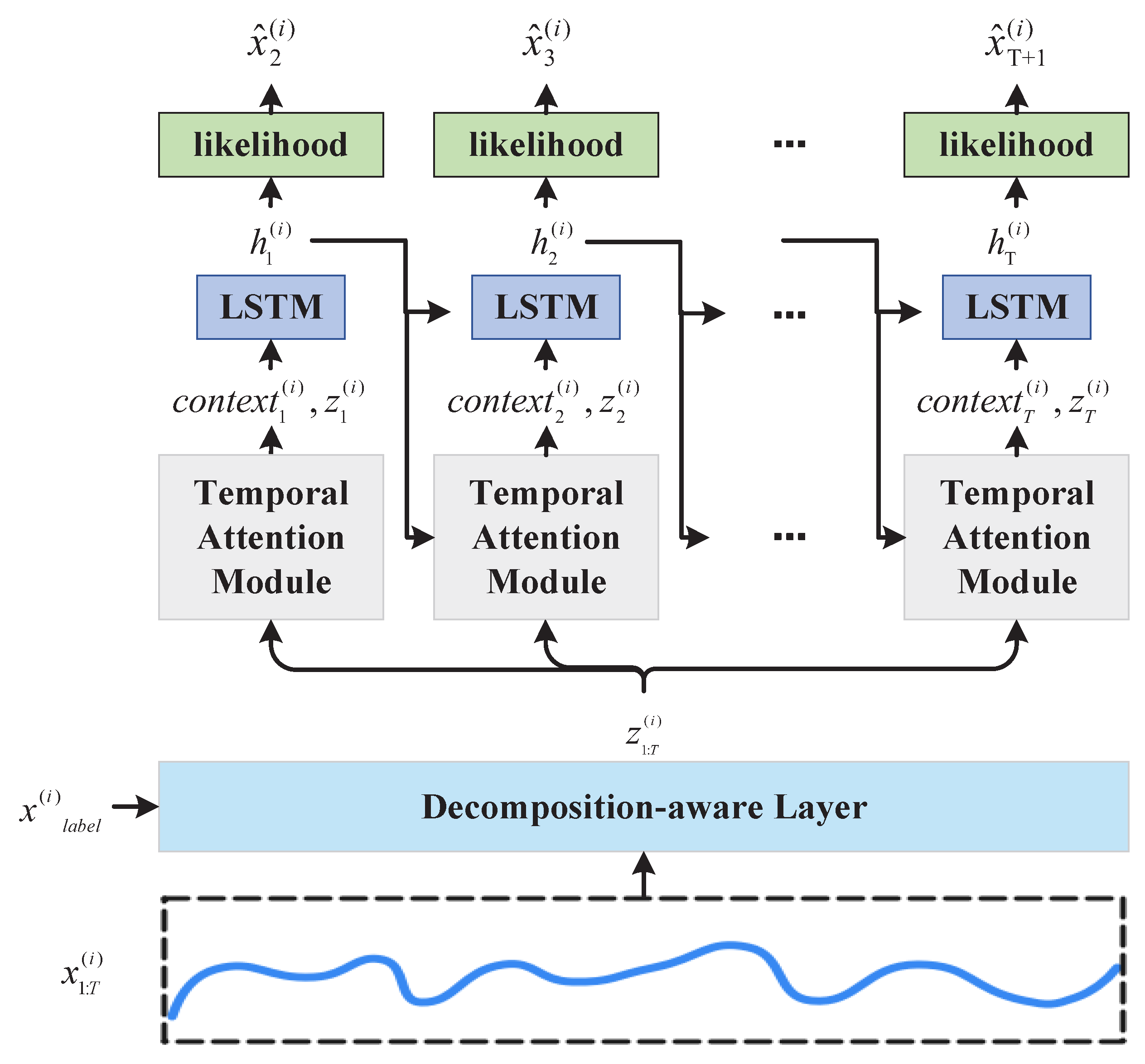
The overall structure of the model is shown in Figure 1. The time series $x_{1:T}^{\left(i\right)}$ is first passed through a decomposition-aware layer to extract the global and local features, generating a decomposed feature representation $z_{1:T}^{\left(i\right)}$. Then, at each time step t, the context vector ${\mathrm{context}}_t^{\left(i\right)}$ for the current time step is generated using a temporal attention module. This module takes the decomposed global feature $z_{1:T}^{\left(i\right)}$ and the hidden state from the previous time step $h_{t-1}^{\left(i\right)}$ as inputs, computes the attention weights, and aggregates the historical information from $z_{1:T}^{\left(i\right)}$ that is relevant to the current prediction task. The context vector ${\mathrm{context}}_t^{\left(i\right)}$, together with the decomposed feature for the current time step $z_t^{\left(i\right)}$, is then passed to an LSTM module, generating the hidden state $h_t^{\left(i\right)}$ for the current time step. The hidden state $h_t^{\left(i\right)}$ is further passed to a likelihood function module, which computes the output distribution parameters (mean ${\mu }_t^{\left(i\right)}$ and variance ${\sigma }_t^{\left(i\right)}$), from which the predicted value for the next time step ${\widehat{x}}_{t+1}^{\left(i\right)}$ is generated. This recursive process progressively updates the hidden state and context information at each time step, enabling the model to dynamically focus on the historical information relevant to the current prediction, thereby achieving precise modeling and forecasting for different time series.

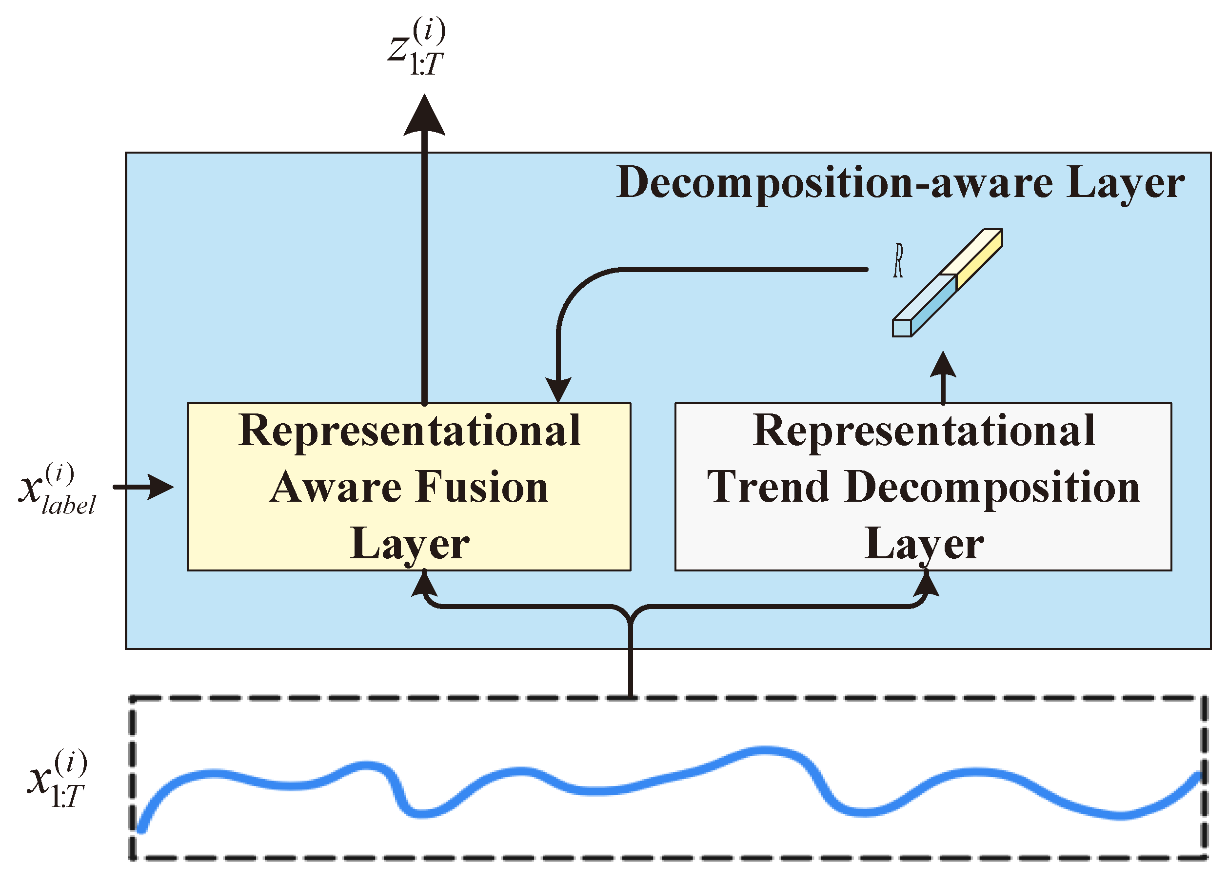
3.2. The Decomposition-Aware Layer

We propose a representation-aware decomposition layer, which consists of a representation-aware trend decomposition layer and a representation-aware fusion layer, as shown in Figure 2. First, the time series $x_{1:T}^{\left(i\right)}$ is passed through the representation-aware trend decomposition layer to obtain a representation R. Then, the time series $x_{1:T}^{\left(i\right)}$, the representation R, and the label information $x_{\mathrm{label}}^{\left(i\right)}$ of the time series are fed into the representation-aware fusion layer to generate the final representation of the temporal features $z_{1:T}^{\left(i\right)}$.

3.2.1. Representation-Aware Trend Decomposition Layer

To handle various time series inputs, we need to learn and process different time series in the same model. Therefore, we use the representation-aware trend decomposition layer to capture the internal trend features of different time series, for which a representation-aware trend decomposition indicator vector is generated to represent their respective characterization category information.

These indicator vectors effectively distinguish different feature types and capture the temporal correlations among similar representations, thus enhancing the model’s ability to recognize different feature categories.

By decomposing the global and local trends, the model captures the long-term trends and short-term dynamics of the time series, enhancing its representation capacity and predictive accuracy. The global trend features are extracted through specially designed convolutional layers, helping the model understand macro-level patterns, while the local trend features are adjusted via learnable frequency-domain transformations and restored to the time domain to capture the short-term dynamics and fine-grained variations.

Specifically, the time series data are first decomposed using convolutional kernels. For each time series, both the global and local trend features are extracted. As shown in Figure 3, the representation-aware trend decomposition block decomposes the original time series using a global trend decomposer and a local trend decomposer to build the global and local trend features. After decomposition, the model uses a linear mapping layer to map the global and local trend features, resulting in the representation-aware trend decomposition indicator vector R.

(1)

The Global Trend Decompositor

Refer to Figure 3. To enable the model to adapt to diverse input data, the global trend decompositor consists of T 2D convolutional layers, where T represents the number of time steps in the input sequence. Each convolution layer is designed to capture the long-term trend features of the input sequence, helping the model to understand and decompose the global information.

The global trend decompositor aims to extract long-term trend features from the input sequence, enhancing the model’s ability to handle complex data variations. The module is composed of L 2D convolutional layers, each of which progressively processes the input data to extract and strengthen the trend features. In each layer, the input $G^{j-1}$ is processed through a 2D convolution operation and an activation function tanh, producing the output $G^j$:

$$G^j=tanh({\mathrm{Conv}}_2(G^{j-1})),j\in \{1,2,\cdots ,L\}$$

(2)

where the initial input $G^0=x_{1:T}^{\left(i\right)}$. This process is repeated across L convolution layers, gradually extracting rgw long-term trend features. The final global trend feature is the output of the last layer: $S^T=G^L$. This multi-layer convolution design effectively captures the overall trend in the input sequence, allowing the model to understand the evolution of the time series data at a global scale.

(2)

The Local Trend Decompositor

The local trend decompositor, as shown in Figure 3, primarily captures the short-term local changes in the input data to obtain more detailed feature representations. First, a Fast Fourier Transform (FFT) transforms the input sequence into the frequency domain. This operation enables the model to analyze and process the signal more efficiently in the frequency domain.

A learnable element-wise linear layer is applied in the frequency domain, performing adaptive transformations on each frequency component. This layer contains independent complex-valued parameters, assigning different weights and phase shifts to each frequency, enhancing the model’s expressive power. After the frequency-domain transformation, an Inverse FFT converts the adjusted frequency representation back into the time-domain signal. This step allows the model to extract the local variation features, denoted as the local trend $S_P$, capturing the short-term dynamics in the data:

$$S^P=\mathrm{IFFT}\left(\mathrm{Linear}\right(\mathrm{FFT}(x_{1:T}^{\left(i\right)})\left)\right)$$

(3)

(3)

Global/Local Mapping and Merging

After applying the global trend decompositor and the local trend decompositor, we obtain the global trend $G^T$ and the local trend $S^P$. These are then passed through a linear mapping layer and concatenated to form the final representation $R\in {\mathbb{R}}^{T\times d_R}$:

$$R=\mathrm{concat}(\mathrm{FC}(S^T),\mathrm{FC}(S^P))$$

(4)

By merging the global and local features, the representation-aware trend decomposition module can capture both the long-term and short-term dynamics in the input data, providing a multi-dimensional, fine-grained feature representation for further processing in the subsequent representation-aware fusion layer. This processing ensures that the model can effectively handle a wide range of complex time series data inputs, even without explicit category labels.

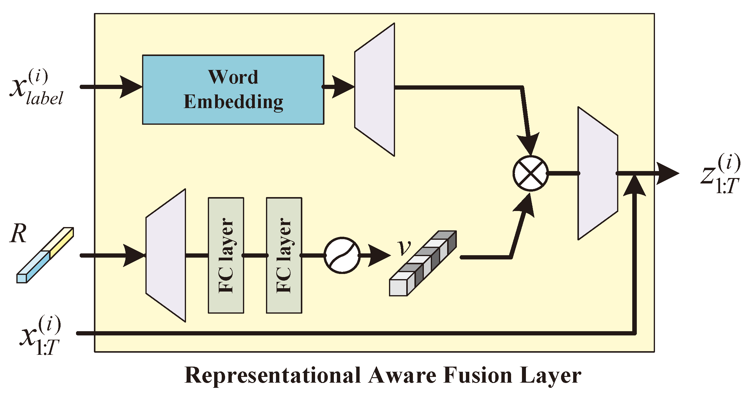
3.2.2. Representation-Aware Fusion Layer

Existing networks suitable for discriminating various features often directly concatenate the categorical feature information and time series features before feeding them into the model. However, because there are domain differences between categorical representations and time series features, directly using convolutions to process them together may introduce interference. To address these issues, we design a representation-aware fusion layer, which merges the representation R obtained from the trend decomposition layer and the adjustment parameters $F_1$ generated from the labels. This layer leverages both the trend decomposition vectors and the label information to adapt to specific time series inputs and mitigate the domain gap between the categorical and temporal features. Specifically, $F_1$ acts as a modulator that adjusts the representation R by dynamically emphasizing relevant feature dimensions and suppressing irrelevant ones. This adaptive fusion mechanism ensures that the model captures the interplay between categorical and temporal features better.

Furthermore, the representation-aware fusion layer introduces a learnable transformation matrix to project the fused representation into a unified latent space, aligning features from different domains. This step reduces the domain interference and enhances the model’s ability to discriminate between feature categories. By learning context-aware adjustments, the fusion layer enables the model to effectively differentiate and process inputs with diverse temporal and categorical characteristics, ultimately improving the performance in multivariate time series forecasting tasks.

Refer to Figure 4. The label information $X_{\mathrm{label}}$ is first transformed into a dense vector representation via word embeddings “WE” to express it in a broader feature space. The introduction of the embedding matrix enables the capture of the semantic relationships between labels while reducing the impact of label sparsity. To further enhance the feature expression, the vector generated by the word embeddings is expanded in its feature dimension through a high-dimensional linear mapping layer $F_{\mathrm{up}}$, resulting in the modulation parameters $F_1$:

$$F_1=F_{\mathrm{up}}\left(\mathrm{WE}\left(X_{\mathrm{label}}\right)\right)$$

(5)

where $F_1\in {\mathbb{R}}^{T\times d_{\mathrm{label}}}$ represents the expanded label modulation parameters. This process maps the label information from a low-dimensional space to a high-dimensional space that aligns with the representation features, thus laying the foundation for subsequent dynamic modulation.

The input representation-aware trend decomposition indicator vector R undergoes processing using an upsampling layer to further amplify the key information within the representation:

$$R^{\prime }=R_{\mathrm{up}}\left(R\right)$$

(6)

where $R^{\prime }\in {\mathbb{R}}^{T\times d_{\mathrm{label}}}$ represents the amplified representation with an increased resolution, ensuring that critical features are more finely extracted and providing high-quality input for subsequent dynamic weighting.

The amplified representation $R^{\prime }$ is processed through two fully connected layers, followed by ReLU and sigmoid activation functions, generating the dynamic weighting mask $v\in {\mathbb{R}}^{T\times d_{\mathrm{label}}}$:

$$v=\mathrm{sigmoid}\left(FC\left(ReLU\left(FC\right(R’\left)\right)\right)\right)$$

(7)

where $v\in {\mathbb{R}}^{T\times d_{\mathrm{label}}}$ is the dynamic weighting mask. The purpose of v is to assign weights to the importance of different features, giving higher weights to the critical representations and guiding the model to focus on the most meaningful features.

By adjusting the importance of different features, the mask v enhances the model’s performance in multi-representational tasks. The dynamic weighting mask v is used to modulate the label-generated parameters $F_1$, producing the modulated feature representation $F_2\in {\mathbb{R}}^{T\times d_{\mathrm{label}}}$:

$$F_2=F_1\times v$$

(8)

Finally, the modulated features $F_2$ undergo downsampling via the $F_{\mathrm{down}}$ layer and are added to the original input sequence $x_{1:T}^{\left(i\right)}$ through a residual connection to generate the final output $z_{1:T}^{\left(i\right)}\in {\mathbb{R}}^{T\times d_{\mathrm{out}}}$:

$$z_{1:T}^{\left(i\right)}=F_{\mathrm{down}}\left(F_2\right)+x_{1:T}^{\left(i\right)}$$

(9)

This method enables precise modulation of multi-representational features by passing the label information through word embeddings and high-dimensional mapping to generate modulation parameters and combining them with the dynamically generated weighting mask. It effectively enhances the model’s ability to focus on key representations while maintaining the integrity of the global structure through the residual connection, providing an efficient modeling framework for multi-representational tasks.

3.3. The Temporal Attention Module

Traditional LSTMs often struggle with long-term dependencies due to the limitations in their memory mechanisms, leading to the loss of crucial information over extended time periods and difficulty in precisely identifying the most important time steps for the current predictions. To address this issue, the model design incorporates a temporal attention module (TAM), which dynamically assigns weights to historical time steps. This allows the model to automatically focus on the time points most relevant to the current decision at each prediction step. The mechanism works by calculating the correlation weights between time steps and dynamically adjusting the influence of different historical time steps, effectively mitigating the problem of long-term dependency loss and significantly improving the performance in long-sequence prediction tasks.

As shown in Figure 5, in this architecture, the temporal attention module receives the hidden state of the previous time step, $h_{t-1}^{\left(i\right)}$, passed down from the upper-layer LSTM, and $z_{1:T}^{\left(i\right)}$, obtained through the decomposition-aware layer, and computes the attention weights ${\beta }_t^{1,\left(i\right)},{\beta }_t^{2,\left(i\right)},\cdots ,{\beta }_t^{T,\left(i\right)}$ for each time step. The attention mechanism calculates the raw attention scores for each hidden state, which are then transformed into weights using a softmax function. This enables the model to automatically identify the historical time steps that are most crucial to the current prediction.

Ultimately, the model computes the context vector for the current time step ${\mathrm{context}}_t^{\left(i\right)}$ by performing a weighted sum of all historical hidden states according to their attention weights: ${\mathrm{context}}_t^{\left(i\right)}={\sum }_{j=1}^T{\beta }_t^{j,\left(i\right)}·h_j^e$. This context vector serves as an important input for the current prediction. The attention mechanism improves the model’s precision in predicting the long-term dependencies and improves interpretability, allowing us to understand which historical moments the model is focused on the most during the prediction process.

3.4. Probabilistic Prediction

The traditional models for time series prediction typically focus on directly generating specific numerical values at a given time step, without fully accounting for the uncertainty present in the data. While such models can predict future trends or outcomes to some extent, they often struggle to maintain high accuracy when dealing with complex time series data characterized by significant noise or uncertainty. To address this limitation, we extend the temporal attention module and adopt an LSTM-based framework similar to DeepAR, incorporating probabilistic forecasting to enhance modeling the uncertainty in future trends. The overall framework is shown in Figure 1.

To predict future time series data ${\widehat{x}}_{T+1:T+\tau }^{\left(i\right)}$, we model the conditional probability based on historical data $x_{1:T}^{\left(i\right)}$ using past time series to forecast the future. The model’s goal is to predict the probability distribution of the time series ${\widehat{x}}_{t+1:t+\tau }^{\left(i\right)}$ given the historical data $x_{t-T+1:t}^{\left(i\right)}$:

$$P\left({\widehat{x}}_{T+1:T+\tau }^{\left(i\right)}\mid x_{1:T}^{\left(i\right)}\right)$$

(10)

To achieve probabilistic forecasting based on likelihood functions, the model adopts an LSTM decoder structure, making predictions step by step. At each time step, the decoder outputs a hidden state $h_t^{\left(i\right)}$, which is then passed through a likelihood estimation layer to calculate the probability distribution for the next time step’s predicted value. This approach generates point predictions (e.g., mean values) and provides a measure of uncertainty by outputting the complete probability distribution, thereby enhancing the model’s expressiveness. The core update formula for the LSTM decoder is the following:

$$h_t^{\left(i\right)}=\mathrm{LSTM}\left(h_{t-1}^{\left(i\right)},[{\mathrm{context}}_t,z_t^{\left(i\right)}],\theta \right),h_t^{\left(i\right)}\in {\mathbb{R}}^{T\times d_{\mathrm{hidden}}}$$

(11)

where $\theta$ represents the model parameters, $h_t^{\left(i\right)}$ is the hidden state at time step t, $h_{t-1}^{\left(i\right)}$ is the hidden state from the previous time step, and ${\mathrm{context}}_t$ is the context vector output from the temporal attention module. The model gradually predicts the future values based on past outputs through this recursive process, leveraging historical data and attention-modulated context vectors to improve the forecast.

By incorporating probabilistic forecasting into the LSTM framework and leveraging the temporal attention module, the model improves its predictive accuracy for time series with high noise or uncertainty and enhances the interpretability by providing full probability distributions that reflect the uncertainty of the future predictions.

At each time step, the hidden state $h_t^{\left(i\right)}$ is passed to the likelihood estimation layer, which generates the probability distribution for the predicted value. Using the probability distribution as the output, the model predicts the expected future values (e.g., the mean) and provides a measure of uncertainty, such as the variance or confidence intervals. The decoder predicts in a stepwise recursive manner, where the predicted value at the current time step is used as the input for subsequent time steps. This approach allows the model to leverage historical information and past prediction results, making the future value predictions more accurate and robust. The optimization goal is typically to maximize the likelihood function, train the model to generate predictions closer to the true distribution, and improve its ability to model uncertainty. This design enhances the model’s adaptability and expressive power for complex time series data, going beyond point predictions to offer a more comprehensive understanding of future trends and their associated uncertainties.

Likelihood Function

The likelihood function $\mathsf{\ell }\left(x\right|\theta )$ determines the “noise model”, and the choice of the likelihood function depends on its compatibility with the statistical properties of the data [22]. Since the predicted sequence consists of continuous numerical values, we consider a Gaussian likelihood function for real-valued data. The parameters $\theta$ are directly predicted by the network, such as the mean and variance in the probability distribution at the next time step. The Gaussian likelihood function is defined as follows:

$${\mathsf{\ell }}_G\left(x\right|\mu ,\sigma )={\displaystyle \frac{1}{\sqrt{2\pi {\sigma }^2}}}exp\left(-{\displaystyle \frac{{(x-\mu )}^2}{2{\sigma }^2}}\right)$$

(12)

where $\mu$ and $\sigma$ represent the mean and variance, respectively. The model parameters $\theta =(\mu ,\sigma )$, where the mean $\mu$ is obtained from the decoder’s output hidden state $h_t^{\left(i\right)}$ through a linear layer:

$${\mu }_t={\mathbf{w}}_{\mu }^T{h}_t^d+b_{\mu }$$

(13)

To ensure the variance $\sigma$ is greater than zero, the Softplus activation function is applied to the decoder’s output hidden state $h_t^{\left(i\right)}$ after a linear transformation:

$${\sigma }_t=log(1+exp({\mathbf{w}}_{\sigma }^T{h}_t^d+b_{\sigma }))$$

(14)

This formulation ensures that ${\sigma }_t$ remains positive, allowing the model to predict both the mean and variance for each time step, thus providing a complete probabilistic forecast.

3.5. Objective Loss

For the entire time series dataset $\mathbf{X}=\{x_{1:T}^{\left(i\right)}\mid i=1,2,\dots ,N\}$, where $x_{1:T}^{\left(i\right)}$ represents the i-th time series, the model’s objective is to learn the distribution of each time series and optimize the parameters by maximizing the log-likelihood function during training.

The input to the model is each time series $x_{1:T}^{\left(i\right)}$, and the output is the predicted values ${\widehat{x}}_{2:T+1}^{\left(i\right)}$. For the entire dataset, the objective is to maximize the joint log-likelihood function of all time series:

$$L=\sum _{i=1}^N\sum _{t=2}^{T+1}log{\mathsf{\ell }}_G\left(x_t^{\left(i\right)}\mid {\mu }_t^{\left(i\right)},{\sigma }_t^{\left(i\right)}\right)$$

(15)

where

$${\mathsf{\ell }}_G\left(x_t^{\left(i\right)}\mid {\mu }_t^{\left(i\right)},{\sigma }_t^{\left(i\right)}\right)={\displaystyle \frac{1}{\sqrt{2\pi {\left({\sigma }_t^{\left(i\right)}\right)}^2}}}exp\left(-{\displaystyle \frac{{(x_t^{\left(i\right)}-{\mu }_t^{\left(i\right)})}^2}{2{\left({\sigma }_t^{\left(i\right)}\right)}^2}}\right),$$

(16)

is the Gaussian probability density function for the i-th time series at time step t. By maximizing the log-likelihood function, we aim to find a set of parameters that maximize the probability of the observed data under these parameters. Therefore, in practice, we need to minimize the negative log-likelihood loss $-L$ over the entire dataset during training. This approach ensures that the model learns the parameters that capture the observed time series data distribution best.

4. The Experimental Setup

4.1. Implementation Details

Our model is implemented using Python 3.8 and PyTorch 1.10 and trained on an NVIDIA RTX 3060 GPU. During training, we use a batch size of 512, with the Adam optimizer and a learning rate of 0.001. In this experiment, we set the key parameters for the model and validated its performance across several baseline models.

The window size L for global trend decomposition is set to 6, capturing the long-term trend information from the time series. The dimensionality $d_R$ of the representation vector generated after global trend decomposition is set to 8, further enhancing the feature expressiveness. The word embedding dimension $d_{\mathrm{label}}$ for the labels is set to 16, while the final output dimension $d_{\mathrm{out}}$ is set to 32. In the temporal attention module, the hidden state dimension $d_{\mathrm{hidden}}$ of the LSTM is set to 16, ensuring efficient encoding of the temporal dependencies. For the decoding process, the LSTM hidden state dimension for output prediction is set to 32, providing a sufficient capacity to generate accurate predictions. Finally, the time prediction window T is set to 6.

For each time point t, we use the predicted ${\mu }_t^{\left(i\right)}$ and ${\sigma }_t^{\left(i\right)}$ to perform 500 samplings and compute ${\widehat{x}}_t^{\left(i\right),\rho }$, as described in Section 4.4 for the ROU metric. To minimize the impact of randomness, we repeat the sampling process 10 times for all experiments. The results are reported as the mean value with ± ranges representing the variability across repetitions, which are shown in the tables for all metrics.

4.2. Open Datasets

To verify our model’s ability to handle a wide range of different features, we conducted experiments on the CMAPSS and OZONE datasets to assess its applicability and robustness in dealing with various features.

4.2.1. CMAPSS Dataset

The CMAPSS dataset [23] contains time series data from multiple aircraft engine sensors and is widely used for predicting the Remaining Useful Life (RUL) of equipment. In this experiment, 14 time series were selected, including sensors s2–s4, s7–s9, s11–s15, s17, and s20–s21 [24,25,26].

4.2.2. OZONE Dataset

The OZONE dataset [27] records the variation in atmospheric ozone concentrations, including time series data from various meteorological and pollutant variables, used to predict future ozone concentration changes. The data, collected between 1998 and 2004 in Houston, Galveston, and Brazoria, Texas, are divided into two subsets, an 8 h peak dataset (eighthr) and a 1 h peak dataset (onehr), recording the ozone concentration peaks over these periods. For modeling and analysis, 12 representative time series variables are selected, including wind speed (WSR_PK, WSR_AV), temperature (T_PK, T_AV), humidity (RH50), altitude (HT70, T50), wind direction (U50, V50), pollutant index (KI), total atmospheric pressure (SLP), and other relevant meteorological indicators (TT). The training phase uses the 8 h peak dataset, while the testing phase uses the 1 h peak dataset to evaluate the model’s generalization performance across different time granularities. The experiment focuses on predicting the future ozone concentration trends using meteorological and pollutant variables.

All of the selected time series data exhibit significant nonlinear trends, long-term dependencies, and noise interference, making them suitable for model validation. All of the input data are normalized to the range [−1, 1] to ensure consistency in the numerical scale across features, preventing training instability due to dimensional differences.

4.3. Our Electronic System Dataset

The key characteristics selected for sampling should reflect the operational state of an electronic system, thereby facilitating reasonable health assessments. Embedded computers, being the core of equipment electronic systems, are used as an illustrative example to explain the selection of the key characteristics. The parameters of these characteristics must scientifically reflect the reliability requirements under various conditions and comprehensively and reasonably represent the health status of the control computer. Each indicator should be relatively independent to avoid mutual influence. Key characteristic parameters should be effectively measurable and statistically quantifiable, facilitating comparisons and contrasts that can demonstrate the overall degradation trend in the electronic system [28].

Through a simplified analysis of the entire electronic system, as shown in Figure 6, the following key characteristic parameters were identified for the degradation of the whole system, and the data scale is shown in

Table 1. Description of the electronic system dataset.

Index	Feature	Sequence Length	Number of Sequences
1	DA	640	5
2	AD	640	5
3	Optocoupler	640	5
4	Clock Oscillator	640	5
5	Overall System Power	640	5

:

• Clock oscillator: The minimum system of the flight control computer primarily consists of DSP circuits, FPGA circuits, reset circuits, storage circuits, and clock circuits. Experimental findings indicate that the oscillator within the clock circuit shows a more pronounced degradation trend than the other components. Given that the oscillator serves as the time reference for the entire system, degradation of its parameters can affect the timing sequence of the system operations.
• Analog signals (AD/DA): Analog signals include both AD acquisition and DA output. Analysis of the data obtained from natural storage, accelerated storage, and the products returned after overhaul indicates that analogue signal parameters show a more noticeable degradation trend with increasing storage time.
• Optocouplers: Taking differential RS422 communication as an example, the transmitter uses a differential output chip, while the receiver employs an optocoupler for isolation. Changes in the optocoupler’s parameters and the interface crystal oscillator’s degradation can both affect the communication waveform’s baud rate, leading to data transmission errors.
• Overall system power: Over extended periods, the leakage current across various components in the system gradually increases. Under prolonged working conditions, the working current and voltage increase, leading to a higher power consumption. This increased power consumption can reflect the degradation trend in the entire system, making it a key characteristic parameter for assessing the degradation of the system.

4.4. Evaluation Metrics

We use the Root Mean Squared Error (RMSE), the Relative Root Mean Square Error (RRMSE), Normalized Deviation (ND), and the ROU metric to comprehensively evaluate the model’s prediction performance and ability to model uncertainty. The RMSE, RRMSE, and ND are commonly used to assess the performance of time series forecasting algorithms, while the ROU is used to evaluate the coverage of the probabilistic prediction intervals. The definitions of these metrics are as follows:

RMSE for the i-th time series:

$${\mathrm{RMSE}}^{\left(i\right)}=\sqrt{{\displaystyle \frac{1}{S}}\sum _{j=1}^S{(x_j^{\left(i\right)}-{\widehat{x}}_j^{\left(i\right)})}^2}$$

(17)

RRMSE for the i-th time series:

$${\mathrm{RRMSE}}^{\left(i\right)}={\displaystyle \frac{\sqrt{\frac{1}{S}{\sum }_{j=1}^S{\left(x_j^{\left(i\right)}-{\widehat{x}}_j^{\left(i\right)}\right)}^2}}{{\overline{x}}^{\left(i\right)}}},{\overline{x}}^{\left(i\right)}={\displaystyle \frac{{\sum }_{j=1}^S{x}_j^{\left(i\right)}}{S}}$$

(18)

ND for the i-th time series:

$${\mathrm{ND}}^{\left(i\right)}={\displaystyle \frac{{\sum }_{j=1}^S|x_j^{\left(i\right)}-{\widehat{x}}_j^{\left(i\right)}|}{{\sum }_{j=1}^S\left|x_j^{\left(i\right)}\right|}}$$

(19)

ROU for the i-th time series at a quantile $\rho$:

$${\mathrm{ROU}}_{\rho }^{\left(i\right)}={\displaystyle \frac{{\sum }_{j=1}^S{L}_{\rho }(x_j^{\left(i\right)},{\widehat{x}}_j^{\left(i\right),\rho })}{{\sum }_{j=1}^S{x}_j^{\left(i\right)}}}$$

(20)

where S is the total number of test samples for the i-th time series, $x_j^{\left(i\right)}$ is the true value at the j-th test sample, and ${\widehat{x}}_j^{\left(i\right)}$ is the predicted value. $L_{\rho }(x_j^{\left(i\right)},{\widehat{x}}_j^{\left(i\right),\rho })$ represents the quantile loss, which measures the deviation between the predicted quantile and the true value:

$$L_{\rho }(x_j^{(i)},{\widehat{x}}_j^{(i),\rho })=2({\widehat{x}}_j^{(i),\rho }-x_j^{(i)})(\rho ·I({\widehat{x}}_j^{(i),\rho }>x_j^{(i)})-(1-\rho )·I({\widehat{x}}_j^{(i),\rho }\le x_j^{(i)}))$$

(21)

where ${\widehat{x}}_j^{\left(i\right),\rho }$ represents the predicted quantile value for the j-th sample in the i-th time series, corresponding to the quantile $\rho$. This value is determined based on the sampling distribution generated using the predicted mean ${\widehat{\mu }}_j^{\left(i\right)}$ and variance ${\widehat{\sigma }}_j^{\left(i\right)}$. It reflects the $\rho$-quantile of the predictive distribution. The Indicator Function $I(·)$ is evaluated as 1 if the specified condition is satisfied; otherwise, it is evaluated as 0.

To obtain the overall performance across the entire dataset, the average of the metrics across all of the time series in the dataset is calculated:

$$\begin{array}{cc}\hfill \mathrm{RMSE}& ={\displaystyle \frac{1}{N}}\sum _{i=1}^N{\mathrm{RMSE}}^{\left(i\right)},\mathrm{RRMSE}={\displaystyle \frac{1}{N}}\sum _{i=1}^N{\mathrm{RRMSE}}^{\left(i\right)},\hfill \\ \hfill \mathrm{ND}& ={\displaystyle \frac{1}{N}}\sum _{i=1}^N{\mathrm{ND}}^{\left(i\right)},{\mathrm{ROU}}_{\rho }={\displaystyle \frac{1}{N}}\sum _{i=1}^N{\mathrm{ROU}}_{\rho }^{\left(i\right)}\hfill \end{array}$$

(22)

where N is the total number of time series in the dataset. By performing independent tests for each time series and calculating the overall metrics, we can comprehensively evaluate the model’s prediction performance and ability to model uncertainty for the CMAPSS and OZONE datasets.

4.5. Results and Analysis

4.5.1. Comparison with Other Models

To validate the effectiveness of the proposed method, we perform a comprehensive comparison on the CMAPSS and OZONE time series datasets with four baseline models and two additional diffusion-based probabilistic models. These baseline models include an RNN [29], LSTM [30], DaRNN [8], and DeepAR [22], which represent traditional time series modeling, extensions of recurrent neural networks, attention-based modeling, and state-of-the-art probabilistic-distribution-based modeling methods, respectively. In addition, we include two diffusion-based probabilistic models, CSDI [31] and TSDiff [32], to further demonstrate the versatility and robustness of the proposed method.

CMAPSS: 

Table 2. Performance comparison of our proposed method on the CMAPSS test datasets.

	Metrics	ND	RMSE	RRMSE	ROU50	ROU90	ROU95
Model
RNN [29]		0.366 $\pm 0.02$	0.457 $\pm 0.03$	0.598 $\pm 0.04$	-	-	-
LSTM [30]		0.376 $\pm 0.03$	0.441 $\pm 0.02$	0.501 $\pm 0.01$	-	-	-
DaRNN [8]		0.156 $\pm 0.02$	0.236 $\pm 0.01$	0.305 $\pm 0.03$	-	-	-
DeepAR [22]		0.223 $\pm 0.03$	0.382 $\pm 0.04$	0.449 $\pm 0.02$	0.109 $\pm 0.01$	0.244 $\pm 0.02$	0.120 $\pm 0.03$
CSDI  [31]		0.062 $\pm 0.02$	0.074 $\pm 0.03$	0.081 $\pm 0.01$	0.094 $\pm 0.04$	0.067 $\pm 0.02$	0.054 $\pm 0.03$
TSDiff [32]		0.056 $\pm 0.03$	0.068 $\pm 0.01$	0.059 $\pm 0.02$	0.057 $\pm 0.04$	0.033$\pm 0.02$	0.042 $\pm 0.03$
Ours		0.040$\pm 0.01$	0.051$\pm 0.02$	0.067$\pm 0.03$	0.040$\pm 0.01$	0.060$\pm 0.02$	0.037$\pm 0.03$

ROU50, ROU90, and ROU95 represent the evaluation of the probabilistic prediction intervals at different quantiles. The best results are shown in bold in the table.

presents the experimental results on the CMAPSS dataset, demonstrating that our model outperforms the RNN, LSTM, DeepAR, CSDI, and TSDiff across all metrics. The RNN and LSTM exhibit similar ND scores (0.366 and 0.376) and RMSE scores (0.457 and 0.441), reflecting their limitations in capturing long-term dependencies. DeepAR improves the distribution coverage but still performs worse in terms of the ND (0.223) and RMSE (0.382). The diffusion-based models, CSDI and TSDiff, demonstrate significant improvements. CSDI achieves ND and RMSE scores of 0.062 and 0.074, while TSDiff outperforms it with an ND of 0.056, an RMSE of 0.068, and the best interval coverage (ROU90 of 0.033).

In contrast, our model achieves an ND of 0.04, an RMSE of 0.051, and an RRMSE of 0.067, showing a clear advantage over the baseline models. Additionally, it achieves ROU50 and ROU90 values of 0.040 and 0.060, respectively, indicating that the generated confidence intervals are more accurate. The superior performance of our model can be attributed to several key factors: The decomposition-aware layer effectively extracts both the long-term trends and short-term variations; the temporal attention module dynamically focuses on critical time steps, avoiding interference from irrelevant global features; and the Gaussian-based prediction method further enhances the uncertainty modeling, leading to more precise and robust forecasting results.

OZONE: The experimental results on the OZONE dataset, as shown in

Table 3. Performance comparison of our proposed method on the OZONE onehr datasets.

	Metrics	ND	RMSE	RRMSE	ROU50	ROU90	ROU95
Model
RNN [29]		0.395 $\pm 0.03$	0.514 $\pm 0.02$	0.223 $\pm 0.04$	-	-	-
LSTM [30]		0.421 $\pm 0.02$	0.523 $\pm 0.04$	0.215 $\pm 0.01$	-	-	-
DaRNN [8]		0.208 $\pm 0.01$	0.295 $\pm 0.02$	0.112 $\pm 0.03$	-	-	-
DeepAR [22]		0.189 $\pm 0.04$	0.374 $\pm 0.03$	0.171 $\pm 0.02$	0.104 $\pm 0.01$	0.225 $\pm 0.02$	0.087 $\pm 0.03$
CSDI  [31]		0.086 $\pm 0.02$	0.093 $\pm 0.03$	0.041 $\pm 0.01$	0.082 $\pm 0.04$	0.047 $\pm 0.02$	0.029 $\pm 0.03$
TSDiff [32]		0.081 $\pm 0.03$	0.079$\pm 0.01$	0.036 $\pm 0.02$	0.071$\pm 0.04$	0.051 $\pm 0.03$	0.032 $\pm 0.02$
Ours		0.072$\pm 0.01$	0.085 $\pm 0.02$	0.034$\pm 0.03$	0.073 $\pm 0.01$	0.040$\pm 0.02$	0.026$\pm 0.03$

ROU50, ROU90 and ROU95 represent the evaluation of the probabilistic prediction intervals at different quantiles. The best results are shown in bold in the table.

, demonstrate the superior performance of our model compared to that of the baseline methods. Traditional models like the RNN and LSTM exhibit limited capabilities, with ND values of 0.395 and 0.421, respectively. DaRNN improves in its performance with an ND of 0.208. DeepAR achieves moderate enhancements, with an ND of 0.189 and an ROU90 of 0.225, showing reasonable probabilistic predictions. The diffusion-based models, CSDI and TSDiff, further advance the performance, with TSDiff achieving an ND of 0.081 and an ROU90 of 0.051. Our model outperforms all of the baselines, achieving the best ND of 0.072 and ROU90 of 0.040, effectively capturing the dynamic variations and nonlinear relationships in multivariate time series.

In contrast, our model achieves ND and RMSE and RRMSE values of 0.072, 0.085, and 0.034, respectively, on the OZONE dataset, alongside ROU50 and ROU90 values of 0.073 and 0.040. These results highlight the model’s superior capability in uncertainty modeling. By incorporating a decomposition-aware layer and attention-based feature aggregation, our model effectively captures critical dynamic variations in multivariate time series, particularly when dealing with nonlinear relationships among variables and noise interference.

4.5.2. Results of Our Proposed Model on Our Electronic System Dataset

Table 4. Performance metrics for individual features and overall results on our electronic system test datasets.

Feature	ND	RMSE	RRMSE	ROU50	ROU90
DA	0.013	0.016	0.007	0.023	0.013
AD	0.011	0.014	0.007	0.023	0.011
Optocoupler	0.010	0.012	0.006	0.023	0.010
Clock Oscillator	0.010	0.012	0.007	0.023	0.010
Overall System Power	0.010	0.013	0.007	0.023	0.010
Total	0.011	0.014	0.007	0.023	0.011

The best results are shown in bold in the table.

presents the experimental results of our model on our electronic system dataset. The table includes the prediction metrics for multiple key features, as well as overall performance indicators. Specifically, our model achieved an ND of 0.011 and an RMSE of 0.014, demonstrating high prediction accuracy. Additionally, the model performed excellently in uncertainty modeling, with ROU50 and ROU90 values of 0.023 and 0.011, respectively, indicating more precisely generated confidence intervals. The superior performance of the model can be attributed to the multi-scale feature extraction mechanism, which effectively captures long-term trends and short-term fluctuations; the adaptive attention mechanism, which enhances the focus on critical time steps and improves the prediction accuracy; and the Gaussian-based prediction method, which further enhances the robustness and reliability of uncertainty modeling. These results demonstrate that our model has significant advantages in handling complex time series data.

4.5.3. Ablation Studies

To further validate the contribution of different modules to the model’s overall performance, we conducted two sets of ablation experiments on the OZONE dataset: one by removing the decomposition-aware layer and the other by removing the temporal attention module. By comparing the results of the complete model with those of the models without these modules, we analyzed the role of each module in enhancing the prediction accuracy and uncertainty modeling.

At the same time, we also validated the effectiveness of the scalability of our model with experiments involving an increasing number of time series variables. The results demonstrate that our method consistently improves performance metrics such as the ND, RMSE, and ROU90 as the number of variables increases, showcasing its robust scalability and adaptability. Additionally, we demonstrated the specific impact of the decomposition-aware layer on the sequence through t-SNE visualization, where the layer effectively improves the separability of the clusters, making the underlying patterns in the data more distinct and interpretable.

• Validation of the effectiveness of the decomposition-aware layer: The model processes the input time series $x_{1:T}^{\left(i\right)}$ directly without extracting the long-term trends and short-term fluctuation features through decomposition. As shown in

  Table 5. Ablation study results on the OZONE onehr datasets.

  	Metrics	ND	RMSE	RRMSE	ROU50	ROU90	ROU95
  Model
  Ours		0.072$\pm 0.01$	0.085$\pm 0.02$	0.034$\pm 0.03$	0.073$\pm 0.01$	0.040$\pm 0.02$	0.025$\pm 0.03$
  wo-DAL		0.134 $\pm 0.02$	0.175 $\pm 0.03$	0.047 $\pm 0.04$	0.134 $\pm 0.01$	0.062 $\pm 0.02$	0.038 $\pm 0.03$
  wo-TAM		0.225 $\pm 0.03$	0.295 $\pm 0.04$	0.104 $\pm 0.02$	0.225 $\pm 0.01$	0.104 $\pm 0.03$	0.059 $\pm 0.02$

  ROU50, ROU90, and ROU95 represent the evaluation of the probabilistic prediction intervals at different quantiles. The best results are shown in bold in the table.

  , compared to the model with the decomposition-aware layer (DAL), the ND metric deteriorates from 0.072 to 0.134, and the RMSE metric increases from 0.085 to 0.175. Additionally, the ROU90 and ROU50 metrics also experience significant declines. The removal of the DAL significantly weakens the model’s ability to represent time series features, especially in scenarios with multiple time series. This module effectively decomposes the trend and perturbation components to extract the long-term and short-term features. Without decomposition, the model must process the raw sequences directly, leading to a reduced capability in modeling complex multivariate features and a significant decline in robustness to noise. This is reflected in the worsening ND and RMSE metrics. Moreover, the feature representations generated during decomposition help the model capture the global trends in the input sequence better. The absence of this characteristic reduces the coverage of the predictive confidence intervals for ROU90 and ROU50, highlighting a weakened ability in uncertainty modeling.
• Validation of the effectiveness of the temporal attention module: The model directly inputs the decomposed features $z_t^{\left(i\right)}$ at each time step into the LSTM without extracting contextual information through the temporal attention module (TAM). As shown in Table 5, the ND and RMSE metrics deteriorate significantly from 0.072 and 0.085 to 0.225 and 0.295, respectively, while the uncertainty modeling metrics ROU90 and ROU50 drop to 0.104 and 0.225. The removal of the TAM results in the loss of the dynamic focusing mechanism, which prevents the model from weighting the historical information based on the importance of different time steps. The attention mechanism is especially critical for the OZONE dataset, which contains multivariate time series with complex inter-variable dependencies. Without the TAM, the model relies solely on fixed time series inputs and the implicit memory mechanism of the LSTM, reducing its ability to capture the nonlinear relationships between variables. This shortcoming is directly reflected in the degraded ND and RMSE metrics. Furthermore, the attention layer typically helps the model select the most relevant time steps from historical data for future predictions. The lack of this capability diminishes the model’s ability to capture long-term and short-term dependencies, resulting in a degraded predictive performance for ROU90 and ROU50.
• Visualization of t-SNE results: Figure 7 demonstrates the t-SNE visualization results of the OZONE onehr datasets sequence before and after applying the decomposition-aware layer. In Figure 7a, the visualization of the original sequence shows overlapping clusters with less distinct boundaries, making it challenging to differentiate between different groups. After applying the decomposition-aware layer, as shown in Figure 7b, the clusters become more separated and distinguishable, reflecting clearer patterns and improved decomposition of the underlying features. This result aligns with the paper’s hypothesis, indicating that the decomposition-aware layer effectively enhances the representation learning process by disentangling key features, thereby improving the overall interpretability and separability of the data.
• Validation of the effectiveness of scalability with increasing time series variables: The experimental results demonstrate that our proposed method exhibits robust scalability as the number of time series variables increases. Specifically, as shown in

  Table 6. Performance comparison of our proposed method with varying numbers of time series variables on the OZONE onehr dataset.

  	Metrics	ND	RMSE	RRMSE	ROU50	ROU90	ROU95
  Model
  2		0.099 $\pm 0.02$	0.133 $\pm 0.03$	0.017 $\pm 0.01$	0.101 $\pm 0.02$	0.059 $\pm 0.03$	0.036 $\pm 0.02$
  4		0.081 $\pm 0.01$	0.113 $\pm 0.04$	0.094 $\pm 0.02$	0.082 $\pm 0.01$	0.048 $\pm 0.02$	0.029 $\pm 0.03$
  8		0.078 $\pm 0.02$	0.102 $\pm 0.03$	0.023$\pm 0.01$	0.078 $\pm 0.02$	0.051 $\pm 0.03$	0.032 $\pm 0.02$
  12		0.072$\pm 0.01$	0.085$\pm 0.02$	0.034 $\pm 0.03$	0.073$\pm 0.01$	0.040$\pm 0.02$	0.025$\pm 0.03$

  ROU50, ROU90, and ROU95 represent the evaluation of the probabilistic prediction intervals at different quantiles. The best results are shown in bold in the table.

  , the performance metrics, including the ND, RMSE, and ROU90, improve consistently with an increasing number of time series variables. For example, the ND reduces from 0.099 to 0.071, and the RMSE decreases from 0.1325 to 0.094 as the number of variables grows from 2 to 12. This improvement is largely attributed to the decomposition-aware layer, which effectively disentangles complex temporal patterns into trend and seasonality components. By isolating and simplifying these components, the decomposition-aware layer enhances the model’s ability to capture and leverage the additional information provided by a larger number of variables, leading to improved accuracy and a more robust performance in multivariate time series forecasting tasks.

4.5.4. Visualization of the Prediction Results

OZONE: As shown in Figure 8, the prediction results on the OZONE dataset for the onehr test set are presented, covering 12 different time series variables. For each sequence, only the first 200 test time points are displayed. Each subplot corresponds to a specific sequence, with the horizontal axis representing time (Cycle) and the vertical axis showing the normalized values. The green dashed line represents the actual values (Actual Value), the orange solid line denotes the predicted values (Predicted Value), and the orange shaded area illustrates the uncertainty range of the predictions.

The model demonstrates an excellent performance in capturing global trends. For example, in the WSR_AV and T_AV sequences, the predicted values align closely with the actual values, indicating the model’s strong ability to understand long-term trends. Similarly, the KI sequence shows a clear upward trend, with the predicted curve following the actual values, highlighting the model’s adaptability to monotonic data. In the HT70 sequence, the model successfully captures periodic fluctuations, further showcasing its ability to model time series patterns.

The model also excels at predicting local details. In sequences like SLP, it captures subtle fluctuations, reflecting its sensitivity to fine-grained features. In more complex sequences such as RH50 and TT, the model accurately reconstructs changing trends, demonstrating its strong generalization ability.

The uncertainty regions further highlight the model’s robustness. Narrow uncertainty ranges in sequences like WSR_AV, T_AV, and SLP indicate high confidence, while in more complex sequences like T_PK and V50, the model maintains high accuracy despite intricate patterns. The uncertainty regions effectively cover potential variations, showcasing the model’s adaptability.

Overall, the model excels in time series prediction, demonstrating high reliability in capturing trends, restoring details, and modeling uncertainty. These results underscore its potential for complex time series tasks, particularly in dynamic and diverse data environments.

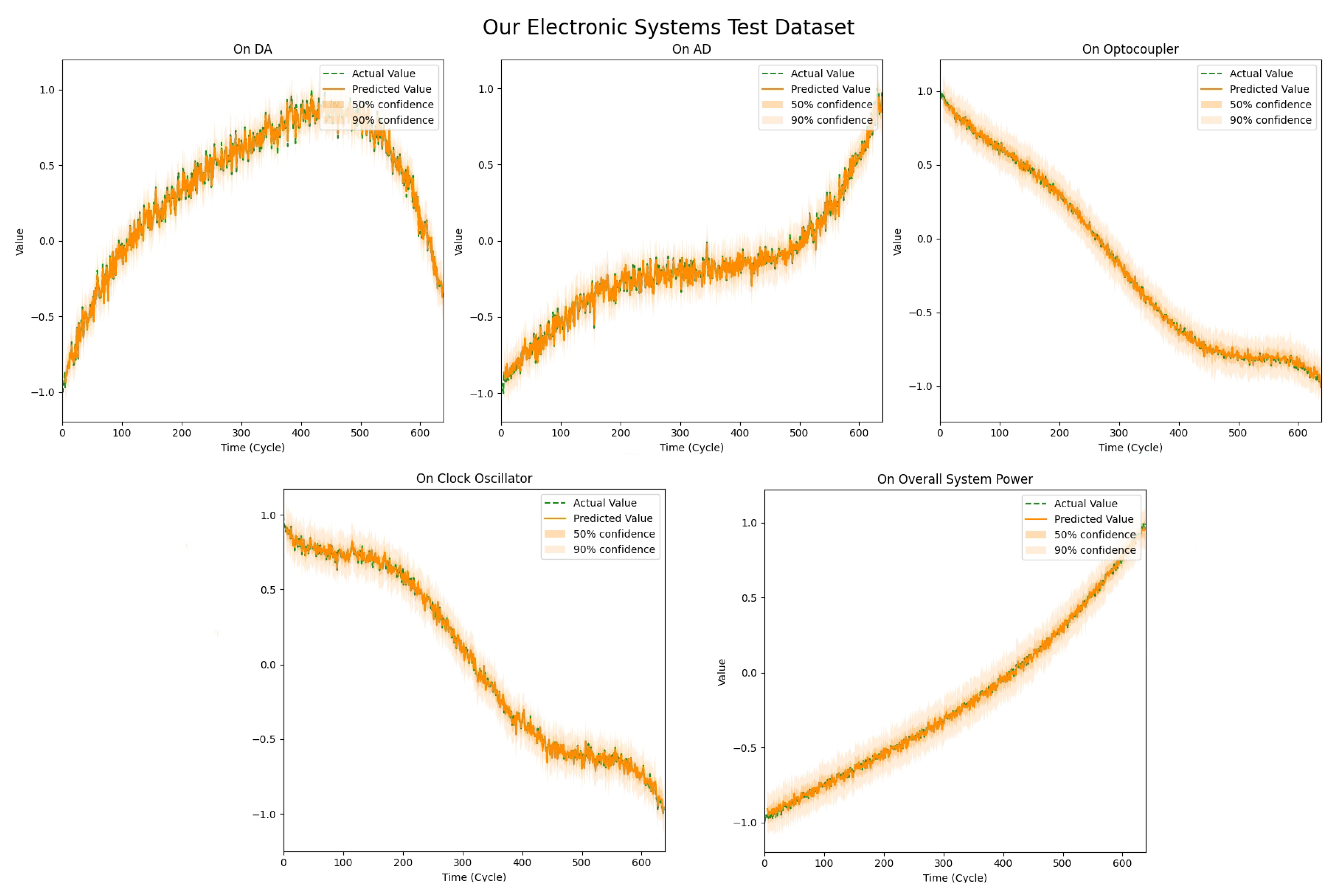
Our electronic systems: We visualized the prediction results of our electronic system test dataset, as shown in Figure 9. The figure compares the predicted and actual values, where the green dashed line represents the true values, the orange line indicates the predicted mean, and the orange shading denotes the prediction interval, reflecting the model’s uncertainty in its predictions.

The results show a high degree of consistency between the predicted and actual observed values, suggesting that the prediction model effectively captures the system’s behavior in most cases. Specifically, the prediction of overall system power is relatively stable, with the predicted values closely following the actual values, and the narrow prediction interval indicates high confidence in the model’s accuracy. For other features, such as the optocoupler and the clock oscillator, although the predicted values align with the actual values in terms of trends, there is higher uncertainty due to greater fluctuations, as indicated by the wider prediction intervals.

In summary, the prediction model demonstrates a good performance across different feature sequences, particularly for overall system power, DA, and AD. While some features, such as the optocoupler and the clock oscillator, show higher uncertainty in their predictions, the model still effectively captures the main trends in these system characteristics, providing valuable insights for further optimization of the system performance.

5. Conclusions

This paper proposes a multivariate time series forecasting framework, aiming to develop a concise, efficient, and high-performing predictive model. Unlike traditional complex multi-module designs, the proposed method enhances the extraction and modeling of multivariate features by integrating a decomposition-aware layer, which effectively separates and fuses global trends and local variations, and the temporal attention module. This design achieves a favorable balance between accuracy and computational efficiency. Furthermore, the framework incorporates probabilistic distribution forecasting based on likelihood functions, effectively addressing the challenges of dynamic variations and uncertainty. Extensive experiments on multiple real-world datasets demonstrate that the proposed method significantly outperforms the existing benchmark approaches in its predictive accuracy. Additionally, it exhibits strong robustness and flexibility across diverse application scenarios.