Stability Analysis of Batch Offline Action-Dependent Heuristic Dynamic Programming Using Deep Neural Networks

Abstract

In this paper, the theoretical stability of batch offline action-dependent heuristic dynamic programming (BOADHDP) is analyzed for deep neural network (NN) approximators for both the action value function and controller which are iteratively improved using collected experiences from the environment. Our findings extend previous research on the stability of online adaptive ADHDP learning with single-hidden-layer NNs by addressing the case of deep neural networks with an arbitrary number of hidden layers, updated offline using batched gradient descend updates. Specifically, our work shows that the learning process of the action value function and controller under BOADHDP is uniformly ultimately bounded (UUB), contingent on certain conditions related to NN learning rates. The developed theory demonstrates an inverse relationship between the number of hidden layers and the learning rate magnitude. We present a practical implementation involving a twin rotor aerodynamical system to emphasize the impact difference between the usage of single-hidden-layer and multiple-hidden-layer NN architectures in BOADHDP learning settings. The validation case study shows that BOADHDP with multiple hidden layer NN architecture implementation obtains $0.0034$ on the control benchmark, while the single-hidden-layer NN architectures obtain $0.0049$, outperforming the former by 1.58% by using the same collected dataset and learning conditions. Also, BOADHDP is compared with online adaptive ADHDP, proving the superiority of the former over the latter, both in terms of controller performance and data efficiency.

1. Introduction

Adaptive dynamic programming (ADP) has emerged as a powerful methodology for tuning control systems in modern applications, where complexity, nonlinearity, and uncertainty are commonplace. Originating from Werbos’ pioneering work [1], which was based on the seminal work on dynamic programming conducted by Bellman [2], ADP soon became a notable stream of research, with multiple ADP designs developed. Among the ADP designs, two distinct classes of solutions have emerged: heuristic dynamic programming (HDP) and dual heuristic programming (DHP) [3]. In the HDP framework, reinforcement learning is employed to determine the cost-to-go from the current state. The HDP convergence for the general nonlinear systems is presented in [4]. Conversely, in DHP, neural networks are used to learn the derivative of the cost function relative to the states, known as the costate vector [5]. The DHP convergence for linear systems was established in [6]. For both of those two classes of algorithms, there exists the action-dependent (AD) adaptation [7]. ADP has also addressed the class of discrete-time control problems [8,9,10,11,12,13] and continuous time systems [14,15,16].

Apart from the theoretical contributions, ADP designs have been validated on a wide array of real applications. In [17], ADP is applied to a helicopter tracking and trimming control task. In [18], neural network controllers tuned with the ADHDP method are applied to an engine torque and exhaust air–fuel ratio control for an automotive engine. A practical implementation in the context of an electric water heater is presented in [19], where the collected sensor data were used to learn in a model-free manner the Q-function and the controller.

Convergence and stability proofs of the iterative processes involved in ADP-like techniques have also been developed. In [6], the adaptive critic method is described, where two networks approximate the controller and the Lagrangian multipliers associated with the optimal control, respectively. The convergence of the interleaved successive update of the two networks has been analyzed. In [20], an online generalized ADP is issued for a system with input constraints. Then, using a Lyapunov approach, a uniformly ultimate boundedness (UUB) stability is proved. The convergence of the value-iteration HDP is established for the nonlinear discrete-time systems in [4]. In paper [21], the authors derive the UUB stability for direct HDP algorithms, proving that the actor and critic weights remain bounded. The actor and critic were approximated by a multilayer perceptron (MLP) with three layers: input, hidden, and output. However, the updated weights were only the ones from the hidden and output layers, like in a linear basis function approach. To overcome the practical limitations imposed by linear basis-function-type approximators, such as scalability and overfitting, the authors from paper [22] extended the stability analysis from [21] to MLPs to update both the input-to-hidden-layer weights and the hidden-to-output weights.

Current research in the field of reinforcement learning (RL), which studies the class of stochastic systems and controllers, shows significant performances when using deep NNs for control applications for both discretized systems [23] and continuous control tasks [24]. The advantage of deep neural networks over single-layer networks lies in their increased approximation capacity, which is achieved through multiple hidden layers. These layers enable the composition of features at different abstraction levels, creating a robust hierarchical representation. This hierarchical structure allows deep networks to learn and model complex nonlinear relationships within data more effectively than shallow networks. Thus, using multilayer NNs in ADP applications can enhance learning convergence and the overall controller performance. Also, using batch learning methods, which update the NN weights using collected past experiences simultaneously, is more data efficient compared to the single-transition learning, where the weights are updated one transition at a time. This also breaks the temporal correlations, helping NNs better generalize across a system’s state space. Typically, batch learning is combined with offline learning, where the weights are updated exclusively using a fixed dataset of transitions, without any adaptation during the controller’s runtime. Methods such as those in [19,24,25,26] demonstrate the benefits of using batch learning through a technique known as experience replay. In contrast, ref. [27] highlights an approach where the entire dataset of collected transitions is used for learning, in an offline manner.

This paper makes two key contributions. First, we provide a novel theoretical stability of ADHDP when utilizing deep neural networks as function approximators for both the action value function and the controller and for when batch learning is issued on the entire dataset of collected transitions from the system. This stands as an improvement over the stability analyses performed in [21,22], which were based on single-hidden-layer NN architectures updated online, with each transition collected during the system runtime. To this end, we prove that the batched offline ADHDP (BOADHDP) learning process is uniformly ultimately bounded (UUB) by using the Lyapunov stability approach. We show that the stability of the learning process is dependent on some conditions imposed on the NN learning rates and that these conditions also provide a relationship between the learning rate magnitudes and the number of hidden layers in the networks. Second, we issue a validation study on a twin rotor aerodynamical system (TRAS) to emphasize the superiority of employing multiple hidden layers in the NN approximators in the BOADHDP learning process. We also issue some comparison between BOADHDP and the online adaptive ADHDP algorithms from [21,22].

The rest of the paper is organized as follows. Section 2 describes the theoretical underpinnings of BOADHDP. Section 3 presents the multilayer neural network approximation of the action value function and controller. Section 4 provides the main theoretical results for the stability of BOADHDP. Section 5 illustrates the TRAS validation case study. Finally, the discussion and concluding remarks are presented in Section 6.

2. Problem Formulation

Let the discrete-time nonlinear system described by the state equation be

$${\mathit{x}}_{k+1}=F({\mathit{x}}_k,{\mathit{u}}_k),$$

(1)

where $k\in \mathbb{N}$ denotes the time index, ${\mathit{x}}_k={\left[x_{1,k},\dots ,x_{n,k}\right]}^T\in {\mathsf{\Omega }}_X\subset {\mathfrak{R}}^n$ the system state, ${\mathit{u}}_k={\left[u_{1,k},\dots ,u_{m,k}\right]}^T\in {\mathsf{\Omega }}_U\subset {\mathfrak{R}}^m$ the control input, $F:{\mathsf{\Omega }}_X\times {\mathsf{\Omega }}_U\to {\mathsf{\Omega }}_X$ the unknown continuously differentiable system function, and ${\mathsf{\Omega }}_X$ and ${\mathsf{\Omega }}_U$ the compact subsets of ${\mathfrak{R}}^n$ and ${\mathfrak{R}}^m$, respectively. The control input is generated by ${\mathit{u}}_k=C\left({\mathit{x}}_k\right)$, with $C:{\mathsf{\Omega }}_X\to {\mathsf{\Omega }}_U$ a time-invariant, continuous state feedback controller function with respect to the state $\mathit{x}$. For convention, vectors with ${\left[x_{1,k},\dots ,x_{n,k}\right]}^T$ are column vectors, while the ones without the transposition are row vectors.

For the optimal control problem, the objective is to find the optimal controller that minimizes the infinite value function, defined as follows:

$$V\left({\mathit{x}}_k\right)={\sum }_{i=k}^{\infty }r({\mathit{x}}_i, C({\mathit{x}}_i\left)\right) =r\left({\mathit{x}}_k, C\left({\mathit{x}}_k\right)\right)+V\left({\mathit{x}}_{k+1}\right),$$

(2)

where function $r:{\mathsf{\Omega }}_X\times {\mathsf{\Omega }}_U\to \mathfrak{R}$, having $r\left({\mathit{x}}_k,{\mathit{u}}_k\right)\ge 0, r\left(\mathrm{0,0}\right)=0$, is known as the penalty function, defined as $r\left({\mathit{x}}_k,{\mathit{u}}_k\right)=\mathsf{\Theta }\left({\mathit{x}}_k\right)+C{\left({\mathit{x}}_k\right)}^T\mathit{R}C\left({\mathit{x}}_k\right)$, where $\mathsf{\Theta }:{\mathsf{\Omega }}_X\to \mathfrak{R}$ is the penalty term describing the system’s desired behavior as a positive semidefinite function, and $\mathit{R}\in {\mathfrak{R}}^{m\times m}$ is a square positive definite command weighting matrix, as in [4]. The optimal value function [1] is defined as

$$V^{*}\left({\mathit{x}}_k\right)=\underset{C\left({\mathit{x}}_k\right)}{\min }\left\{r\left({\mathit{x}}_k, C\left({\mathit{x}}_k\right)\right)+V^{*}\left({\mathit{x}}_{k+1}\right)\right\}.$$

(3)

The optimal controller is found by applying the argmin() operator to Equation (3), as

$$C^{*}\left({\mathit{x}}_k\right)=\mathit{arg}\underset{C\left({\mathit{x}}_k\right)}{\min }\left\{r\left({\mathit{x}}_k, C\left({\mathit{x}}_k\right)\right)+V^{*}\left({\mathit{x}}_{k+1}\right)\right\}.$$

(4)

With the system function $F$ unknown, one cannot apply the well-known ADP methods for the system (1) directly in order to arrive at (3) and (4). Therefore, the introduction of action value functions is mandatory to handle the model-free case.

The action value function proposed by [28] evaluates both the current state and the command. It is defined as

$$Q\left({\mathit{x}}_k,{\mathit{u}}_k\right)=r\left({\mathit{x}}_k,{\mathit{u}}_k\right)+V\left({\mathit{x}}_{k+1}\right).$$

(5)

Compared to the value function (2), the action value function represents the cost of issuing a command ${\mathit{u}}_k$ in a state ${\mathit{x}}_k$, plus the value function of the next state ${\mathit{x}}_{k+1}$. Mainly, Equation (5) evaluates all possible actions ${\mathit{u}}_k\in {\mathsf{\Omega }}_U$ followed by the controller $C\left({\mathit{x}}_{k+1}\right)$. Equation (5) can also be written, according to [28], as

$$Q\left({\mathit{x}}_k,{\mathit{u}}_k\right)=r\left({\mathit{x}}_k,{\mathit{u}}_k\right)+Q\left({\mathit{x}}_{k+1},C\left({\mathit{x}}_{k+1}\right)\right).$$

(6)

From [28], similarly to the value function (3), the optimal action value function is defined as

$$Q^{*}\left({\mathit{x}}_k\right)=\underset{C\left({\mathit{x}}_k\right)}{\min }\left\{r\left({\mathit{x}}_k,{\mathit{u}}_k\right)+Q^{*}\left({\mathit{x}}_{k+1},C\left({\mathit{x}}_{k+1}\right)\right)\right\},$$

(7)

and the optimal controller is represented by

$$C^{*}\left({\mathit{x}}_k\right)=\mathit{arg}\underset{C\left({\mathit{x}}_k\right)}{\min }\left\{r\left({\mathit{x}}_k,{\mathit{u}}_k\right)+Q^{*}\left({\mathit{x}}_{k+1},C\left({\mathit{x}}_{k+1}\right)\right)\right\}.$$

(8)

ADHDP Algorithm

Arriving at the optimal action value function and controller requires an iterative procedure consisting of $j$ steps, where the action value function and controller are continuously updated, according to [28]. Starting with an initial controller $C_0\left({\mathit{x}}_k\right)$ and an action value function, e.g., $Q_0\left({\mathit{x}}_k,{\mathit{u}}_k\right)=0$, the action value function evaluation is issued by

$$Q_1\left({\mathit{x}}_k,{\mathit{u}}_k\right)=r\left({\mathit{x}}_k,{\mathit{u}}_k\right)+Q_0\left({\mathit{x}}_{k+1},C_0\left({\mathit{x}}_{k+1}\right)\right).$$

(9)

Then, the controller is updated using

$$C_1\left({\mathit{x}}_k\right)=\mathit{arg}\underset{C\left({\mathit{x}}_k\right)}{\min }\left\{r\left({\mathit{x}}_k,{\mathit{u}}_k\right)+Q_0\left({\mathit{x}}_{k+1},C\left({\mathit{x}}_{k+1}\right)\right)\right\}.$$

(10)

At the $j^{th}$ iteration, the action value function update is

$$Q_{j+1}\left({\mathit{x}}_k,{\mathit{u}}_k\right)=r\left({\mathit{x}}_k,{\mathit{u}}_k\right)+Q_j\left({\mathit{x}}_{k+1},C_j\left({\mathit{x}}_{k+1}\right)\right),$$

(11)

while the controller update law is

$$C_{j+1}\left({\mathit{x}}_k\right)=\mathit{arg}\underset{C\left({\mathit{x}}_k\right)}{\min }\left\{r\left({\mathit{x}}_k,{\mathit{u}}_k\right)+Q_j\left({\mathit{x}}_{k+1},C\left({\mathit{x}}_{k+1}\right)\right)\right\}.$$

(12)

The iteration scheme consisting of the repetitive application of Equations (11) and (12) runs as $j\to \infty$.

Remark 1.

A policy iteration algorithm requires an initially known stabilizing controller $C_0\left({\mathit{x}}_k\right)$, whereas, for value iteration schemes, this need is avoided.

In the next section, the implementation of the controller and action value function update is issued using a neural network function approximation for $Q_j\left({\mathit{x}}_k,{\mathit{u}}_k\right)$ and $C_j\left({\mathit{x}}_k\right)$.

3. Neural Network Implementation for BOADHDP

The recurrent ADP scheme described by Equations (11) and (12) is practically implemented using function approximators for the action value function and controller. To this end, neural networks (NNs) are used, due to their universal function approximation property, which is able to handle multidimensional nonlinear systems (1). The tuning of the NN weights from each individual layer requires both input–output training data and the employment of the backpropagation mechanism, which can be best described as a gradient-based update rule.

The training data for the controller and action value function are collected from the controlled system (1) and take the form of transition tuples ${(\mathit{x}}_k, {\mathit{u}}_k,r\left({\mathit{x}}_k,{\mathit{u}}_k\right), {\mathit{x}}_{k+1})$ stored in a dataset $D_M=\{{(\mathit{x}}_k, {\mathit{u}}_k,r\left({\mathit{x}}_k,{\mathit{u}}_k\right), {\mathit{x}}_{k+1})\}$, with $k=1:M$. The main objective of the data collection phase is to uniformly sample the state space ${\mathsf{\Omega }}_X\times {\mathsf{\Omega }}_U$, sufficiently exploring the systems’ dynamics.

The action value function and controller NN weight tuning algorithm, using a gradient descent, is described in Section 3.1 and Section 3.2. The weight gradient update uses the entirety of the collected transitions from $D_M$, compared to the methods from [21,22] which use only one transition per gradient update. This method is called batch optimization, and its utilization is a common practice for the application of RL and ADP applied to complex nonlinear systems.

For the batch learning implementation, the action value function and controller update is made simultaneously for the entire dataset $D_M$. Therefore, let ${\mathbf{X}}_p=\left[{\mathit{x}}_1,\dots ,{\mathit{x}}_{M-1}\right]$, ${\mathbf{X}}_f=\left[{\mathit{x}}_2,\dots ,{\mathit{x}}_M\right]$ of size $n\times (M-1)$, and $\mathsf{{\rm Y}}=\left[{\mathit{u}}_1,\dots ,{\mathit{u}}_{M-1}\right]$ of size $m\times (M-1)$ be vectors that lump all states and commands collected in the dataset $D_M$. Also, let $\mathsf{\Xi }=\left[\begin{array}{c}{\mathbf{X}}_p\\ \mathsf{{\rm Y}}\end{array}\right]$ be the matrix of the concatenation of the states and command matrices converted into a matrix resembling the action value function input.

Stating ${\tilde{Q}}_j\left({\mathit{x}}_k, {\mathit{u}}_k,{\mathit{W}}_Q\right)$ and ${\tilde{C}}_j\left({\mathit{x}}_k,{\mathit{W}}_C\right)$ as the action value function and controller functions, respectively, approximated by NNs, and with ${\widehat{\mathit{W}}}_Q$ and ${\widehat{\mathit{W}}}_C$ representing the entirety of the action value function and controller weights, respectively, the gradient descend update is next detailed.

3.1. Action Value Function NN Approximation

The action value function NN has the scope of approximating (11). Having as inputs the state ${\mathit{x}}_k$ and ${\mathit{u}}_k$, the state action function NN is described as

$$Q_j\left({\mathbf{X}}_p, \mathsf{{\rm Y}},{\mathit{W}}_Q\right)=Q\left({\mathbf{X}}_p, \mathsf{{\rm Y}},{\mathit{W}}_Q^j\right)={\mathit{z}}_Q^{L_Q}={\mathit{W}}_{Q,j}^{L_Q}{\mathit{\kappa }}_Q^{L_Q-1},$$

(13)

where

$${\mathit{z}}_Q^{l_Q}={\mathit{W}}_{Q,j}^{l_Q}{\mathit{\kappa }}_Q^{l_Q-1},\mathrm{for} l_Q=1,\dots ,L_Q,$$

$${\mathit{\kappa }}_Q^{l_Q}=\varphi \left({\mathit{z}}_Q^{l_Q}\right),$$

and $L_Q$ is the total number of layers, ${\mathit{W}}_{Q,j}^l\in {\mathfrak{R}}^{h_Q^{l_Q}\times h_Q^{l_Q-1}}$ is the ideal hidden-layer weight matrix from the iteration j and layer $l_Q$, and $h_Q^{l_Q}$ is the number of neurons from layer $l_Q$. The size of $Q\left({\mathbf{X}}_p, \mathsf{{\rm Y}},{\mathit{W}}_Q^j\right)$ is $1\times M$. Here, $\varphi \left(·\right)=\mathrm{t}\mathrm{a}\mathrm{n}\mathrm{h}(·)$ represents the activation function and can take any form, such as $\mathrm{t}\mathrm{a}\mathrm{n}\mathrm{h}(·)$, $\mathrm{R}\mathrm{e}\mathrm{L}\mathrm{u}(·)$, $\mathrm{s}\mathrm{i}\mathrm{g}\mathrm{m}\mathrm{o}\mathrm{i}\mathrm{d}(·)$, and so on. The vector ${\mathit{\kappa }}^l$ is the $l_Q$ layer activation output. For the first layer, we have ${\mathit{\kappa }}_Q^0=\mathsf{\Xi }$.

Generally, weights ${{\mathit{W}}_{Q,j}^{l_Q}}^T$, for $l_Q=0,\dots , L_Q$ are generally unknown due to the existing approximation errors in the weight update backpropagation rule. Hence, working with the real action value function $Q_j\left({\mathbf{X}}_p, \mathsf{{\rm Y}},{\mathit{W}}_Q\right)$ is not realistic, but only with some approximations of it. Noting with ${\widehat{\mathit{W}}}_{Q,j}$ the entirety of the action value function weights, the output of the approximate action value function NN has the form of

$${\widehat{Q}}_j\left({\mathbf{X}}_p, \mathsf{{\rm Y}},{\widehat{\mathit{W}}}_Q\right)=\widehat{Q}\left({\mathbf{X}}_p, \mathsf{{\rm Y}},{\widehat{\mathit{W}}}_Q^j\right)={\widehat{\mathit{z}}}_Q^{L_Q}={\widehat{\mathit{W}}}_{Q,j}^{L_Q}{\widehat{\mathit{\kappa }}}_Q^{L_Q-1},$$

(14)

where

$${\mathit{z}}_Q^{l_Q}={\mathit{W}}_{Q,j}^{l_Q}{\mathit{\kappa }}_Q^{l_Q-1}, \mathrm{for} l_Q=1,\dots ,L_Q,$$

$${\mathit{\kappa }}_Q^{l_Q}=\varphi \left({\mathit{z}}_Q^{l_Q}\right),$$

and where ${\widehat{\mathit{W}}}_{Q,j}^l\in {\mathfrak{R}}^{h_Q^{l_Q}\times h_Q^{l_Q-1}}$ represents an estimation of the ideal weights for $l_Q=0,\dots , L_Q$. To update the action value function NN weights, an internal gradient update loop is issued for the $i_Q=0,\dots ,{\mathsf{{\rm I}}}_Q$ steps, having the weights initialized with ${\widehat{\mathit{W}}}_{Q,j,0}={\widehat{\mathit{W}}}_{Q,j}$. At each iteration $i$, the following optimization problem needs to be solved,

$${\widehat{\mathit{W}}}_{Q,j,i_Q+1}=\underset{\widehat{\mathit{W}}}{\mathrm{a}\mathrm{r}\mathrm{g}\mathrm{m}\mathrm{i}\mathrm{n}}{\displaystyle \frac{1}{M}}{\mathit{E}}_{Q,j,i_Q},$$

(15)

where

$${\mathit{E}}_{Q,j,i_Q}={{{\mathit{e}}_{Q,j,i_Q}\mathit{e}}_{Q,j,i_Q}}^T$$

(16)

and

$${\mathit{e}}_{Q,j,i_Q}={\left(\widehat{Q}\left({\mathbf{X}}_p, \mathsf{{\rm Y}},\widehat{\mathit{W}}\right)-{\mathit{\eta }}_{Q,j,i_Q}\right)}^T,$$

(17)

having ${\mathit{\eta }}_{Q,j,i_Q}=r\left({\mathbf{X}}_p,\mathsf{{\rm Y}}\right)-\gamma \widehat{Q}\left({\mathbf{X}}_f,\tilde{C}\left({\mathbf{X}}_f,{\widehat{\mathit{W}}}_{C,j}\right),{\widehat{\mathit{W}}}_{Q,j,i_Q}\right)$.

Here, ${\mathit{e}}_{Q,j,i_Q}$ represents the prediction error in the form of a TD error. The state action function weights are updated by the rule

$${\widehat{\mathit{W}}}_{Q,j, i_Q+1}^{l_Q}={\widehat{\mathit{W}}}_{Q,j, i_Q}^{l_Q}-{\alpha }_Q{\displaystyle \frac{\partial {\mathit{E}}_{Q,j,i_Q}}{\partial {\widehat{\mathit{W}}}_{Q,j, i_Q}^{l_Q}}},$$

(18)

where ${\alpha }_Q>0$ is the action value function NN learning rate and

$${\displaystyle \frac{\partial {\mathit{E}}_{Q,j,i_Q}}{\partial {\widehat{\mathit{W}}}_{Q,j, i_Q}^{l_Q}}}={\displaystyle \frac{\partial {\mathit{E}}_{Q,j,i_Q}}{\partial {\widehat{\mathit{z}}}_Q^{l_Q}}}{\displaystyle \frac{\partial {\widehat{\mathit{z}}}_Q^{l_Q}}{\partial {\widehat{\mathit{W}}}_{Q,j, i_Q}^{l_Q}}}={\displaystyle \frac{\partial {\mathit{E}}_{Q,j,i_Q}}{\partial {\widehat{\mathit{z}}}_Q^{l_Q}}}{{\widehat{\mathit{\kappa }}}_Q^{l_Q-1}}^T$$

(19)

$${\displaystyle \frac{\partial {\mathit{E}}_{Q,j,i_Q}}{\partial {\widehat{\mathit{z}}}_Q^{l_Q}}}={\displaystyle \frac{\partial {\mathit{E}}_{Q,j,i_Q}}{\partial {\widehat{\mathit{z}}}_Q^{l_Q+1}}}{\displaystyle \frac{\partial {\widehat{\mathit{z}}}_Q^{l_Q+1}}{\partial {\mathit{\kappa }}_Q^{l_Q}}}{\displaystyle \frac{\partial {\mathit{\kappa }}_Q^{l_Q}}{\partial {\widehat{\mathit{z}}}_Q^{l_Q}}}={{\widehat{\mathit{W}}}_{Q,j, i_Q}^{l_Q+1}}^T{\displaystyle \frac{\partial {\mathit{E}}_{Q,j,i_Q}}{\partial {\widehat{\mathit{z}}}_Q^{l_Q+1}}}⨀\dot{\varphi }\left({\widehat{\mathit{z}}}_Q^{l_Q}\right)$$

(20)

The sign $⨀$ corresponds to the Hadamard product. Then, the weights ${\widehat{\mathit{W}}}_{Q,j+1}$ of $j+1$ are actualized as ${\widehat{\mathit{W}}}_{Q,j+1}={\widehat{\mathit{W}}}_{Q,j,{\mathsf{{\rm I}}}_{\mathrm{Q}}}$.

3.2. Controller NN Approximation

The controller NN has the scope of approximating $C\left({\mathit{x}}_k\right)$. Noting with ${\mathit{W}}_{C,j}$ the entirety of the controller weights, and having as input the state ${\mathbf{X}}_p$, the output is computed as

$$C_j\left({\mathbf{X}}_p,{\mathit{W}}_C\right)=C\left({\mathbf{X}}_p,{\mathit{W}}_{C,j}\right)={{\mathit{z}}_C}^{L_C}={\mathit{W}}_{C,j}^{L_C}{{\mathit{\kappa }}_C}^{L_C-1},$$

(21)

where

$${{\mathit{z}}_C}^{l_C}={\mathit{W}}_{C,j}^{l_C}{{\mathit{\kappa }}_C}^{l_C-1}, \mathrm{for} l_C=1,\dots ,L_C$$

$${{\mathit{\kappa }}_C}^{l_C}=\varphi \left({{\mathit{z}}_C}^{l_C}\right),$$

and where ${\mathit{W}}_{C,j}^{l_C}\in {\mathfrak{R}}^{h_Q^{l_C}\times h_Q^{l_C-1}}$ represents an estimation of the iteration j of the ideal weights for the $l_C=0,\dots , L_C$ layers. Noting with ${\widehat{\mathit{W}}}_{C,j}$ the estimation of the ideal weights, the output of the controller NN is

$${\widehat{C}}_j\left({\mathbf{X}}_p,{\widehat{\mathit{W}}}_C\right)=\widehat{C}\left({\mathbf{X}}_p,{\widehat{\mathit{W}}}_{C,j}\right)={{\widehat{\mathit{z}}}_C}^{L_C}={\widehat{\mathit{W}}}_{C,j}^{L_C}{{\widehat{\mathit{\kappa }}}_C}^{L_C-1}$$

(22)

with

$${{\widehat{\mathit{z}}}_C}^{l_C}={\widehat{\mathit{W}}}_{C,j}^{l_C}{{\widehat{\mathit{\kappa }}}_C}^{l_C-1}, \mathrm{for} l_C=1,\dots ,L_C$$

$${{\widehat{\mathit{\kappa }}}_C}^{l_C}=\varphi \left({{\widehat{\mathit{z}}}_C}^{l_C}\right)$$

and where ${\widehat{\mathit{W}}}_{C,j}^{l_C}$ represents an estimation of the real weights. To update the controller weights, one needs to issue an internal gradient update loop for the $i_C=0,\dots ,{\mathsf{{\rm I}}}_C$ steps, having the weights initialized with ${\widehat{\mathit{W}}}_{C,j,0}={\widehat{\mathit{W}}}_{C,j}$. At each iteration $i_C$, the following optimization problem needs to be minimized for the entirety of the collected dataset, as follows,

$${\widehat{\mathit{W}}}_{C,j,i_C}=\underset{\widehat{\mathit{W}}}{\mathrm{a}\mathrm{r}\mathrm{g}\mathrm{m}\mathrm{i}\mathrm{n}}{\displaystyle \frac{1}{M}}{\mathit{E}}_{C,j,i_C}$$

(23)

where

$${\mathit{E}}_{C,j,i_C}={{{\mathit{e}}_{C,j,i_C}\mathit{e}}_{C,j,i_C}}^T$$

(24)

and

$${\mathit{e}}_{C,j,i_C}=\widehat{Q}\left({\mathbf{X}}_p, \widehat{C}\left({\mathbf{X}}_p,\widehat{\mathit{W}}\right),{\widehat{\mathit{W}}}_{Q,j+1}\right)$$

(25)

where ${\alpha }_C>0$ represents the controller NN learning rate.

The update of each individual weights is

$${\widehat{\mathit{W}}}_{C,j, i_C+1}^{l_C}={\widehat{\mathit{W}}}_{C,j, i_C}^{l_C}-{\alpha }_C{\displaystyle \frac{\partial {\mathit{E}}_{C,j,i_C}}{\partial {\widehat{\mathit{W}}}_{C,j, i_C}^{l_C}}}$$

(26)

where

$${\displaystyle \frac{\partial {\mathit{E}}_{C,j,i_C}}{\partial {\widehat{\mathit{W}}}_{C,j, i_C}^{l_C}}}={\displaystyle \frac{\partial {\mathit{E}}_{C,j,i_C}}{\partial {\widehat{\mathit{z}}}_C^{l_C}}}{\displaystyle \frac{\partial {\widehat{\mathit{z}}}_C^{l_C}}{\partial {\widehat{\mathit{W}}}_{Q,j, i_C}^{l_C}}}={\displaystyle \frac{\partial {\mathit{E}}_{C,j,i_C}}{\partial {\widehat{\mathit{z}}}_C^{l_C}}}{{\widehat{\mathit{\kappa }}}_C^{l_C-1}}^T$$

(27)

$${\displaystyle \frac{\partial {\mathit{E}}_{C,j,i_C}}{\partial {\widehat{\mathit{z}}}_C^{l_C}}}={\displaystyle \frac{\partial {\mathit{E}}_{C,j,i_C}}{\partial {\widehat{\mathit{z}}}_C^{l_C+1}}}{\displaystyle \frac{\partial {\widehat{\mathit{z}}}_C^{l_C+1}}{\partial {\mathit{\kappa }}^{l_C}}}{\displaystyle \frac{\partial {\mathit{\kappa }}^{l_C}}{\partial {\widehat{\mathit{z}}}_C^{l_C}}}={{\widehat{\mathit{W}}}_{C,j, i_C}^{l_C+1}}^T{\displaystyle \frac{\partial {\mathit{E}}_{C,j,i_C}}{\partial {\widehat{\mathit{z}}}_C^{l_C+1}}}⨀\dot{\varphi }\left({\widehat{\mathit{z}}}_C^{l_C}\right).$$

(28)

To issue the update (28), it is necessary to compute the gradient of the action value function with respect to the controller output. This is computed as

$${\displaystyle \frac{\partial {\mathit{E}}_{C,j,i_C}}{\partial {\widehat{\mathit{z}}}_C^{L_C}}}={\displaystyle \frac{\partial {\mathit{E}}_{C,j,i_C}}{\partial \widehat{C}\left({\mathbf{X}}_p,{\widehat{\mathit{W}}}_{C,j,i_C}\right)}}={\displaystyle \frac{\partial {\mathit{E}}_{C,j,i_C}}{\partial {\widehat{\mathit{z}}}_Q^1}}{\displaystyle \frac{\partial {\widehat{\mathit{z}}}_Q^1}{\partial {{\widehat{\mathit{\kappa }}}_Q}^0}}{\displaystyle \frac{\partial {{\widehat{\mathit{\kappa }}}_Q}^0}{\partial \widehat{C}\left({\mathbf{X}}_p,{\widehat{\mathit{W}}}_{C,j,i_C}\right)}}={\mathsf{\Psi }}^{\mathrm{T}}\left({{\widehat{\mathit{W}}}_{C,j,i}^1}^T{\displaystyle \frac{\partial {\mathit{E}}_{C,j,i_C}}{\partial {\widehat{\mathit{z}}}_Q^1}}\right)={\mathsf{\Omega }}_{j,i}$$

(29)

where $\mathsf{\Psi }=\left[\begin{array}{c}{\mathbf{0}}_{n\times m}\\ {\mathit{I}}_m\end{array}\right]$ and ${\mathit{I}}_m$ are the identity matrix, of dimensions $m\times m$, and ${\mathbf{0}}_{n\times m}$, a $n\times m$ matrix of zeros. Then, the weights ${\widehat{\mathit{W}}}_{C,j+1}$ of $j+1$ are actualized as ${\widehat{\mathit{W}}}_{C,j+1}={\widehat{\mathit{W}}}_{C,j,{\mathsf{{\rm I}}}_C}$.

3.3. Batch Offline ADHDP with Multiple-Hidden-Layer NN Algorithm

Next, the BOADHDP algorithm using multiple-hidden-layer NN function approximators is detailed. The algorithm consists of consecutive steps where the action value and controller NNs are updated.

• Initialize ${\alpha }_Q$, ${\alpha }_C$, ${\mathsf{{\rm I}}}_{\mathrm{Q}}$, ${\mathsf{{\rm I}}}_{\mathrm{C}}$, ${\mathsf{\Delta }}_Q$. Initialize the NN architectures for ${\widehat{Q}}_j({\mathbf{X}}_p, \mathsf{{\rm Y}},{\widehat{\mathit{W}}}_Q)$ and ${\widehat{C}}_j({\mathbf{X}}_p,{\widehat{\mathit{W}}}_C)$ by setting $L_Q$, $L_C$, and their respective weights. Let $j=0$ and $i_Q=i_C=0$.
• Collect $M$ transitions from system (1) and construct the database $D_M$.
• At iteration $j$, set $i_Q=0$ and ${\widehat{\mathit{W}}}_{Q,j,i_Q}={\widehat{\mathit{W}}}_{Q,j}$. Then, update the weights from all $L_Q$ layers using (18) for $i_Q={\overline{0,\mathsf{{\rm I}}}}_Q$. Finally, set ${\widehat{\mathit{W}}}_{Q,j+1}={\widehat{\mathit{W}}}_{Q,j,{\mathsf{{\rm I}}}_{\mathrm{Q}}}$.
• Set $i_C=0$ and ${\widehat{\mathit{W}}}_{C,j,i_C}={\widehat{\mathit{W}}}_{C,j}$. Then, update the weights from all $L_C$ layers using (26) for $i_C={\overline{0,\mathsf{{\rm I}}}}_C$. Finally, set ${\widehat{\mathit{W}}}_{C,j+1}={\widehat{\mathit{W}}}_{C,j,{\mathsf{{\rm I}}}_{\mathrm{C}}}$.
• If the condition $‖{\widehat{\mathit{W}}}_{Q,j}-{\widehat{\mathit{W}}}_{Q,j-1}‖<{\mathsf{\Delta }}_Q$ is not met, update $j=j+1$ and go to Step 3. Else, stop the iterative algorithm.

4. UUB Convergence

In this section, the convergence of the NN weights to a fixed point is examined. By using a Lyapunov function, the stability of the weight evolution to the fixed point is proved to be UUB under some specific conditions.

4.1. Lyapunov Approach Description

Each iteration $j$ of the BOADHDP algorithm consists of a total cumulated number of $\mathsf{{\rm I}}={\mathsf{{\rm I}}}_Q+{\mathsf{{\rm I}}}_C$ gradient steps for both action value function and controller. Let a new iteration index be defined as $i=1:j\ast \mathsf{{\rm I}}$, namely $i\in [1,\dots ,{\mathsf{{\rm I}}}_Q,{\mathsf{{\rm I}}}_Q+1,\dots , \mathsf{{\rm I}},\mathsf{{\rm I}}+1,\dots ,\mathsf{{\rm I}}+{\mathsf{{\rm I}}}_Q,\mathsf{{\rm I}}+{\mathsf{{\rm I}}}_Q+1,\dots , 2\mathsf{{\rm I}},\dots ]$, which represents a fine-grained iteration over both gradient action value function and controller. During $i\in [j\mathsf{{\rm I}},\mathrm{j}\mathsf{{\rm I}}+{\mathsf{{\rm I}}}_Q]$, only the action value function neural network weights ${\widehat{\mathit{W}}}_{Q,j,i}$ are updated using (18), while ${\widehat{\mathit{W}}}_{C,j,i}$ remains unchanged. On the other side, for $i\in [j\mathsf{{\rm I}}+{\mathsf{{\rm I}}}_Q,\mathrm{j}\mathsf{{\rm I}}+{\mathsf{{\rm I}}}_Q+{\mathsf{{\rm I}}}_C]$, only the controller weights ${\widehat{\mathit{W}}}_{C,j,i}$ are updated using (26), while the action value function weights ${\widehat{\mathit{W}}}_{Q,j,i}$ remain unchanged. To simplify the notation, we substitute ${\widehat{\mathit{W}}}_{Q,j,i}$ and ${\widehat{\mathit{W}}}_{C,j,i}$ with ${\widehat{\mathit{W}}}_{Q,i}$ and ${\widehat{\mathit{W}}}_{C,i}$, respectively.

Let ${\mathit{W}}_Q^{*}$ and ${\mathit{W}}_C^{*}$ represent the optimal weights of the action value function NN and the controller NN, and let the weight estimation errors between the approximation of the real weights and the optimal ones be ${\overline{\mathit{W}}}_{Q,i}={\widehat{\mathit{W}}}_{Q,i}-{\mathit{W}}_Q^{*}$, ${\overline{\mathit{W}}}_{C,i}={\widehat{\mathit{W}}}_{C,i}-{\mathit{W}}_C^{*}$.

Therefore, the difference between the estimated weights and the optimal ones at each layer of both the action value function and the controller NN at each iteration $i$ is, according to (18) and (26),

$${\overline{\mathit{W}}}_{Q,i+1}^{l_Q}={\widehat{\mathit{W}}}_{Q,i+1}^{l_Q}-{\mathit{W}}_Q^{l_Q,*}={\widehat{\mathit{W}}}_{Q,i}^{l_Q}-{\alpha }_Q{\displaystyle \frac{\partial {\mathit{E}}_{Q,i}}{\partial {\widehat{\mathit{W}}}_{Q,i}^{l_Q}}}-{\mathit{W}}_Q^{l_Q,*}={\overline{\mathit{W}}}_{Q,i}^{l_Q}-{\alpha }_Q{\displaystyle \frac{\partial {\mathit{E}}_{Q,i}}{\partial {\widehat{\mathit{W}}}_{Q,i}^{l_Q}}}$$

(30)

$${\overline{\mathit{W}}}_{C,i+1}^{l_C}={\widehat{\mathit{W}}}_{C,i+1}^{l_C}-{\mathit{W}}_C^{l_C,*}={\widehat{\mathit{W}}}_{C,i}^{l_C}-{\alpha }_C{\displaystyle \frac{\partial {\mathit{E}}_{C,i}}{\partial {\widehat{\mathit{W}}}_{C,i}^{l_C}}}-{\mathit{W}}_C^{l_C,*}={\overline{\mathit{W}}}_{C,i}^{l_C}-{\alpha }_C{\displaystyle \frac{\partial {\mathit{E}}_{C,i}}{\partial {\widehat{\mathit{W}}}_{C,i}^{l_C}}}.$$

(31)

Then, based on (14), (18), (22), and (29), define the following dynamical system with the nonlinear difference equation system, where $P$ represents a nonlinear function,

$$\begin{gathered} \left\{\left[\begin{array}{c}{\overline{\mathit{W}}}_{Q,i+1}\\ {\overline{\mathit{W}}}_{C,i+1}\end{array}\right]=\right.\left[\begin{array}{c}{\overline{\mathit{W}}}_{Q,i}\\ {\overline{\mathit{W}}}_{C,i}\end{array}\right]- \\ P\left(\begin{array}{c}{\widehat{\mathit{W}}}_{Q,i},{\widehat{\mathit{W}}}_{Q,i-1},\varphi \left({\widehat{\mathit{W}}}_{Q,i}^1\mathsf{\Xi }\right),\varphi \left({\widehat{\mathit{W}}}_{Q,i-1}^1\mathsf{\Xi }\right),\dots ,\varphi \left({\widehat{\mathit{W}}}_{Q,i}^{L_Q}{{\widehat{\mathit{\kappa }}}_Q}^{L_Q-1}\right),\varphi \left({\widehat{\mathit{W}}}_{Q,i-1}^{L_Q}{{\widehat{\mathit{\kappa }}}_Q}^{L_Q-1}\right)\\ {\widehat{\mathit{W}}}_{C,i},{\widehat{\mathit{W}}}_{C,i},\varphi \left({\widehat{\mathit{W}}}_{C,i}^1{\mathbf{X}}_p\right),\varphi \left({\widehat{\mathit{W}}}_{C,i-1}^1{\mathbf{X}}_p\right),\dots ,\varphi \left({\widehat{\mathit{W}}}_{C,i}^{L_C}{{\widehat{\mathit{\kappa }}}_C}^{L_C-1}\right),\varphi \left({\widehat{\mathit{W}}}_{C,i-1}^{L_C}{{\widehat{\mathit{\kappa }}}_C}^{L_C-1}\right)\end{array}\right). \end{gathered}$$

(32)

Definition 1.

The equilibrium point of a system (32) is said to be uniformly ultimately bounded (UUB) with bound $\chi >0$ if, for any $\psi >0$ and $i_0>0$, there exists a positive number $N=N(\psi ,\chi )$ independent of $i_0$, such that $‖\begin{array}{c}{\overline{\mathit{W}}}_{Q,i}\\ {\overline{\mathit{W}}}_{C,i}\end{array}‖\le \chi$ for all $i\ge N+i_0$ when $‖\begin{array}{c}{\overline{\mathit{W}}}_{Q,i_0}\\ {\overline{\mathit{W}}}_{C,i_0}\end{array}‖\le \psi$.

4.2. Preliminary Results

In the following, the UUB property of the system (32) is demonstrated for the update rules (18) and (26), both of which make the weights of the two approximating NNs enter a region with the center in the optimal weights ${\mathit{W}}_Q^{*}$ and ${\mathit{W}}_C^{*}$. Some fundamental assumptions are next introduced.

Assumption 1.

The optimal NN weights for the action value function and the controller and the activation function $\varphi (·)$ are bounded by positive constants, i.e., $‖W_Q^{*}‖\le W_{Q,max}^{*}$, $‖W_C^{*}‖\le W_{C,max}^{*}$, $‖\varphi \left(·\right)‖\le {\varphi }_{max}$.

Lemma 1.

Under Assumption 1, it is implied that the first difference of ${\Gamma }_{Q,i}^{L_Q}={\displaystyle \frac{1}{{\alpha }_Q}}tr\left\{{{\overline{\mathit{W}}}_{Q,i}^{L_Q}}^T{\overline{\mathit{W}}}_{Q,i}^{L_Q}\right\}$ is given by

$$\mathsf{\Delta }{\mathsf{\Gamma }}_{Q,i}^{L_Q}=-tr\left\{2{\overline{\mathit{W}}}_{Q,i}^{L_Q}\varphi \left({\widehat{\mathit{z}}}_Q^{L_Q-1}\right){{\mathit{e}}_{Q,i}}^T\right\}+{\alpha }_{Q}tr\left\{{\mathit{e}}_{Q,i}\varphi {\left({\widehat{\mathit{z}}}_Q^{L_Q-1}\right)}^T\varphi \left({\widehat{\mathit{z}}}_Q^{L_Q-1}\right){{\mathit{e}}_{Q,i}}^T\right\}.$$

(33)

Proof. 

Let $\mathsf{\Delta }{\mathsf{\Gamma }}_{Q,i}^{L_Q}$ be described as

$$\mathsf{\Delta }{\mathsf{\Gamma }}_{Q,i}^{L_Q}={\displaystyle \frac{1}{{\alpha }_Q}}tr\left\{{{\overline{\mathit{W}}}_{Q,i+1}^{L_Q}}^T{\overline{\mathit{W}}}_{Q,i+1}^{L_Q}-{{\overline{\mathit{W}}}_{Q,i}^{L_Q}}^T{\overline{\mathit{W}}}_{Q,i}^{L_Q}\right\}.$$

(34)

Using (19), (20), and (30), we get

$$\begin{gathered} {\overline{\mathit{W}}}_{Q,i+1}^{L_Q}={\overline{\mathit{W}}}_{Q,i}^{L_Q}-{\alpha }_Q{\displaystyle \frac{\partial {\mathit{E}}_{Q,i}}{\partial {\widehat{\mathit{W}}}_{Q, i}^{L_Q}}}= \\ {\overline{\mathit{W}}}_{Q,i}^{L_Q}-{\alpha }_Q{\displaystyle \frac{\partial {\mathit{E}}_{Q,i}}{\partial {\mathit{e}}_{Q,i}}}{\displaystyle \frac{\partial {\mathit{e}}_{Q,i}}{\partial {\widehat{\mathit{z}}}^L}}{\displaystyle \frac{\partial {\widehat{\mathit{z}}}^L}{\partial {\widehat{\mathit{W}}}_{Q, i}^{L_Q}}}={\overline{\mathit{W}}}_{Q,i}^{L_Q}-{\alpha }_Q{\mathit{e}}_{Q,i}\varphi {\left({\widehat{\mathit{z}}}_Q^{L_Q-1}\right)}^T \end{gathered}$$

(35)

Based on this, we have

$$\begin{gathered} \mathsf{\Delta }{\mathsf{\Gamma }}_{Q,i}^{L_Q}={\displaystyle \frac{1}{{\alpha }_Q}}tr\left\{{\left({\overline{\mathit{W}}}_{Q,i}^{L_Q}-{\alpha }_Q{\mathit{e}}_{Q,i}\varphi {\left({\widehat{\mathit{z}}}_Q^{L_Q-1}\right)}^T\right)}^T\left({\overline{\mathit{W}}}_{Q,i}^{L_Q}-{\alpha }_Q{\mathit{e}}_{Q,i}\varphi {\left({\widehat{\mathit{z}}}_Q^{L_Q-1}\right)}^T\right)-{{\overline{\mathit{W}}}_{Q,i}^{L_Q}}^T{\overline{\mathit{W}}}_{Q,i}^{L_Q}\right\} \\ ={\displaystyle \frac{1}{{\alpha }_Q}}tr\left\{\left({{\overline{\mathit{W}}}_{Q,i}^{L_Q}}^T-{\alpha }_Q\varphi \left({\widehat{\mathit{z}}}_Q^{L_Q-1}\right){{\mathit{e}}_{Q,i}}^T\right)\left({\overline{\mathit{W}}}_{Q,i}^{L_Q}-{\alpha }_Q{\mathit{e}}_{Q,i}\varphi {\left({\widehat{\mathit{z}}}_Q^{L_Q-1}\right)}^T\right)-{{\overline{\mathit{W}}}_{Q,i}^{L_Q}}^T{\overline{\mathit{W}}}_{Q,i}^{L_Q}\right\} \\ ={\displaystyle \frac{1}{{\alpha }_Q}}tr\left\{-2{\alpha }_Q{\overline{\mathit{W}}}_{Q,i}^{L_Q}\varphi \left({\widehat{\mathit{z}}}_Q^{L_Q-1}\right){{\mathit{e}}_{Q,i}}^T+{\alpha }_Q^2{\mathit{e}}_{Q,i}\varphi {\left({\widehat{\mathit{z}}}_Q^{L_Q-1}\right)}^T\varphi \left({\widehat{\mathit{z}}}_Q^{L_Q-1}\right){{\mathit{e}}_{Q,i}}^T\right\} \\ =-tr\left\{2{\overline{\mathit{W}}}_{Q,i}^{L_Q}\varphi \left({\widehat{\mathit{z}}}_Q^{L_Q-1}\right){{\mathit{e}}_{Q,i}}^T\right\}+{\alpha }_{Q}tr\left\{{\mathit{e}}_{Q,i}\varphi {\left({\widehat{\mathit{z}}}_Q^{L_Q-1}\right)}^T\varphi \left({\widehat{\mathit{z}}}_Q^{L_Q-1}\right){{\mathit{e}}_{Q,i}}^T\right\}. \end{gathered}$$

(36)

□

Lemma 2.

Under Assumption 1, it is implied that the first difference of ${\Gamma }_{Q,i}^{l_Q}={\displaystyle \frac{1}{{\alpha }_Q}}tr\left\{{{\overline{\mathit{W}}}_{Q,i}^{l_Q}}^T{\overline{\mathit{W}}}_{Q,i}^{l_Q}\right\}$, for $l_Q=\overline{1:L_Q-1}$ is given by

$$\begin{gathered} -tr\left\{2{{\overline{\mathit{W}}}_{Q,i}^{l_Q}}^T\left({{\overline{\mathit{W}}}_{Q,i}^{l_Q+1}}^T{\mathsf{\Phi }}_i^{l_Q+1}⨀\dot{\varphi }\left({\widehat{\mathit{z}}}_Q^{l_Q}\right)\right)\varphi \left({\widehat{\mathit{z}}}_Q^{l_Q-1}\right)\right\}+ \\ tr\left\{{\alpha }_Q\varphi {\left({\widehat{\mathit{z}}}_Q^{l_Q-1}\right)}^T\left({{\mathsf{\Phi }}_i^{l_Q+1}}^T{\widehat{\mathit{W}}}_{Q,i}^{l_Q+1}⨀\dot{\varphi }{\left({\widehat{\mathit{z}}}_Q^{l_Q}\right)}^T\right)\left({{\overline{\mathit{W}}}_{Q,i}^{l_Q+1}}^T{\mathsf{\Phi }}_i^{l_Q+1}⨀\dot{\varphi }\left({\widehat{\mathit{z}}}_Q^{l_Q}\right)\right)\varphi \left({\widehat{\mathit{z}}}_Q^{l_Q-1}\right)\right\}. \end{gathered}$$

(37)

Proof. 

For any $\mathsf{\Delta }{\mathsf{\Gamma }}_{Q,i}^{l_Q}$, with $l_Q=\overline{1:L_Q-1}$, we have

$$\mathsf{\Delta }{\mathsf{\Gamma }}_{Q,i}^{l_Q}={\displaystyle \frac{1}{{\alpha }_Q}}tr\left\{{{\overline{\mathit{W}}}_{Q,i+1}^{l_Q}}^T{\overline{\mathit{W}}}_{Q,i+1}^{l_Q}-{{\overline{\mathit{W}}}_{Q,i}^{l_Q}}^T{\overline{\mathit{W}}}_{Q,i}^{l_Q}\right\}.$$

(38)

Based on (19), (20), and (30), we get

$${\overline{\mathit{W}}}_{Q,i+1}^{l_Q}={\overline{\mathit{W}}}_{Q,i}^{l_Q}-{\alpha }_Q\left({{\widehat{\mathit{W}}}_{Q,i}^{l_Q+1}}^T{\mathsf{\Phi }}_i^{l_Q+1}⨀\dot{\varphi }\left({\widehat{\mathit{z}}}_Q^{l_Q}\right)\right)\varphi \left({\widehat{\mathit{z}}}_Q^{l_Q-1}\right),$$

(39)

with ${\mathsf{\Phi }}_i^{l_Q+1}={\displaystyle \frac{\partial {\mathit{E}}_{Q,i}}{\partial {\widehat{\mathit{z}}}_Q^{l_Q+1}}}$. Based on (38) and (39), one gets

$$\begin{array}{l}\mathsf{\Delta }{\mathsf{\Gamma }}_{Q,i}^{l_Q}\\ ={\displaystyle \frac{1}{{\alpha }_Q}}tr\left\{{\left({\overline{\mathit{W}}}_{Q,i}^{l_Q}-{\alpha }_Q\left({{\widehat{\mathit{W}}}_{Q,i}^{l_Q+1}}^T{\mathsf{\Phi }}_i^{l_Q+1}⨀\dot{\varphi }\left({\widehat{\mathit{z}}}_Q^{l_Q}\right)\right)\varphi \left({\widehat{\mathit{z}}}_Q^{l_Q-1}\right)\right)}^T\right({\overline{\mathit{W}}}_{Q,i}^{l_Q}\\ -{\alpha }_Q\left({{\widehat{\mathit{W}}}_{Q,i}^{l_Q+1}}^T{\mathsf{\Phi }}_i^{l_Q+1}⨀\dot{\varphi }\left({\widehat{\mathit{z}}}_Q^{l_Q}\right)\right)\varphi \left({\widehat{\mathit{z}}}_Q^{l_Q-1}\right))-{{\overline{\mathit{W}}}_{Q,i}^{l_Q}}^T{\overline{\mathit{W}}}_{Q,i}^{l_Q}\}\\ ={\displaystyle \frac{1}{{\alpha }_Q}}tr\left\{\left({{\overline{\mathit{W}}}_{Q,i}^{l_Q}}^T-{\alpha }_Q\varphi {\left({\widehat{\mathit{z}}}_Q^{l_Q-1}\right)}^T\left({{\mathsf{\Phi }}_i^{l_Q+1}}^T{\widehat{\mathit{W}}}_{Q,i}^{l_Q+1}⨀\dot{\varphi }{\left({\widehat{\mathit{z}}}_Q^{l_Q}\right)}^T\right)\right)\right({\overline{\mathit{W}}}_{Q,i}^{l_Q}\\ -{\alpha }_Q\left({{\widehat{\mathit{W}}}_{Q,i}^{l_Q+1}}^T{\mathsf{\Phi }}_i^{l_Q+1}⨀\dot{\varphi }\left({\widehat{\mathit{z}}}_Q^{l_Q}\right)\right)\varphi \left({\widehat{\mathit{z}}}_Q^{l_Q-1}\right))-{{\overline{\mathit{W}}}_{Q,i}^{l_Q}}^T{\overline{\mathit{W}}}_{Q,i}^{l_Q}\}\\ ={\displaystyle \frac{1}{{\alpha }_Q}}tr\{-2{\alpha }_Q{{\overline{\mathit{W}}}_{Q,i}^{l_Q}}^T\left({{\widehat{\mathit{W}}}_{Q,i}^{l_Q+1}}^T{\mathsf{\Phi }}_i^{l_Q+1}⨀\dot{\varphi }\left({\widehat{\mathit{z}}}_Q^{l_Q}\right)\right)\varphi \left({\widehat{\mathit{z}}}_Q^{l_Q-1}\right)\\ +{\alpha }_Q^2\varphi {\left({\widehat{\mathit{z}}}_Q^{l_Q-1}\right)}^T\left({{\mathsf{\Phi }}_i^{l_Q+1}}^T{\widehat{\mathit{W}}}_{Q,i}^{l_Q+1}⨀\dot{\varphi }{\left({\widehat{\mathit{z}}}_Q^{l_Q}\right)}^T\right)\left({{\widehat{\mathit{W}}}_{Q,i}^{l_Q+1}}^T{\mathsf{\Phi }}_i^{l_Q+1}⨀\dot{\varphi }\left({\widehat{\mathit{z}}}_Q^{l_Q}\right)\right)\varphi \left({\widehat{\mathit{z}}}_Q^{l_Q-1}\right)\}\\ =-tr\left\{2{{\overline{\mathit{W}}}_{Q,i}^{l_Q}}^T\left({{\widehat{\mathit{W}}}_{Q,i}^{l_Q+1}}^T{\mathsf{\Phi }}_i^{l_Q+1}⨀\dot{\varphi }\left({\widehat{\mathit{z}}}_Q^{l_Q}\right)\right)\varphi \left({\widehat{\mathit{z}}}_Q^{l_Q-1}\right)\right\}\\ +tr\left\{{\alpha }_Q\varphi {\left({\widehat{\mathit{z}}}_Q^{l_Q-1}\right)}^T\left({{\mathsf{\Phi }}_i^{l_Q+1}}^T{\widehat{\mathit{W}}}_{Q,i}^{l_Q+1}⨀\dot{\varphi }{\left({\widehat{\mathit{z}}}_Q^{l_Q}\right)}^T\right)\left({{\widehat{\mathit{W}}}_{Q,i}^{l_Q+1}}^T{\mathsf{\Phi }}_i^{l_Q+1}⨀\dot{\varphi }\left({\widehat{\mathit{z}}}_Q^{l_Q}\right)\right)\varphi \left({\widehat{\mathit{z}}}_Q^{l_Q-1}\right)\right\}.\end{array}$$

(40)

□

Lemma 3.

Under Assumption 1, it is implied that the first difference of ${\Gamma }_{C,i}^{L_C}={\displaystyle \frac{1}{{\alpha }_C}}tr\left\{{{\overline{\mathit{W}}}_{C,i}^{L_C}}^T{\overline{\mathit{W}}}_{C,i}^{L_C}\right\}$ is given by

$$-tr\left\{2{\overline{\mathit{W}}}_{C,i}^{l_C}\varphi \left({\widehat{\mathit{z}}}_C^{L_C-1}\right){{\mathsf{\Omega }}_{\mathit{i}}}^T\right\}+{\alpha }_{C}tr\left\{{\mathsf{\Omega }}_{\mathit{i}}\varphi {\left({\widehat{\mathit{z}}}_C^{L_C-1}\right)}^T\varphi \left({\widehat{\mathit{z}}}_C^{L_C-1}\right){{\mathsf{\Omega }}_{\mathit{i}}}^T\right\}.$$

(41)

Proof. 

Let $\mathsf{\Delta }{\mathsf{\Gamma }}_{C,i}^{L_C}$ be described as

$$\mathsf{\Delta }{\mathsf{\Gamma }}_{C,i}^{L_C}={\displaystyle \frac{1}{{\alpha }_C}}tr\left\{{{\overline{\mathit{W}}}_{C,i+1}^{L_C}}^T{\overline{\mathit{W}}}_{C,i+1}^{L_C}-{{\overline{\mathit{W}}}_{C,i}^{L_C}}^T{\overline{\mathit{W}}}_{C,i}^{L_C}\right\}.$$

(42)

Based on (27), (28), and (31), let

$${\overline{\mathit{W}}}_{C,i+1}^{l_C}={\overline{\mathit{W}}}_{C,i}^{l_C}-{\alpha }_C{\displaystyle \frac{\partial {\mathit{E}}_{C,i}}{\partial {\widehat{\mathit{W}}}_{C,i}^{l_C}}}={\overline{\mathit{W}}}_{C,i}^{l_C}-{\alpha }_C{\mathsf{\Omega }}_{\mathit{i}}\varphi {\left({\widehat{\mathit{z}}}_C^{L_C-1}\right)}^T.$$

(43)

Therefore,

$$\begin{array}{c}\mathsf{\Delta }{\mathsf{\Gamma }}_{C,i}^{L_C}={\displaystyle \frac{1}{{\alpha }_C}}tr\left\{{\left({\overline{\mathit{W}}}_{C,i}^{l_C}-{\alpha }_C{\mathsf{\Omega }}_{\mathit{i}}\varphi {\left({\widehat{\mathit{z}}}_C^{L_C-1}\right)}^T\right)}^T\left({\overline{\mathit{W}}}_{C,i}^{l_C}-{\alpha }_C{\mathsf{\Omega }}_{\mathit{i}}\varphi {\left({\widehat{\mathit{z}}}_C^{L_C-1}\right)}^T\right)-{{\overline{\mathit{W}}}_{C,i}^{L_C}}^T{\overline{\mathit{W}}}_{C,i}^{L_C}\right\}=\\ {\displaystyle \frac{1}{{\alpha }_C}}tr\left\{\left({{\overline{\mathit{W}}}_{C,i}^{l_C}}^T-{\alpha }_C\varphi \left({\widehat{\mathit{z}}}_C^{L_C-1}\right){{\mathsf{\Omega }}_{\mathit{i}}}^T\right)\left({\overline{\mathit{W}}}_{C,i}^{l_C}-{\alpha }_C{\mathsf{\Omega }}_{\mathit{i}}\varphi {\left({\widehat{\mathit{z}}}_C^{L_C-1}\right)}^T\right)-{{\overline{\mathit{W}}}_{C,i}^{L_C}}^T{\overline{\mathit{W}}}_{C,i}^{L_C}\right\}=\\ {\displaystyle \frac{1}{{\alpha }_C}}tr\left\{-2{\alpha }_C{\overline{\mathit{W}}}_{C,i}^{l_C}\varphi \left({\widehat{\mathit{z}}}_C^{L_C-1}\right){{\mathsf{\Omega }}_{\mathit{i}}}^T+{\alpha }_C^2{\mathsf{\Omega }}_{\mathit{i}}\varphi {\left({\widehat{\mathit{z}}}_C^{L_C-1}\right)}^T\varphi \left({\widehat{\mathit{z}}}_C^{L_C-1}\right){{\mathsf{\Omega }}_{\mathit{i}}}^T\right\}=\\ -tr\left\{2{\overline{\mathit{W}}}_{C,i}^{l_C}\varphi \left({\widehat{\mathit{z}}}_C^{L_C-1}\right){{\mathsf{\Omega }}_{\mathit{i}}}^T\right\}+{\alpha }_{C}tr\left\{{\mathsf{\Omega }}_{\mathit{i}}\varphi {\left({\widehat{\mathit{z}}}_C^{L_C-1}\right)}^T\varphi \left({\widehat{\mathit{z}}}_C^{L_C-1}\right){{\mathsf{\Omega }}_{\mathit{i}}}^T\right\}.\end{array}$$

(44)

□

Lemma 4.

Under Assumption 1, it is implied that the first difference of ${\Gamma }_{C,i}^{l_C}={\displaystyle \frac{1}{{\alpha }_C}}tr\left\{{{\overline{\mathit{W}}}_{C,i}^{l_C}}^T{\overline{\mathit{W}}}_{C,i}^{l_C}\right\}$, for $l_C=\overline{1:L_C-1}$, is given by

$$\begin{array}{l}-tr\left\{2{{\overline{\mathit{W}}}_{C,i}^{l_C}}^T\left({{\widehat{\mathit{W}}}_{C,i}^{l_C+1}}^T{\mathit{\chi }}_i^{l_C+1}⨀\dot{\varphi }\left({\widehat{\mathit{z}}}_C^{l_C}\right)\right)\varphi \left({\widehat{\mathit{z}}}_C^{l_C-1}\right)\right\}\\ +{\alpha }_{C}tr\left\{\varphi {\left({\widehat{\mathit{z}}}_C^{l_C-1}\right)}^T\left({{\mathit{\chi }}_i^{l_C+1}}^T{\widehat{\mathit{W}}}_{C,i}^{l_C+1}⨀\dot{\varphi }{\left({\widehat{\mathit{z}}}_C^{l_C}\right)}^T\right)\left({{\widehat{\mathit{W}}}_{C,i}^{l_C+1}}^T{\mathit{\chi }}_i^{l_C+1}⨀\dot{\varphi }\left({\widehat{\mathit{z}}}_C^{l_C}\right)\right)\varphi \left({\widehat{\mathit{z}}}_C^{l_C-1}\right)\right\}\end{array}$$

(45)

Proof. 

For any $\mathsf{\Delta }{\mathsf{\Gamma }}_{C,i}^{l_C}$, with $l_C=\overline{1:L_C-1}$, we have

$$\mathsf{\Delta }{\mathsf{\Gamma }}_{C,i}^{l_C}={\displaystyle \frac{1}{{\alpha }_C}}tr\left\{{{\overline{\mathit{W}}}_{C,i+1}^{l_C}}^T{\overline{\mathit{W}}}_{C,i+1}^{l_C}-{{\overline{\mathit{W}}}_{C,i}^{l_C}}^T{\overline{\mathit{W}}}_{C,i}^{l_C}\right\}$$

(46)

Based on (27), (28), and (31), we get

$${\overline{\mathit{W}}}_{C,i+1}^{l_C}={\overline{\mathit{W}}}_{C,i}^{l_C}-{\alpha }_C\left({{\widehat{\mathit{W}}}_{C,i}^{l_C+1}}^T{\mathit{\chi }}_i^{l_C+1}⨀\dot{\varphi }\left({\widehat{\mathit{z}}}_C^{l_C}\right)\right)\varphi \left({\widehat{\mathit{z}}}_C^{l_C-1}\right),$$

(47)

with ${\mathit{\chi }}_i^{l_C+1}={\displaystyle \frac{\partial {\mathit{E}}_{C,i}}{\partial {\widehat{\mathit{z}}}_C^{l_C+1}}}$. Based on (46) and (47), one gets

$$\begin{array}{l}\mathsf{\Delta }{\mathsf{\Gamma }}_{C,i}^{l_C}\\ ={\displaystyle \frac{1}{{\alpha }_C}}tr\left\{{\left({\overline{\mathit{W}}}_{C,i}^{l_C}-{\alpha }_C\left({{\widehat{\mathit{W}}}_{C,i}^{l_C+1}}^T{\mathit{\chi }}_i^{l_C+1}⨀\dot{\varphi }\left({\widehat{\mathit{z}}}_C^{l_C}\right)\right)\varphi \left({\widehat{\mathit{z}}}_C^{l_C-1}\right)\right)}^T\right({\overline{\mathit{W}}}_{C,i}^{l_C}\\ -{\alpha }_C\left({{\widehat{\mathit{W}}}_{C,i}^{l_C+1}}^T{\mathit{\chi }}_i^{l_C+1}⨀\dot{\varphi }\left({\widehat{\mathit{z}}}_C^{l_C}\right)\right)\varphi \left({\widehat{\mathit{z}}}_C^{l_C-1}\right))-{{\overline{\mathit{W}}}_{C,i}^{l_C}}^T{\overline{\mathit{W}}}_{C,i}^{l_C}\}\\ ={\displaystyle \frac{1}{{\alpha }_C}}tr\left\{\left({{\overline{\mathit{W}}}_{C,i}^{l_C}}^T-{\alpha }_C\varphi {\left({\widehat{\mathit{z}}}_C^{l_C-1}\right)}^T\left({{\mathit{\chi }}_i^{l_C+1}}^T{\widehat{\mathit{W}}}_{C,i}^{l_C+1}⨀\dot{\varphi }{\left({\widehat{\mathit{z}}}_C^{l_C}\right)}^T\right)\right)\right({\overline{\mathit{W}}}_{C,i}^{l_C}\\ -{\alpha }_C\left({{\widehat{\mathit{W}}}_{C,i}^{l_C+1}}^T{\mathit{\chi }}_i^{l_C+1}⨀\dot{\varphi }\left({\widehat{\mathit{z}}}_C^{l_C}\right)\right)\varphi \left({\widehat{\mathit{z}}}_C^{l_C-1}\right))-{{\overline{\mathit{W}}}_{C,i}^{l_C}}^T{\overline{\mathit{W}}}_{C,i}^{l_C}\}\\ ={\displaystyle \frac{1}{{\alpha }_C}}tr\{-2{\alpha }_C{{\overline{\mathit{W}}}_{C,i}^{l_C}}^T\left({{\widehat{\mathit{W}}}_{C,i}^{l_C+1}}^T{\mathit{\chi }}_i^{l_C+1}⨀\dot{\varphi }\left({\widehat{\mathit{z}}}_C^{l_C}\right)\right)\varphi \left({\widehat{\mathit{z}}}_C^{l_C-1}\right)\\ +{\alpha }_C^2\varphi {\left({\widehat{\mathit{z}}}_C^{l_C-1}\right)}^T\left({{\mathit{\chi }}_i^{l_C+1}}^T{\widehat{\mathit{W}}}_{C,i}^{l_C+1}⨀\dot{\varphi }{\left({\widehat{\mathit{z}}}_C^{l_C}\right)}^T\right)\left({{\widehat{\mathit{W}}}_{C,i}^{l_C+1}}^T{\mathit{\chi }}_i^{l_C+1}⨀\dot{\varphi }\left({\widehat{\mathit{z}}}_C^{l_C}\right)\right)\varphi \left({\widehat{\mathit{z}}}_C^{l_C-1}\right)\}\\ =-tr\left\{2{{\overline{\mathit{W}}}_{C,i}^{l_C}}^T\left({{\widehat{\mathit{W}}}_{C,i}^{l_C+1}}^T{\mathit{\chi }}_i^{l_C+1}⨀\dot{\varphi }\left({\widehat{\mathit{z}}}_C^{l_C}\right)\right)\varphi \left({\widehat{\mathit{z}}}_C^{l_C-1}\right)\right\}\\ +{\alpha }_{C}tr\left\{\varphi {\left({\widehat{\mathit{z}}}_C^{l_C-1}\right)}^T\left({{\mathit{\chi }}_i^{l_C+1}}^T{\widehat{\mathit{W}}}_{C,i}^{l_C+1}⨀\dot{\varphi }{\left({\widehat{\mathit{z}}}_C^{l_C}\right)}^T\right)\left({{\widehat{\mathit{W}}}_{C,i}^{l_C+1}}^T{\mathit{\chi }}_i^{l_C+1}⨀\dot{\varphi }\left({\widehat{\mathit{z}}}_C^{l_C}\right)\right)\varphi \left({\widehat{\mathit{z}}}_C^{l_C-1}\right)\right\}.\end{array}$$

(48)

□

4.3. Main Stability Analysis

This section provides the main stability theory for the error estimation of system (32).

Theorem 1.

Running BOADHDP algorithm from Section 3.3, which iteratively updates ${\widehat{\mathit{W}}}_{Q,i}$ and ${\widehat{\mathit{W}}}_{C,i}$ using (18) and (26), the action value function and controller weights converge to their optimal weights ${\mathit{W}}_Q^{*}$ and ${\mathit{W}}_C^{*}$, respectively, such that ${\overline{\mathit{W}}}_{Q,i}\to 0$ and ${\overline{\mathit{W}}}_{C,i}\to 0$ if

$${\alpha }_Q<\frac{2\left({{\overline{\mathit{W}}}_{Q, max}}^2{{\varphi }_{Q,max}}^2+{\sum }_{l_q=1}^{L_Q-1}{\overline{\mathit{W}}}_{Q, max}{\varphi }_{Q,max}^2{\widehat{\mathit{W}}}_{Q, max}{\prod }_{{l=l}_Q}^{L_Q-1}{\widehat{\mathit{W}}}_{Q, max}{\dot{\varphi }}_{Q,max}\right)}{{{\overline{\mathit{W}}}_{Q, max}}^2{{\varphi }_{Q,max}}^4+{\sum }_{l_q=1}^{L_Q-1}{{\widehat{\mathit{W}}}_{Q, max}}^2{{\varphi }_{Q,max}}^4{\prod }_{{l=l}_Q}^{L_Q-1}{{\widehat{\mathit{W}}}_{Q, max}}^2{{\dot{\varphi }}_{Q,max}}^2}={\alpha }_{Q,max}$$

(49)

$${\alpha }_C<\frac{2\left({\overline{\mathit{W}}}_{C, max}{\mathsf{\Omega }}_{max}{\varphi }_{max}+{\sum }_{l_C=1}^{L_C-1}{\overline{\mathit{W}}}_{C, max}{\varphi }_{max}{\mathsf{\Omega }}_{max}{\prod }_{{l=l}_C}^{L_C-1}{\widehat{\mathit{W}}}_{C, max}{\dot{\varphi }}_{C,max}\right)}{{{\mathsf{\Omega }}_{max}}^2{{\varphi }_{max}}^2+{\sum }_{l_C=1}^{L_C-1}{{\varphi }_{max}}^2{{\mathsf{\Omega }}_{max}}^2{\prod }_{{l=l}_C}^{L_C-1}{{\widehat{\mathit{W}}}_{C, max}}^2{{\dot{\varphi }}_{C,max}}^2}={\alpha }_{C,max}.$$

(50)

Proof. 

According to (18) and (26), we have, for each layer of action value function and controller NN,

$${\overline{\mathit{W}}}_{Q,i+1}^{l_Q}={\widehat{\mathit{W}}}_{Q,i+1}^{l_Q}-{\mathit{W}}_Q^{l_Q,*}={\widehat{\mathit{W}}}_{Q,i}^{l_Q}-{\alpha }_Q{\displaystyle \frac{\partial {\mathit{E}}_{Q,i}}{\partial {\widehat{\mathit{W}}}_{Q,i}^{l_Q}}}-{\mathit{W}}_Q^{l_Q,*}={\overline{\mathit{W}}}_{Q,i}^{l_Q}-{\alpha }_Q{\displaystyle \frac{\partial {\mathit{E}}_{Q,i}}{\partial {\widehat{\mathit{W}}}_{Q,i}^{l_Q}}},$$

(51)

$${\overline{\mathit{W}}}_{C,i+1}^{l_C}={\widehat{\mathit{W}}}_{C,i+1}^{l_C}-{\mathit{W}}_C^{l_C,*}={\widehat{\mathit{W}}}_{C,i}^{l_C}-{\alpha }_C{\displaystyle \frac{\partial {\mathit{E}}_{C,i}}{\partial {\widehat{\mathit{W}}}_{C,i}^{l_C}}}-{\mathit{W}}_C^{l_C,*}={\overline{\mathit{W}}}_{C,i}^{l_C}-{\alpha }_C{\displaystyle \frac{\partial {\mathit{E}}_{C,i}}{\partial {\widehat{\mathit{W}}}_{C,i}^{l_C}}}.$$

(52)

Let the Lyapunov function candidate be defined for each weight matrix according to each action value function and controller NN layer $l_Q$ and $l_C$ be described as

$${\mathsf{\Gamma }}_Q={\mathsf{\Gamma }}_{Q_i}^1+\dots +{\mathsf{\Gamma }}_{Q,i}^{L_Q}={\displaystyle \frac{1}{{\alpha }_Q}}tr\left\{{{\overline{\mathit{W}}}_{Q,i}^1}^T{\overline{\mathit{W}}}_{Q,i}^1\right\}+\dots +{\displaystyle \frac{1}{{\alpha }_Q}}tr\left\{{{\overline{\mathit{W}}}_{Q,i}^{L_Q}}^T{\overline{\mathit{W}}}_{Q,i}^{L_Q}\right\}$$

(53)

$${\mathsf{\Gamma }}_C={\mathsf{\Gamma }}_{C,\mathrm{i}}^1+\dots +{\mathsf{\Gamma }}_{C,\mathrm{i}}^{L_C}={\displaystyle \frac{1}{{\alpha }_C}}tr\left\{{{\overline{\mathit{W}}}_{C,i}^1}^T{\overline{\mathit{W}}}_{C,i}^1\right\}+\dots +{\displaystyle \frac{1}{{\alpha }_C}}tr\left\{{{\overline{\mathit{W}}}_{C,i}^{L_C}}^T{\overline{\mathit{W}}}_{C,i}^{L_C}\right\}$$

(54)

The joint action value function and controller Lyapunov function is

$$\mathsf{\Gamma }={\mathsf{\Gamma }}_Q+{\mathsf{\Gamma }}_C$$

(55)

Let the difference of the Lyapunov candidates be

$$\mathsf{\Delta }{\mathsf{\Gamma }}_Q=\mathsf{\Delta }{\mathsf{\Gamma }}_{Q,i}^1+\dots +\mathsf{\Delta }{\mathsf{\Gamma }}_{Q,i}^{L_Q}$$

(56)

$$\mathsf{\Delta }{\mathsf{\Gamma }}_C=\mathsf{\Delta }{\mathsf{\Gamma }}_{C,\mathrm{i}}^1+\dots +\mathsf{\Delta }{\mathsf{\Gamma }}_{C,\mathrm{i}}^{L_C},$$

(57)

and the joint Lyapunov differences be $\mathsf{\Delta }\mathsf{\Gamma }=\mathsf{\Delta }{\mathsf{\Gamma }}_Q+\mathsf{\Delta }{\mathsf{\Gamma }}_C$.

Next, the proof is divided in two parts: one proving that $\mathsf{\Delta }{\mathsf{\Gamma }}_Q<0$, if inequality (49) is respected, and one proving that $\mathsf{\Delta }{\mathsf{\Gamma }}_C<0$, if inequality (50) is respected.

(a) Let $\mathsf{\Delta }{\mathsf{\Gamma }}_{Q,i}^{L_Q}=-tr\left\{2{\overline{\mathit{W}}}_{Q,i}^{L_Q}\varphi \left({\widehat{\mathit{z}}}_Q^{L_Q-1}\right){{\mathit{e}}_{Q,i}}^T\right\}+{\alpha }_{Q}tr\left\{{\mathit{e}}_{Q,i}\varphi {\left({\widehat{\mathit{z}}}_Q^{L_Q-1}\right)}^T\varphi \left({\widehat{\mathit{z}}}_Q^{L_Q-1}\right){{\mathit{e}}_{Q,i}}^T\right\}$, according to Lemma 1, and $\mathsf{\Delta }{\mathsf{\Gamma }}_{Q,i}^{l_Q}=-tr\left\{2{{\overline{\mathit{W}}}_{Q,i}^{l_Q}}^T\left({{\widehat{\mathit{W}}}_{Q,i}^{l_Q+1}}^T{\mathsf{\Phi }}_i^{l_Q+1}⨀\dot{\varphi }\left({\widehat{\mathit{z}}}_Q^{l_Q}\right)\right)\varphi \left({\widehat{\mathit{z}}}_Q^{l_Q-1}\right)\right\}+tr\left\{{\alpha }_Q\varphi {\left({\widehat{\mathit{z}}}_Q^{l_Q-1}\right)}^T\left({{\mathsf{\Phi }}_i^{l_Q+1}}^T{\widehat{\mathit{W}}}_{Q,i}^{l_Q+1}⨀\dot{\varphi }{\left({\widehat{\mathit{z}}}_Q^{l_Q}\right)}^T\right)\left({{\widehat{\mathit{W}}}_{Q,i}^{l_Q+1}}^T{\mathsf{\Phi }}_i^{l_Q+1}⨀\dot{\varphi }\left({\widehat{\mathit{z}}}_Q^{l_Q}\right)\right)\varphi \left({\widehat{\mathit{z}}}_Q^{l_Q-1}\right)\right\}$, for all layers $l_Q=\overline{1:L_Q-1},$ based on Lemma 2.

The sum $\mathsf{\Delta }{\mathsf{\Gamma }}_Q=\mathsf{\Delta }{\mathsf{\Gamma }}_{Q,i}^1+\dots +\mathsf{\Delta }{\mathsf{\Gamma }}_{Q,i}^{L_Q}$, $\forall l_Q=\overline{1:L_Q-1}$, is lower than 0 if

$$\begin{array}{l}\mathsf{\Delta }{\mathsf{\Gamma }}_Q\\ =-tr\left\{2{\overline{\mathit{W}}}_{Q,i}^{L_Q}\varphi \left({\widehat{\mathit{z}}}_Q^{L_Q-1}\right){{\mathit{e}}_{Q,i}}^T\right\}+{\alpha }_{Q}tr\left\{{\mathit{e}}_{Q,i}\varphi {\left({\widehat{\mathit{z}}}_Q^{L_Q-1}\right)}^T\varphi \left({\widehat{\mathit{z}}}_Q^{L_Q-1}\right){{\mathit{e}}_{Q,i}}^T\right\}+\dots \\ -tr\left\{2{{\overline{\mathit{W}}}_{Q,i}^{l_Q}}^T\left({{\widehat{\mathit{W}}}_{Q,i}^{l_Q+1}}^T{\mathsf{\Phi }}_i^{l_Q+1}⨀\dot{\varphi }\left({\widehat{\mathit{z}}}_Q^{l_Q}\right)\right)\varphi \left({\widehat{\mathit{z}}}_Q^{l_Q-1}\right)\right\}\\ +tr\left\{{\alpha }_Q\varphi {\left({\widehat{\mathit{z}}}_Q^{l_Q-1}\right)}^T\left({{\mathsf{\Phi }}_i^{l_Q+1}}^T{\widehat{\mathit{W}}}_{Q,i}^{l_Q+1}⨀\dot{\varphi }{\left({\widehat{\mathit{z}}}_Q^{l_Q}\right)}^T\right)\left({{\widehat{\mathit{W}}}_{Q,i}^{l_Q+1}}^T{\mathsf{\Phi }}_i^{l_Q+1}⨀\dot{\varphi }\left({\widehat{\mathit{z}}}_Q^{l_Q}\right)\right)\varphi \left({\widehat{\mathit{z}}}_Q^{l_Q-1}\right)\right\}\\ <0\\ ⟺{\alpha }_{Q}tr\left\{{\mathit{e}}_{Q,i}\varphi {\left({\widehat{\mathit{z}}}_Q^{L_Q-1}\right)}^T\varphi \left({\widehat{\mathit{z}}}_Q^{L_Q-1}\right){{\mathit{e}}_{Q,i}}^T\right\}+\dots \\ +{\alpha }_{Q}tr\left\{\varphi {\left({\widehat{\mathit{z}}}_Q^{l_Q-1}\right)}^T\left({{\mathsf{\Phi }}_i^{l_Q+1}}^T{\widehat{\mathit{W}}}_{Q,i}^{l_Q+1}⨀\dot{\varphi }{\left({\widehat{\mathit{z}}}_Q^{l_Q}\right)}^T\right)\left({{\widehat{\mathit{W}}}_{Q,i}^{l_Q+1}}^T{\mathsf{\Phi }}_i^{l_Q+1}⨀\dot{\varphi }\left({\widehat{\mathit{z}}}_Q^{l_Q}\right)\right)\varphi \left({\widehat{\mathit{z}}}_Q^{l_Q-1}\right)\right\}\\ <tr\left\{2{\overline{\mathit{W}}}_{Q,i}^{L_Q}\varphi \left({\widehat{\mathit{z}}}_Q^{L_Q-1}\right){{\mathit{e}}_{Q,i}}^T\right\}+\dots +tr\left\{2{{\overline{\mathit{W}}}_{Q,i}^{l_Q}}^T\left({{\widehat{\mathit{W}}}_{Q,i}^{l_Q+1}}^T{\mathsf{\Phi }}_i^{l_Q+1}⨀\dot{\varphi }\left({\widehat{\mathit{z}}}_Q^{l_Q}\right)\right)\varphi \left({\widehat{\mathit{z}}}_Q^{l_Q-1}\right)\right\}\\ ⟺{\alpha }_Q(tr\left\{{\mathit{e}}_{Q,i}\varphi {\left({\widehat{\mathit{z}}}_Q^{L_Q-1}\right)}^T\varphi \left({\widehat{\mathit{z}}}_Q^{L_Q-1}\right){{\mathit{e}}_{Q,i}}^T\right\}+\dots \\ +tr\left\{\varphi {\left({\widehat{\mathit{z}}}_Q^{l_Q-1}\right)}^T\left({{\mathsf{\Phi }}_i^{l_Q+1}}^T{\widehat{\mathit{W}}}_{Q,i}^{l_Q+1}⨀\dot{\varphi }{\left({\widehat{\mathit{z}}}_Q^{l_Q}\right)}^T\right)\left({{\widehat{\mathit{W}}}_{Q,i}^{l_Q+1}}^T{\mathsf{\Phi }}_i^{l_Q+1}⨀\dot{\varphi }\left({\widehat{\mathit{z}}}_Q^{l_Q}\right)\right)\varphi \left({\widehat{\mathit{z}}}_Q^{l_Q-1}\right)\right\})\\ <tr\left\{2{\overline{\mathit{W}}}_{Q,i}^{L_Q}\varphi \left({\widehat{\mathit{z}}}_Q^{L_Q-1}\right){{\mathit{e}}_{Q,i}}^T\right\}+\dots \\ +tr\left\{2{{\overline{\mathit{W}}}_{Q,i}^{l_Q}}^T\left({{\widehat{\mathit{W}}}_{Q,i}^{l_Q+1}}^T{\mathsf{\Phi }}_i^{l_Q+1}⨀\dot{\varphi }\left({\widehat{\mathit{z}}}_Q^{l_Q}\right)\right)\varphi \left({\widehat{\mathit{z}}}_Q^{l_Q-1}\right)\right\}\end{array}$$

(58)

For the terms corresponding to layer $L_Q$ from (58), we have

$$tr\left\{{\mathit{e}}_{Q,i}\varphi {\left({\widehat{\mathit{z}}}_Q^{L_Q-1}\right)}^T\varphi \left({\widehat{\mathit{z}}}_Q^{L_Q-1}\right){{\mathit{e}}_{Q,i}}^T\right\}\le {‖{\mathit{e}}_{Q,i}\varphi {\left({\widehat{\mathit{z}}}_Q^{L_Q-1}\right)}^T‖}^2$$

(59)

Also, $tr\left\{2{\overline{\mathit{W}}}_{Q,i}^{L_Q}\varphi \left({\widehat{\mathit{z}}}_Q^{L_Q-1}\right){{\mathit{e}}_{Q,i}}^T\right\}$ is written as

$$\begin{array}{l}tr\left\{2{\overline{\mathit{W}}}_{Q,i}^{L_Q}\varphi \left({\widehat{\mathit{z}}}_Q^{L_Q-1}\right){{\mathit{e}}_{Q,i}}^T\right\}\\ =tr\left\{\left({{\overline{\mathit{W}}}_{Q,i}^{L_Q}}^T+\varphi \left({\widehat{\mathit{z}}}_Q^{L_Q-1}\right){{\mathit{e}}_{Q,i}}^T\right)\left({\overline{\mathit{W}}}_{Q,i}^{L_Q}+{\mathit{e}}_{Q,i}\varphi {\left({\widehat{\mathit{z}}}_Q^{L_Q-1}\right)}^T\right)\right\}\\ -tr\left\{{{\overline{\mathit{W}}}_{Q,i}^{L_Q}}^T{\overline{\mathit{W}}}_{Q,i}^{L_Q}\right\}-tr\left\{{\mathit{e}}_{Q,i}\varphi {\left({\widehat{\mathit{z}}}_Q^{L_Q-1}\right)}^T\varphi \left({\widehat{\mathit{z}}}_Q^{L_Q-1}\right){{\mathit{e}}_{Q,i}}^T\right\}\\ \le {‖{{\overline{\mathit{W}}}_{Q,i}^{L_Q}}^T+\varphi \left({\widehat{\mathit{z}}}_Q^{L_Q-1}\right){{\mathit{e}}_{Q,i}}^T‖}^2-{‖{\overline{\mathit{W}}}_{Q,i}^{L_Q}‖}^2\\ -{‖{\mathit{e}}_{Q,i}\varphi {\left({\widehat{\mathit{z}}}_Q^{L_Q-1}\right)}^T‖}^2\\ \le {‖{\overline{\mathit{W}}}_{Q,i}^{L_Q}‖}^2+2‖{\overline{\mathit{W}}}_{Q,i}^{L_Q}‖‖{\mathit{e}}_{Q,i}\varphi {\left({\widehat{\mathit{z}}}_Q^{L_Q-1}\right)}^T‖\\ +{‖{\mathit{e}}_{Q,i}\varphi {\left({\widehat{\mathit{z}}}_Q^{L_Q-1}\right)}^T‖}^2-{‖{\overline{\mathit{W}}}_{Q,i}^{L_Q}‖}^2-{‖{\mathit{e}}_{Q,i}\varphi {\left({\widehat{\mathit{z}}}_Q^{L_Q-1}\right)}^T‖}^2\\ =2‖{\overline{\mathit{W}}}_{Q,i}^{L_Q}‖‖{\mathit{e}}_{Q,i}\varphi {\left({\widehat{\mathit{z}}}_Q^{L_Q-1}\right)}^T‖.\end{array}$$

(60)

Based on the TD error definition (17), we can write ${\mathit{e}}_{Q,i}={\overline{\mathit{W}}}_{Q,i}^{L_Q}\varphi \left({\widehat{\mathit{z}}}_Q^{L_Q-1}\right)-{\mathit{\eta }}_{Q,i}$. Then, (59) is described as

$$\begin{array}{ll}{‖{\mathit{e}}_{Q,i}\varphi {\left({\widehat{\mathit{z}}}_Q^{L_Q-1}\right)}^T‖}^2& ={‖\left({\overline{\mathit{W}}}_{Q,i}^{L_Q}\varphi \left({\widehat{\mathit{z}}}_Q^{L_Q-1}\right)-{\mathit{\eta }}_{Q,i}\right)\varphi {\left({\widehat{\mathit{z}}}_Q^{L_Q-1}\right)}^T‖}^2\\ & ={‖{\overline{\mathit{W}}}_{Q,i}^{L_Q}\varphi \left({\widehat{\mathit{z}}}_Q^{L_Q-1}\right)\varphi {\left({\widehat{\mathit{z}}}_Q^{L_Q-1}\right)}^T-{\mathit{\eta }}_{Q,i}\varphi {\left({\widehat{\mathit{z}}}_Q^{L_Q-1}\right)}^T‖}^2\\ & {\le ‖{\overline{\mathit{W}}}_{Q,i}^{L_Q}\varphi \left({\widehat{\mathit{z}}}_Q^{L_Q-1}\right)\varphi {\left({\widehat{\mathit{z}}}_Q^{L_Q-1}\right)}^T‖}^2.\end{array}$$

(61)

Also, (60) is described as

$$\begin{array}{c}2‖{\overline{\mathit{W}}}_{Q,i}^{L_Q}‖‖{\mathit{e}}_{Q,i}\varphi {\left({\widehat{\mathit{z}}}_Q^{L_Q-1}\right)}^T‖=2‖{\overline{\mathit{W}}}_{Q,i}^{L_Q}‖‖\left({\overline{\mathit{W}}}_{Q,i}^{L_Q}\varphi \left({\widehat{\mathit{z}}}_Q^{L_Q-1}\right)-{\mathit{\eta }}_{Q,i}\right)\varphi {\left({\widehat{\mathit{z}}}_Q^{L_Q-1}\right)}^T‖=\\ 2‖{\overline{\mathit{W}}}_{Q,i}^{L_Q}‖‖{\overline{\mathit{W}}}_{Q,i}^{L_Q}\varphi \left({\widehat{\mathit{z}}}_Q^{L_Q-1}\right)\varphi {\left({\widehat{\mathit{z}}}_Q^{L_Q-1}\right)}^T-{\mathit{\eta }}_{Q,i}\varphi {\left({\widehat{\mathit{z}}}_Q^{L_Q-1}\right)}^T‖\le \\ 2‖{\overline{\mathit{W}}}_{Q,i}^{L_Q}‖‖{\overline{\mathit{W}}}_{Q,i}^{L_Q}\varphi \left({\widehat{\mathit{z}}}_Q^{L_Q-1}\right)\varphi {\left({\widehat{\mathit{z}}}_Q^{L_Q-1}\right)}^T‖.\end{array}$$

(62)

For the terms corresponding to all layers $l_Q=\overline{1:L_Q-1}$ from (58), we have

$$\begin{array}{c}tr\left\{\varphi {\left({\widehat{\mathit{z}}}_Q^{l_Q-1}\right)}^T\left({{\mathsf{\Phi }}_i^{l_Q+1}}^T{\widehat{\mathit{W}}}_{Q,i}^{l_Q+1}⨀\dot{\varphi }{\left({\widehat{\mathit{z}}}_Q^{l_Q}\right)}^T\right)\left({{\widehat{\mathit{W}}}_{Q,i}^{l_Q+1}}^T{\mathsf{\Phi }}_i^{l_Q+1}⨀\dot{\varphi }\left({\widehat{\mathit{z}}}_Q^{l_Q}\right)\right)\varphi \left({\widehat{\mathit{z}}}_Q^{l_Q-1}\right)\right\}\le \\ {‖\varphi \left({\widehat{\mathit{z}}}_Q^{l_Q-1}\right)‖}^2{‖{{\widehat{\mathit{W}}}_{Q,i}^{l_Q+1}}^T{\mathsf{\Phi }}_i^{l_Q+1}⨀\dot{\varphi }\left({\widehat{\mathit{z}}}_Q^{l_Q}\right)‖}^2.\end{array}$$

(63)

Also, the term $tr\left\{2{{\overline{\mathit{W}}}_{Q,i}^{l_Q}}^T\left({{\widehat{\mathit{W}}}_{Q,i}^{l_Q+1}}^T{\mathsf{\Phi }}_i^{l_Q+1}⨀\dot{\varphi }\left({\widehat{\mathit{z}}}_Q^{l_Q}\right)\right)\varphi \left({\widehat{\mathit{z}}}_Q^{l_Q-1}\right)\right\}$ is described as

$$\begin{array}{l}tr\left\{2{{\overline{\mathit{W}}}_{Q,i}^{l_Q}}^T\left({{\widehat{\mathit{W}}}_{Q,i}^{l_Q+1}}^T{\mathsf{\Phi }}_i^{l_Q+1}⨀\dot{\varphi }\left({\widehat{\mathit{z}}}_Q^{l_Q}\right)\right)\varphi \left({\widehat{\mathit{z}}}_Q^{l_Q-1}\right)\right\}\\ =tr\left\{\left({{\overline{\mathit{W}}}_{Q,i}^{l_Q}}^T+{\alpha }_Q\varphi {\left({\widehat{\mathit{z}}}_Q^{l_Q-1}\right)}^T\left({{\mathsf{\Phi }}_i^{l_Q+1}}^T{\widehat{\mathit{W}}}_{Q,i}^{l_Q+1}⨀\dot{\varphi }{\left({\widehat{\mathit{z}}}_Q^{l_Q}\right)}^T\right)\right)\left({\overline{\mathit{W}}}_{Q,i}^{l_Q}+{\alpha }_Q\left({{\widehat{\mathit{W}}}_{Q,i}^{l_Q+1}}^T{\mathsf{\Phi }}_i^{l_Q+1}⨀\dot{\varphi }\left({\widehat{\mathit{z}}}_Q^{l_Q}\right)\right)\varphi \left({\widehat{\mathit{z}}}_Q^{l_Q-1}\right)\right)\right\}\\ -tr\left\{{{\overline{\mathit{W}}}_{Q,i}^{l_Q}}^T{\overline{\mathit{W}}}_{Q,i}^{l_Q}\right\}-tr\left\{\varphi {\left({\widehat{\mathit{z}}}_Q^{l_Q-1}\right)}^T\left({{\mathsf{\Phi }}_i^{l_Q+1}}^T{\widehat{\mathit{W}}}_{Q,i}^{l_Q+1}⨀\dot{\varphi }{\left({\widehat{\mathit{z}}}_Q^{l_Q}\right)}^T\right)\left({{\widehat{\mathit{W}}}_{Q,i}^{l_Q+1}}^T{\mathsf{\Phi }}_i^{l_Q+1}⨀\dot{\varphi }\left({\widehat{\mathit{z}}}_Q^{l_Q}\right)\right)\varphi \left({\widehat{\mathit{z}}}_Q^{l_Q-1}\right)\right\}\\ \le {‖{{\overline{\mathit{W}}}_{Q,i}^{l_Q}}^T+{\alpha }_Q\varphi {\left({\widehat{\mathit{z}}}_Q^{l_Q-1}\right)}^T\left({{\mathsf{\Phi }}_i^{l_Q+1}}^T{\widehat{\mathit{W}}}_{Q,i}^{l_Q+1}⨀\dot{\varphi }{\left({\widehat{\mathit{z}}}_Q^{l_Q}\right)}^T\right)‖}^2-{‖{\overline{\mathit{W}}}_{Q,i}^{l_Q}‖}^2\\ -{‖\varphi \left({\widehat{\mathit{z}}}_Q^{l_Q-1}\right)‖}^2{‖{{\widehat{\mathit{W}}}_{Q,i}^{l_Q+1}}^T{\mathsf{\Phi }}_i^{l_Q+1}⨀\dot{\varphi }\left({\widehat{\mathit{z}}}_Q^{l_Q}\right)‖}^2\\ \le {‖{\overline{\mathit{W}}}_{Q,i}^{l_Q}‖}^2+2‖{\overline{\mathit{W}}}_{Q,i}^{l_Q}‖‖\varphi \left({\widehat{\mathit{z}}}_Q^{l_Q-1}\right)‖‖{{\widehat{\mathit{W}}}_{Q,i}^{l_Q+1}}^T{\mathsf{\Phi }}_i^{l_Q+1}⨀\dot{\varphi }\left({\widehat{\mathit{z}}}_Q^{l_Q}\right)‖\\ +{‖\varphi \left({\widehat{\mathit{z}}}_Q^{l_Q-1}\right)‖}^2{‖{{\widehat{\mathit{W}}}_{Q,i}^{l_Q+1}}^T{\mathsf{\Phi }}_i^{l_Q+1}⨀\dot{\varphi }\left({\widehat{\mathit{z}}}_Q^{l_Q}\right)‖}^2-{‖{\overline{\mathit{W}}}_{Q,i}^{l_Q}‖}^2\\ -{‖\varphi \left({\widehat{\mathit{z}}}_Q^{l_Q-1}\right)‖}^2{‖{{\widehat{\mathit{W}}}_{Q,i}^{l_Q+1}}^T{\mathsf{\Phi }}_i^{l_Q+1}⨀\dot{\varphi }\left({\widehat{\mathit{z}}}_Q^{l_Q}\right)‖}^2\\ =2‖{\overline{\mathit{W}}}_{Q,i}^{l_Q}‖‖\varphi \left({\widehat{\mathit{z}}}_Q^{l_Q-1}\right)‖‖{{\widehat{\mathit{W}}}_{Q,i}^{l_Q+1}}^T{\mathsf{\Phi }}_i^{l_Q+1}⨀\dot{\varphi }\left({\widehat{\mathit{z}}}_Q^{l_Q}\right)‖.\end{array}$$

(64)

With ${\mathsf{\Phi }}_i^{l_Q+1}={{\widehat{\mathit{W}}}_{Q,i}^{l_Q+2}}^T{\mathsf{\Phi }}_i^{l_Q+2}⨀\dot{\varphi }\left({\widehat{\mathit{z}}}_Q^{l_Q+1}\right)$, based on (20), we get, for all NN layers from $l_Q+1,l_Q+2,\dots ,L_Q$,

$$\begin{array}{l}‖{{\widehat{\mathit{W}}}_{Q, i}^{l_Q+1}}^T{\mathsf{\Phi }}_i^{l_Q+1}⨀\dot{\varphi }\left({\widehat{\mathit{z}}}_Q^{l_Q}\right)‖=‖{{\widehat{\mathit{W}}}_{Q, i}^{l_Q+1}}^T\left({{\widehat{\mathit{W}}}_{Q,i}^{l_Q+2}}^T{\mathsf{\Phi }}_i^{l_Q+2}⨀\dot{\varphi }\left({\widehat{\mathit{z}}}_Q^{l_Q+1}\right)\right)⨀\dot{\varphi }\left({\widehat{\mathit{z}}}_Q^{l_Q}\right)‖\\ =‖{{\widehat{\mathit{W}}}_{Q,i}^{l_Q+1}}^T\left({{\widehat{\mathit{W}}}_{Q,i}^{l_Q+2}}^T\dots \left({{\widehat{\mathit{W}}}_{Q,i}^{L_Q}}^T{\mathsf{\Phi }}_i^{L_Q}⨀\dot{\varphi }\left({\widehat{\mathit{z}}}_Q^{L_Q-1}\right)\right)\dots ⨀\dot{\varphi }\left({\widehat{\mathit{z}}}_Q^{l_Q+1}\right)\right)⨀\dot{\varphi }\left({\widehat{\mathit{z}}}_Q^{l_Q}\right)‖\\ =‖{{\widehat{\mathit{W}}}_{Q,i}^{l_Q+1}}^T\left({{\widehat{\mathit{W}}}_{Q,i}^{l_Q+2}}^T\dots \left({{\widehat{\mathit{W}}}_{Q,i}^{L_Q}}^T{\mathit{e}}_{Q,i}⨀\dot{\varphi }\left({\widehat{\mathit{z}}}_Q^{L_Q-1}\right)\right)\dots ⨀\dot{\varphi }\left({\widehat{\mathit{z}}}_Q^{l_Q+1}\right)\right)⨀\dot{\varphi }\left({\widehat{\mathit{z}}}_Q^{l_Q}\right)‖.\end{array}$$

(65)

Based on the normed Hadamard product property $‖A⨀B‖\le ‖A‖·‖B‖$, with $A$ and $B$ being matrices of the same size, (65) is described as

$$\begin{array}{l}‖{{\widehat{\mathit{W}}}_{Q,i}^{l_Q+1}}^T{\mathsf{\Phi }}_i^{l_Q+1}⨀\dot{\varphi }\left({\widehat{\mathit{z}}}_Q^{l_Q}\right)‖\\ \le ‖{\widehat{\mathit{W}}}_{Q, i}^{l_Q+1}‖·‖{{\widehat{\mathit{W}}}_{Q,i}^{l_Q+2}}^T\dots \left({{\widehat{\mathit{W}}}_{Q,i}^{L_Q}}^T{\mathit{e}}_{Q,i}⨀\dot{\varphi }\left({\widehat{\mathit{z}}}_Q^{L_Q-1}\right)\right)\dots ⨀\dot{\varphi }\left({\widehat{\mathit{z}}}_Q^{l_Q+1}\right)‖·‖\dot{\varphi }\left({\widehat{\mathit{z}}}_Q^{l_Q}\right)‖\\ \le ‖{\widehat{\mathit{W}}}_{Q,i}^{l_Q+1}‖·‖{\widehat{\mathit{W}}}_{Q,i}^{l_Q+2}‖·\dots ·‖{\widehat{\mathit{W}}}_{Q,i}^{L_Q}‖·‖{\mathit{e}}_{Q,i}‖·‖\dot{\varphi }\left({\widehat{\mathit{z}}}_Q^{L_Q-1}\right)‖·\dots ·‖\dot{\varphi }\left({\widehat{\mathit{z}}}_Q^{l_Q+1}\right)‖·‖\dot{\varphi }\left({\widehat{\mathit{z}}}_Q^{l_Q}\right)‖\\ =‖{\widehat{\mathit{W}}}_{Q,i}^{l_Q+1}‖·‖{\widehat{\mathit{W}}}_{Q,i}^{l_Q+2}‖·\dots ·‖{\widehat{\mathit{W}}}_{Q,i}^{L_Q}‖·‖{\widehat{\mathit{W}}}_{Q,i}^{L_Q}\varphi \left({\widehat{\mathit{z}}}_Q^{L_Q-1}\right)-{\mathit{\eta }}_{Q,i}‖\\ ·‖\dot{\varphi }\left({\widehat{\mathit{z}}}_Q^{L_Q-1}\right)‖·\dots ·‖\dot{\varphi }\left({\widehat{\mathit{z}}}_Q^{l_Q+1}\right)‖·‖\dot{\varphi }\left({\widehat{\mathit{z}}}_Q^{l_Q}\right)‖\\ \le \left(‖{\widehat{\mathit{W}}}_{Q,i}^{L_Q}\varphi \left({\widehat{\mathit{z}}}_Q^{L_Q-1}\right)‖-‖{\mathit{\eta }}_{Q,i}‖\right)·‖{\widehat{\mathit{W}}}_{Q,i}^{l_Q+1}‖·‖{\widehat{\mathit{W}}}_{Q,i}^{l_Q+2}‖·\dots ·‖{\widehat{\mathit{W}}}_{Q,i}^{L_Q}‖\\ ·‖\dot{\varphi }\left({\widehat{\mathit{z}}}_Q^{L_Q-1}\right)‖·\dots ·‖\dot{\varphi }\left({\widehat{\mathit{z}}}_Q^{l_Q+1}\right)‖·‖\dot{\varphi }\left({\widehat{\mathit{z}}}_Q^{l_Q}\right)‖\\ \le ‖{\widehat{\mathit{W}}}_{Q,i}^{L_Q}\varphi \left({\widehat{\mathit{z}}}_Q^{L_Q-1}\right)‖·‖{\widehat{\mathit{W}}}_{Q,i}^{l_Q+1}‖·‖{\widehat{\mathit{W}}}_{Q,i}^{l_Q+2}‖·\dots ·‖{\widehat{\mathit{W}}}_{Q,i}^{L_Q}‖·‖\dot{\varphi }\left({\widehat{\mathit{z}}}_Q^{L_Q-1}\right)‖\\ ·\dots ·‖\dot{\varphi }\left({\widehat{\mathit{z}}}_Q^{l_Q+1}\right)‖·‖\dot{\varphi }\left({\widehat{\mathit{z}}}_Q^{l_Q}\right)‖\\ =‖{\widehat{\mathit{W}}}_{Q,i}^{L_Q}‖‖\varphi \left({\widehat{\mathit{z}}}_Q^{L_Q-1}\right)‖{\displaystyle \prod _{{l=l}_Q}^{L_Q-1}}‖{\widehat{\mathit{W}}}_{Q,i}^{l+1}‖‖\dot{\varphi }\left({\widehat{\mathit{z}}}_Q^l\right)‖.\end{array}$$

(66)

Therefore, based on (61)–(64), the inequality (58) is written as

$$\begin{array}{l}{\alpha }_Q\left({‖{\overline{\mathit{W}}}_{Q,i}^{L_Q}\varphi \left({\widehat{\mathit{z}}}_Q^{L_Q-1}\right)\varphi {\left({\widehat{\mathit{z}}}_Q^{L_Q-1}\right)}^T‖}^2+\dots +{‖\varphi \left({\widehat{\mathit{z}}}_Q^{l_Q-1}\right)‖}^2{‖{{\widehat{\mathit{W}}}_{Q,i}^{l_Q+1}}^T{\mathsf{\Phi }}_i^{l_Q+1}⨀\dot{\varphi }\left({\widehat{\mathit{z}}}_Q^{l_Q}\right)‖}^2\right)\\ <2‖{\overline{\mathit{W}}}_{Q,i}^{L_Q}‖‖{\overline{\mathit{W}}}_{Q,i}^{L_Q}\varphi \left({\widehat{\mathit{z}}}_Q^{L_Q-1}\right)\varphi {\left({\widehat{\mathit{z}}}_Q^{L_Q-1}\right)}^T‖+\cdots +2‖{\overline{\mathit{W}}}_{Q,i}^{l_Q}‖‖\varphi \left({\widehat{\mathit{z}}}_Q^{l_Q-1}\right)‖‖{{\widehat{\mathit{W}}}_{Q,i}^{l_Q+1}}^T{\mathsf{\Phi }}_i^{l_Q+1}⨀\dot{\varphi }\left({\widehat{\mathit{z}}}_Q^{l_Q}\right)‖\\ ⟺{\alpha }_Q\left({‖{\overline{\mathit{W}}}_{Q,i}^{L_Q}\varphi \left({\widehat{\mathit{z}}}_Q^{L_Q-1}\right)\varphi {\left({\widehat{\mathit{z}}}_Q^{L_Q-1}\right)}^T‖}^2+\dots +{‖\varphi \left({\widehat{\mathit{z}}}_Q^{l_Q-1}\right)‖}^2{‖{\widehat{\mathit{W}}}_{Q,i}^{L_Q}\varphi \left({\widehat{\mathit{z}}}_Q^{L_Q-1}\right)‖}^2{\displaystyle \prod _{{l=l}_Q}^{L_Q-1}}{‖{\widehat{\mathit{W}}}_{Q,i}^{l+1}‖}^2{‖\dot{\varphi }\left({\widehat{\mathit{z}}}_Q^l\right)‖}^2\right)\\ <2‖{\overline{\mathit{W}}}_{Q,i}^{L_Q}‖‖{\overline{\mathit{W}}}_{Q,i}^{L_Q}\varphi \left({\widehat{\mathit{z}}}_Q^{L_Q-1}\right)\varphi {\left({\widehat{\mathit{z}}}_Q^{L_Q-1}\right)}^T‖+\cdots +2‖{\overline{\mathit{W}}}_{Q,i}^{l_Q}‖‖\varphi \left({\widehat{\mathit{z}}}_Q^{l_Q-1}\right)‖‖{\widehat{\mathit{W}}}_{Q,i}^{L_Q}‖‖\varphi \left({\widehat{\mathit{z}}}_Q^{L_Q-1}\right)‖{\displaystyle \prod _{{l=l}_Q}^{L_Q-1}}‖{\widehat{\mathit{W}}}_{Q,i}^{l+1}‖‖\dot{\varphi }\left({\widehat{\mathit{z}}}_Q^l\right)‖\\ ⟺{\alpha }_Q\left({‖{\overline{\mathit{W}}}_{Q,i}^{L_Q}\varphi \left({\widehat{\mathit{z}}}_Q^{L_Q-1}\right)\varphi {\left({\widehat{\mathit{z}}}_Q^{L_Q-1}\right)}^T‖}^2+{\displaystyle \sum _{l_q=1}^{L_Q-1}}{‖\varphi \left({\widehat{\mathit{z}}}_Q^{l_Q-1}\right)‖}^2{‖{\widehat{\mathit{W}}}_{Q,i}^{L_Q}\varphi \left({\widehat{\mathit{z}}}_Q^{L_Q-1}\right)‖}^2{\displaystyle \prod _{{l=l}_Q}^{L_Q-1}}{‖{\widehat{\mathit{W}}}_{Q,i}^{l+1}‖}^2{‖\dot{\varphi }\left({\widehat{\mathit{z}}}_Q^l\right)‖}^2\right)\\ <2‖{\overline{\mathit{W}}}_{Q,i}^{L_Q}‖‖{\overline{\mathit{W}}}_{Q,i}^{L_Q}\varphi \left({\widehat{\mathit{z}}}_Q^{L_Q-1}\right)\varphi {\left({\widehat{\mathit{z}}}_Q^{L_Q-1}\right)}^T‖+2{\displaystyle \sum _{l_q=1}^{L_Q-1}}‖{\overline{\mathit{W}}}_{Q,i}^{l_Q}‖‖\varphi \left({\widehat{\mathit{z}}}_Q^{l_Q-1}\right)‖‖{\widehat{\mathit{W}}}_{Q,i}^{L_Q}‖‖\varphi \left({\widehat{\mathit{z}}}_Q^{L_Q-1}\right)‖{\displaystyle \prod _{{l=l}_Q}^{L_Q-1}}‖{\widehat{\mathit{W}}}_{Q,i}^{l+1}‖‖\dot{\varphi }\left({\widehat{\mathit{z}}}_Q^l\right)‖.\end{array}$$

(67)

Let the following norm bounds be defined as follows:

$$‖{\overline{\mathit{W}}}_{Q,i}^{l_Q}‖\le {\overline{\mathit{W}}}_{Q, max}, ‖{\widehat{\mathit{W}}}_{Q,i}^{l_Q}‖\le {\widehat{\mathit{W}}}_{Q, max}, ‖\dot{\varphi }\left({\widehat{\mathit{z}}}_Q^{l_Q}\right)‖\le {\dot{\varphi }}_{Q,max}, \mathrm{for} \mathrm{all} l_Q=\overline{1:L_Q}.$$

Then, based on Assumption 1, the inequality (67) can be written as

$$\begin{array}{c}{\alpha }_Q\left({{\overline{\mathit{W}}}_{Q, max}}^2{{\varphi }_{Q,max}}^4+{\displaystyle {\sum }_{l_q=1}^{L_Q-1}}{{\widehat{\mathit{W}}}_{Q, max}}^2{{\varphi }_{Q,max}}^4{\displaystyle {\prod }_{{l=l}_Q}^{L_Q-1}}{{\widehat{\mathit{W}}}_{Q, max}}^2{{\dot{\varphi }}_{Q,max}}^2\right)<\\ 2{{\overline{\mathit{W}}}_{Q, max}}^2{{\varphi }_{Q,max}}^2+2{\displaystyle {\sum }_{l_q=1}^{L_Q-1}}{\overline{\mathit{W}}}_{Q, max}{\varphi }_{Q,max}^2{\widehat{\mathit{W}}}_{Q, max}{\displaystyle {\prod }_{{l=l}_Q}^{L_Q-1}}{\widehat{\mathit{W}}}_{Q, max}{\dot{\varphi }}_{Q,max}.\end{array}$$

(68)

To guarantee that (68) is negative, the learning rate needs to be selected as follows:

$${\alpha }_Q<{\displaystyle \frac{2\left({{\overline{\mathit{W}}}_{Q, max}}^2{{\varphi }_{Q,max}}^2+{\displaystyle {\sum }_{l_q=1}^{L_Q-1}}{\overline{\mathit{W}}}_{Q, max}{\varphi }_{Q,max}^2{\widehat{\mathit{W}}}_{Q, max}{\displaystyle {\prod }_{{l=l}_Q}^{L_Q-1}}{\widehat{\mathit{W}}}_{Q, max}{\dot{\varphi }}_{Q,max}\right)}{{{\overline{\mathit{W}}}_{Q, max}}^2{{\varphi }_{Q,max}}^4+{\displaystyle {\sum }_{l_q=1}^{L_Q-1}}{{\widehat{\mathit{W}}}_{Q, max}}^2{{\varphi }_{Q,max}}^4{\displaystyle {\prod }_{{l=l}_Q}^{L_Q-1}}{{\widehat{\mathit{W}}}_{Q, max}}^2{{\dot{\varphi }}_{Q,max}}^2}}={\alpha }_{Q,max}.$$

(69)

(b) Let $\mathsf{\Delta }{\mathsf{\Gamma }}_{C,i}^{L_C}=-tr\left\{2{\overline{\mathit{W}}}_{C,i}^{l_C}\varphi \left({\widehat{\mathit{z}}}_C^{L_C-1}\right){{\mathsf{\Omega }}_{\mathit{i}}}^T\right\}+{\alpha }_{C}tr\left\{{\mathsf{\Omega }}_{\mathit{i}}\varphi {\left({\widehat{\mathit{z}}}_C^{L_C-1}\right)}^T\varphi \left({\widehat{\mathit{z}}}_C^{L_C-1}\right){{\mathsf{\Omega }}_{\mathit{i}}}^T\right\}$, according to Lemma 3, and $\mathsf{\Delta }{\mathsf{\Gamma }}_{C,i}^{l_C}=-tr\left\{2{{\overline{\mathit{W}}}_{C,i}^{l_C}}^T\left({{\widehat{\mathit{W}}}_{C,i}^{l_C+1}}^T{\mathit{\chi }}_i^{l_C+1}⨀\dot{\varphi }\left({\widehat{\mathit{z}}}_C^{l_C}\right)\right)\varphi \left({\widehat{\mathit{z}}}_C^{l_C-1}\right)\right\}+{\alpha }_{C}tr\left\{\varphi {\left({\widehat{\mathit{z}}}_C^{l_C-1}\right)}^T\left({{\mathit{\chi }}_i^{l_C+1}}^T{\widehat{\mathit{W}}}_{C,i}^{l_C+1}⨀\dot{\varphi }{\left({\widehat{\mathit{z}}}_C^{l_C}\right)}^T\right)\left({{\widehat{\mathit{W}}}_{C,i}^{l_C+1}}^T{\mathit{\chi }}_i^{l_C+1}⨀\dot{\varphi }\left({\widehat{\mathit{z}}}_C^{l_C}\right)\right)\varphi \left({\widehat{\mathit{z}}}_C^{l_C-1}\right)\right\}$ for all layers $l_C=\overline{1:L_C-1},$ based on Lemma 4.

The sum $\mathsf{\Delta }{\mathsf{\Gamma }}_C=\mathsf{\Delta }{\mathsf{\Gamma }}_{C,\mathrm{i}}^1+\dots +\mathsf{\Delta }{\mathsf{\Gamma }}_{C,\mathrm{i}}^{L_C}$, $\forall l_C=\overline{1:L_C-1}$, is lower than 0 if

$$\begin{array}{l}\mathsf{\Delta }{\mathsf{\Gamma }}_C\\ =-tr\left\{2{\overline{\mathit{W}}}_{C,i}^{l_C}\varphi \left({\widehat{\mathit{z}}}_C^{L_C-1}\right){{\mathsf{\Omega }}_{\mathit{i}}}^T\right\}+{\alpha }_{C}tr\left\{{\mathsf{\Omega }}_{\mathit{i}}\varphi {\left({\widehat{\mathit{z}}}_C^{L_C-1}\right)}^T\varphi \left({\widehat{\mathit{z}}}_C^{L_C-1}\right){{\mathsf{\Omega }}_{\mathit{i}}}^T\right\}+\dots \\ -tr\left\{2{{\overline{\mathit{W}}}_{C,i}^{l_C}}^T\left({{\widehat{\mathit{W}}}_{C,i}^{l_C+1}}^T{\mathit{\chi }}_i^{l_C+1}⨀\dot{\varphi }\left({\widehat{\mathit{z}}}_C^{l_C}\right)\right)\varphi \left({\widehat{\mathit{z}}}_C^{l_C-1}\right)\right\}\\ +{\alpha }_{C}tr\left\{\varphi {\left({\widehat{\mathit{z}}}_C^{l_C-1}\right)}^T\left({{\mathit{\chi }}_i^{l_C+1}}^T{\widehat{\mathit{W}}}_{C,i}^{l_C+1}⨀\dot{\varphi }{\left({\widehat{\mathit{z}}}_C^{l_C}\right)}^T\right)\left({{\widehat{\mathit{W}}}_{C,i}^{l_C+1}}^T{\mathit{\chi }}_i^{l_C+1}⨀\dot{\varphi }\left({\widehat{\mathit{z}}}_C^{l_C}\right)\right)\varphi \left({\widehat{\mathit{z}}}_C^{l_C-1}\right)\right\}<0\\ ⟺{\alpha }_{C}tr\left\{{\mathsf{\Omega }}_{\mathit{i}}\varphi {\left({\widehat{\mathit{z}}}_C^{L_C-1}\right)}^T\varphi \left({\widehat{\mathit{z}}}_C^{L_C-1}\right){{\mathsf{\Omega }}_{\mathit{i}}}^T\right\}+\dots \\ +{\alpha }_{C}tr\left\{\varphi {\left({\widehat{\mathit{z}}}_C^{l_C-1}\right)}^T\left({{\mathit{\chi }}_i^{l_C+1}}^T{\widehat{\mathit{W}}}_{C,i}^{l_C+1}⨀\dot{\varphi }{\left({\widehat{\mathit{z}}}_C^{l_C}\right)}^T\right)\left({{\widehat{\mathit{W}}}_{C,i}^{l_C+1}}^T{\mathit{\chi }}_i^{l_C+1}⨀\dot{\varphi }\left({\widehat{\mathit{z}}}_C^{l_C}\right)\right)\varphi \left({\widehat{\mathit{z}}}_C^{l_C-1}\right)\right\}\\ <tr\left\{2{\overline{\mathit{W}}}_{C,i}^{l_C}\varphi \left({\widehat{\mathit{z}}}_C^{L_C-1}\right){{\mathsf{\Omega }}_{\mathit{i}}}^T\right\}+\dots +tr\left\{2{{\overline{\mathit{W}}}_{C,i}^{l_C}}^T\left({{\widehat{\mathit{W}}}_{C,i}^{l_C+1}}^T{\mathit{\chi }}_i^{l_C+1}⨀\dot{\varphi }\left({\widehat{\mathit{z}}}_C^{l_C}\right)\right)\varphi \left({\widehat{\mathit{z}}}_C^{l_C-1}\right)\right\}\\ ⟺{\alpha }_C(tr\left\{{\mathsf{\Omega }}_{\mathit{i}}\varphi {\left({\widehat{\mathit{z}}}_C^{L_C-1}\right)}^T\varphi \left({\widehat{\mathit{z}}}_C^{L_C-1}\right){{\mathsf{\Omega }}_{\mathit{i}}}^T\right\}+\\ \dots +tr\left\{\varphi {\left({\widehat{\mathit{z}}}_C^{l_C-1}\right)}^T\left({{\mathit{\chi }}_i^{l_C+1}}^T{\widehat{\mathit{W}}}_{C,i}^{l_C+1}⨀\dot{\varphi }{\left({\widehat{\mathit{z}}}_C^{l_C}\right)}^T\right)\left({{\widehat{\mathit{W}}}_{C,i}^{l_C+1}}^T{\mathit{\chi }}_i^{l_C+1}⨀\dot{\varphi }\left({\widehat{\mathit{z}}}_C^{l_C}\right)\right)\varphi \left({\widehat{\mathit{z}}}_C^{l_C-1}\right)\right\})\\ <tr\left\{2{\overline{\mathit{W}}}_{C,i}^{l_C}\varphi \left({\widehat{\mathit{z}}}_C^{L_C-1}\right){{\mathsf{\Omega }}_{\mathit{i}}}^T\right\}+\dots +tr\left\{2{{\overline{\mathit{W}}}_{C,i}^{l_C}}^T\left({{\widehat{\mathit{W}}}_{C,i}^{l_C+1}}^T{\mathit{\chi }}_i^{l_C+1}⨀\dot{\varphi }\left({\widehat{\mathit{z}}}_C^{l_C}\right)\right)\varphi \left({\widehat{\mathit{z}}}_C^{l_C-1}\right)\right\}.\end{array}$$

(70)

For the terms corresponding to layer $L_C$ from (70), we have

$$tr\left\{{\mathsf{\Omega }}_{\mathit{i}}\varphi {\left({\widehat{\mathit{z}}}_C^{L_C-1}\right)}^T\varphi \left({\widehat{\mathit{z}}}_C^{L_C-1}\right){{\mathsf{\Omega }}_{\mathit{i}}}^T\right\}\le {‖{\mathsf{\Omega }}_{\mathit{i}}\varphi {\left({\widehat{\mathit{z}}}_C^{L_C-1}\right)}^T‖}^2.$$

(71)

Also, $tr\left\{2{\overline{\mathit{W}}}_{C,i}^{l_C}\varphi \left({\widehat{\mathit{z}}}_C^{L_C-1}\right){{\mathsf{\Omega }}_{\mathit{i}}}^T\right\}$ is described as

$$\begin{array}{l}tr\left\{2{\overline{\mathit{W}}}_{C,i}^{l_C}\varphi \left({\widehat{\mathit{z}}}_C^{L_C-1}\right){{\mathsf{\Omega }}_{\mathit{i}}}^T\right\}\\ =tr\left\{\left({{\overline{\mathit{W}}}_{C,i}^{l_C}}^T-\varphi \left({\widehat{\mathit{z}}}_C^{L_C-1}\right){{\mathsf{\Omega }}_{\mathit{i}}}^T\right)\left({\overline{\mathit{W}}}_{C,i}^{l_C}-{\mathsf{\Omega }}_{\mathit{i}}\varphi {\left({\widehat{\mathit{z}}}_C^{L_C-1}\right)}^T\right)\right\}\\ -tr\left\{{{\overline{\mathit{W}}}_{C,i}^{l_C}}^T{\overline{\mathit{W}}}_{C,i}^{l_C}\right\}-\mathrm{t}\mathrm{r}\left\{{\mathsf{\Omega }}_{\mathit{i}}\varphi {\left({\widehat{\mathit{z}}}_C^{L_C-1}\right)}^T\varphi \left({\widehat{\mathit{z}}}_C^{L_C-1}\right){{\mathsf{\Omega }}_{\mathit{i}}}^T\right\}\\ \le {‖{\overline{\mathit{W}}}_{C,i}^{l_C}-{\mathsf{\Omega }}_{\mathit{i}}\varphi {\left({\widehat{\mathit{z}}}_C^{L_C-1}\right)}^T‖}^2-{‖{\overline{\mathit{W}}}_{C,i}^{l_C}‖}^2-{‖{\mathsf{\Omega }}_{\mathit{i}}\varphi {\left({\widehat{\mathit{z}}}_C^{L_C-1}\right)}^T‖}^2\\ \le {‖{\overline{\mathit{W}}}_{C,i}^{l_C}‖}^2+2‖{\overline{\mathit{W}}}_{C,i}^{l_C}‖‖{\mathsf{\Omega }}_{\mathit{i}}\varphi {\left({\widehat{\mathit{z}}}_C^{L_C-1}\right)}^T‖+{‖{\mathsf{\Omega }}_{\mathit{i}}\varphi {\left({\widehat{\mathit{z}}}_C^{L_C-1}\right)}^T‖}^2-{‖{\overline{\mathit{W}}}_{C,i}^{l_C}‖}^2\\ -{‖{\mathsf{\Omega }}_{\mathit{i}}\varphi {\left({\widehat{\mathit{z}}}_C^{L_C-1}\right)}^T‖}^2=2‖{\overline{\mathit{W}}}_{C,i}^{l_C}‖‖{\mathsf{\Omega }}_{\mathit{i}}\varphi {\left({\widehat{\mathit{z}}}_C^{L_C-1}\right)}^T‖.\end{array}$$

(72)

For the terms corresponding to all layers $l_C=\overline{1:L_C-1}$ from (70), we have

$$\begin{array}{c}tr\left\{\varphi {\left({\widehat{\mathit{z}}}_C^{l_C-1}\right)}^T\left({{\mathit{\chi }}_i^{l_C+1}}^T{\widehat{\mathit{W}}}_{C,i}^{l_C+1}⨀\dot{\varphi }{\left({\widehat{\mathit{z}}}_C^{l_C}\right)}^T\right)\left({{\widehat{\mathit{W}}}_{C,i}^{l_C+1}}^T{\mathit{\chi }}_i^{l_C+1}⨀\dot{\varphi }\left({\widehat{\mathit{z}}}_C^{l_C}\right)\right)\varphi \left({\widehat{\mathit{z}}}_C^{l_C-1}\right)\right\}\\ \le {‖\left({{\widehat{\mathit{W}}}_{C,i}^{l_C+1}}^T{\mathit{\chi }}_i^{l_C+1}⨀\dot{\varphi }\left({\widehat{\mathit{z}}}_C^{l_C}\right)\right)\varphi \left({\widehat{\mathit{z}}}_C^{l_C-1}\right)‖}^2\\ ={‖\varphi \left({\widehat{\mathit{z}}}_C^{l_C-1}\right)‖}^2{‖\left({{\widehat{\mathit{W}}}_{C,i}^{l_C+1}}^T{\mathit{\chi }}_i^{l_C+1}⨀\dot{\varphi }\left({\widehat{\mathit{z}}}_C^{l_C}\right)\right)‖}^2.\end{array}$$

(73)

Also, the term $tr\left\{2{{\overline{\mathit{W}}}_{C,i}^{l_C}}^T\left({{\widehat{\mathit{W}}}_{C,i}^{l_C+1}}^T{\mathit{\chi }}_i^{l_C+1}⨀\dot{\varphi }\left({\widehat{\mathit{z}}}_C^{l_C}\right)\right)\varphi \left({\widehat{\mathit{z}}}_C^{l_C-1}\right)\right\}$ is described as

$$\begin{array}{l}tr\left\{2{{\overline{\mathit{W}}}_{C,i}^{l_C}}^T\left({{\widehat{\mathit{W}}}_{C,i}^{l_C+1}}^T{\mathit{\chi }}_i^{l_C+1}⨀\dot{\varphi }\left({\widehat{\mathit{z}}}_C^{l_C}\right)\right)\varphi \left({\widehat{\mathit{z}}}_C^{l_C-1}\right)\right\}\\ =tr\left\{\left({{\overline{\mathit{W}}}_{C,i}^{l_C}}^T+\varphi {\left({\widehat{\mathit{z}}}_C^{l_C-1}\right)}^T\left({{\mathit{\chi }}_i^{l_C+1}}^T{\widehat{\mathit{W}}}_{C,i}^{l_C+1}⨀\dot{\varphi }{\left({\widehat{\mathit{z}}}_C^{l_C}\right)}^T\right)\right)\left({\overline{\mathit{W}}}_{C,i}^{l_C}+\left({{\widehat{\mathit{W}}}_{C,i}^{l_C+1}}^T{\mathit{\chi }}_i^{l_C+1}⨀\dot{\varphi }\left({\widehat{\mathit{z}}}_C^{l_C}\right)\right)\varphi \left({\widehat{\mathit{z}}}_C^{l_C-1}\right)\right)\right\}\\ -tr\left\{{{\overline{\mathit{W}}}_{C,i}^{l_C}}^T{\overline{\mathit{W}}}_{C,i}^{l_C}\right\}-tr\left\{{\left({\widehat{\mathit{z}}}_C^{l_C-1}\right)}^T\left({{\mathit{\chi }}_i^{l_C+1}}^T{\widehat{\mathit{W}}}_{C,i}^{l_C+1}⨀\dot{\varphi }{\left({\widehat{\mathit{z}}}_C^{l_C}\right)}^T\right)\left({{\widehat{\mathit{W}}}_{C,i}^{l_C+1}}^T{\mathit{\chi }}_i^{l_C+1}⨀\dot{\varphi }\left({\widehat{\mathit{z}}}_C^{l_C}\right)\right)\varphi \left({\widehat{\mathit{z}}}_C^{l_C-1}\right)\right\}\\ \le {‖{{\overline{\mathit{W}}}_{C,i}^{l_C}}^T+\varphi {\left({\widehat{\mathit{z}}}_C^{l_C-1}\right)}^T\left({{\mathit{\chi }}_i^{l_C+1}}^T{\widehat{\mathit{W}}}_{C,i}^{l_C+1}⨀\dot{\varphi }{\left({\widehat{\mathit{z}}}_C^{l_C}\right)}^T\right)‖}^2-{‖{\overline{\mathit{W}}}_{C,i}^{l_C}‖}^2\\ -{‖\left({{\widehat{\mathit{W}}}_{C,i}^{l_C+1}}^T{\mathit{\chi }}_i^{l_C+1}⨀\dot{\varphi }\left({\widehat{\mathit{z}}}_C^{l_C}\right)\right)\varphi \left({\widehat{\mathit{z}}}_C^{l_C-1}\right)‖}^2\\ \le {‖{\overline{\mathit{W}}}_{C,i}^{l_C}‖}^2+2‖{\overline{\mathit{W}}}_{C,i}^{l_C}‖‖\left({{\widehat{\mathit{W}}}_{C,i}^{l_C+1}}^T{\mathit{\chi }}_i^{l_C+1}⨀\dot{\varphi }\left({\widehat{\mathit{z}}}_C^{l_C}\right)\right)\varphi \left({\widehat{\mathit{z}}}_C^{l_C-1}\right)‖\\ +{‖\left({{\widehat{\mathit{W}}}_{C,i}^{l_C+1}}^T{\mathit{\chi }}_i^{l_C+1}⨀\dot{\varphi }\left({\widehat{\mathit{z}}}_C^{l_C}\right)\right)\varphi \left({\widehat{\mathit{z}}}_C^{l_C-1}\right)‖}^2-{‖{\overline{\mathit{W}}}_{C,i}^{l_C}‖}^2\\ -{‖\left({{\widehat{\mathit{W}}}_{C,i}^{l_C+1}}^T{\mathit{\chi }}_i^{l_C+1}⨀\dot{\varphi }\left({\widehat{\mathit{z}}}_C^{l_C}\right)\right)\varphi \left({\widehat{\mathit{z}}}_C^{l_C-1}\right)‖}^2\\ =2‖{\overline{\mathit{W}}}_{C,i}^{l_C}‖‖\varphi \left({\widehat{\mathit{z}}}_C^{l_C-1}\right)‖‖\left({{\widehat{\mathit{W}}}_{C,i}^{l_C+1}}^T{\mathit{\chi }}_i^{l_C+1}⨀\dot{\varphi }\left({\widehat{\mathit{z}}}_C^{l_C}\right)\right)‖.\end{array}$$

(74)

Having ${\mathit{\chi }}_i^{l_C+1}={{\widehat{\mathit{W}}}_{C,i}^{l_C+1}}^T{\mathit{\chi }}_i^{l_C+1}⨀\dot{\varphi }\left({\widehat{\mathit{z}}}_C^{l_C+1}\right)$, $‖\left({{\widehat{\mathit{W}}}_{C,i}^{l_C+1}}^T{\mathit{\chi }}_i^{l_C+1}⨀\dot{\varphi }\left({\widehat{\mathit{z}}}_C^{l_C}\right)\right)‖$ can be written similarly to (65), as

$$\begin{array}{l}‖\left({{\widehat{\mathit{W}}}_{C,i}^{l_C+1}}^T{\mathit{\chi }}_i^{l_C+1}⨀\dot{\varphi }\left({\widehat{\mathit{z}}}_C^{l_C}\right)\right)‖\\ =‖{{\widehat{\mathit{W}}}_{C,i}^{l_C+1}}^T\left({{\widehat{\mathit{W}}}_{C,i}^{l_C+2}}^T\dots \left({{\widehat{\mathit{W}}}_{C,i}^{L_C}}^T{\mathsf{\Omega }}_{\mathit{i}}⨀\dot{\varphi }\left({\widehat{\mathit{z}}}_C^{L_C-1}\right)\right)\dots ⨀\dot{\varphi }\left({\widehat{\mathit{z}}}_C^{l_C+1}\right)\right)⨀\dot{\varphi }\left({\widehat{\mathit{z}}}_C^{l_C}\right)‖.\end{array}$$

(75)

Based on the normed Hadamard product property, one gets

$$\begin{array}{l}‖{{\widehat{\mathit{W}}}_{C,i}^{l_C+1}}^T\left({{\widehat{\mathit{W}}}_{C,i}^{l_C+2}}^T\dots \left({{\widehat{\mathit{W}}}_{C,i}^{L_C}}^T{\mathsf{\Omega }}_{\mathit{i}}⨀\dot{\varphi }\left({\widehat{\mathit{z}}}_C^{L_C-1}\right)\right)\dots ⨀\dot{\varphi }\left({\widehat{\mathit{z}}}_C^{l_C+1}\right)\right)⨀\dot{\varphi }\left({\widehat{\mathit{z}}}_C^{l_C}\right)‖\\ <‖{\mathsf{\Omega }}_{\mathit{i}}‖·‖{\widehat{\mathit{W}}}_{C,i}^{l_C+1}‖·‖{\widehat{\mathit{W}}}_{C,i}^{l_C+2}‖·\dots ·‖{\widehat{\mathit{W}}}_{C,i}^{L_C}‖·‖\dot{\varphi }\left({\widehat{\mathit{z}}}_C^{L_C-1}\right)‖·\dots ·‖\dot{\varphi }\left({\widehat{\mathit{z}}}_C^{l_C+1}\right)‖\\ ·‖\dot{\varphi }\left({\widehat{\mathit{z}}}_C^{l_C}\right)‖=‖{\mathsf{\Omega }}_{\mathit{i}}‖{\displaystyle \prod _{{l=l}_C}^{L_C-1}}‖{\widehat{\mathit{W}}}_{C,i}^{l+1}‖‖\dot{\varphi }\left({\widehat{\mathit{z}}}_C^l\right)‖.\end{array}$$

(76)

Therefore, based on (71)–(74), the inequality (70) is

$$\begin{array}{l}{\alpha }_C\left({‖{\mathsf{\Omega }}_{\mathit{i}}\varphi {\left({\widehat{\mathit{z}}}_C^{L_C-1}\right)}^T‖}^2+\dots +{‖\varphi \left({\widehat{\mathit{z}}}_C^{l_C-1}\right)‖}^2{‖\left({{\widehat{\mathit{W}}}_{C,i}^{l_C+1}}^T{\mathit{\chi }}_i^{l_C+1}⨀\dot{\varphi }\left({\widehat{\mathit{z}}}_C^{l_C}\right)\right)‖}^2\right)\\ <2‖{\overline{\mathit{W}}}_{C,i}^{l_C}‖‖{\mathsf{\Omega }}_{\mathit{i}}\varphi {\left({\widehat{\mathit{z}}}_C^{L_C-1}\right)}^T‖+\dots \\ +2‖{\overline{\mathit{W}}}_{C,i}^{l_C}‖‖\varphi \left({\widehat{\mathit{z}}}_C^{l_C-1}\right)‖‖\left({{\widehat{\mathit{W}}}_{C,i}^{l_C+1}}^T{\mathit{\chi }}_i^{l_C+1}⨀\dot{\varphi }\left({\widehat{\mathit{z}}}_C^{l_C}\right)\right)‖\\ ⟺{\alpha }_C\left({‖{\mathsf{\Omega }}_{\mathit{i}}\varphi {\left({\widehat{\mathit{z}}}_C^{L_C-1}\right)}^T‖}^2+\dots +{‖\varphi \left({\widehat{\mathit{z}}}_C^{l_C-1}\right)‖}^2{‖{\mathsf{\Omega }}_{\mathit{i}}‖}^2{\displaystyle \prod _{{l=l}_C}^{L_C-1}}{‖{\widehat{\mathit{W}}}_{C,i}^{l+1}‖}^2{‖\dot{\varphi }\left({\widehat{\mathit{z}}}_C^l\right)‖}^2\right)\\ <2‖{\overline{\mathit{W}}}_{C,i}^{l_C}‖‖{\mathsf{\Omega }}_{\mathit{i}}\varphi {\left({\widehat{\mathit{z}}}_C^{L_C-1}\right)}^T‖+\dots \\ +2‖{\overline{\mathit{W}}}_{C,i}^{l_C}‖‖\varphi \left({\widehat{\mathit{z}}}_C^{l_C-1}\right)‖‖{\mathsf{\Omega }}_{\mathit{i}}‖{\displaystyle \prod _{{l=l}_C}^{L_C-1}}‖{\widehat{\mathit{W}}}_{C,i}^{l+1}‖‖\dot{\varphi }\left({\widehat{\mathit{z}}}_C^l\right)‖\\ ⟺{\alpha }_C\left({‖{\mathsf{\Omega }}_{\mathit{i}}\varphi {\left({\widehat{\mathit{z}}}_C^{L_C-1}\right)}^T‖}^2+{\displaystyle \sum _{l_C=1}^{L_C-1}}{‖\varphi \left({\widehat{\mathit{z}}}_C^{l_C-1}\right)‖}^2{‖{\mathsf{\Omega }}_{\mathit{i}}‖}^2{\displaystyle \prod _{{l=l}_C}^{L_C-1}}{‖{\widehat{\mathit{W}}}_{C,i}^{l_C+1}‖}^2{‖\dot{\varphi }\left({\widehat{\mathit{z}}}_C^{l_C}\right)‖}^2\right)\\ <2‖{\overline{\mathit{W}}}_{C,i}^{l_C}‖‖{\mathsf{\Omega }}_{\mathit{i}}\varphi {\left({\widehat{\mathit{z}}}_C^{L_C-1}\right)}^T‖\\ +2{\displaystyle \sum _{l_C=1}^{L_C-1}}‖{\overline{\mathit{W}}}_{C,i}^{l_C}‖‖\varphi \left({\widehat{\mathit{z}}}_C^{l_C-1}\right)‖‖{\mathsf{\Omega }}_{\mathit{i}}‖{\displaystyle \prod _{{l=l}_C}^{L_C-1}}‖{\widehat{\mathit{W}}}_{C,i}^{l+1}‖‖\dot{\varphi }\left({\widehat{\mathit{z}}}_C^l\right)‖.\end{array}$$

(77)

Let the following norm bounds be defined as follows:

$$‖{\overline{\mathit{W}}}_{C,i}^{l_C}‖\le {\overline{\mathit{W}}}_{C, max}, ‖{\widehat{\mathit{W}}}_{C,i}^{l_C}‖\le {\widehat{\mathit{W}}}_{C, max}, ‖\dot{\varphi }\left({\widehat{\mathit{z}}}_C^{l_C}\right)‖\le {\dot{\varphi }}_{C,max}, ‖{\mathsf{\Omega }}_{\mathit{i}}‖\le {\mathsf{\Omega }}_{max}\mathrm{for} \mathrm{all} l_C=\overline{1:L_C}.$$

Based on Assumption 1, the inequality (77) can be written as

$$\begin{array}{c}{\alpha }_C\left({{\mathsf{\Omega }}_{max}}^2{{\varphi }_{max}}^2+{\displaystyle {\sum }_{l_C=1}^{L_C-1}}{{\varphi }_{max}}^2{{\mathsf{\Omega }}_{max}}^2{\displaystyle {\prod }_{{l=l}_C}^{L_C-1}}{{\widehat{\mathit{W}}}_{C, max}}^2{{\dot{\varphi }}_{C,max}}^2\right)\\ <2{\overline{\mathit{W}}}_{C, max}{\mathsf{\Omega }}_{max}{\varphi }_{max}+2{\displaystyle {\sum }_{l_C=1}^{L_C-1}}{\overline{\mathit{W}}}_{C, max}{\varphi }_{max}{\mathsf{\Omega }}_{max}{\displaystyle {\prod }_{{l=l}_C}^{L_C-1}}{\widehat{\mathit{W}}}_{C, max}{\dot{\varphi }}_{C,max}.\end{array}$$

(78)

To guarantee that (78) is negative, the learning rate needs to be selected as follows:

$${\alpha }_C<{\displaystyle \frac{2\left({\overline{\mathit{W}}}_{C, max}{\mathsf{\Omega }}_{max}{\varphi }_{max}+{\displaystyle {\sum }_{l_C=1}^{L_C-1}}{\overline{\mathit{W}}}_{C, max}{\varphi }_{max}{\mathsf{\Omega }}_{max}{\displaystyle {\prod }_{{l=l}_C}^{L_C-1}}{\widehat{\mathit{W}}}_{C, max}{\dot{\varphi }}_{C,max}\right)}{{{\mathsf{\Omega }}_{max}}^2{{\varphi }_{max}}^2+{\displaystyle {\sum }_{l_C=1}^{L_C-1}}{{\varphi }_{max}}^2{{\mathsf{\Omega }}_{max}}^2{\displaystyle {\prod }_{{l=l}_C}^{L_C-1}}{{\widehat{\mathit{W}}}_{C, max}}^2{{\dot{\varphi }}_{C,max}}^2}}={\alpha }_{C,max}.$$

(79)

In conclusion, by having the inequalities (69) and (79) respected, we get $\mathsf{\Delta }\mathsf{\Gamma }<0.$ □

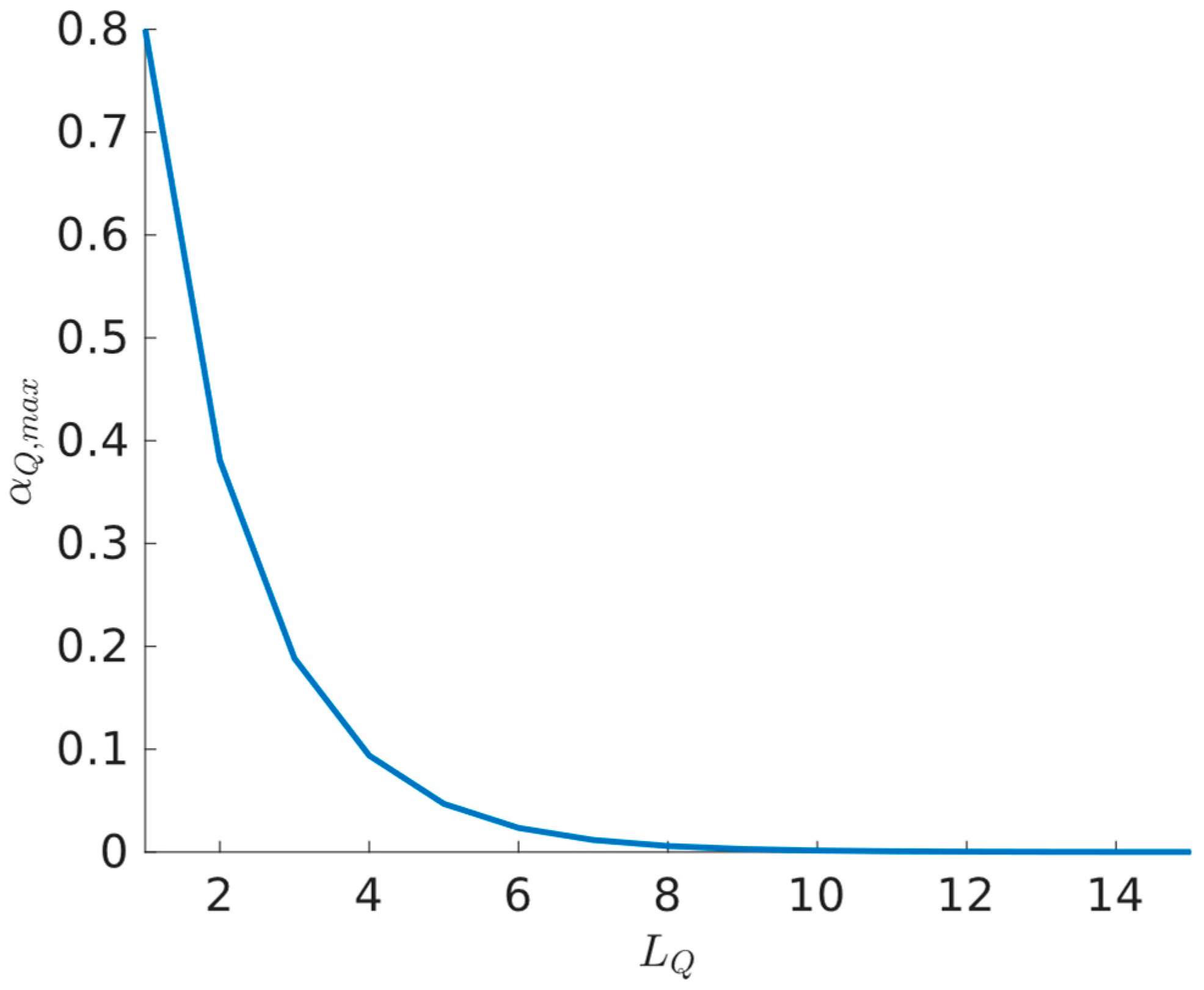
4.4. Results Interpretation

According to (69) and (79), as the number of hidden layers increases, the upper bounds for the learning rates ${\alpha }_Q$ and ${\alpha }_C$ decrease. This is due to the denominators in (69) and (79) being larger than their respective numerators, primarily because the denominators include squared terms. Therefore, the number of hidden layers in both neural networks is inversely proportional to the magnitude of their respective learning rates. For illustrative purposes, the action value function learning rate bound ${\alpha }_{Q,max}$ was plotted along the hidden layers $L_Q=1:15$ in Figure 1, based on (69). The norm bounds of the weights were selected as ${\overline{\mathit{W}}}_{Q, max}={\widehat{\mathit{W}}}_{Q, max}=2$ and ${\varphi }_{Q,max}={\dot{\varphi }}_{Q,max}=1$ for the activation function $\varphi \left(·\right)=\mathit{tanh}\left(·\right)$.

Remark 2.

This inversely proportional relationship between the number of NN hidden layers and the learning rate can be attributed to the gain in complexity of the NN optimization surface as the number of hidden layer increases. A high learning rate in such a scenario can lead to erratic updates in the intricate optimization surface, potentially causing the divergence of the learning process. While a smaller learning rate increases the risk of getting stuck in local minima, it is beneficial for a stable learning.

5. Simulation Study

Next, the impact of employing multiple hidden layers in the NN approximators, batch learning, and offline computation in the ADHDP learning process, namely the BOADHDP algorithm from Section 3.3, was tested on an ORM tracking task on the TRAS system. First, the system is described along with the data collection settings for BOADHDP. This is followed by a comparison between the BOADHDP learning process using single-hidden-layer NNs and the one using two-hidden-layer NNs for approximating the action value function and the controller. Finally, the online adaptive ADHDHP algorithms from [21,22] are compared with BOADHDP, highlighting the advantages of the latter.

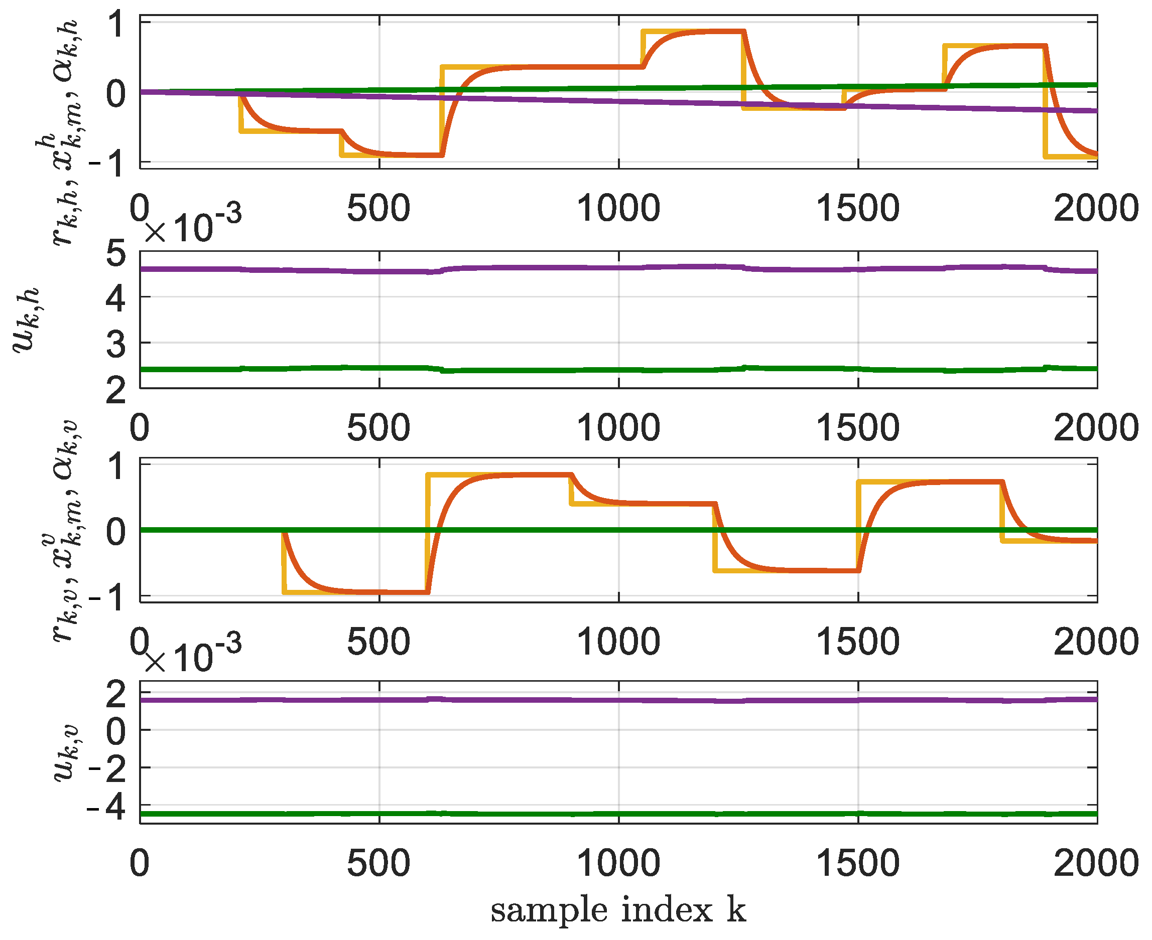
5.1. Data Collection Settings on TRAS System

The nonlinear system was characterized as a two-input and two-output system. The horizontal motion, or azimuth, operates as an integrator, whereas the vertical, or pitch, motion experiences different gravitational effects when moving upward versus downward. There was also an interconnection between these two channels. In Figure 2, a system setup is shown. The model used was a simplified deterministic continuous-time state-space representation, consisting of two interconnected state-space subsystems:

$$\left\{\begin{array}{c}{\dot{\omega }}_h={\displaystyle \frac{\left(sat\left(U_h\right)-M_h\left({\omega }_h\right)\right)}{2.7}}·{10}^{-5},\\ K_h=\left(0.216F_h\left({\omega }_h\right)\cos {\alpha }_v-0.058{\mathsf{\Omega }}_h+0.0178sat\left(U_v\right)\cos {\alpha }_v\right),\\ {\mathsf{\Omega }}_h={\displaystyle \frac{K_h}{\left(0.0238·{\cos }^2{\alpha }_v+3·{10}^{-3}\right)}},\\ {\dot{\alpha }}_h={\mathsf{\Omega }}_h,\\ {\dot{\omega }}_v={\displaystyle \frac{\left(sat\left(U_v\right)-M_v\left({\omega }_v\right)\right)}{1.63}}·{10}^{-4},\\ {\dot{\mathsf{\Omega }}}_v={\displaystyle \frac{1}{0.03}}\left(\begin{array}{c}0.2F_v\left({\omega }_v\right)-0.0127{\mathsf{\Omega }}_v-0.0935\sin {\alpha }_v\\ -9.28·{10}^{-6}{\mathsf{\Omega }}_v\left|{\omega }_v\right|+4.17·{10}^{-3}sat\left(U_h\right)-0.05\cos {\alpha }_v\\ -0.021{\mathsf{\Omega }}_h^2\sin {\alpha }_v\cos {\alpha }_v-0.093\sin {\alpha }_v+0.05\end{array}\right),\\ {\dot{\alpha }}_v={\mathsf{\Omega }}_v,\end{array}\right.$$

(80)

where $sat\left(\right)$ is the saturation function in the interval $\left[-1; 1\right]$. The horizontal azimuth control input was $U_h=u_1$ and the vertical pitch control was $U_v=u_2$. The system output was represented by the azimuth angle ${\alpha }_h\in \left[-\pi ;\pi \right]$ and by the pitch angle ${\alpha }_v\in \left[-\pi /2; \pi /2\right]$. Nonlinear static characteristics were derived from experimental data through polynomial fitting as in [29]:

$$M_v\left(\omega \right)=9.05\times {10}^{-12}{\omega }_v^3+2.76\times {10}^{-10} {\omega }_v^2+1.25\times {10}^{-4} {\omega }_v^1+1.66\times {10}^{-4},$$

(81)

$$\begin{array}{c}{F}_v\left(\omega \right)=-1.8\times {10}^{-18} {\omega }_v^5-7.8\times {10}^{-16} {\omega }_v^4+4.1\times {10}^{-11} {\omega }_v^3+2.7\times {10}^{-8} {\omega }^2\\ +3.5\times {10}^{-4} \omega -0.014,\end{array}$$

(82)

$$\begin{array}{c}{M}_h\left({\omega }_h\right)=5.95\times {10}^{-13} {\omega }_h^3-5.05\times {10}^{-10} {\omega }_h^2+1.02\times {10}^{-4} {\omega }_h^1\\ +1.61\times {10}^{-3} {\omega }_h,\end{array}$$

(83)

$$\begin{array}{c}{F}_h\left({\omega }_h\right)=-2.56\times {10}^{-20} {\omega }_h^5+4.09\times {10}^{-17} {\omega }_h^4+3.16\times {10}^{-12} {\omega }_h^3\\ -7.34\times {10}^{-9} {\omega }_h^2+2.12\times {10}^{-5} {\omega }_h+9.13\times {10}^{-3}.\end{array}$$

(84)

The process was discretized by using a zero-order hold sampler on both inputs and outputs. With a sampling time of $T_s=0.1 \mathrm{s}$, the following discrete-time model was obtained,

$$\left\{\begin{array}{c}{\mathit{x}}_{k+1}=f\left({\mathit{x}}_k,{\mathit{u}}_k\right),\\ {\mathit{y}}_k=g\left({\mathit{x}}_k\right)={\left[{\alpha }_{k,h},{\alpha }_{k,v}\right]}^T,\end{array}\right.$$

(85)

where the system state was ${\mathit{x}}_k={\left[{\omega }_{k,h},{\mathsf{\Omega }}_{k,h},{\alpha }_{k,h},{\omega }_{k,v},{\mathsf{\Omega }}_{k,v},{\alpha }_{k,v}\right]}^T\in {\mathfrak{R}}^6$ and the control input was ${\mathit{u}}_k=\left[u_{k,h},u_{k,v}\right]$, as in [29].

In the ORM tracking paradigm, the controlled system outputs track the output of the ORM model. In this application, the ORM was defined as in [29] and had the form of

$$\left\{\begin{array}{c}{x}_{k+1,m}^h=0.9673x_{k,m}^h+0.0328r_{k,h},\\ x_{k+1,m}^v=0.9673x_{k,m}^v+0.0328r_{k,v},\\ y_{k,m}={\left[y_{k,m}^h,y_{k,m}^v\right]}^T={\left[x_{k,m}^h,x_{k,m}^v\right]}^T,\end{array}\right.$$

(86)

where $r_{k,h}$ and $r_{k,v}$ are step input reference signals. Therefore, an extended state that comprises both the TRAS and the ORM states was defined as ${\mathit{x}}_k^e={\left[{\omega }_{k,h},{\mathsf{\Omega }}_{k,h},{\alpha }_{k,h},{\omega }_{k,v},{\mathsf{\Omega }}_{k,v},{\alpha }_{k,v},x_{k,m}^h,x_{k,m}^v,r_{k,h},r_{k,v}\right]}^T\in {\mathfrak{R}}^{10}$.

For data collection, the linear diagonal controller

$$C\left(z,\mathit{\theta }\right)=\left[\begin{array}{cc}{P}_{11}\left(z\right)/\left(1-z^{-1}\right)& 0\\ 0& P_{22}\left(z\right)/\left(1-z^{-1}\right)\end{array}\right],$$

$$P_{11}\left(z\right)=2.9341-5.8689z^{-1}+3.9303z^{-2}-0.9173z^{-3}-0.0777z^{-4},$$

$$P_{22}\left(z\right)=0.6228-1.1540z^{-1}+0.5467z^{-2}$$

(87)

was used in a closed loop with system (85), where the controller parameters were tuned using VRFT as in [29]. Having the closed loop stabilized, the successive step referenced input signals with amplitudes ranging in an interval of $r_{k,h}\in \left[-2;2\right]$, and $r_{k,v}\in \left[-1.4;1.1\right]$ were generated at $17$ s and $25$ s for the azimuth and pitch respectively. To guarantee a satisfactory exploration of the system’s state-space domain, a random noise was added at each two timesteps. The random noise added on $C_{11}\left(Z\right)$ had an amplitude of $\left[-1.6;1.6\right]$ and the one added on $C_{22}\left(Z\right)$ had an amplitude of $\left[-1.7;1.7\right]$. A total of $M=\mathrm{50,000}$ transitions were collected, creating, therefore, the dataset $D_{\mathrm{50,000}}=\left\{\right({\mathit{x}}_k^e, {\mathit{u}}_k,r\left({\mathit{x}}_k^e,{\mathit{u}}_k\right), {\mathit{x}}_{k+1}^e\left)\right\}$, with $k=1:\mathrm{50,000}$. An excerpt of the data exploration is shown in Figure 3. Next, BOADHDP was issued for action value function and controller NN approximations for both the single-hidden-layer ($L_Q=1$, $L_C=1$) and the multilayer case ($L_Q=2$, $L_C=2$).

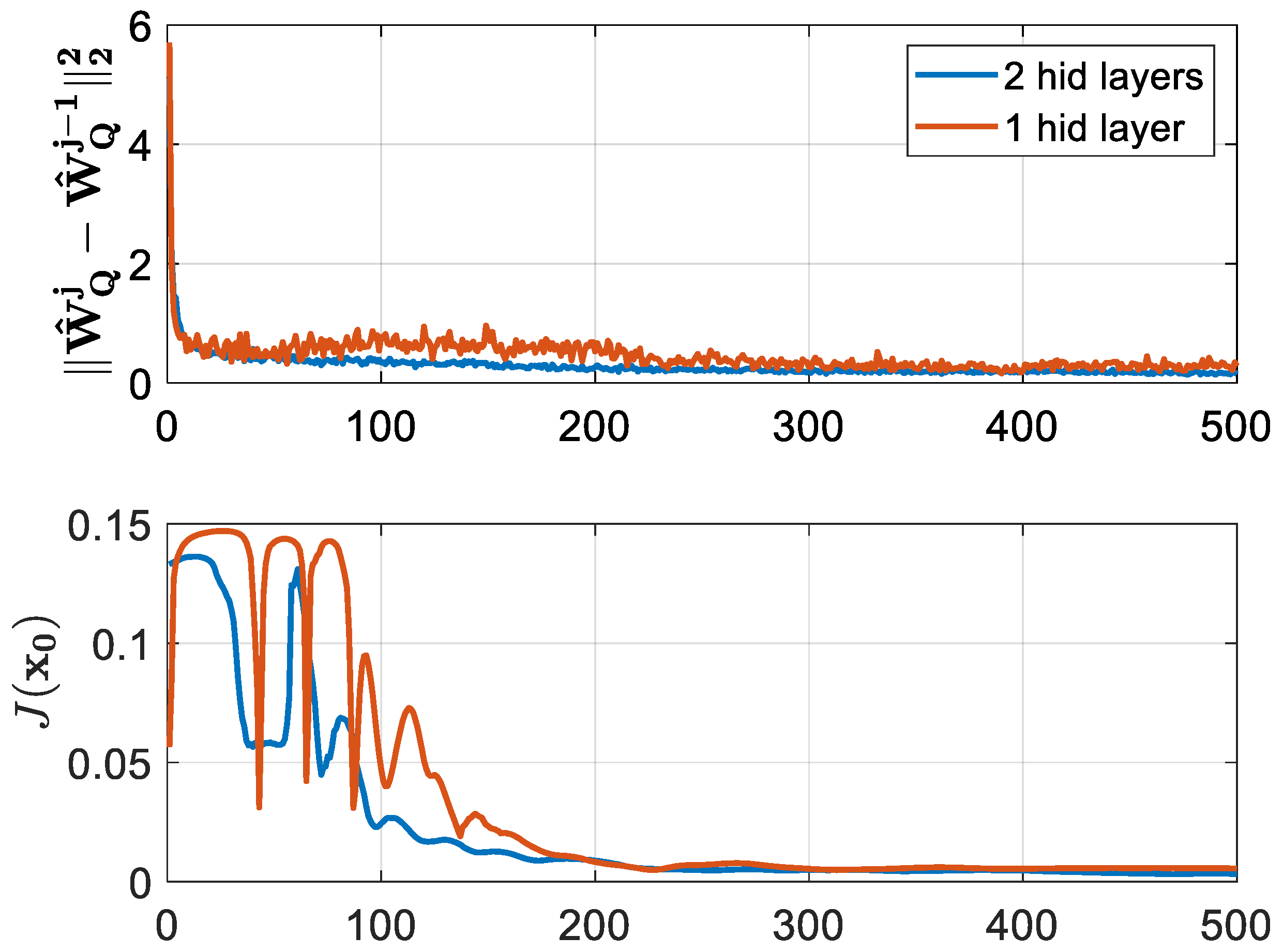
5.2. Comparison of BOADHDP with Single-Layer and Multilayer NN Approximations

For the single-layer NNs, the form of the action value function was 12-50-1 and that of the controller was 10-10-2. The activation functions of the hidden layer were hyperbolic tangents and the ones of the output layer were linear. The weights were initialized using the Xavier initialization [29]. The internal gradient updates were ${\mathsf{{\rm I}}}_{\mathrm{Q}}=500$ and ${\mathsf{{\rm I}}}_{\mathrm{C}}=100$ and the learning rates were selected to be ${\alpha }_Q=0.01$ and ${\alpha }_C=0.001$. The penalty function took the form of $r\left({\mathit{x}}_k^e,{\mathit{u}}_k\right)={\left({\alpha }_{k,h}-x_{k,m}^h\right)}^2+{\left({\alpha }_{k,v}-x_{k,m}^v\right)}^2$. The algorithm ran for a total number of 500 iterations. The performance of the NN controller was tested on a simulated scenario. In this scenario, the tracking capabilities were tested on a random reference signal generated from $[-1;1]$ for 2000 timesteps. Therefore, at each BOADHDP $j^{th}$ iteration, the performance of the controller was measured by the function $J\left({\mathit{x}}_k^e\right)={\left({\alpha }_{k,h}-x_{k,m}^h\right)}^2+{\left({\alpha }_{k,v}-x_{k,m}^v\right)}^2/2000$ on the simulated scenario, for $k=1:2000$. The convergence of the action value function and the values of $J\left({\mathit{x}}_k\right)$ is shown in Figure 4 in an orange color. This was computed by checking the norm between the weights from successive BOADHDP iterations, namely the norm ${‖{\widehat{\mathit{W}}}_Q^j-{\widehat{\mathit{W}}}_Q^{j-1}‖}_2^2$. The decreasing behavior of the successive weight norms from the first plot in Figure 4 proves the convergence of the action value function. The second plot presents the performance of the value function $J\left({\mathit{x}}_k^e\right)$ under the simulated scenario for the controller obtained from each iteration $j$, namely $C_j\left({\mathit{x}}_k^e,{\mathit{W}}_C\right)$. The tracking performance of the controller obtained at iteration $j=500$ is shown in Figure 5. In this figure, the performance of the TRAS system (85) in a closed loop with the controller $C_{500}\left({\mathit{x}}_k^e,{\mathit{W}}_C\right)$ is shown. The evolution in time of the output of the horizontal and the vertical axes is plotted in a blue color along with the reference signal (yellow) and reference model (orange), showing the tracking capacity of the $C_{500}\left({\mathit{x}}_k^e,{\mathit{W}}_C\right)$ controller.

For the multilayer NN setup, the form of the action value function was 15-50-10-2 and that of the controller was 10-10-4-2. The activation functions of the two hidden layers were hyperbolic tangents and the ones from the output layer were linear. The weights were initialized using the Xavier initialization [29]. The internal gradient updates were ${\mathsf{{\rm I}}}_{\mathrm{Q}}=500$ and ${\mathsf{{\rm I}}}_{\mathrm{C}}=100$, and the learning rates took the values of ${\alpha }_Q=0.01$ and ${\alpha }_C=0.001$. The algorithm ran for a total number of 500 iterations. The convergence of the action value function and the values of $J\left({\mathit{x}}_k\right)$ is shown in Figure 4 in a blue color. The tracking performance of the controller obtained at iteration $j=500$ is shown in Figure 5.

From Figure 4, it can be seen that the convergence of the two-layer NN approximators for the action value function and the controller delivered more stable results. First, the norm of the action value function successive weight differences from the first plot was less noisy and provided a faster convergence in the two-layer case than the single-layer NN. Then, in the second plot, the function $J\left({\mathit{x}}_k^e\right)$ converged faster to a lower value that correlated with a performant controller. Also, the values of $J\left({\mathit{x}}_k^e\right)$ was $0.0049$ for the single-layer NNs and $0.0031$ for the two-layer implementation. The two-layer implementation outperformed the single-layer one by 1.58%. The difference in tracking performance can be seen in Figure 5 and Figure 6, where the horizontal motion tracking improved in the case of the two-layer NN controller.

5.3. Comparison Between BOADHDP and the Online Adaptive ADHDP

Next, the online adaptive ADHDP algorithms from [21,22] were applied to the TRAS system. The difference between ADHDP methods [] was that the former one only updates the weights from the hidden to the output layer, while the latter updates the entire NN weights.

For these algorithms, we used the same NN architectures as in the single-layer NN from BOADHDP, namely the form of the action value function NN was 12-50-1 and that of the controller was 10-10-2. The activation functions of the hidden layer were hyperbolic tangents and the ones of the output layer were linear. The weights were also initialized using the Xavier initialization [29]. The learning rates were selected to be ${\alpha }_Q=0.01$ and ${\alpha }_C=0.001$. The penalty function took the form of $r\left({\mathit{x}}_k^e,{\mathit{u}}_k\right)={\left({\alpha }_{k,h}-x_{k,m}^h\right)}^2+{\left({\alpha }_{k,v}-x_{k,m}^v\right)}^2$.

Compared with BOADHDP, in these implementations, the adaptation of the NNs was made online, using only the transitions along with each time step of the simulated system. The algorithm ran for 200,000 time steps. Every 2000 steps, the controller weights were fixed and their performance was measured by the function $J\left({\mathit{x}}_k^e\right)={\left({\alpha }_{k,h}-x_{k,m}^h\right)}^2+{\left({\alpha }_{k,v}-x_{k,m}^v\right)}^2/2000$ under a simulated scenario, for $k=1:2000$. The convergence of the action value function and of the controller performance of the simulated scenario can be seen in Figure 7 for the ADHDP algorithms from [21,22]. The tracking performance of the ADHDP algorithms from [21,22] on the TRAS system using the aforementioned learning settings is presented in Figure 8. The value of the $J\left({\mathit{x}}_k^e\right)$ was $0.0236$ for the ADHDP algorithm from [21] and $0.0258$ for the ADHDP algorithm from [22].

The $J\left({\mathit{x}}_k^e\right)$ values of the BOADHDP and ADHDP algorithms from [21,22] are summarized in

Table 1. Comparison between the BOADHDP (single- and multiple-hidden-layer NN approximations) and the ADHDP algorithms from [21,22].

Algorithm	$\mathit{J}\left({\mathit{x}}_{\mathit{k}}^{\mathit{e}}\right)$
BOADHDP with NN approximation having a single hidden layer	$0.0049$
BOADHDP with NN approximation having two hidden layers	$0.0031$
ADHDP from [21]	0.0236
ADHDP from [22]	0.0258

. Also, from Figure 5 and Figure 8, it can be observed that the online adaptive ADHDP algorithms could not deliver the same performance as their batch and offline counterpart, BOADHDP. Furthermore, the ADHDP algorithms presented in [21,22] failed to enhance controller performance, even though they utilized four times as many collected transitions from the system. This difference in the performance of the BOADHDP algorithm stems, in part, from the batch nature of the learning process. By processing multiple collected transitions from the state action space at the same time during NN actualization, the gradient for the action value and controller NNs is averaged over all the transitions. In turn, this makes the NN update more stable. By issuing the gradient update in an offline manner, the same collected transitions are used at each iteration, making the convergence speed faster. This stands in accordance with the observations from [28], where the authors proved the advantages of batch learning in comparison to the online adaptive single-transition learning from the classical ADHDP methods. Also, from this case study, it can be seen that the number of transitions required for learning was higher in the online adaptive case than in the batch offline case.

6. Discussion and Conclusions

In this paper, we study the theoretical stability of BOADHDP with deep neural networks as function approximators for the action value function and the controller. To this end, we introduce a stability criterion for the iteratively updated action value function and controller NN. The theory uses the Lyapunov stability approach and shows that the weight estimation errors are UUB if some inequality constraints on the learning rate magnitudes are respected. This research extends the previous results from the literature, such as [21,22], both theoretically and practically.

• First, our Lyapunov stability is extended to address NN approximators for action value functions and controllers with multiple hidden layers. Although NNs with a single hidden layer are universal approximators, their usage for highly nonlinear applications is hindered by their generalization capabilities. In contrast, multilayer NNs can learn complex features effectively, reducing overfitting and generalization issues. The results outlined in Theorem 1 indicate also an indirect proportionality between the number of NN hidden layers and the magnitude of the learning rate, providing a practical heuristic approach for practical ADP applications of multilayer NNs.
• Second, our theoretical Lyapunov stability analysis addresses the usage of batch offline learning of the action value function and controller NNs. Although successful ADP applications have been reported using adaptive update methods, their practical use is often constrained by the significant number of iterations required for convergence. The adoption of batch learning has, thus, become standard practice, necessitating a theoretical Lyapunov stability coverage.
• Finally, from a practical point of view, we validate the advantage of using BOADHDP with multilayer NNs through a case study on a twin rotor aerodynamical system (TRAS). This study compares BOADHDP using neural networks with a single layer and two hidden layers as function approximators. The results show that the normed action value function weight convergence is smoother with two-hidden-layer networks, also leading to a controller with an enhanced performance on the control benchmark ($0.0049$ for the single-layer NNs and $0.0031$ for the two-layer implementation, namely a $1.58\%$ improvement). This demonstrates the superior capability of multilayer networks in managing complex, nonlinear control systems. Also, BOADHDP is compared with ADHDP algorithms from [21,22], with ADHDP algorithms from [21,22] obtaining $0.0236$ and $0.0258$, respectively, on the control benchmark, while also requiring four times more collected transitions from the TRAS system. This proves both the efficiency of the BOADHDP with respect to the number of collected transitions and the performance of using batch offline learning methodologies, confirming the results from [28].

Our findings highlight the advantages of BOADHDP with deep neural networks in practical applications, underscoring the improved stability and performance in control tasks. Future research may explore extending this batched multilayer approach to adaptive learning scenarios. From a practical point of view, applications entailing deep neural networks and batch learning applications might benefit from this analysis.

References

1. Werbos, P.J. Beyond Regression: New Tools for Prediction and Analysis in the Behavioral Science. Ph.D. Thesis, Committee on Applied Mathematics, Harvard University, Cambridge, MA, USA, 1974. [Google Scholar]
2. Bellman, R.E. Dynamic Programming; Princeton University Press: Princeton, NJ, USA, 1957. [Google Scholar]
3. Werbos, P.J. Approximate dynamic programming for real time control and neural modeling. In Handbook of Intelligent Control: Neural, Fuzzy, and Adaptive Approaches; White, D.A., Sofge, D.A., Eds.; Van Nostrand Reinhold: New York, NY, USA, 1992; pp. 493–525. [Google Scholar]
4. Al-Tamimi, A.; Lewis, F.L. Discrete-time nonlinear HJB solution using approximate dynamic programming: Convergence proof. IEEE Trans. Syst. Man Cybern. B 2008, 38, 943–949. [Google Scholar] [CrossRef] [PubMed]
5. Prokhorov, D.V.; Wunsch, D.C. Adaptive critic designs. IEEE Trans. Neural Netw. 1997, 8, 997–1007. [Google Scholar] [CrossRef] [PubMed]
6. Liu, X.; Balakrishnan, S.N. Convergence analysis of adaptive critic based optimal control. In Proceedings of the American Control Conference, Chicago, IL, USA, 28–30 June 2000. [Google Scholar]
7. White, D.A.; Sofge, D.A. Handbook of Intelligent Control: Neural, Fuzzy, and Adaptive Approaches; Van Nostrand Reinhold: New York, NY, USA, 1992. [Google Scholar]
8. Padhi, R.; Unnikrishnan, N.; Wang, X.; Balakrishnan, S.N. A single network adaptive critic (SNAC) architecture for optimal control synthesis for a class of nonlinear systems. Neural Netw. 2006, 19, 1648–1660. [Google Scholar] [CrossRef] [PubMed]
9. Balakrishnan, S.N.; Biega, V. Adaptive-critic-based neural networks for aircraft optimal control. J. Guid. Control Dyn. 1996, 19, 893–898. [Google Scholar] [CrossRef]
10. Dierks, T.; Jagannathan, S. Online optimal control of affine nonlinear discrete-time systems with unknown internal dynamics by using time-based policy update. IEEE Trans. Neural Netw. Learn. Syst. 2012, 23, 1118–1129. [Google Scholar] [CrossRef] [PubMed]
11. Venayagamoorthy, G.K.; Harley, R.G.; Wunsch, D.C. Comparison of heuristic dynamic programming and dual heuristic programming adaptive critics for neurocontrol of a turbogenerator. IEEE Trans. Neural Netw. 2002, 13, 764–773. [Google Scholar] [CrossRef] [PubMed]
12. Ferrari, S.; Stengel, R.F. Online adaptive critic flight control. J. Guid. Control Dyn. 2004, 27, 777–786. [Google Scholar] [CrossRef]
13. Ding, J.; Jagannathan, S. An online nonlinear optimal controller synthesis for aircraft with model uncertainties. In Proceedings of the AIAA Guidance, Navigation and Control Conference, Toronto, ON, Canada, 2–5 August 2010. [Google Scholar]
14. Vrabie, D.; Pastravanu, O.; Lewis, F.; Abu-Khalaf, M. Adaptive optimal control for continuous-time linear systems based on policy iteration. Automatica 2009, 45, 477–484. [Google Scholar] [CrossRef]
15. Dierks, T.; Jagannathan, S. Optimal control of affine nonlinear continuous-time systems. In Proceedings of the American Control Conference, Baltimore, MA, USA, 30 June–2 July 2010. [Google Scholar]
16. Vamvoudakis, K.; Lewis, F. Online actor-critic algorithm to solve the continuous-time infinite horizon optimal control problem. Automatica 2010, 46, 878–888. [Google Scholar] [CrossRef]
17. Enns, R.; Si, J. Helicopter trimming and tracking control using direct neural dynamic programming. IEEE Trans. Neural Netw. 2003, 14, 929–939. [Google Scholar] [CrossRef]
18. Liu, D.; Javaherian, H.; Kovalenko, O.; Huang, T. Adaptive critic learning techniques for engine torque and air–fuel ratio control. IEEE Trans. Syst. Man Cybern. B 2008, 38, 988–993. [Google Scholar]
19. Ruelens, F.; Claessens, B.J.; Quaiyum, S.; De Schutter, B.; Babuška, R.; Belmans, R. Reinforcement learning applied to an electric water heater: From theory to practice. IEEE Trans. Smart Grid 2018, 9, 3792–3800. [Google Scholar] [CrossRef]
20. He, P.; Jagannathan, S. Reinforcement learning-based output feedback control of nonlinear systems with input constraints. IEEE Trans. Syst. Man Cybern. B 2005, 35, 150–154. [Google Scholar] [CrossRef] [PubMed]
21. Liu, F.; Sun, J.; Si, J.; Guo, W.; Mei, S. A boundness result for the direct heuristic dynamic programming. Neural Netw. 2012, 32, 229–235. [Google Scholar] [CrossRef] [PubMed]
22. Sokolov, Y.; Kozma, R.; Werbos, L.D.; Werbos, P.J. Complete stability analysis of a heuristic approximate dynamic programming control design. Automatica 2015, 59, 9–18. [Google Scholar] [CrossRef]
23. Mnih, V.; Kavukcuoglu, K.; Silver, D.; Rusu, A.A.; Veness, J.; Bellemare, M.G.; Graves, A.; Riedmiller, M.; Fidjeland, A.K.; Ostrovski, G.; et al. Human-level control through deep reinforcement learning. Nature 2015, 518, 529–533. [Google Scholar] [CrossRef]
24. Lillicrap, T.; Hunt, J.; Pritzel, A.; Heess, N.; Erez, Y.; Tassa, Y.; Silver, D.; Wierstra, D. Continuous control with deep reinforcement learning. In Proceedings of the International Conference on Learning Representations, San Juan, Puerto Rico, 2–4 May 2016. [Google Scholar]
25. Fujimoto, S.; Hoof, H.; Meger, D. Addressing function approximation error in actor-critic methods. In Proceedings of the Internation Conference on Machine Learning, Stockholmsmässan, Stockholm, Sweden, 10–15 July 2018. [Google Scholar]
26. Riedmiller, M. Neural Fitted Q Iteration–First Experiences with a Data Efficient Neural Reinforcement Learning Method. In Proceedings of the European Conference on Machine Learning, Porto, Portugal, 3–7 October 2005. [Google Scholar]
27. Radac, M.-B.; Lala, T. Learning output reference model tracking for higher-order nonlinear systems with unknown dynamics. Algorithms 2019, 12, 121. [Google Scholar] [CrossRef]
28. Watkins, C. Learning from Delayed Rewards. Ph.D. Thesis, Department of Computational Science, University of Cambridge, Cambridge, UK, 1989. [Google Scholar]
29. Glorot, X.; Bengio, Y. Understanding the difficulty of training deep feedforward neural networks. In Proceedings of the Thirteenth International Conference on Artificial Intelligence and Statistics, Sardinia, Italy, 13–15 May 2010. [Google Scholar]
Figure 1. Relation between the number of NN layers and the bound of the learning rate α Q , m a x .
Mathematics 13 00206 g001
Figure 2. TRAS system setup [29].
Mathematics 13 00206 g002
Figure 3. Data collection in relation to the TRAS system: r k , h and r k , v (yellow); x k , m h and x k , m v (red); α k , h and α k , v (blue).
Mathematics 13 00206 g003
Figure 4. BOADHDP convergence in the TRAS system.
Mathematics 13 00206 g004
Figure 5. One-hidden-layer controller learned through BOADHDP, at iteration j = 500 : r k , h and r k , v (yellow); x k , m h and x k , m v (red); α k , h and α k , v (blue). The commands u k , h and u k , v are for the horizontal and vertical axes (blue).
Mathematics 13 00206 g005
Figure 6. Two-hidden-layer controller learned through BOADHDP, at iteration j = 500 : r k , h and r k , v (yellow); x k , m h and x k , m v (red); α k , h and α k , v (blue). The commands u k , h and u k , v are for the horizontal and vertical axes (blue).
Mathematics 13 00206 g006
Figure 7. ADHDP convergence in relation to the TRAS system. ADHDP algorithm from [21] in purple and ADHDP algorithm from [22] in green.
Mathematics 13 00206 g007
Figure 8. Tracking performance of the ADHDP algorithms from [21,22], at iteration j = 150,000 : r k , h and r k , v (yellow); x k , m h and x k , m v (red); α k , h and α k , v (green—ADHDP algorithm from [21], purple—ADHDP algorithm from [22]). The commands u k , h and u k , v are for the horizontal and vertical axes (green—ADHDP algorithm from [21], purple—ADHDP algorithm from [22]).
Mathematics 13 00206 g008