Abstract
Accurate traffic flow prediction plays a vital role in intelligent transportation systems, helping traffic management departments maintain stable traffic order, reduce traffic congestion, and improve road safety. Existing prediction methods focus on dynamic modeling of the spatiotemporal dependencies of traffic flow, capturing the periodicity and spatial heterogeneity in traffic data. However, they still suffer from a lack of focus on the important local information in long-term predictions, leading to overly smooth results that fail to effectively capture sudden changes in traffic patterns. To address these limitations, we propose the sLSTM-Attention-Based Multi-Head Dynamic Graph Convolutional Network (sAMDGCN) model. Specifically, we extend sLSTM and introduce temporal trend-aware multi-head attention to jointly capture the complex temporal dependencies. We propose a multi-head dynamic graph convolutional network to capture a wider range of dynamic spatial dependencies. To validate the effectiveness of sAMDGCN, we perform extensive experiments on four real-world traffic flow datasets. Experimental results show that our proposed sAMDGCN model outperforms the advanced baseline methods in long-term traffic flow prediction tasks, demonstrating its superior performance in capturing complex and dynamic traffic patterns.
Keywords:
traffic flow prediction; spatiotemporal dependency; sLSTM; attention; graph convolutional network MSC:
68T01
1. Introduction
The rapid acceleration of global urbanization has led to a significant increase in vehicle usage, making traffic congestion a widespread issue. In response, many countries are actively developing Intelligent Transportation Systems (ITS) [1], leveraging advanced technologies to optimize traffic route planning and minimize congestion. As a core technology in ITS, traffic flow prediction plays a crucial role by analyzing future traffic patterns based on recent conditions and historical data, enabling individuals to select less congested routes and enhancing traffic resource management and scheduling. To monitor road conditions, many cities have deployed a network of sensors that continuously collect traffic data, such as flow rates, average vehicle speeds, and road occupancy levels, at regular intervals. Supported by robust hardware, numerous methods have emerged to utilize these data for accurate traffic flow prediction.
Traffic flow prediction was initially treated as a typical time series prediction task, and statistical methods like Historical Average (HA) [2], Auto-Regressive Integrated Moving Average (ARIMA) [3], and Vector Autoregression (VAR) [4] were commonly applied. However, these methods rely on assumptions of stationarity and linearity, making them incapable of capturing the complex and dynamic nonlinear temporal dependencies inherent in real-world traffic, often resulting in significant prediction errors. To address these limitations, machine learning algorithms such as Support Vector Regression (SVR) [5] and K-Nearest Neighbors (KNNs) [6] were later introduced, enabling the modeling of more intricate traffic patterns and improving predictive accuracy. Despite these advancements, machine learning methods still struggle to fully overcome the constraints of linear assumptions. Furthermore, both statistical and machine learning approaches are hindered by their simplistic structures, as they primarily utilize local traffic information and fail to capture the broader, global patterns necessary for more robust traffic flow prediction.
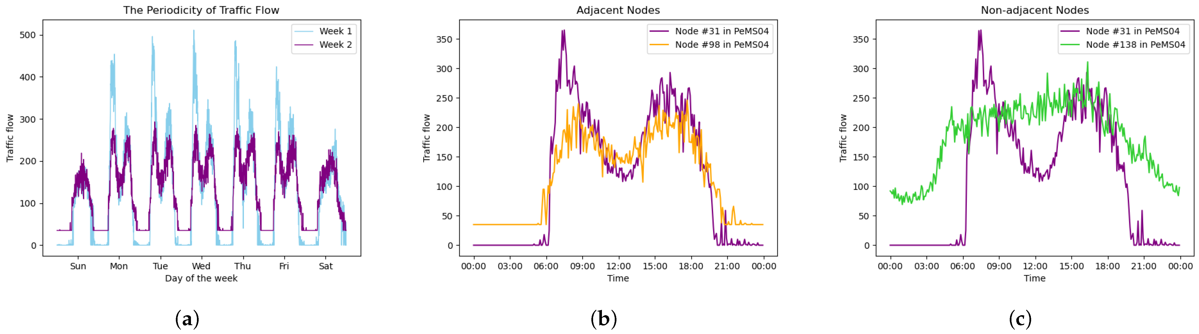
Traffic flow data exhibit strong periodicity, as patterns often repeat over time. For instance, weekday traffic typically features similar peaks due to commuting, and daytime traffic flow is usually higher than that at night. Figure 1a illustrates traffic flow data collected by a sensor on a California highway over two consecutive weeks. Although the peak values differ across weekdays, consistent peaks and troughs occur during the same periods, and the traffic patterns of the two weeks display striking similarities, reflecting clear periodicity. With the rise of deep learning, models equipped with large numbers of parameters and complex structures are now capable of capturing nonlinear dependencies and uncovering hidden patterns within sequences. Among these, Recurrent Neural Networks (RNNs) [7] have demonstrated significant potential in traffic flow prediction. The gating mechanism of RNNs endows them with memory capabilities, enabling them to effectively capture traffic flow periodicity and accurately forecast future trends. However, when applied to long-term prediction tasks, RNNs face challenges such as gradient explosion and vanishing. To address these issues, two RNN variants, Long Short-Term Memory (LSTM) [8,9] and Gated Recurrent Unit (GRU) [10], have been introduced, which alleviate these problems and further enhance long-term prediction performance. Later, the introduction of attention mechanisms and Transformer [11] have revolutionized the modeling of temporal dependencies, which aggregate features of the input sequence in parallel through weighted summation, outperforming RNN-based models in long-term predictions.
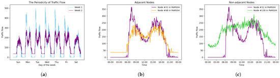
Figure 1.
Periodicity and spatial heterogeneity of traffic flow. (a) Traffic flow of node #31 in PeMS04 for two consecutive weeks. (b) Traffic flow of two adjacent nodes in a day. (c) Traffic flow of two non-adjacent nodes in a day.
Traffic flow data also exhibit spatial correlations. Adjacent roads tend to have similar traffic patterns, while roads farther apart may show spatial heterogeneity. For example, Figure 1b shows that two adjacent nodes on the same day have similar traffic trends, while Figure 1c shows significant differences in the patterns of two nodes that are farther apart. Inspired by this, Convolutional Neural Networks (CNNs) [12] were introduced for traffic flow prediction, treating the traffic network as 2D grids to capture spatial dependencies. However, the traffic network does not follow the traditional Euclidean space, and the distance between roads does not fully represent their connectivity. To overcome this, Graph Neural Networks (GNNs) [13], which effectively capture non-Euclidean spatial features, were applied. Specifically, Graph Convolutional Networks (GCNs) [14], which apply convolution to graph structures, update the feature representation of the target node by aggregating the features of neighboring nodes, making full use of the spatial correlations within the traffic network and achieving great success in traffic flow prediction.
However, in traffic flow prediction, more recent historical data typically have a greater impact on future traffic patterns. Whereas, attention mechanisms assign equal importance to all time steps when aggregating features, which does not align with the realistic dynamics of traffic flow. Very recently, Scalar LSTM (sLSTM) [15] was proposed to make the important information occupy a significant proportion of the memory, demonstrating obvious advantages in language modeling tasks compared with state-of-the-art baselines and paving a new way for handling time sequences. Despite its superior performance in language modeling, the performance of sLSTM in traffic flow prediction tasks has yet to be investigated. Additionally, traditional GNN-based models fail to account for the dynamic nature of spatial correlations in traffic networks. Factors such as weather conditions, road closures, and traffic accidents can alter the connections between roads, and using static spatial models may lead to the propagation of inaccurate information. This limitation calls for more dynamic methods to model spatial dependencies, ensuring more accurate traffic flow predictions.
To address the aforementioned problems and inspired by [15,16], we propose a novel traffic flow prediction model named sLSTM-Attention-Based Multi-Head Dynamic Graph Convolutional Network (sAMDGCN), which follows the encoder–decoder structure. When modeling the temporal dependencies, we propose to use the sLSTM module in the encoder for feature extraction and use the Temporal Trend-aware Multi-head Attention (TTMA) module in the decoder to autoregressively generate prediction results. When modeling the spatial dependencies, we propose a Multi-head Dynamic Graph Convolutional Network (MDGCN) module to capture a wide range of dynamic spatial correlations. These modules together constitute our sAMDGCN model. The main contributions of this paper are summarized as follows:
- To capture complex and dynamic traffic patterns in long-term predictions, we propose a novel sAMDGCN model, which follows the encoder–decoder structure and consists of an sLSTM module, TTMA module, and MDGCN module.
- We extend sLSTM for solving traffic flow prediction tasks and combine it with TTMA to model temporal dependencies for the first time, capturing dynamic traffic patterns while focusing on key historical information. An MDGCN module is proposed to capture the extensive dynamic spatial correlations in traffic networks.
- Extensive experiments on four real-world traffic flow datasets are conducted to validate the advanced performance of sAMDGCN, demonstrating its effectiveness across various traffic flow forecasting tasks.
This paper is organized as follows: We first introduce the related work of traffic flow prediction in Section 2. Then, we introduce the structure of the proposed sAMDGCN in detail in Section 3. Section 4 demonstrates the effectiveness of our model through extensive comparison experiments and ablation experiments. Finally, the conclusions are drawn and future work are discussed in Section 5.
2. Related Work
Traditional Temporal Dependency Modeling. Traffic flow prediction is often treated as a time series prediction task. Traditional methods like Historical Average (HA) [2], Auto-Regressive Integrated Moving Average (ARIMA) [3], and Vector Autoregression (VAR) [4] relied on statistical models, and they struggled with dynamic and nonlinear patterns due to the reliance on stationarity and linearity assumptions. Machine learning methods, such as Support Vector Regression (SVR) [5] and K-Nearest Neighbors (KNNs) [6], improved on these by reducing the reliance on linearity but were limited to short-term forecasts due to a lack of memory capabilities. With the rise of deep learning, Recurrent Neural Networks (RNNs) introduced memory functions, enabling long-term predictions. However, RNNs suffer from gradient issues, leading to the adoption of improved models like Long Short-Term Memory (LSTM) [8,9] and Gated Recurrent Unit (GRU) [10], which use gating mechanisms to retain historical data. Overall, RNN-based models excel in long-term traffic flow prediction.
Static Spatial Correlation. Apart from the temporal features, traffic flow prediction tasks have spatial correlations, which can significantly improve the prediction accuracy. Convolutional Neural Networks (CNNs) were initially used to capture spatial dependencies by representing traffic networks as 2D grids. Later, hybrid models like CNN-LSTM [17,18] combined spatial and temporal information for better performance by considering both short-term fluctuations and long-term trends. However, CNN is based on the Euclidean space assumption, and traffic networks exhibit obvious non-Euclidean characteristics. To capture the non-Euclidean graph data structures, Graph Neural Networks (GNNs), particularly Graph Convolutional Networks (GCNs), were introduced to handle these structures and achieved superior performance [19,20,21,22,23,24,25]. In addition, some other models that take advantage of the graph structures, such as [26,27], have also shown good results in traffic flow prediction tasks. Compared with traditional temporal-dependent models, GNN-based spatiotemporal models can better extract correlations from both temporal and spatial dimensions of non-Euclidean topological data and offer higher prediction accuracy.
Attention-Based and Dynamic Spatiotemporal Correlation. RNNs struggle with long-range dependencies since they store information through weighted summation, which treats different time steps unequally, limiting their performance in tasks like long-term traffic flow prediction. Attention [11] mechanisms addressed this by allowing the model to focus on specific time steps and assign dynamic weights to them. MRA-BGCN [28] and A3T-GCN [29] combine attention with GCN, greatly improving the ability to capture dynamic correlations and enhancing the flexibility and robustness of long-term predictions. Traditional GNNs often rely on static adjacency matrices, but real-world factors affect the spatial correlations in traffic networks, making dynamic modeling of spatial features crucial for improving prediction accuracy. Building on this, ASTGNN [16] integrated dynamic GCN with the Transformer model to capture dynamic spatiotemporal correlations effectively. STTNs [30] introduced temporal and spatial Transformers, excelling at capturing long-term temporal dependencies and dynamic spatial correlations. STN-GCN [31] proposed a framework for spatial–temporal normalized graph convolutional neural networks. Given the success of these models, our approach also takes advantage of the attention mechanism and considers dynamic spatiotemporal correlations for better long-time traffic flow prediction.
3. Method
In this section, we first give the definition of the traffic flow prediction problem; then, we illustrate the overall framework of our sAMDGCN model.
3.1. Problem Definition
The essence of the traffic flow prediction problem lies in utilizing historical traffic data along with additional information to analyze the dynamic correlations within time series and predict future trends. In this study, historical traffic data refer to past traffic flow, while additional information includes the traffic network structure. Therefore, the traffic flow prediction problem addressed in this paper is defined as using both the historical traffic flow data and traffic network to forecast future traffic conditions.
Traffic Flow Sequence. The traffic flow information is a three-dimensional tensor , which represents the data of L time slices collected by N sensors on D attributes over a period of time. We divide the dataset into segments of length in the first dimension, and these segments can be further divided into historical sequences of length and label sequences of length . It is worth noting that is equal to the length of the predicted time steps . In addition, since only traffic flow changes significantly over time in the feature dimensions of the dataset, we only take attribute in the third dimension. After processing, we obtain several history sequences and label sequences .
Traffic Network. According to the spatial distribution of sensors, the traffic network can be constructed into an undirected graph , where represents the node set composed of N sensors and represents the connection relationship between sensors. Through the undirected graph , we can construct an adjacency matrix . If two nodes are connected, the element corresponding to A is set to 1; otherwise, it is set to 0. The adjacency matrix A obtained in this way can reflect the complex connections of the traffic network.
After obtaining the traffic flow history sequence and the adjacency matrix A, traffic flow prediction only needs to find a mapping model to predict the traffic flow sequence for the next T time steps, which can be expressed as follows:
where represents the learnable parameters of model .
3.2. Overall Framework
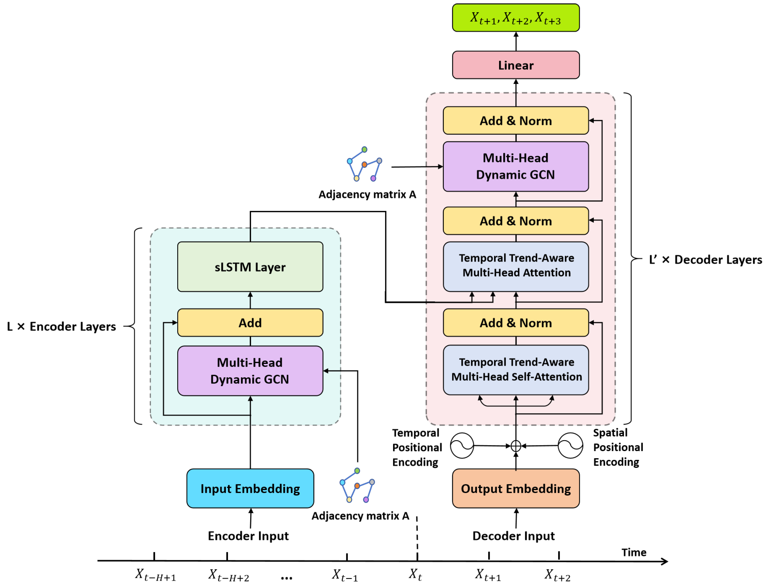
In this subsection, we will introduce the overall framework of our sAMDGCN model, as shown in Figure 2. Our sAMDGCN model adopts an encoder–decoder structure. The encoder extracts and processes the input sequence to obtain a new set of encoded sequences, while the decoder analyzes the encoded sequence and decodes it into a target sequence.

Figure 2.
The overall framework of our sAMDGCN model, which follows an encoder–decoder structure.
3.2.1. Encoder
As shown in Figure 2, the encoder is composed of a stack of identical layers, and each encoder layer consists of two basic modules, namely, the multi-head dynamic GCN (MDGCN) module and the sLSTM module. The MDGCN module is built upon GCN and used to aggregate the spatial information of nodes and capture the dynamic spatial correlations of traffic flow. The sLSTM module is introduced to summarize historical information and capture the dynamic temporal correlations of traffic flow across time steps.
Graph Convolutional Network (GCN). GCN propagates and aggregates the feature information of adjacent nodes through graph convolution, and then learns the embedded representation of each node. For undirected graphs, the core operation of GCN can be defined by (2).
where is the adjacency matrix with self-connection, i.e., . is the degree matrix of , and represents the normalized adjacency matrix. is the node representation of the l-th layer, ( and represent the input dimension and output dimension of GCN) is the learnable parameter matrix of the l-th layer, and represents the ReLU activation function. GCN can perform recursive calculations, but only a single calculation is considered in this work. For the convenience of description, the superscript indicating the layer will be omitted in the following.
Multi-Head Dynamic GCN (MDGCN). Traditional GCN is based on the static spatial correlations assumption. However, the factors affecting traffic flow are complex, and the static adjacency matrix cannot reflect the dynamic changes of spatial correlations. Therefore, we multiply the normalized adjacency matrix by a coefficient matrix , which is calculated by the node representation itself, as defined in (3).
This coefficient matrix can reflect the correlations between nodes. We integrate it with GCN to obtain a dynamic GCN (DGCN), which is denoted by (4).
Building on this, to extract more diverse dynamic spatial correlations, we introduce the multi-head mechanism. Specifically, we divide the d feature dimensions of the node representation into k parts, perform the DGCN operation on each part independently, and then concatenate all the results to obtain the final output of the MDGCN module. This can be expressed by (5).
To avoid gradient explosion and vanishing, we also include residual connections in MDGCN. Moreover, the module only needs to learn feature increments, which increases the flexibility and robustness of the model.
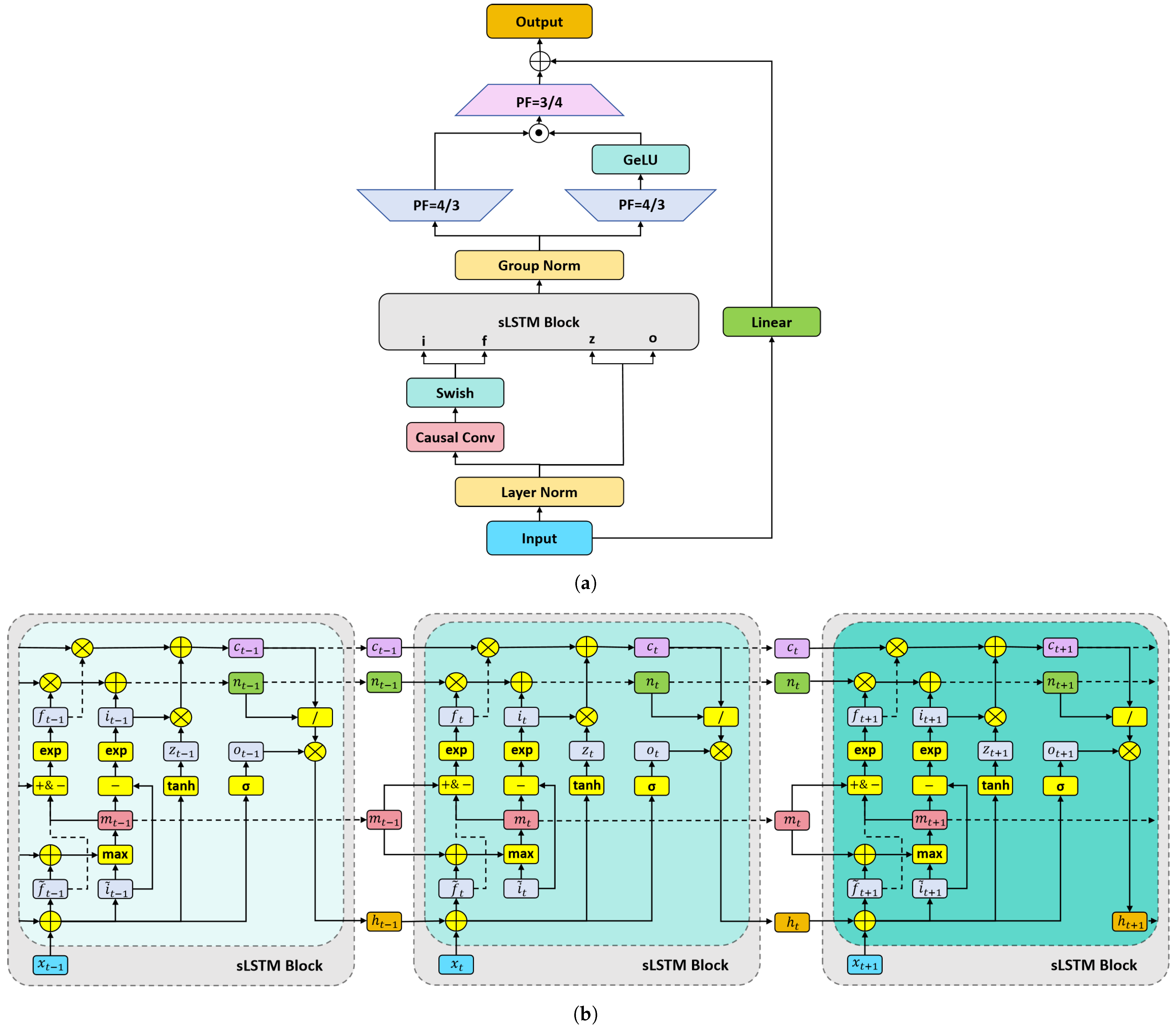
sLSTM Layer. sLSTM replaces the sigmoid activation function in the input gate and forget gate with an exponential activation function. This more aggressive strategy facilitates the retention of important information in the historical memory, allowing critical information to occupy a larger proportion of the memory. Additionally, sLSTM introduces more memory units, enhancing the diversity of the stored information. Furthermore, sLSTM incorporates a multi-head mechanism to capture dynamic temporal correlations across different subspaces. Given these features, sLSTM is highly effective at extracting features from input data across time steps, making it an ideal choice as the core module of the encoder in our model. The structure of the sLSTM module is shown in Figure 3.

Figure 3.
sLSTM module. (a) Overall structure. (b) Details of the sLSTM block.
As can be seen from Figure 3a, the input of the sLSTM module will form two branches after layer normalization. One branch will perform causal convolution and use the swish activation function; then, it will serve as the input of the input gate and the forget gate of the sLSTM block. The other branch directly serves as the input of the memory unit and the output gate of the sLSTM block. For the convenience of description, we will unify the input of the gate of the sLSTM block at time t as . The calculation process inside the sLSTM block can be expressed as follows:
where W and R with subscripts are weight matrices, b with subscripts are bias terms, is exponential activation function, is sigmoid activation function, is hyperbolic tangent activation function, and ⊙ is dot product. It is worth mentioning that sLSTM uses the exponential activation function in the calculation of the input gate and the forget gate instead of the sigmoid activation function used in conventional LSTM. The advantage of this exponential activation function is that if there is a sudden change in traffic flow at a certain time step, the rapidly changing gradient of the exponential activation function can amplify the importance of this time step in historical memory, thereby affecting the judgment of future traffic trends. Therefore, this characteristic of sLSTM helps the entire model respond quickly to sudden changes in traffic patterns.
After the input is recursively processed, as shown in Figure 3b, the hidden state h continues to participate in subsequent operations as the output of the sLSTM block. Group normalization is applied to the multi-head mechanism, where the calculation of multi-head sLSTM involves concatenating the results of multiple heads. The group-normalized hidden state is then split into two parts, which are each up-projected to capture the dynamic correlations of the original space in a nonlinear manner. One branch passes through a GeLU activation function, and the resulting output is dot-multiplied with the other branch, followed by down-projection back to the original space. Finally, a residual connection with linear projection is applied to obtain the output of the sLSTM module.
The output of the encoder layer has effectively summarized the historical information and captured both global and local spatiotemporal correlations. Stacking multiple encoder layers further enhances this capability, allowing the model to better capture complex, long-range dependencies and refine the feature representations for improved performance.
3.2.2. Decoder
The decoder is composed of spatiotemporal positional encoding and several stacked decoder layers, as shown in Figure 2. The decoder layer consists of two modules: temporal trend-aware multi-head attention (TTMA) and MDGCN. Since MDGCN has been introduced in Section 3.2.1, we will focus on the TTMA module and the spatiotemporal positional encoding here.
Temporal Trend-Aware Multi-Head Attention (TTMA). Inspired by [16], we integrate TTMA within our model. Traditional attention mechanism can be described as a process where values are weighted and summed based on the similarity between the query and key. In the case of multi-head attention, each head performs this operation independently, and the calculation for each head is expressed by (16).
where represent the query, key, and value in the i-th head, respectively. Traditional attention does not impose any restriction on the source of , while self-attention requires that they are derived from the same sequence. In the decoder layer of the Transformer, the first attention module employs self-attention, where are obtained by linearly projecting the decoder input. This allows the model to focus on the correlations within the decoder input sequence itself. In the second attention module, Q is obtained by linearly projecting the output of the first attention module, while K and V are derived by linearly projecting the encoder output. This enables the model to capture the correlations between the decoder input and the encoder output. It is important to note that since the decoder generates its output autoregressively, the self-attention module in the decoder must ensure that each time step’s value is computed only based on information from previous time steps. To prevent the influence of future time steps, a mask is applied to the attention weights in (16), ensuring that the model only attends to earlier positions in the sequence, as shown in (17).
where is the mask matrix. The final output of multi-head attention is obtained by concatenating the results of each head, which is expressed by (18).
Building on this, temporal trend-aware multi-head attention replaces the linear projection used to derive Q and K with temporal convolution, enhancing the model’s ability to capture local context that evolves over time. Specifically, in temporal trend-aware multi-head self-attention, both Q and K are obtained by applying causal convolution to the input. In the broader temporal trend-aware multi-head attention, Q is derived by performing causal convolution on the input, while K is obtained through a one-dimensional convolution. Unlike standard one-dimensional convolution, causal convolution ensures that the convolution operations only take into account information from preceding positions in the sequence, not future ones. This approach prevents interference from future time steps, following the same principle as the previously mentioned masking mechanism. The key advantage of using causal convolution is that it allows the model to focus on past information, preserving the autoregressive nature of the task and making it well-suited for time series forecasting tasks.
Temporal Positional Encoding. Although attention mechanisms are effective at capturing dynamic correlations in traffic flow across time steps, they are generally insensitive to the temporal order of the data. In traffic flow prediction tasks, it is important that more recent historical data have a greater influence on the prediction results. To address this, we introduce temporal positional encoding to the input sequence, which encourages the attention mechanism to focus more on the information from adjacent historical sequences. The temporal positional encoding can be denoted as follows:
where is the time index of the input sequence, and represent the feature index of the input sequence, and d is the feature length.
Spatial Positional Encoding. Similar to temporal positional encoding, spatial positional encoding is used to emphasize the spatial heterogeneity of the traffic network and adjust the influence of specific nodes on others in the MDGCN model. In this work, we adopt a straightforward method for spatial positional encoding. First, we construct a one-dimensional index sequence with a length equal to the number of nodes in the network. This sequence is then linearly projected into a space with the same feature dimension as the input sequence. The parameter matrix for this linear projection is learned through model training, allowing the model to capture spatial relationships and node dependencies effectively.
In the overall structure of sAMDGCN, the sLSTM module in the encoder is used to capture the local temporal dependencies in historical traffic data and enhance the influence of local time series. The TTMA module in the decoder is used to capture the global temporal dependencies between the prediction results generated by autoregression and the historical series. Therefore, the sLSTM and TTMA modules jointly model the complex temporal dependencies of traffic flow. MDGCN plays the role of feature aggregation of the intermediate results of the model according to the distribution of the traffic network in the encoder and decoder, fully considering the similarity between adjacent nodes. The addition of multi-head mechanism and dynamic matrix enables the model to capture complex spatial dependencies that change over time. sAMDGCN captures the temporal and spatial dependencies in traffic data in a cyclic and alternating manner in series, allowing all modules to directly transfer information and effectively establish the interaction between temporal and spatial features. In addition, spatiotemporal position encoding significantly enhances the model’s ability to extract important spatiotemporal information. Projecting the output of the last decoder layer to the required dimension gives the final prediction result. Therefore, using sAMDGCN for traffic flow prediction is a process of jointly modeling temporal and spatial dependencies.
4. Experiments
In order to evaluate the effectiveness of sAMDGCN, we select the PeMS (Performance Measurement System) [32] dataset from the California Department of Transportation for all experiments. In order to facilitate comparison with other models, we choose the four most commonly used PeMS datasets, which are PeMS03, PeMS04, PeMS07, and PeMS08. Specifically, PeMS03 originates from a highly urbanized area with dense traffic patterns. PeMS04 includes instances of both urban spillover traffic and relatively quieter suburban streets, providing a contrast to the dense traffic in PeMS03. PeMS07 is sourced from a rural area characterized by low traffic density and longer travel distances. PeMS08 combines both urban and rural settings and offers a diverse range of traffic scenarios, effectively bridging the gap between the highly urbanized PeMS03 and the rural PeMS07. Detailed information about the datasets is shown in Table 1.

Table 1.
Details of the datasets.
4.1. Evaluation Metrics
To evaluate the prediction accuracy of our model and baseline methods, we employ the following evaluation metrics.
Mean Absolute Error (MAE), which represents the average of the absolute values of the errors between the true value and the predicted value, is calculated as follows:
Root Mean Squared Error (RMSE), which represents the square root of the average of the squared errors between the true value and the predicted value, is calculated as follows:
Mean Absolute Percentage Error (MAPE), which represents the average of the absolute values of the percentage error between the true value and the predicted value, is calculated as follows:
In Equations (21)–(23), is the true value, is the predicted value of the model, and N is the number of samples. These metrics can reflect the prediction accuracy of the model from varying degrees. In the training phase, we optimize the model parameters based on the MAE calculated on the validation set. In the testing phase, we use the above three metrics to compare the performance of different models.
4.2. Experimental Settings
We split each dataset into a training set, validation set, and testing set with a ratio of 6:2:2. To accelerate the convergence of the model, the numerical range of traffic flow is scaled to [−1, 1] using the scaling method. To demonstrate the generalization ability of our model, we use the same hyperparameters across all four datasets. Specifically, the length of the historical and predicted sequences is set to . The hidden layer size of the MDGCN, sLSTM layer, and attention module is set to , with the multi-head attention mechanism divided into eight heads. The number of encoder layers is , and the number of decoder layers is .
During the training phase, we use the historical sequence as input to the encoder and concatenate the data from the last time step of the historical sequence with the first 11 time steps of the label sequence to form the input for the decoder. The Adam optimizer, with an initial learning rate of 0.001, is used for 100 epochs of training on the training set with a batch size of 16. In the validation and testing phases, only the data from the last time step of the historical sequence are used as the initial input to the decoder. The output of the decoder is then used autoregressively as the input for the next time step to generate predictions for all time steps. To mitigate over-fitting, predicted values are used instead of label values as the input to the decoder during the final stage of training.
The implementation of our experiments is based on PyTorch of version 2.4.1 and conducted on an NVIDIA Quadro RTX 6000 graphics card with 24 GB video memory.
4.3. Baseline Methods
To demonstrate the advantages of our sAMDGCN model, we compare it with different types of baseline methods, which include simple statistical models, classical machine learning models, and state-of-the-art deep learning architecture models. The baselines are introduced as follows, and their types are summarized in Table 2.
HA [2], which uses the average of historical traffic flow as future prediction results.
VAR [4], which considers the mutual influence between multiple time series and establishes linear dependencies.
DCRNN [26], which models traffic flow as a diffusion process on a directed graph and combines diffuse convolution and GRU to capture spatiotemporal dependencies.
STSGCN [33], whose spatiotemporal synchronous modeling mechanism can capture complex local spatiotemporal correlations, and its multiple modules in different time periods can capture the heterogeneity in the local spatiotemporal graph.
AGCRN [23], which proposes two modules that can learn the adjacency matrix representation in a data-driven manner and learn the unique traffic pattern for each node.
STTNs [30], which combine temporal and spatial Transformers and exploit dynamic directional spatial dependencies to improve the accuracy of long-term predictions.
ASTGNN [16], which proposes two new modules that can perceive dynamic contextual information and dynamically model spatial dependencies based on data.
Z-GCNETS [34], which proposes the concept of zigzag persistence and fuses it with time-aware graph convolutional networks.
DSTAGNN [35], which proposes a novel spatiotemporal attention module that can adaptively capture dynamic spatial correlations and extensive temporal dependencies.
STGSA [36], which designs a new graph aggregation method that can represent road sensor graphs in a data-driven way and extract both local and long-term spatial–temporal dependencies.
WOA-AGCRTN [37], which combines the Whale Optimization Algorithm (WOA) with Transformer, can effectively capture the inter-dependencies between traffic sequences and the spatiotemporal correlations of traffic networks.
Table 2.
The types of baselines.
Table 2.
The types of baselines.
| Type | Model |
|---|---|
| Statistical models | HA [2] |
| VAR [4] | |
| Classic machine learning models | DCRNN [26] |
| STSGCN [33] | |
| AGCRN [23] | |
| State-of-the-art deep learning architecture models | STTNs [30] |
| ASTGNN [16] | |
| Z-GCNETS [34] | |
| DSTAGNN [35] | |
| STGSA [36] | |
| WOA-AGCRTN [37] | |
| sAMDGCN (ours) |
4.4. Experimental Results and Analysis
The experimental results of our sAMDGCN model and baseline models on four datasets are shown in Table 3.
Table 3.
Performance comparisons of sAMDGCN and baseline methods on the four datasets. The best results are marked in bold, and the second-best results are underlined.
From Table 3, we can see that the performances of the statistical models are poor, the performances of the classical machine learning models are acceptable, and the prediction errors of the state-of-the-art deep learning models are very small. Among them, the prediction results of our sAMDGCN model are closest to the true value. Except for the RMSE metric of ASTGNN on PeMS03, which is equal to sAMDGCN, our model outperforms other models in all evaluation metrics. Particularly, on the datasets PeMS07 and PeMS08, our model shows a significant advantage. To further show the prediction performance of different models at each time step, we visualize the evaluation metrics under datasets PeMS04 and PeMS08, as shown in Figure 4.
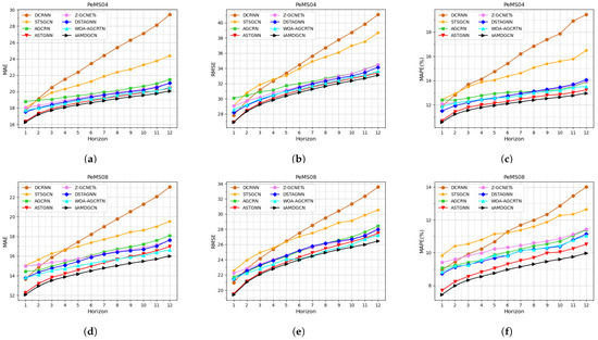
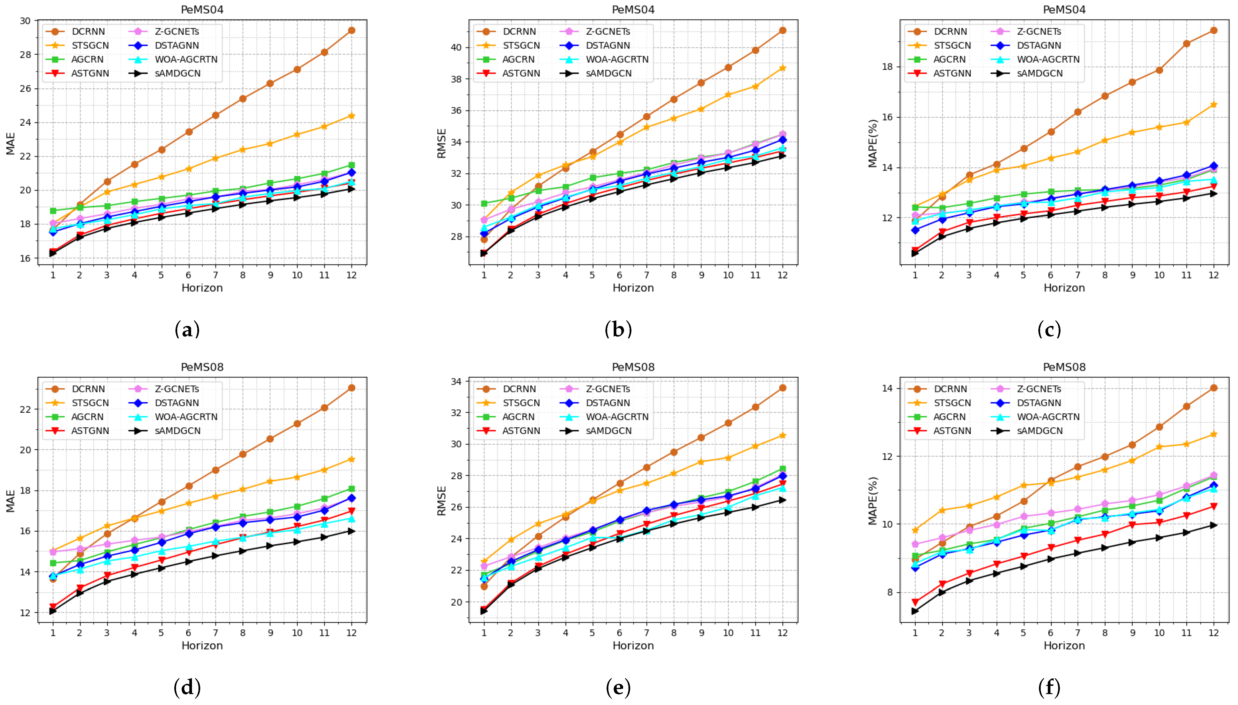
Figure 4.
Performance of sAMDGCN and baseline methods on PeMS04 and PeMS08. (a) MAE on PeMS04. (b) RMSE on PeMS04. (c) MAPE on PeMS04. (d) MAE on PeMS08. (e) RMSE on PeMS08. (f) MAPE on PeMS08.
As can be seen from Figure 4, the prediction errors of all models increase as the time step increases, but the error growth rate of our sAMDGCN model is the smallest and it can maintain a high accuracy for a long time. Among them, DCRNN and STSGCN have good prediction performance in the short term, but have obvious limitations for long-term prediction, especially DCRNN, which is based on RNN, has the largest error. The performance of AGCRN, Z-GCNETs, DSTAGNN, and WOA-AGCRTN is very similar, and they can all maintain a small error in long-term prediction. ASTGNN is the closest model to ours. It shows comparable performance to our sAMDGCN in the short term, but is inferior to sAMDGCN in long-term prediction. This is due to the fact that the sLSTM layer in our encoder pays more attention to recent information and can more accurately analyze future trends.
According to most researches, we define traffic flow prediction for the next 3, 6, and 12 time steps as short-term prediction, medium-term prediction, and long-term prediction, respectively. In order to study the performance of sAMDGCN under different time horizons, we choose several baselines with better performance for comparison under the PeMS04 and PeMS08 datasets. The experimental results are shown in Table 4. We can see that sAMDGCN achieves the best performance whether in short-term prediction, medium-term prediction, or long-term prediction. Although all models cannot avoid the decline in prediction accuracy due to the accumulation of errors as the prediction step increases, our sAMDGCN model has significant improvements than the baseline models, which verifies that our model has stronger anti-interference ability in long-term prediction and slows down the accumulation of errors as the prediction step increases.
Table 4.
The prediction performance of short-term, medium-term, and long-term under PeMS04 and PeMS08 datasets. The best results are marked in bold, and the second-best results are underlined.
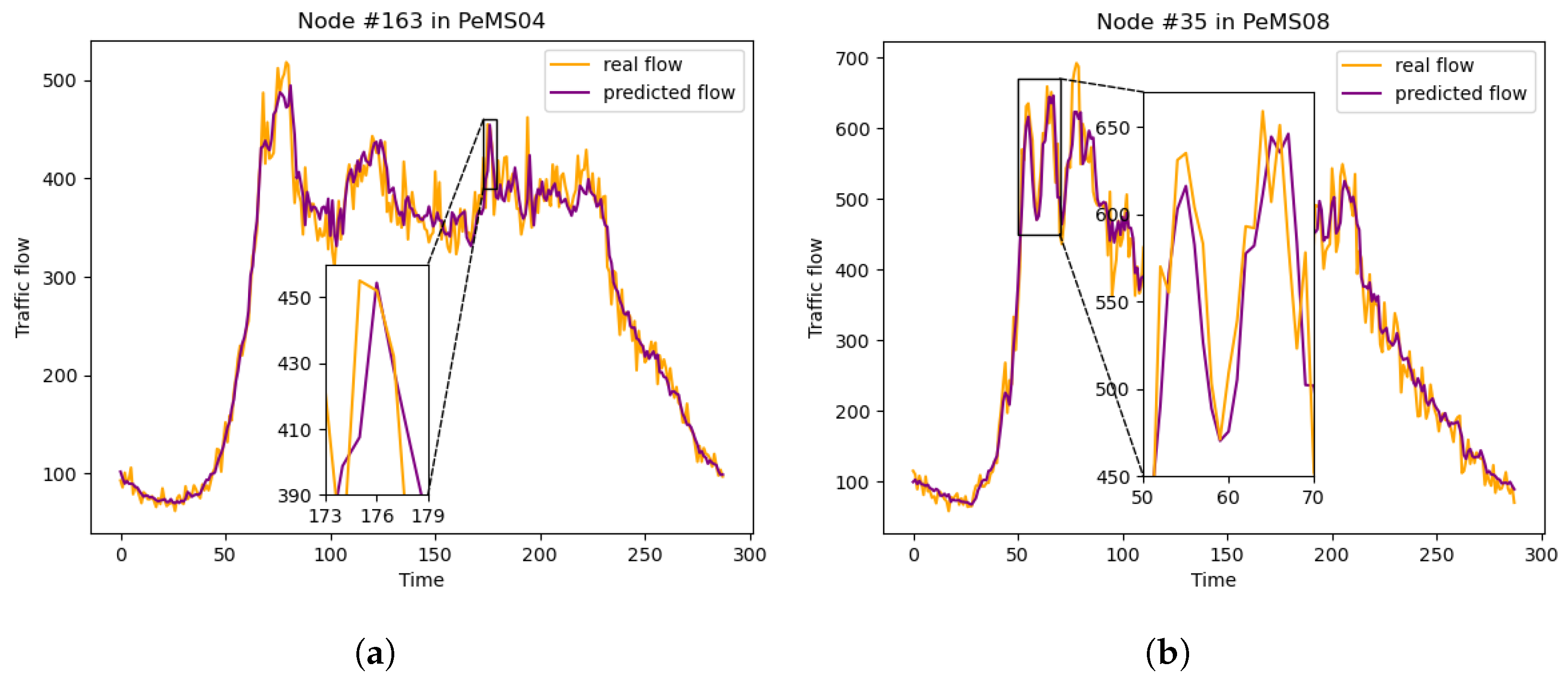
In order to more clearly demonstrate the prediction effect of our model, we randomly selected two nodes, one from PeMS04 and the other from PeMS08, and continuously predict the traffic flow for one day. The predicted values and true values are shown in Figure 5. It is evident that the predicted values closely align with the true values, effectively reflecting the overall trend of traffic flow. Even when there are sudden changes in real traffic flow, our model responds quickly. In summary, sAMDGCN excels because it simultaneously captures both local and global spatiotemporal correlations, making it the most effective model for traffic flow prediction.
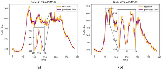
Figure 5.
Comparison results between the prediction values of sAMDGCN and the true values under two nodes during one day. (a) Node #163 in PeMS04. (b) Node #35 in PeMS08.
Further, to evaluate the time cost of our model, we measure the average prediction time of sAMDGCN across four datasets and compare it with ASTGNN, which demonstrates excellent overall performance among the baseline methods. The results are shown in Table 5. These results indicate that sAMDGCN generates predictions swiftly, and it has a very similar prediction time cost compared with the best baseline ASTGNN. Besides, despite the similar prediction time, our sAMDGCN model has higher prediction accuracy than ASTGNN.
Table 5.
The time cost for traffic flow prediction under four datasets.
4.5. Ablation Studies
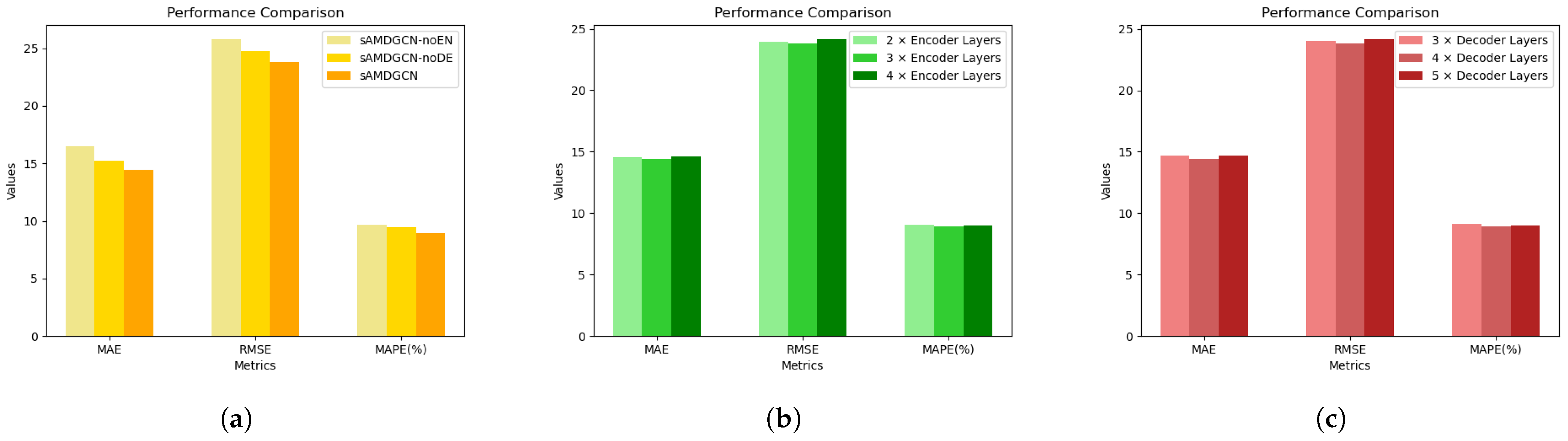
In order to investigate the impact of each component in our sAMDGCN model, we conduct a series of ablation experiments on PeMS08. First, we construct the following two models to study the contribution of the encoder and decoder of sAMDGCN.
sAMDGCN-noEN. Remove the encoder to study the importance of feature extraction of historical sequences. We use the linearly projected historical sequence to replace the output of the encoder in sAMDGCN.
sAMDGCN-noDE. Remove the decoder to study the advantages of generating prediction sequences in an autoregressive manner. We linearly project the output of the last time step in the encoder to generate prediction results for 12 time steps.
Figure 6a shows the comparison results between the above two models and our sAMDGCN. It can be seen that both the encoder and decoder play an important role in our prediction model, and the feature extraction ability of the encoder is the key to the excellent performance of sAMDGCN. Furthermore, we also study the impacts of the number of encoder and decoder layers, and the results are shown in Figure 6b and Figure 6c, respectively.
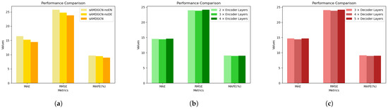
Figure 6.
The impact of encoder and decoder of sAMDGCN. (a) Remove the encoder or decoder. (b) Adjust the number of encoder layers. (c) Adjust the number of decoder layers.
From Figure 6b,c, we can see that compared with the standard sAMDGCN, the performance of the model decreases when the number of encoder layers is less than or more than three. Similarly, the prediction error is minimized when the model has four decoder layers. Therefore, the number of encoder and decoder layers is set to three and four, respectively.
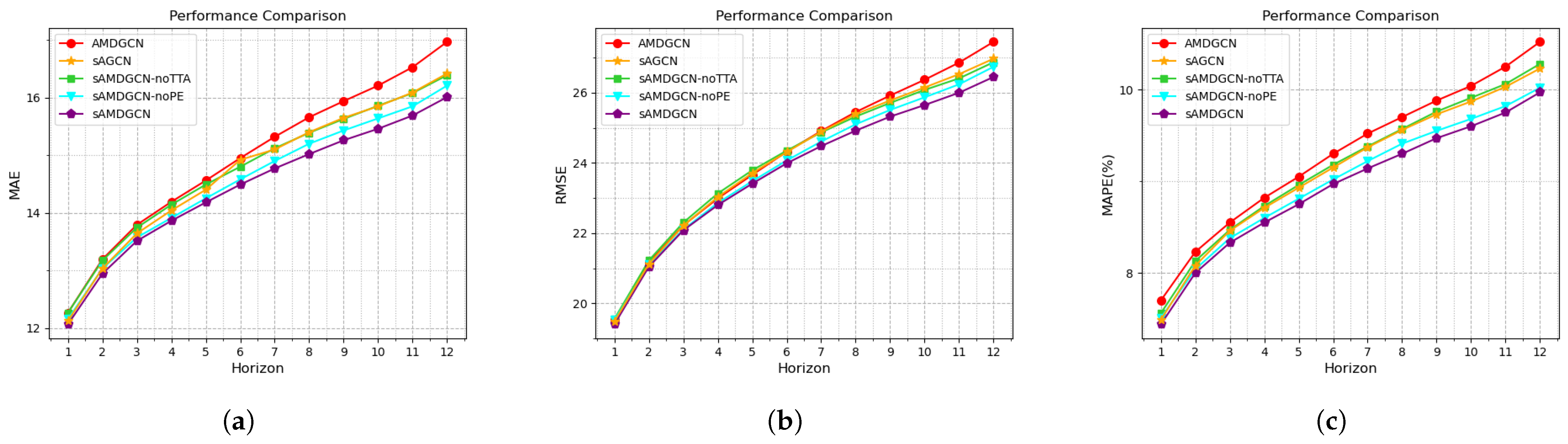
In addition, to also study the role of each module in the encoder and decoder, we design the following four variants.
AMDGCN. The traditional self-attention is used to replace the sLSTM module to study the advantages of the sLSTM module in extracting features.
sAGCN. The traditional GCN is used to replace the MDGCN module to verify the positive effects of the multi-head mechanism and capturing dynamic spatial correlation on traffic flow prediction.
sAMDGCN-noTTA. Linear projection is used to replace the temporal convolution of the attention module in the decoder to verify the importance of temporal trend perception in traffic flow prediction.
sAMDGCN-noPE. Remove the spatiotemporal positional encoding module in the decoder to study the impact of local spatiotemporal information on traffic flow prediction.
The performance of the above four models on PeMS08 is shown in Figure 7. Among them, AMDGCN has the worst performance, which proves that sLSTM has a significant advantage over attention in extracting features. Compared with the standard sAMDGCN, the performances of other models decline to varying degrees, which shows that each module in sAMDGCN has an irreplaceable role.
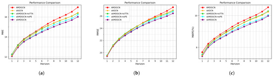
Figure 7.
Performance of AMDGCN, sAGCN, sAMDGCN-noTTA, sAMDGCN-noPE, and standard sAMDGCN on PeMS08. (a) MAE. (b) RMSE. (c) MAPE.
5. Conclusions
In this paper, we proposed a novel sAMDGCN model for traffic flow prediction. sAMDGCN adopted an encoder–decoder structure, introducing sLSTM layers and our newly designed MDGCN module in the encoder to extract the spatiotemporal features of historical data, and using the TTMA module and MDGCN module in the decoder to capture the spatiotemporal dependencies of traffic flow and generate prediction results autoregressively. Experimental results on four datasets verified the effectiveness and robustness of our sAMDGCN model. Compared with baseline methods, sAMDGCN showed high accuracy in long-term prediction. sAMDGCN can not only capture the temporal and spatial correlations hidden in the data but also can effectively respond to sudden changes in traffic patterns. In the future, we plan to incorporate factors like weather changes, unexpected disasters, and unforeseen events like accidents or security threats that can significantly impact the accuracy of traffic flow forecasting models. Moreover, considering optimization strategies and their environmental impact is also crucial and a straightforward research direction.
Author Contributions
Conceptualization, S.Z. and L.H.; methodology, S.Z. and W.K.; software, S.Z.; validation, S.Z. and W.K.; formal analysis, S.Z. and W.K.; investigation, S.Z. and W.K.; resources, H.Q.; data curation, S.Z.; writing—original draft preparation, S.Z. and L.H.; writing—review and editing, S.Z., Y.J., W.K., H.Q., and L.H.; visualization, S.Z.; supervision, H.Q. and L.H.; project administration, H.Q.; funding acquisition, Y.J. and L.H. All authors have read and agreed to the published version of the manuscript.
Funding
This work was partly supported by the National Natural Science Foundation of China under Grant 62306062 and the Independent Project of Intelligent Policing Key Laboratory of Sichuan Province under Grant ZNJW2023ZZZD002.
Data Availability Statement
The data used in this manuscript are publicly available at https://pems.dot.ca.gov/ (accessed on 1 July 2021) and include detailed instructions for using those datasets.
Conflicts of Interest
The authors declare no conflicts of interest.
References
- Ekedebe, N.; Lu, C.; Yu, W. Towards Experimental Evaluation of Intelligent Transportation System Safety and Traffic Efficiency. In Proceedings of the 2015 IEEE International Conference on Communications (ICC), London, UK, 8–12 June 2015; IEEE: Piscataway, NJ, USA, 2015; pp. 3757–3762. [Google Scholar]
- Wei, W.W. Time series analysis. Oxf. Handb. Quant. Methods Psychol. 2013, 2, 458–485. [Google Scholar]
- Williams, B.M.; Hoel, L.A. Modeling and forecasting vehicular traffic flow as a seasonal ARIMA process: Theoretical basis and empirical results. J. Transp. Eng. 2003, 129, 664–672. [Google Scholar] [CrossRef]
- Zivot, E.; Wang, J. Vector Autoregressive Models for Multivariate Time Series. In Modeling Financial Time Series with S-PLUS®; Springer: New York, NY, USA, 2006; pp. 385–429. [Google Scholar]
- Wu, C.H.; Ho, J.M.; Lee, D.T. Travel-time prediction with support vector regression. IEEE Trans. Intell. Transp. Syst. 2004, 5, 276–281. [Google Scholar] [CrossRef]
- Van Lint, J.; Van Hinsbergen, C. Short-term traffic and travel time prediction models. Artif. Intell. Appl. Crit. Transp. Issues 2012, 22, 22–41. [Google Scholar]
- Lipton, Z.C. A Critical Review of Recurrent Neural Networks for Sequence Learning. arXiv 2015, arXiv:1506.00019. [Google Scholar]
- Sutskever, I. Sequence to Sequence Learning with Neural Networks. arXiv 2014, arXiv:1409.3215. [Google Scholar]
- Zhao, Z.; Chen, W.; Wu, X.; Chen, P.C.; Liu, J. LSTM network: A deep learning approach for short-term traffic forecast. IET Intell. Transp. Syst. 2017, 11, 68–75. [Google Scholar] [CrossRef]
- Dai, G.; Ma, C.; Xu, X. Short-term traffic flow prediction method for urban road sections based on space–time analysis and GRU. IEEE Access 2019, 7, 143025–143035. [Google Scholar] [CrossRef]
- Vaswani, A.; Shazeer, N.; Parmar, N.; Uszkoreit, J.; Jones, L.; Gomez, A.N.; Kaiser, L.; Polosukhin, I. Attention is All You Need. In Advances in Neural Information Processing Systems, Proceedings of the 31st Conference on Neural Information Processing Systems (NIPS 2017), Long Beach, CA, USA, 4–9 December 2017; Curran Associates, Inc.: Red Hook, NY, USA, 2017. [Google Scholar]
- Ma, X.; Dai, Z.; He, Z.; Ma, J.; Wang, Y.; Wang, Y. Learning traffic as images: A deep convolutional neural network for large-scale transportation network speed prediction. Sensors 2017, 17, 818. [Google Scholar] [CrossRef]
- Gori, M.; Monfardini, G.; Scarselli, F. A New Model for Learning in Graph Domains. In Proceedings of the 2005 IEEE International Joint Conference on Neural Networks, Montreal, QC, Canada, 31 July–4 August 2005; IEEE: Piscataway, NJ, USA, 2005; Volume 2, pp. 729–734. [Google Scholar]
- Kipf, T.N.; Welling, M. Semi-supervised classification with graph convolutional networks. arXiv 2016, arXiv:1609.02907. [Google Scholar]
- Beck, M.; Pöppel, K.; Spanring, M.; Auer, A.; Prudnikova, O.; Kopp, M.; Klambauer, G.; Brandstetter, J.; Hochreiter, S. xLSTM: Extended Long Short-Term Memory. arXiv 2024, arXiv:2405.04517. [Google Scholar]
- Guo, S.; Lin, Y.; Wan, H.; Li, X.; Cong, G. Learning dynamics and heterogeneity of spatial-temporal graph data for traffic forecasting. IEEE Trans. Knowl. Data Eng. 2021, 34, 5415–5428. [Google Scholar] [CrossRef]
- Wu, Y.; Tan, H. Short-term traffic flow forecasting with spatial-temporal correlation in a hybrid deep learning framework. arXiv 2016, arXiv:1612.01022. [Google Scholar]
- Zhang, C.; Patras, P. Long-Term Mobile Traffic Forecasting Using Deep Spatio-Temporal Neural Networks. In Proceedings of the Eighteenth ACM International Symposium on Mobile Ad Hoc Networking and Computing, Chennai, India, 10–14 July 2017; pp. 231–240. [Google Scholar]
- Yu, B.; Yin, H.; Zhu, Z. Spatio-temporal graph convolutional networks: A deep learning framework for traffic forecasting. arXiv 2017, arXiv:1709.04875. [Google Scholar]
- Wu, Z.; Pan, S.; Long, G.; Jiang, J.; Zhang, C. Graph wavenet for deep spatial-temporal graph modeling. arXiv 2019, arXiv:1906.00121. [Google Scholar]
- Zhao, L.; Song, Y.; Zhang, C.; Liu, Y.; Wang, P.; Lin, T.; Deng, M.; Li, H. T-GCN: A temporal graph convolutional network for traffic prediction. IEEE Trans. Intell. Transp. Syst. 2019, 21, 3848–3858. [Google Scholar] [CrossRef]
- Geng, X.; Li, Y.; Wang, L.; Zhang, L.; Yang, Q.; Ye, J.; Liu, Y. Spatiotemporal Multi-Graph Convolution Network for Ride-Hailing Demand Forecasting. In Proceedings of the AAAI Conference on Artificial Intelligence, Honolulu, HI, USA, 27 January–1 February 2019; Volume 33, pp. 3656–3663. [Google Scholar]
- Bai, L.; Yao, L.; Li, C.; Wang, X.; Wang, C. Adaptive graph convolutional recurrent network for traffic forecasting. Adv. Neural Inf. Process. Syst. 2020, 33, 17804–17815. [Google Scholar]
- Liang, Y.; Zhao, Z.; Sun, L. Dynamic spatiotemporal graph convolutional neural networks for traffic data imputation with complex missing patterns. arXiv 2021, arXiv:2109.08357. [Google Scholar]
- Lee, K.; Rhee, W. DDP-GCN: Multi-graph convolutional network for spatiotemporal traffic forecasting. Transp. Res. Part C Emerg. Technol. 2022, 134, 103466. [Google Scholar] [CrossRef]
- Li, Y.; Yu, R.; Shahabi, C.; Liu, Y. Diffusion convolutional recurrent neural network: Data-driven traffic forecasting. arXiv 2017, arXiv:1707.01926. [Google Scholar]
- Zhao, Z.; Shen, G.; Zhou, J.; Jin, J.; Kong, X. Spatial-temporal hypergraph convolutional network for traffic forecasting. PeerJ Comput. Sci. 2023, 9, e1450. [Google Scholar] [CrossRef] [PubMed]
- Chen, W.; Chen, L.; Xie, Y.; Cao, W.; Gao, Y.; Feng, X. Multi-Range Attentive Bicomponent Graph Convolutional Network for Traffic Forecasting. In Proceedings of the AAAI Conference on Artificial Intelligence, New York, NY, USA, 7–12 February 2020; Volume 34, pp. 3529–3536. [Google Scholar]
- Bai, J.; Zhu, J.; Song, Y.; Zhao, L.; Hou, Z.; Du, R.; Li, H. A3t-gcn: Attention temporal graph convolutional network for traffic forecasting. ISPRS Int. J. Geo-Inf. 2021, 10, 485. [Google Scholar] [CrossRef]
- Xu, M.; Dai, W.; Liu, C.; Gao, X.; Lin, W.; Qi, G.J.; Xiong, H. Spatial-temporal transformer networks for traffic flow forecasting. arXiv 2020, arXiv:2001.02908. [Google Scholar]
- Wang, C.; Wang, L.; Wei, S.; Sun, Y.; Liu, B.; Yan, L. STN-GCN: Spatial and Temporal Normalization Graph Convolutional Neural Networks for Traffic Flow Forecasting. Electronics 2023, 12, 3158. [Google Scholar] [CrossRef]
- Chen, C.; Petty, K.; Skabardonis, A.; Varaiya, P.; Jia, Z. Freeway performance measurement system: Mining loop detector data. Transp. Res. Rec. 2001, 1748, 96–102. [Google Scholar] [CrossRef]
- Song, C.; Lin, Y.; Guo, S.; Wan, H. Spatial-Temporal Synchronous Graph Convolutional Networks: A New Framework for Spatial-Temporal Network Data Forecasting. In Proceedings of the AAAI Conference on Artificial Intelligence, New York, NY, USA, 7–12 February 2020; Volume 34, pp. 914–921. [Google Scholar]
- Chen, Y.; Segovia, I.; Gel, Y.R. Z-GCNETs: Time Zigzags at Graph Convolutional Networks for Time Series Forecasting. In Proceedings of the International Conference on Machine Learning. PMLR, Online, 18–24 July 2021; pp. 1684–1694. [Google Scholar]
- Lan, S.; Ma, Y.; Huang, W.; Wang, W.; Yang, H.; Li, P. Dstagnn: Dynamic Spatial-Temporal Aware Graph Neural Network for Traffic Flow Forecasting. In Proceedings of the International Conference on Machine Learning, Baltimore, MD, USA, 17–23 July 2022; pp. 11906–11917. [Google Scholar]
- Wei, Z.; Zhao, H.; Li, Z.; Bu, X.; Chen, Y.; Zhang, X.; Lv, Y.; Wang, F.Y. STGSA: A novel spatial-temporal graph synchronous aggregation model for traffic prediction. IEEE/CAA J. Autom. Sin. 2023, 10, 226–238. [Google Scholar] [CrossRef]
- Zhang, C.; Wu, Y.; Shen, Y.; Wang, S.; Zhu, X.; Shen, W. Adaptive Graph Convolutional Recurrent Network with Transformer and Whale Optimization Algorithm for Traffic Flow Prediction. Mathematics 2024, 12, 1493. [Google Scholar] [CrossRef]
Disclaimer/Publisher’s Note: The statements, opinions and data contained in all publications are solely those of the individual author(s) and contributor(s) and not of MDPI and/or the editor(s). MDPI and/or the editor(s) disclaim responsibility for any injury to people or property resulting from any ideas, methods, instructions or products referred to in the content. |
© 2025 by the authors. Licensee MDPI, Basel, Switzerland. This article is an open access article distributed under the terms and conditions of the Creative Commons Attribution (CC BY) license (https://creativecommons.org/licenses/by/4.0/).