1. Introduction
The past two decades have witnessed a technological revolution, with numerical methods becoming a cornerstone for advancements across various engineering disciplines, and mechanical engineering is no exception. This progress has been further accelerated by the remarkable evolution of computational power observed since the late 20th century. The availability of increasingly fast, efficient, versatile, and practical computational tools has driven the widespread adoption of advanced numerical methods in engineering simulations [
1]. In particular, its uses have revolutionized the entire mechanical construction industry, allowing for the design of optimized components based on the manufacturer’s imposed constraints, allowing for a close approximated prediction of the component’s behaviour when subjected to real-life working conditions. In the automotive industry, the structural optimization of various parts is a preponderant factor in the vehicle’s components’ performance and behaviour when subjected to stress throughout the driving procedure, demonstrating promising results in weight reduction while maintaining the necessary resistance to ensure that the component fulfils all its mechanical requirements [
2].
In the field of vehicle manufacturing, weight reduction across various components presents an avenue for manufacturers to enhance profitability. Weight reduction often allows for the use of less material per vehicle, further decreasing production costs [
3]. By implementing weight reduction strategies and regular optimization processes on the part-design phase, manufacturers can achieve substantial financial gains through these combined effects. In addition to the financial incentive, growing demand and legislative requirements in the automotive industry have created the need to evolve and develop all types of components involved in the various functional sets of a vehicle so that they are lighter, safer, more efficient in relation to production costs, and, specifically for certain components, more comfortable [
4]. With the need to meet these requirements, the application of structural optimization methods in the automotive field has grown exponentially over the years, keeping with the improvement and evolution of the computational techniques.
The structural evaluation of automotive components is crucial for the development of efficient and safe parts. One way to perform this is through experimental techniques. For example, Liu et al. [
5] developed load spectrum editing for fatigue bench testing, which avoids the need to use the full load spectrum, which could sometimes have minimal impact and significantly increase the testing time. Additionally, computational structural assessment techniques provide engineers with powerful tools to analyse the behaviour of components and systems under various load and stress conditions and complement the overall process of optimization of the studied structure. Through computer simulation, stresses, strains, and displacements can be predicted, allowing the identification of critical failure points to be identified and a efficient optimization of design. For instance, Komurcu et al. [
6] took advantage of numerical techniques to tailor the design of a composite suspension control arm to the required manufacturing considerations.
Weight reduction without compromising the structural integrity of the part can be carried out through structural optimization approaches. The suspension control arm has been the object of study combined with structural optimization techniques; for example, Viqaruddin and Ramana Reddy [
7] designed a suspension control arm with a 30% weight reduction. Also regarding the same component, Llopis-Albert et al. [
8] tested several optimization algorithms to achieve a multiobjective solution for the part. Song et al. [
9] had surrogate models, namely the response surface model and the Kriging model, supporting the stuctural optimization of a suspension control arm and achieved weight reduction between 4.13% and 5.22%. Stiffness optimization is also important in addition to the scope of automotive components. For example, Wang et al. [
10] used a homogenous stiffness domain index to create an optimization model to improve the stiffness of a machining robot. Finally, optimization approaches are not limited to the optimization of stiffness or weight minimization, along with other aspects such as the friction in bearings [
11]. The optimization approach, in this case particle swarm optimization, could also be employed in other applications.
The field of computational mechanics has always been dominated by the use of FEM as the most popular discretization technique in research, development, and education [
12]. However, new techniques have been developed to overcome some of the limitations of the FEM related with its rigid mesh dependency. In areas such as fracture and impact mechanics, areas that approach problems that require meshing due to transient domain boundaries, meshless methods have been shown to be a more accurate alternative to FEM due to not being affected by mesh distortion and not requiring meshing. Unlike FEM, in meshless methods, the nodes are distributed in an arbitrary way, and the field functions are approximated based on a domain of influence, rather than an element. In addition, the rule established in FEM that elements cannot overlap does not apply to the domains of influence of meshless methods: they can and should overlap [
13].
The first meshless method applied in the context of computational mechanics was the DEM (Diffuse Element Method), developed by Nayroles et al. [
14], which used the approximating functions of the Moving Least Squares to construct the approximation functions, a technique previously suggested by Lancaster and S. [
15], Dinis et al. [
16], Poiate et al. [
17]. Later, Belytschko et al. [
18] improved the DEM method and developed one of the most popular and widely used meshless methods: the Element Free Galerkin Method (EFGM). Over time, other methods have also been developed, such as the Petrov–Galerkin Local Meshless Method (MLPG) [
19], the Finite Point Method (FPM) [
20], and the Finite Sphere Method (FSM) [
21].
Although these methods have been successfully employed for a variety of issues in the computational mechanics domain, they all present problems and limitations, one of the main ones being the effect of using approximation functions instead of interpolation functions. The PIM (Point Interpolation Method), developed by Liu and Gu [
22], proved to be a highly attractive approach, as it effectively solves the challenge of imposing essential boundary conditions by constructing shape functions with the Kronecker’s delta property. Furthermore, PIM simplifies the process of obtaining the derivatives of shape functions. Meanwhile, PIM has evolved with the incorporation of radial basis functions for solving partial differential equations [
13,
23]. One of the first truly meshless methods to emerge was the NEM (Natural Element Method) [
24]. Later, new meshless interpolation methods were proposed, such as PIM (Point Interpolation Method) [
22], MFEM (Meshless Finite Element Method) [
25], NREM (Natural Radial Element Method) [
26], and RPIM (Radial-Point Interpolation Method) [
23].
Later, Dinis et al. [
16] introduced the Natural-Neighbour Radial-Point Interpolation Method (NNRPIM), a truly meshless method that leverages the connectivity advantages of the Natural Element Method (NEM) and the interpolation capabilities of the Radial-Point Interpolation Method (RPIM). NNRPIM solely relies the on nodal discretization of the problem domain. It then utilizes this spatial information to autonomously distribute integration points and establish nodal connectivity, eliminating the need for a separate background integration mesh as required by EFGM or RPIM [
16]. This method differs from RPIM as the connectivity between nodes is not described using domains of influence. Instead, it uses influence cells determined by the Voronoï diagram space decomposer [
27] and complemented by the use of Delaunay triangulation [
28]. The Voronoï diagram takes on the task of creating the influence cells from a set of unstructured nodes in the domain. The Delaunay triangulation is applied in order to create a background grid with nodal dependence, which is then used in the integration of the interpolation functions of this method. Thus, when compared with a conventional meshless method, NNRPIM can be considered a truly meshless method, since the set of integration points is totally dependent on the nodal distribution [
13].
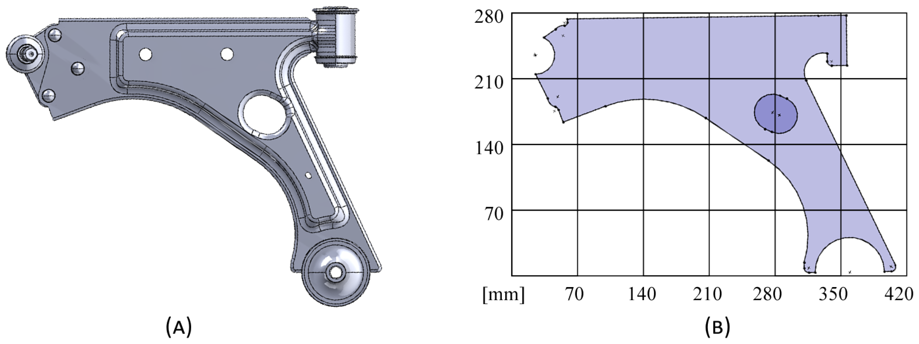
The aim of this study is to utilize a bio-inspired bi-evolutionary optimization algorithm, combined with a natural-neighbour meshless method, for a suspension control arm that has undergone prior accurate modelling and replication. The design of the control arm is based on the geometry of an established industry-standard suspension arm. In automotive mechanical engineering, product development often relies on design philosophies informed by empirical knowledge from engineers. By employing automated techniques to selectively remove material from specific stressed components, it becomes possible to achieve designs that meet manufacturer requirements while significantly reducing mass. Recent literature also highlights a preference for meshless methods, which not only serve as an alternative to FEM but also offer potential advantages [
29,
30]. Being a truly meshless method possesses some advantages. NNRPIM is capable of discretizing the problem domain using only a nodal distribution. All the other mathematical constructions (nodal connectivity, background integration mesh, shape functions, etc.), required to build the system of equations governing the studied phenomenon, are obtained using only the spatial information of the nodes. In the automotive industry, this feature is an advantage since it allows us to obtain the discretization directly from sketches of CAD software (SOLIDWORKS Student Edition 2023 SP2.1) or the output of 3D scanning. Moreover, as the literature shows, NNRPIM shows a high convergence rate and accuracy, which is convenient in structural optimization algorithms depending on the stress field mapping (as the one used in this work). Accurate predictions of the higher and lower stress levels will lead to better remodelling designs.
2. Natural-Neighbour Radial-Point Interpolation Method
Like any other node-dependent numerical discretization method, NNRPIM discretizes the problem domain with a set of nodes, following a regular or irregular distribution. Then, the Voronoï diagram of the nodal set is constructed, using the mathematical concept of the natural neighbours [
31]. For the sake of simplicity, the natural-neighbour procedure will be demonstrated for a 2D Euclidean space, but it can be applied to any n-D space [
13]. Considering the set of nodes
, discretizing the
domain, with
. The Voronoï diagram of
is the partitioning of the spatial domain discretized by
into
. Each sub-region
is associated with a node
so that any point within
is closer to
than to any other node
. The set of Voronoï cells
defines the Voronoï diagram, which is
. The Voronoï cell can be defined by
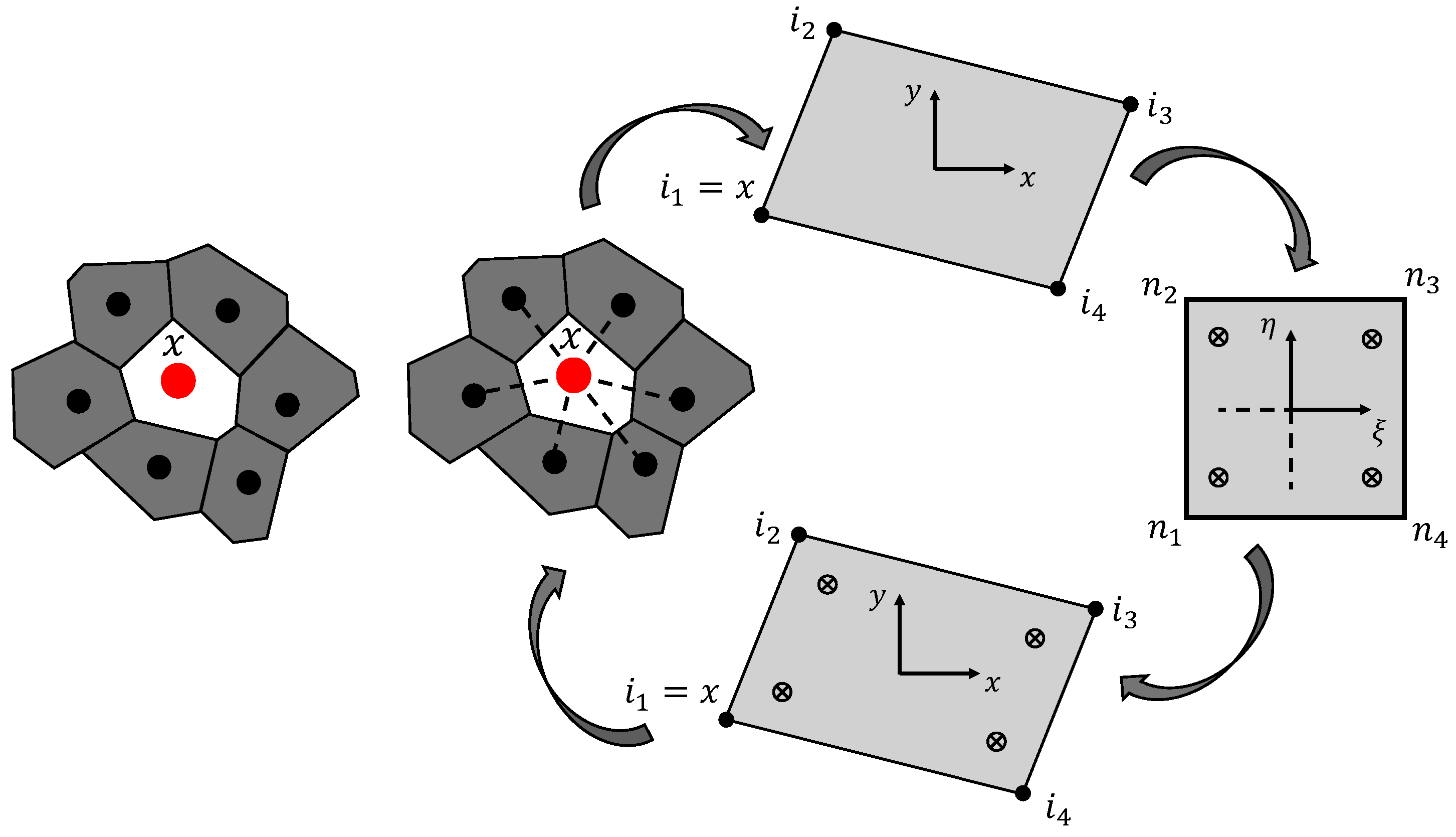
Figure 1 depicts the Voronoï diagram for a general nodal discretization. The natural neighbours of node
are all the nodes whose Voronoï cells share a common edge with the Voronoï cell of node
(represented by the light gray cells surrounding the Voronoï cell of node
in
Figure 1A). The concept of natural neighbours in NNRPIM replaces the need for a pre-defined connectivity information. The Voronoï diagram automatically generates influence domains (called influence cells in the NNRPIM formulation). With this process, it is possible to define a lower-connectivity influence cell and a higher-connectivity influence cell:
First-degree influence cells (
Figure 1A): These comprise node
itself and its immediate natural neighbours. The Voronoï diagram identifies these neighbours as nodes sharing a common edge with the Voronoï cell of
.
Second-degree influence cells (
Figure 1B): These encompass node
, its first-degree neighbours (including natural neighbours of
), and the natural neighbours of those first-degree neighbours.
After the nodal connectivity is established, it is time to build the grid of background integration points. Thus, in order to integrate the integro-differential equation ruling the physical phenomenon, it is necessary to establish the background integration cells. In NNRPIM, the background integration cells are constructed using only the spatial information of the nodal distribution. This is achieved by applying the Delaunay triangulation numerical technique [
13,
28], which is product of the Voronoï diagram of the initial nodal distribution [
13]. Thus, consider a Voronoï cell
of a node
, as in
Figure 2. It is possible to discretize
into smaller quadrilaterals and then apply the Gauss–Legendre quadrature integration scheme to determine the position and weight of integration points within the quadrilaterals. As
Figure 2 shows, NNRPIM employs a two-step process to define such integration points. First, each quadrilateral element in a Voronoï cell is transformed into a unit isoparametric square, which allows for the distribution of the integration points within the isoparametric square in compliance with the Gauss–Legendre integration scheme. Then, the isoparametric coordinates are converted back to the actual Cartesian coordinates of the integration. This process is repeated for each Voronoï cell
discretizing the problem domain. As suggested in the literature, only one integration point is inserted inside each quadrilateral [
13]. Thus, the position of each quadrilateral’s integration point is the quadrilateral’s geometric centre, and its integration weight corresponds to the quadrilateral’s area. A detailed description of the numerical integration procedure of NNRPIM can be found in the literature [
13].
Regarding the connectivity of each integration point, integration points located within the Voronoï cell
inherit the nodal connectivity of node
(i.e., inherit its influence cell). In the NNRPIM, nodal connectivity arises naturally from the overlap of influence cells associated with each integration point. These influence cells define the set of nodes contributing to the shape function construction and stiffness matrix assembly [
13].
The next step is the construction of the shape functions. The NNRPIM uses the radial point interpolators (RPI) technique, which allows the interpolation of the variable field at an integration point
. Thus, consider a function
, defined in the domain
, discretized by a set of nodes
, and assuming that only the nodes included in the influence domain of the point of interest
have an effect on
. The value of the function at the point
can be obtained from the following expression:
in where
represents a radial basis function,
n is the number of nodes inside the influence cell of
, and
and
are non-constant coefficients of
and
, respectively.
Several radial basis functions can be used, and several have been studied and developed over the years. In this work, as recommended in the literature [
13], the multiquadratic radial basis function (MQ-RBF) function will be used [
32]. The MQ-RBF can be described as follows:
for which
is defined as
The variable
is the integration weight of integration point
, and
c and
p are MQ-RBF shape parameters. In the literature, it is possible to find works studying the influence of the MQ-RBF shape parameters on the constructed shape functions [
13]. It was found that assuming
and
leads to shape functions with the delta Kronecker [
13]. Thus, these are the values used in this work. In order to guarantee a unique solution [
23], the following system of equations is added:
Assuming a linear polynomial basis
, with
, it is possible to present Equation (
2) as
solving this system of equations allows us to define the non-constant coefficients
and
,
Inserting
and
into Equation (
2), the following interpolation is obtained:
And, finally, the RPI shape function is defined,
In elasto-static problems, the equilibrium equations governing the partial differential equilibrium can be summarized as: , in which represents the gradient vector, the Cauchy stress tensor, and the body force vector. Regarding the boundary surface, it can be divided into two types: natural boundaries (), where , and essential boundaries (), where . The imposed displacement at the essential boundary is represented as , and the traction force on the natural boundary is defined by (where is a unit vector normal to the natural boundary ).
The Cauchy stress tensor can be represented in Voigt notation,
, as well as the strain tensor,
. Applying Hooke’s law, it is possible to relate the stress state with the strain state,
, being the strain obtained from the displacement field:
. For a generic 3D problem, the differential operator matrix
L and the material constitutive matrix
c can be represented as
where
and
. To establish the system of equations, the virtual work principle is assumed, and energy conservation is imposed:
With the simplification of the above expression, the following can be obtained:
which results in the simplified expression
, where
represents the global stiffness matrix, which can be numerically calculated with:
The
matrix, known as the deformability matrix, can be defined as
With Equation (
12), the body force (
) and external force vectors (
) can also be defined:
where
represents the weight of the integration point on the surface where the external force
is being applied,
is the number of integration points defining the boundary where the force is applied, and
is the interpolation matrix.
The essential boundary conditions are imposed directly on the stiffness matrix
, since RPI shape functions possess the Kronecker delta property. If the problem can be analysed assuming a plane stress simplification, the problem reduces to a 2D analysis, and all components associated with the
direction are removed, thus, reducing the size of all algebraic structures previously presented. For instance, the constitutive matrix and the stress and strain vectors become
and the deformability and interpolation matrices are reduced to
3. Structural Topology Optimization
In computational mechanics, topological optimization is one of the most studied types of optimization due to its ability to generate more efficient and innovative designs. A topological optimization involves the strategic redistribution of material in a structure, resulting in shapes and geometries that are optimized to meet specific criteria, such as strength, stiffness, or other mechanical performance criteria. Assuming a standard topological optimization problem for a given structure, where the aim is to achieve a layout that is as rigid as possible while constraining the structure’s mass, the problem can be formulated by minimizing the average compliance, with the material’s weight constrained. The problem may be described as follows:
where
C represents the average compliance of the structure,
the mass of the selected structure, and
the mass of node
i. The design variable
indicates the presence (
or absence (
of a node in the layout of the defined domain.
Evolutionary computation is a search technique inspired by biological evolution, which uses selection, reproduction and variation to find optimized solutions to complex problems [
33]. In relation to the more conventional optimization techniques, evolutionary techniques are more robust, exploratory and flexible, making them ideal for complex problems with challenging cost functions. Methods such as ESO (Evolutionary Structural Optimization), developed by Xie and Steven [
34], have been widely applied to structural optimization problems in recent years [
34]. The technique is based on the removal of material from a specific domain through an iterative process, material that is considered inefficient and redundant, in order to obtain a design that is considered optimal [
35]. Despite the widespread use of the ESO method, this method presents problems and limitations that have led to the necessity of investigating new techniques. In order to improve the viability of the solutions obtained in the optimization, the need to create a bidirectional algorithm appears, which would allow not only the removal of material in order to eliminate areas that demonstrated low stress but also the addition of material to compensate for areas of high stress. This led to the creation of the bidirectional evolutionary structural optimization method, or BESO (Bi-Directional Evolutionary Structural Optimization), a method inspired not only by the material removal capabilities of ESO but also by the additive material capabilities of AESO [
36], an additive evolutionary structural optimization method (Addition Evolutionary Structural Optimization), which allows for a more careful search of the design domain while also offering a superior ability to find the global minimum [
37].
An elasto-static analysis step initiates each optimization iteration, returning the displacement, strain, and stress fields. As such, it is possible to calculate the equivalent von Mises stress for each integration point, as well as the cubic average of the von Mises stress field, which serves as a reference to help detecti sudden stress changes. With a high value of stress, the cubic average is highly affected. Meanwhile, with low values of stress, the average is practically unaltered.
Next, a penalty system is applied in order to describe and attribute a specific parameter, in this specific case the density, to each integration point. In this work, the interval values for the penalty are assumed to be , where 1 represents the rewarded domains, or solid material, and the penalized domain, or removed material. The BESO procedure performance depends on the reward ratio, , and the penalization ratio, . The integration points with the highest and the integration points with the lowest are identified. The points are rewarded with , while the points are penalized with . Each node is then assigned a penalty parameter . For each integration point , the closest nodes update their penalty values with . After updating all nodes, the penalty parameters for each integration point are recalculated in order to filter and smooth the selected penalty parameters using the interpolation function , where n is the number of nodes inside the analyzed influence domain of , and is the shape function vector of the integration point . At the end of the first iteration, some values differ from one, indicating the absence of material. The process can then proceed to the next iteration. In iteration j, the penalty parameters will be used to modify the material constitutive matrix. Consequently, the penalized constitutive material matrix is calculated. In the following iteration j, the stiffness matrix is calculated, using instead of . The same steps follow, and a new equivalent von Mises stress field is obtained. Through it, the new cubic average stress is calculated, and the comparison is made. If the condition is true, the integration points with are rewarded with . The penalty parameters are recalculated, updating the material domain for the next iteration .
The structural optimization algorithm used in the present work is a BESO - inspired algorithm, developed for applications in the biomechanics field, namely bone-remodelling applications. In a relation known as Wolff’s law, bone tissue directionality increases its stiffness in response to external applied loads [
38]. In order to predict this behaviour, several researchers have developed laws based on observations and experimental tests able to predict bone behaviour based on the different load cases considered. The created models are the basis for computational bone analysis, and the model used affects the results of the simulations carried out. Various models have been established, ranging from the Pauwels’ model [
39] to other models with extra considerations or different approaches to the problem, such as the Corwin’s [
40] and Carter’s [
41].
Carter’s model is identical to Pauwels’ model in that it requires a mechanical stimulus for remodelling to occur. This stimulus is calculated based on the effective stress, which takes into account both the local stress and the bone density, as well as the number of load cycles to which the bone is subjected (represented by the exponent
k). The higher the magnitude of stress, the stronger the stimulus for remodelling.
The model assumes that the applied stress acts as a built-in optimization tool. The goal is to achieve a balance between maximizing the structural integrity of the bone (strength) and minimizing its mass. This can be achieved by minimizing an objective function that mathematically represents this goal.
The model also offers the option of using stress or strain energy as the basis for optimization. Strain energy focuses on maximizing the bone’s stiffness (resistance to bending), while stress focuses on optimizing the material’s strength. By using strain energy, the model relates the apparent density of the bone to the local strain energy it experiences. This makes it possible to estimate the bone’s density at the remodelling equilibrium, a state in which bone resorption and formation are balanced.
If the bone is under stress from several directions, the model combines the effects of each stress pattern in a single direction. This direction is referred to as the normal vector (
) and represents the ideal alignment for the bone’s internal support structures (trabeculae) for optimum strength. To calculate this ideal direction, the model considers the normal stress acting on the entire bone, which is specified in Equation (
27).
The algorithm, originally developed for this work, was incorporated in the previous codes already programmed by the research team, which included a bone-remodelling model adapted for meshless methods developed by Belinha et al. [
42]. This new approach assumes that a mechanical stimulus, adequately represented by stress and potentially strain metrics, serves as the key factor influencing the bone-tissue-remodelling process. A detailed description of the entire model can be found in the literature [
13]. Through the described bone-remodelling procedure, the remodelling itself functions as a topological optimization algorithm. Thus, in each iteration, only the points with high/low values of energy deformation density optimize the density based on its mechanical stimulus. A detailed description of the procedure can be found in the literature [
13].
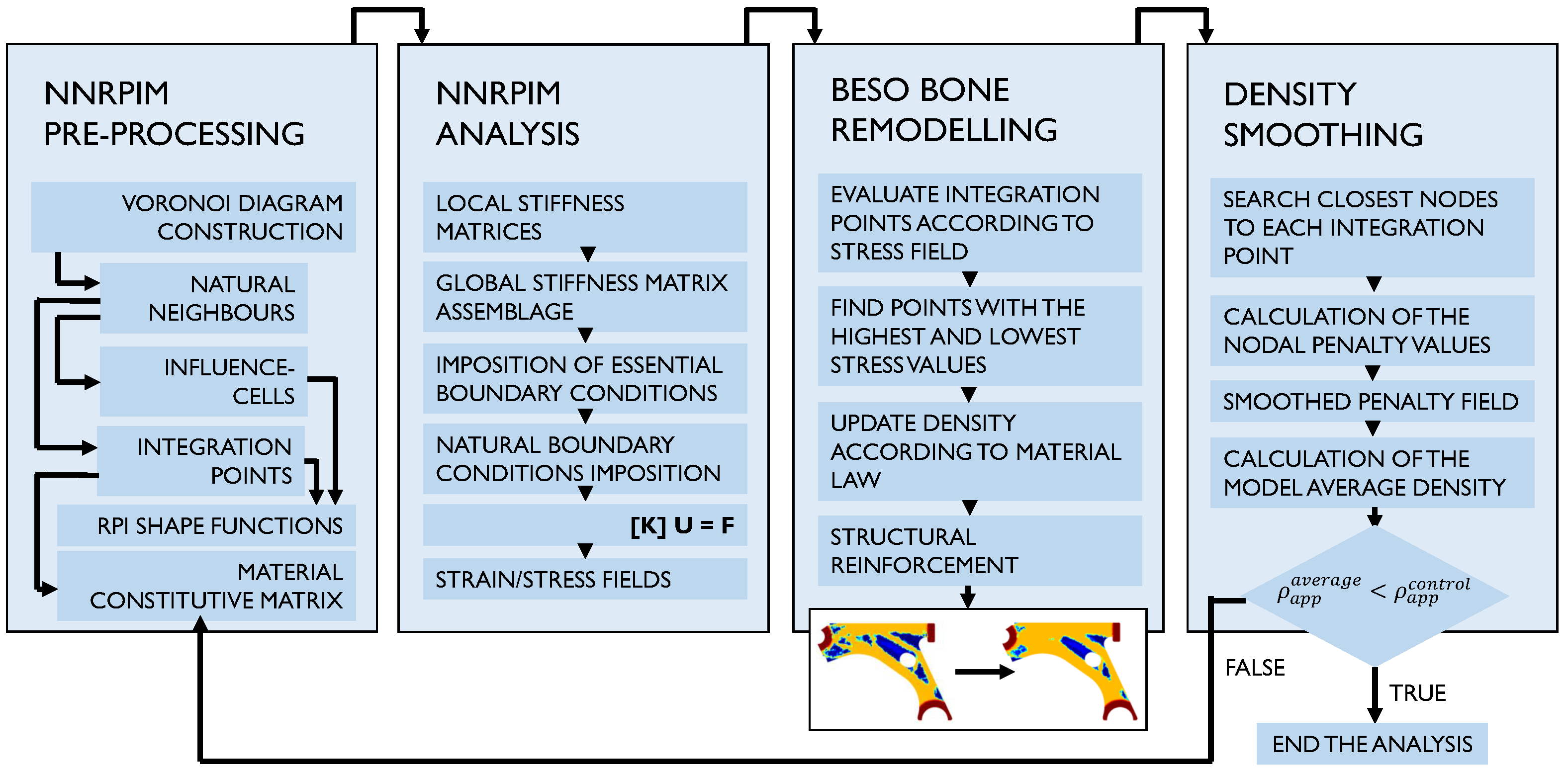
Figure 3 presents a scheme of how the optimization topology algorithm inspired by the bone-remodelling flowchart would present the NNRPIM method. As the flowchart shows, the structural optimization algorithm applied in this work is iterative. Thus, in each iteration, for a given material distribution, the stiffness matrix is calculated and the variable fields are obtained (displacements, strains, and stresses). Then, the
integration points with lower stress levels have their material density reduced, which will reduce their mechanical properties (notice that
is the total number of integration points and
is the penalization ratio, established in the beginning of the analysis). A similar procedure occurs for the
integration points a with a higher stress level; their material density will increase, which will increase their mechanical properties (where
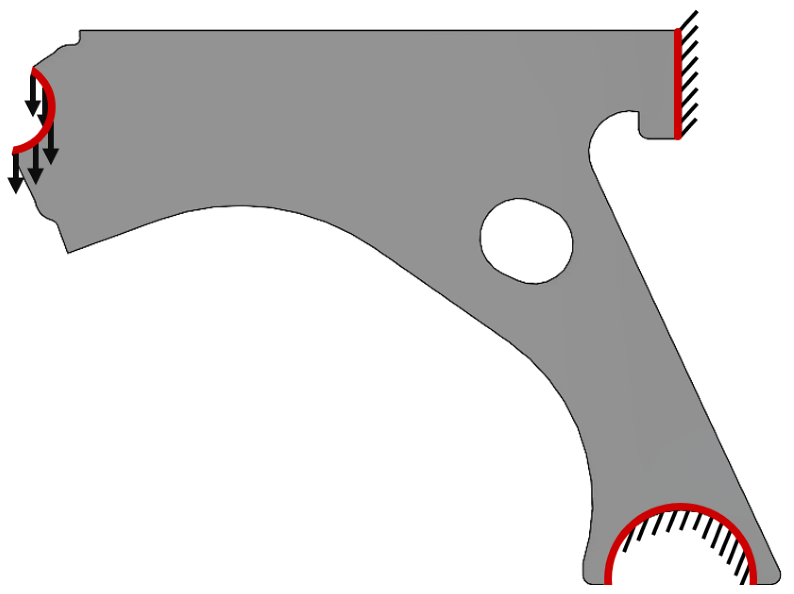
is the reward ratio, established at the beginning of the analysis). Then, in the next iteration, the material distribution changes, leading to new variable fields and a consequent new remodelling scenario. The remodelling process ends when the average density of the model is lower than a threshold valued initially defined by the user. Since the FEM and NNRPIM formulations are different (from a mathematical point of view), for the same material model, they lead to different variable fields (very close, but different). Because the adopted optimization algorithm is iterative, and since the solution of the next iteration is dependent on the solution of the previous iteration, it is not straightforward that the FEM and NNRPIM analyses tend to the same solution.
5. Conclusions
The focus of this work was the application of the NNRPIM, combined with a bi-evolutionary topological optimization algorithm, for the analysis of a standard automotive mechanical component. In parallel, a well-known FEM formulation was also used for comparison purposes. The analysed mechanical component was a standard suspension control arm, in which the 3D CAD was converted to a simplified two-dimensional layout in order to streamline and minimize the computational cost of the numerical simulations conducted.
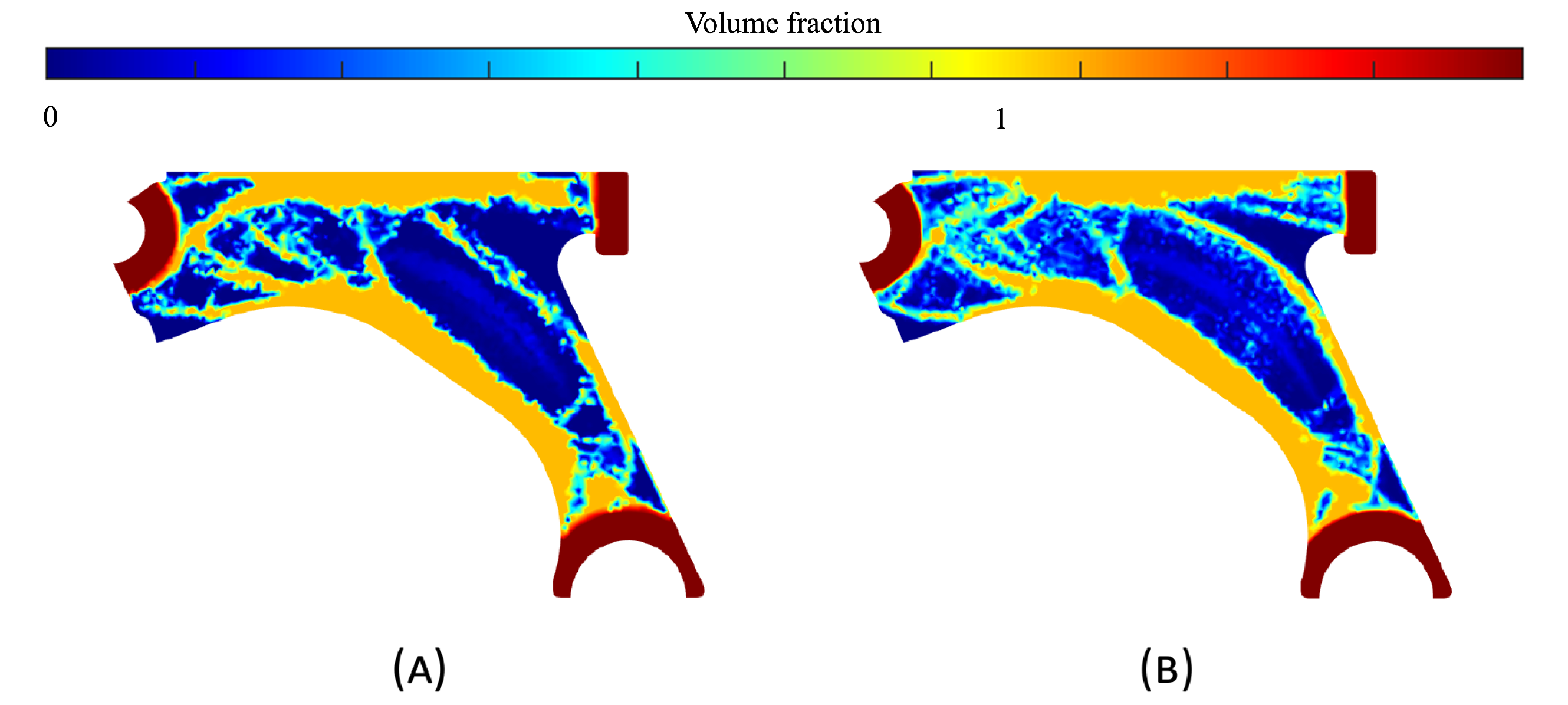
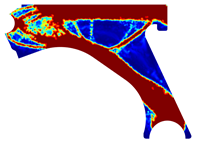
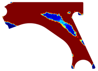
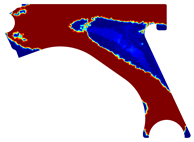
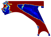
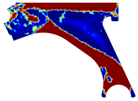
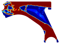
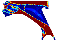
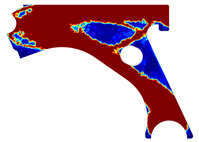
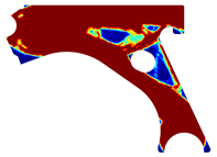
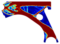
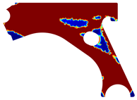
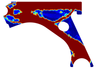
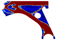
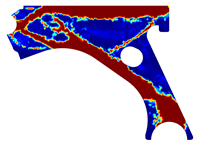
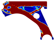
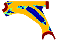
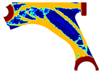
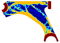
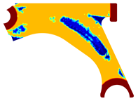
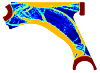
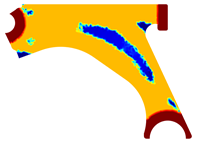
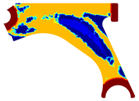
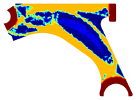
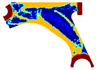
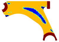
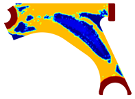
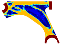
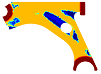
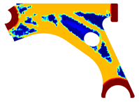
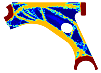
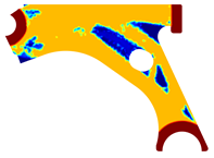
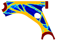
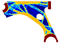
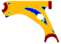
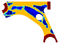
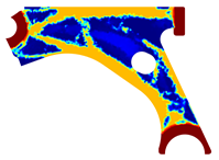
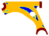
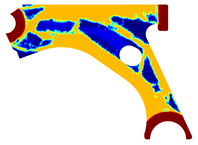
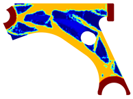
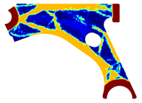
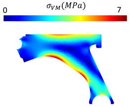
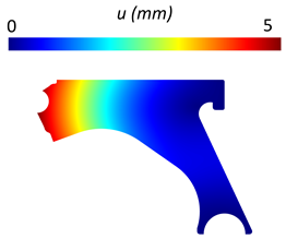
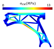
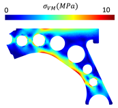
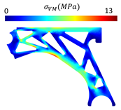
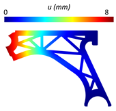
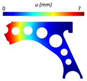
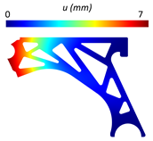
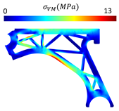
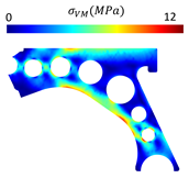
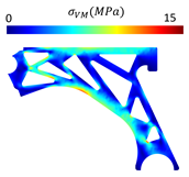
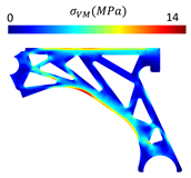
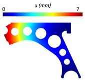
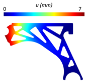
When assessing the obtained solutions, it was noticeable that NNRPIM generated topologies with better truss connection and a higher number of intermediate densities (intricate bone-like trabecular distributions), features that would greatly benefit the mechanical performance of an hypothetical part manufactured by means of additive manufacturing. Subsequently, four designs were built based on a solution obtained from the previously mentioned algorithm, following material-removal approaches commonly applied in the automotive industry for the studied component: a model with a trussed design, a model with circular material removal, a model with triangular material removal, and a model equivalent to the previously mentioned, albeit with an increase in the boundary contour thickness to 1.5 times the nominal thickness of the remaining model. By means of an linear static analysis in the same conditions applied to the optimization algorithm, it was observable that the design based on circular material removal demonstrated the best stiffness and specific stiffness, proving the original hypothesis, since the circular shape allows for a more uniform distribution of stresses in the structure. This kind of solution is recurrent in the automotive industry, and the results presented show that this simple solution is efficient and practical. The trussed and triangular models exhibited similar behaviour, as the principle for their material removal is similar. Model 4 (reinforced at the contour), as expected, displayed a lower displacement, and consequently a higher stiffness, compared to model 3. However, as a result, its increase in mass and total volume led to a negligible difference in specific stiffness between models 3 and 4. There were minor discrepancies observed in the von Mises stress fields and maximum stress values obtained with FEM and NNRPIM. Similarly, small differences were observed in the displacement values, which can be attributed to the higher rigidity of triangular elements.
Regarding the relative difference between both formulations, the obtained results show that concerning the displacement, NNRPIM is able to produce results very close to FEM. For instance, for model 1, the relative difference is , and for all the other models, the relative difference ranges between and . Regarding the maximum von Mises stress, the results show that the relative differences obtained for the solid model and model 1 are and , respectively, which are very close. However, for models 2, 3 and 4, the relative difference increases, ranging from and , indicating that some stress-concentration zones produce distinct von Mises stress values. The directional stiffness of both formulations is very close, ranging between and . These results reinforce the idea that NNRPIM is a valid numerical alternative to the FEM.
In other applications associated with remodelling and BESO algorithms, NNRPIM already proved to be efficient, delivering optimal solutions for automotive parts, such as wheels and brake pedals [
44], or the development of new optimized functional materials [
47] and their cellular foam structure [
48]. In this work, it was shown again that NNRPIM is able to produce results with satisfactory similarity to FEM, indicating that it could represent a viable alternative to FEM topological optimization analyses. Future research directions on this topic will include the extension of the application to 3D analyses in order to include out-of-plane forces and torsion effects; the inclusion of functionally foam material (to fill the voids and reduce stress concentration phenomena) and its prototype production and experimental validation using 3D printing techniques; and the inclusion of artificial neural networks to surrogate the FEM/NNRPIM processing block, allowing for much faster computational analysis [
49].

