Abstract
In the context of team collaborative tasks, continuous operational capability represents a crucial indicator of operational efficiency and a pivotal area of current research. A reduction in the continuous operational capability of team members will inevitably result in an increase in the error rate, which will prevent the completion of the task. In certain circumstances, this may even result in more severe consequences. To guarantee that team members possess optimal operational capabilities, it is imperative to conduct research on continuous operational capability prediction. This paper presents a Bayesian network-based continuous operational capability prediction model for team collaborative tasks. The model is developed based on the causal relationship of the continuous operational capability evolution, and through the improvement on the Bayesian network so that it can be suitable for individual personnel. The experimental verification demonstrates that the model produces accurate results and can be employed to predict the continuous operational capability and its changing trend.
Keywords:
Bayesian network; team collaborative task; continuous operational capability; prediction model MSC:
62C10
1. Introduction
To guarantee a high-quality output in the context of the team collaborative task, it is essential to gain insight into the operational status of the team members. This necessitates the ability to predict and analyze their continuous operational capabilities. The factors closely related to the continuous operational capabilities of team members generally include the working environment and various aspects such as the operational capabilities, cognitive abilities, psychological states, and physical states of the members. Team members operate in this environment with restricted activities for an extended period, which ultimately results in a decline in their abilities across some domains. This is usually evidenced by a reduction in operational capability, deterioration in cognitive ability, emergence of abnormal bioelectric signals, and an increased proclivity for the development of psychological disorders and negative emotional states. Extended periods of high-stress teamwork have been identified as a potential risk factor for reduced work efficiency and an increased risk of mission failure. In severe cases, this may also have implications for personnel safety [1,2,3]. A comparable phenomenon can be observed in everyday driving. After the driver has maintained a high level of concentration for an extended period in a constrained environment, their response time slows down, increasing the risk of an accident. Fatigue-related driving has emerged as a significant contributing factor to traffic accidents in certain countries [4,5]. It is thus imperative to develop a methodology that can accurately predict and assess the continuous operational capability of team members. Although scholars have conducted research on the operational capability evolution based on various characteristic indicators and methods, there are still shortcomings in the existing methods. For instance, the causal mechanism of the operational capability evolution is not clear, and the characteristics of individual personnel themselves are not taken into account. Hence, it is necessary to build a continuous operational capability prediction model for team collaboration task operators with these problems settled. This will be elaborated in detail in the following text.
The application of prediction and analysis methods to the continuous operational capability in existing research typically entails the observation and measurement of several characteristic indicators of operators in real time. Subsequently, the data is subjected to an evaluation process employing suitable analytical techniques, thereby enabling the operator’s work status to be ascertained with a reasonable degree of accuracy. One potential approach to forecasting an operator’s continuous operational capability is to conduct an analysis with a focus on the operator’s specific characteristics, including physiological and behavioral characteristics [6,7,8]. To illustrate, Mansikka et al. [9] examined the heart rate and heart rate variability of pilots during instrument flight rules (IFRs) proficiency tests. Their findings suggest that these physiological indicators can be employed to assess the mental load experienced by pilots, thereby providing a theoretical foundation for analyzing the evolution of continuous operational capability through physiological indicators. In a recent study, Lu et al. [10] investigated the efficacy of utilizing a consumer-grade wearable device to monitor heart rate variability in order to detect driver sleepiness under both manual and partially automated driving conditions. Their findings demonstrated that this method can be employed to effectively monitor driver sleepiness. In addition to these studies based on physiological characteristics, scholars have also developed prediction models for personnel continuous operational capability based on human behavioral characteristics. To illustrate, Lopez et al. [11] proposed an exercise-induced fatigue detection method based on thermal imaging technology. This method is based on the changes in facial features that occur during the fatigue state and can detect exercise-induced fatigue without interfering with their normal work activities by detecting facial characteristics. Quddus et al. [12] put forth a methodology for detecting indications of human fatigue through the observation of eye movement behaviors, predicated on the changes in eye movement in conjunction with the onset of fatigue. Additionally, He et al. [13] developed and validated a sleepiness detection system based on eye activity sensors for the purpose of identifying whether drivers are in a fatigued state. The system employs sensors to capture the blinking frequency of the driver and utilizes analytical and processing techniques to recognize the fatigued state. Although these studies provide important references for predicting continuous operational capability, they still have significant limitations, including the inability to quantify fatigue status and the difficulty of providing accurate analysis results based solely on a single characteristic indicator.
It is precisely because these techniques for forecasting continuous operational capability based on a single indicator are inadequate in terms of both comprehensiveness and accuracy that scholars have put forth additional prediction methods for continuous operational capability. These methods encompass a range of approaches, such as approaches integrating multiple indicators of the same type and approaches integrating indicators of different types. For example, in a study by Lees et al. [14], the effects of a monotonous driving task (MDT) on the cardiac health of train drivers were investigated. The findings revealed a coupled relationship between electroencephalogram (EEG) activity and heart rate variability parameters, providing a new perspective for analyzing operational capability by combining multiple characteristic indicators. In a recent study, Markus et al. [15] developed a driver fatigue monitoring system that employs low-cost electrocardiogram (ECG) sensors to calculate personnel heart rate variability data, which is then used to predict fatigue states. Additionally, the system incorporates facial recognition technology to enhance the accuracy of driver fatigue monitoring in situations where lighting is poor, or the driver is partially or fully obscured. Wu et al. [16] developed a method for recognizing and determining the fatigue level of drivers based on EEG signals, eye movement features, and ECG signals. They also innovatively applied a Cere-bella Model Articulation Controller (CMAC) neural network for fatigue state recognition. Nevertheless, there are still problems with these studies, including unclear causal analysis of the operational capability reflected in the models. In addition, the majority of prediction models of continuous operational capability developed by extant studies are generalizable for various operators, yet there is a paucity of modeling studies that are applicable to individual personnel.
Due to the numerous problems with the existing studies mentioned previously, in order to ensure the work efficiency of team collaboration task operators, it is crucial to construct a prediction model for continuous operational capability that comprehensively considers the causal relationship of continuous operational capability evolution and individual personnel characteristics. This paper presents a methodology for predicting the continuous operational capability of team members. It addresses the wide range of factors affecting the evolution of continuous operational capability and the need to apply this methodology to the study on individual personnel. As previously indicated, the continuous operational capability predictive model developed in this study is based on the underlying causes and consequences of continuous operational capability evolution. Consequently, the Bayesian network method is an appropriate mathematical approach to employ. A Bayesian network is a model that enables the inference through cause-and-effect relationships [17,18]. The utilization of a Bayesian network to construct a continuous operational capability evolution model is an exercise in probabilistic reasoning that commences with an examination of the underlying cause and effect of the continuous operational capability change. In this paper, a prediction model for the evolution of continuous operational capability applicable to individual operators in the team has been constructed on the basis of the causes and consequences of continuous operational capability evolution, using a prediction model based on dynamic Bayesian networks. Concurrently, a number of researchers were invited to conduct experiments on the evolution of continuous operational capability. The objective was to analyze the trend of continuous operational capability evolution and to verify the accuracy of the prediction results of this model.
2. Methods
2.1. Predictive Principle of Continuous Operational Capability
2.1.1. Causal Analysis of the Evolution of Continuous Operational Capability
In order to construct a model for the continuous operational capability evolution of team members, it is first necessary to analyze the environment–human–task characteristics of the special operating environment of the particular teamwork. On this basis, the causes and results of the continuous operational capability evolution of team members are analyzed referring to the consultation with experts in the same research field as this paper, and an index system for evaluating the risk of continuous operational capability fluctuations is constructed; this reflects the causes of the continuous operational capability evolution, as well as an index system for observing and evaluating the evolution of continuous operational capability, which reflects the results of the continuous operational capability evolution.
Based on the analysis of the environment–human–task characteristics of the teamwork operating environment, this paper determines factors that need to be considered for the analysis of continuous operational capability evolution.
- Working environment
The working environment of the particular teamwork is somewhat isolated from the natural environment and requires special control. Consequently, there are certain differences between it and ordinary working environments in terms of various factors, including illumination, noise, gas concentration, temperature, and humidity. The impact of these factors on human health differs from that of ordinary working environments [19,20,21,22]. Therefore, this paper considers the working environment in the construction of the continuous operational capability evolution model.
- 2.
- Task load
In the team collaborative work environment, the primary objective for operators is to successfully complete their tasks. The purpose of carrying out various supporting measures is to provide the necessary resources and assistance to operators, enabling them to excel at their tasks. Given the considerable demands placed on operators to respond swiftly and accurately, task load is identified as a pivotal factor influencing the evolution of continuous operational capability [23]. The primary considerations are the current workload and the accumulated workload during the day.
- 3.
- Learning and assistance of task
The continuous working capability of the operator may be affected by the learning of tasks. The deployment of intelligent assistance technology during tasks provides operators with varying degrees of assistance, which in turn affects their continuous working capability [24]. Accordingly, this paper incorporates the learning and assistance of task into the construction of the continuous working capability evolution model, encompassing task anticipation capability and task intelligent assistance level.
- 4.
- Working time
In light of the fact that the operating hours of the particular team collaborative task encompass all time periods of the day, it is imperative to consider the role of operating time factors in this article. These factors primarily encompass the impact of operating time periods, that is, the operating time domain and the cumulative operating time during the day; they also encompass the impact of resting time, that is, the resting time since the last operation and the cumulative resting time during the day [25,26].
Concurrently, this article identifies the following results that must be considered in the analysis of continuous operational capability evolution:
- Perceptual–comprehensive–predictive capability
The perceptual, comprehensive and predictive capabilities of team members directly correlate with the proficiency of the operator in executing tasks [27,28,29]. When team members perform tasks in an optimal manner, these three abilities are typically observed to be robust. Members are able to identify the type of task in a timely manner, comprehend the operations that need to be performed, anticipate the trajectory of the task, and demonstrate a relatively short response time and a relatively high accuracy when tested on these abilities. This paper considers these capabilities as the result of the continuous operational capability evolution. The main indicators of this capability are the response time (RT) and accuracy rate (ACC) of the tasks.
- 2.
- Decision-making capability
When team members have completed their assigned tasks in an exemplary manner, they frequently demonstrate robust decision-making abilities [30]. Members are able to make rapid and precise decisions in accordance with the circumstances at hand. Similarly, the decision-making ability test exhibits a relatively short response time and a relatively high accuracy rate. This paper considers decision-making capability as the result of the continuous operational capability evolution.
- 3.
- Cognitive capability
Cognitive capability is a crucial capacity for team members to perceive alterations in the surrounding environment and obtain tasks while undertaking tasks [31,32]. It encompasses attention vigilance, attention, working memory, implicit emotions, and other factors, and serves as an indicator of the continuous operational capability evolution.
- 4.
- Psychological state
Given that psychological state indicators reflect the psychological and emotional state of team members, it can be surmised that this state may reflect the quality of the team members’ working state and, in turn, their continuous operational capability [33]. This paper considers the role of psychological state in the evolution of continuous operational capability, with a particular focus on the concepts of alertness and task satisfaction.
- 5.
- Physiological state
Physiological state indicators represent a crucial set of parameters that reflect the physiological state of team members. They can serve as a foundation for elucidating the evolution of continuous operational capability [12,15,34]. This paper considers the role of physiological state in the study of the evolution of continuous operational capability, with a particular focus on eye movement signals, ECG signals, rhythm interference, and body fatigue.
In light of the aforementioned analysis of causes and results, a causal link diagram illustrating the evolution of continuous operational capability is presented in Figure 1.
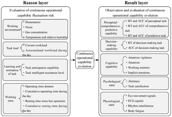
Figure 1.
Casual relationship of continuous operational capability evolution.
2.1.2. Quantification and Normalization of Reason and Result Indicators of the Continuous Operational Capability Evolution
The above causal analysis of the of continuous operational capability evolution unambiguously identifies the four types of cause indicators and five types of result indicators, which are the basis of the continuous operational capability prediction model established in this paper. In order to further establish a basis for the quantitative analysis of the continuous operational capability evolution to complete the construction of the model, this paper provides the quantitative methods for the aforementioned reason indicators and result indicators. Therefore, indicators with different measurement methods and units can be quantified based on the same standards. The methodology for quantifying and normalizing these indicators is to utilize a scale of no less than 0 and no greater than 1, whereby a value of 1 represents the optimal condition for continuous operational capability and a value of 0 signifies the least favorable condition for continuous operation capability. In accordance with the aforementioned methodology, the quantitative and normalization method for establishing the four types of reason indicators is as follows:
- Working environment
Previous research has identified the impact of environmental factors, including illumination, noise and gas concentration, on working ability [35,36,37,38]. These factors have been quantified as c11, c12 and c13, respectively. The temperature and humidity indicators are quantified as c14 in accordance with the conventional PMV calculation methodology [39]. These quantified results are averaged with equal weight and serve as the quantified result c1 for the working environment.
- 2.
- Task load
The distribution of tasks in the timeline is recorded, and the timeline analysis method [40] is employed to quantify the task load. The current workload is quantified as c21. Representing the current workload accumulated over the course of the day, the accumulated load during the day is calculated as c22. These quantified results are averaged with equal weight and serve as the quantified result c2 for the task load.
- 3.
- Learning and assistance of task
The task anticipation capability is quantified as c31 by analyzing the learning success rate of team members. According to the OODA theory [41,42], a quantitative value, designated c32, is assigned to the task intelligent assistance level through the analysis of observation, judgment, and decision-making. These quantified results are averaged with equal weight and serve as the quantified result c3 for the learning and assistance of task.
- 4.
- Working time
Based on the analysis of the impact of working hours according to existing studies [25], the quantitative results c41 and c42, which represent the operating time domain and the cumulative operating time during the day, respectively, are presented. Based on the results of the performance degradation risk index calculation [26], the quantitative results of the resting time since last operation and the cumulative resting time during the day are designated as c43 and c44, respectively. These quantified results are averaged with equal weight and serve as the quantified result c4 for the working time.
Similarly, the quantitative and normalization methods for the five types of result indicators are established as follows:
- Perceptual–comprehensive–predictive capability
Perceptual capability is characterized by the response time and accuracy rate for perceptual tasks, quantified as g11 and g12, respectively. Similarly, comprehensive capability is defined by the response time and accuracy rate of comprehensive tasks, which are quantified by g13 and g14, respectively. Predictive capability is defined by two key factors: the response time and accuracy rate of the predictive task. These are quantified by g15 and g16, respectively. These quantified results are averaged with equal weight and serve as the quantified result g1 for the perceptual–comprehensive–predictive capability.
- 2.
- Decision-making capability
The decision-making capacity is defined by the response time and accuracy rate of the decision-making task, which are quantified as g21 and g22, respectively. These quantified results are averaged with equal weight and serve as the quantified result g2 for the decision-making capability.
- 3.
- Cognitive capability
The degree of attention vigilance is determined by the response time and accuracy rate of the PVT test [43,44], which are quantified as g31 and g32, respectively. The attention is determined by the response time and accuracy rate of the Stroop test [45,46], which are quantified as g33 and g34, respectively. The working memory is determined by the response time and accuracy rate of the GO-NOGO test [47,48], which are quantified as g35 and g36, respectively. The implicit emotion is determined by the response time and accuracy rate of the implicit-emotion test [49,50,51], which are quantified as g37 and g38, respectively. These quantified results are averaged with equal weight and serve as the quantified result g3 for the cognitive capability.
- 4.
- Psychological state
The level of alertness is indicated by the score of the Karolinska Sleepiness Scale (KSS) [52,53], which is quantified as g41. Task satisfaction is quantified as g42, based on the score derived from the job satisfaction scale. These quantified results are averaged with equal weight and serve as the quantified result g4 for the psychological state.
- 5.
- Physiological state
The representation of eye movement signals is based on the changing rate of pupil diameter and fixation duration, which are quantified as g51 and g52, respectively. The ECG signals are represented by the changing rate of heart rate and quantified as g53. Rhythm interference is represented by the changing rate of underarm temperature and the sleep quality score measured by a wristband, which are quantified as g54 and g55, respectively. The degree of body fatigue is represented by the score on the physical comfort scale and is quantified as g56. These quantified results are averaged with equal weight and serve as the quantified result g5 for the physiological state.
The detailed quantitative and normalization methods for the above reasons and results indicators are listed in Appendix A.
2.2. Continuous Operational Capability Prediction Based on Bayesian Network
2.2.1. Bayesian Network
As previously analyzed, the Bayesian network method is an appropriate mathematical principle for the model construction since it is strongly correlated with the cause and effect of continuous operational capability. The classification of the Bayesian network is dependent on whether there is a time series change in the node state: static Bayesian networks (SBNs) and dynamic Bayesian networks (DBNs). It is evident that in order to forecast the continuous operational capability evolution over time, it is essential to construct a dynamic Bayesian network that models the changes in this capability.
The initial step is to construct a static Bayesian network with a fixed time point t, which serves as the foundation for the network structure of the continuous operational capability evolution model. The node Riskt, which represents the continuous opeartional capability fluctuation risk evaluation, is determined by the four types of cause indicators. This node has an impact on the node Mt for continuous operational capability. Simultaneously, the node Mt also has an effect on the nodes G1,t, G2,t, G3,t, G4,t, and G5,t that represent each of the result indicators. This forms a static Bayesian network.
Subsequently, when time t is variable, the dynamic Bayesian network is extended in the time series by taking into account the change in the continuous operational capability with the operation time. In order to clarify the way in which the continuous operational capability is affected by that of the previous time and provide a theoretical basis for the construction of dynamic Bayesian networks, this paper, based on the Markov hypothesis, believes that the continuous operational capability in the current state Mt is only affected by its state at the previous time Mt−1. That is to say, the evolution of continuous operational capability over time is a first-order Markov process. From this, the effect of the Mt−1 node for the continuous operational capability at the previous moment is considered in the construction of the DBN-based model structure for the continuous operational capability evolution. Finally, the structure of the Bayesian network for continuous operational capability evolution at time t is illustrated in Figure 2. The part delineated in thick outline represents the static Bayesian network, which serves as the structural foundation for this network. The structure of the Bayesian network remains constant over time. A dynamic Bayesian network (BN) slice diagram is given in Figure 3 to elucidate the time series effects on the continuous operational capability. The Bayesian network can simultaneously be considered as a BN slice.
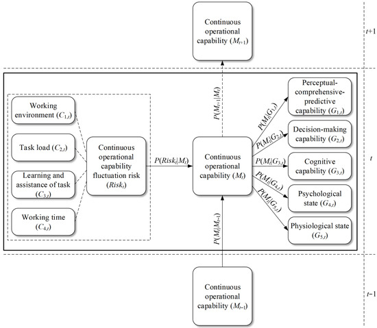
Figure 2.
Dynamic Bayesian network for the continuous operational capability evolution.
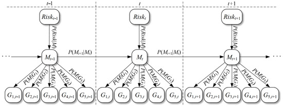
Figure 3.
BN slices in the dynamic Bayesian network.
2.2.2. Determination of Conditional Probability in the Model
As illustrated in Figure 2, in addition to the structure of the Bayesian network, it is also essential to define the conditional probabilities in the network in order to forecast the continuous operational capability evolution through the Bayesian network. While there is currently a body of research on these conditional probabilities, the majority of this research does not consider the specific operating environment of the particular team collaborative task in this study. Considering the significant characteristics of the teamwork operating environment, this paper presents a solution to the conditional probabilities in the Bayesian network using existing experimental results. The advantage of this approach is that the calculated conditional probabilities are more applicable to the team collaborative task environment under consideration in this paper. The proportion of samples that meet specific conditions among certain samples of the calculated experimental results is employed as the conditional probability in the Bayesian network. For example, the procedure for calculating the conditional probability of node Xi in state k, given that its parent node is in state j, is as follows:
where Nijk represents the number of samples that satisfy both aforementioned conditions, and Nij denotes the number of samples that meet the condition where is in state j. This paper sets the state of the Mt node to 0 and 1, indicating that there has been a decline in continuous operational capability and that there has been no decline, respectively. Similarly, the states of nodes G1,t~G5,t are defined as 0 and 1, respectively, indicating whether the result variable is more or less likely to result in a continuous operating capacity decline than the existing baseline. In other words, when the value of indicator gi,t (i = 1, 2, 3, 4, 5) is higher than the corresponding baseline value, the state of corresponding node Gi,t is 1; otherwise it is 0. This yields the conditional probabilities presented in Table 1. Similarly, the conditional probabilities related to the continuous operating capability at the previous moment can be derived as , , , and .

Table 1.
Conditional probability solution.
2.2.3. Prior Evaluation of Continuous Operational Capability Fluctuation Risk
The continuous operational capability fluctuation risk Riskt, as the parent node of the continuous operational capability Mt, overall reflects the impact of external factors on continuous operational capability. The continuous operational capability fluctuation risk Riskt can be addressed by weighting the quantitative results of each reason variable, that is,
where wj is the weight of the quantitative result cj, obtained by the author by inviting multiple scholars with relevant research experience and experimental participants to a survey, namely w1 = 0.168, w2 = 0.330, w3 = 0.247, w4 = 0.255. As Riskt represents the effect of each factor on the continuous operational capability, and is a comprehensive assessment of the continuous operational capability fluctuation risk based on the quantification of factors such as working environment, task load, and operating time, it can be concluded that the conditional probability is equal to Riskt.
2.2.4. Prediction of Continuous Operational Capability
According to the continuous operational capability evolution Bayesian network constructed above, this model analyzes the continuous operational capability evolution of team members, which is actually equivalent to solving for the probability of the state of Mt being 1. In other words, we need to determine . Firstly, utilizing the conditionally independent nature of Bayesian networks in conjunction with the full probability formula, the static Bayesian network probability distribution of Mt is derived as follows:
The static Bayesian network probability distribution is employed as a basis for the dynamic Bayesian network. Considering the time series effect, the expression for the dynamic Bayesian network probability distribution of Mt is as follows:
As a significant advantage, Bayesian networks possess the capability to effectively manage incomplete datasets, enabling the model to operate even in the absence of specific input variables. For instance, if the input variables G5,t are absent in this model, and the model identifies their absence, it will skip these variables and proceed to generate results based on the subsequent formula:
In order to verify the accuracy of the model constructed in this paper, it is also necessary to obtain the assessment of the continuous operational capability by team members themselves. To this end, a questionnaire has been devised to ascertain the subjects’ subjective evaluation of their own continuous operational capability. In light of the preceding analysis of the causes and consequences of the continuous operational capability evolution, the questionnaire requests that subjects provide a comprehensive evaluation of various dimensions, including perceptual capability, decision-making capability, cognitive capability, psychological state and physiological state. The questionnaire results can be quantified as I between 0 and 1, where 0 and 1 represent the worst and best continuous operational capability by the subjects’ own evaluations, respectively.
2.2.5. Continuous Operational Capability Prediction Method for Individual Personnel
The majority of existing continuous operational capability prediction models are universal in nature, and there is a paucity of research on models that are applicable to individual personnel. In order to address this issue, this paper seeks to develop a continuous operational capability prediction method that takes into account individual differences and is applicable to individual personnel, based on the continuous operational capability probability distribution presented above. In order to reflect individual differences, conditional probability correction factors are introduced, which serve to better reflect the characteristics of different operators. Used to compensate for the influence of individual differences, the conditional probability correction coefficients are obtained through a correlation analysis between each result variable and continuous operational capability. Hence, the accuracy of the continuous operational capability model applicable to individual personnel can be improved. The introduction of the conditional probability correction coefficients into Equation (4) results in the following expression for calculating continuous operational capability Ut:
Among them, the following applies:
In this context, the term ki,d represents the conditional probability correction factor for the result variable Gi on day d. The specific calculation method for these factors is divided into an initial stage and a subsequent stage, according to the number of days the task has been performed. In the initial stage, the limited number of test results obtained for each indicator necessitates the use of a correlation coefficient between the subjective assessment result I0 of the operator’s continuous operational capability and the quantitative result gi,0 of each result variable from previous experiments as the basis of ki,d, that is,
In the subsequent stage, because a sufficient quantity of test data has been obtained, the result can be calculated based on the correlation coefficient between the subjective evaluation of the operator’s continuous operational capability from day d − 2 to day d − 1 I(d−2)~(d−1) and the quantitative result of each result variable gi,(d−2)~(d−1), that is,
3. Experimental Design
In order to further analyze the continuous operational capability evolution of team collaborative tasks and verify the accuracy of the continuous operational capability evolution model constructed in this paper, 18 subjects, numbered as Subjects 1~18, were invited to simulate team collaborative tasks. Subjects were divided into six groups, designated A1 to A6, according to the varying duty times. Specifically, Group A1 included Subjects 1~3, Group A2 included Subjects 4~6, and so on. Each group of subjects executed the operational task on two occasions per day. The duty time for each group are illustrated in Figure 4. For instance, the duty time for group A1 is 0:00~2:00 and 12:00~14:00. Each group is responsible for completing the designated duty tasks within the specified duty hours, ensuring that there is always a group of subjects engaged in tasks at any given time of day. The total duration of the experiment is 72 h. In addition to undertaking their designated work tasks within the specified timeframes, the subjects are permitted to engage in rest or leisure activities for the remainder of the duty time.
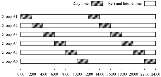
Figure 4.
Duty timeframes during the experiment.
As shown in Figure 5, in order to simulate the situation of team members’ task performance, this experimental task design is based on the common disaster relief task. Furthermore, a task system that requires teamwork has been designed, comprising four types of subtasks: perception, comprehension, prediction, and decision-making. The objective of this system is to obtain indicators of the subjects’ task abilities. The operational tasks can be classified into two categories: low-load and high-load tasks. Additionally, they can be divided into three levels based on the level of intelligent assistance: low, medium, and high. This classification allows for the simulation of the impact of complex task forms on continuous operational capability. Additionally, the working environment was subjected to continuous monitoring throughout the course of the experiment. A series of cognitive tests were conducted at regular intervals in accordance with the specifications outlined in Section 2.1.2, a range of psychological state scales were completed on a regular basis, and a series of physiological indicator tests and scale filling were carried out during the experiment.
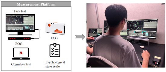
Figure 5.
Measurement Platform.
4. Results and Discussion
In order to examine the changing trend of the team member continuous operational capability and to validate the accuracy of the model constructed in this paper, a 72 h simulation experiment of team collaborative tasks was conducted. Each member was required to perform six shifts over the course of the experiment. In order to elucidate the trend of the subjects’ continuous operational capability over time, from the beginning to the end of the experiment, this paper presents the mean results of the continuous operational capability questionnaire for each group of subjects on each day, as illustrated in Table 2. Simultaneously, in order to provide a more intuitive representation of the overall changing trend of continuous operational capability, the mean results of the questionnaire for each duty for all subjects are presented in Figure 6.
Table 2.
Mean continuous operational capability per day for each group.
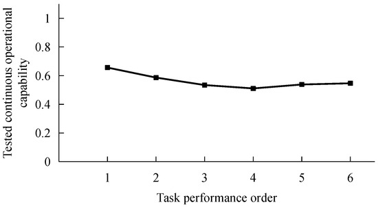
Figure 6.
Changing trend of continuous operational capability of all subjects.
As illustrated in Table 2 and Figure 6, the continuous operational capability demonstrated an overall trend of decline. From Day 1 to Day 2 and Day 3, the mean continuous operational capability of all subjects exhibited a notable decline. From one group to the next, the mean value of the continuous operational capability for each group demonstrated a decline of varying degrees from Day 1 to Day 2, with a decrease ranging from 0.06 to 0.14. From Day 1 to Day 3, with the exception of Group A2, which exhibited a minimal (less than 0.01) increase, the remaining groups exhibited a decline of varying degrees, with a decrease ranging from 0.06 to 0.13. These findings indicate a consistent decline in continuous operational capability over time, irrespective of the subject’s duty cycle.
To prove the reliability of this result, we compared it with some typical studies. The changing trend of continuous operation ability obtained in this paper is consistent with the conclusion of literature [54], which analyzed the performance of the operators when they carried out Multi-Attribute Task Battery (MATB) tasks multiple times over a period of up to 25 h. The results showed that regardless of the difficulty of the tasks, there was degradation in the task performance. This trend is consistent with the results in this paper. On the other hand, since the duration of the experiment in this paper is longer than that of the previously mentioned study, the results of this paper can be regarded as an extension of literature [54] in terms of time. Meanwhile, the results of this paper are also in line with the conclusions of the foundational literature [55]. Consequently, the changing trend of continuous operation capacity obtained in this paper is reasonable.
This paper presents a prediction model for the evolution of the team continuous operational capability applicable to individual operators. The causal relationship of the continuous operational capability evolution is comprehensively considered, and a prediction is made regarding its future evolution. In order to verify the accuracy of the model, this paper compares the results of the continuous operational capability Ut based on the model with the continuous operational capability subjective evaluation It based on the subjective evaluation scale. Due to the limitations of space, this paper presents the continuous operational capability model results and subjective evaluations of a single subject from each group, namely subjects 1, 4, 7, 11, 13 and 18, as illustrated in Figure 7.
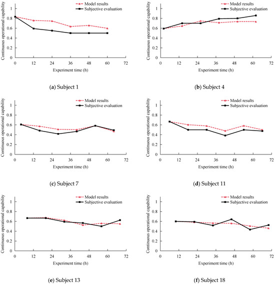
Figure 7.
Comparison of model results and subjective evaluation for a part of subjects.
It can be seen in Figure 7 that while different subjects exhibit varying degrees of proficiency in continuous operational capability, the prediction model developed in this study can provide reasonably precise estimates of their continuous operational capability at any given point in time. For each subject, the trend of the continuous operational capability by this prediction model is largely consistent with the subject’s subjective evaluation, as well as the general trend of a decrease in continuous operational capability observed across the subject population. The mean absolute error, mean relative error, and root mean square error for the aforementioned subjects are 0.062, 0.116, and 0.074, respectively. The aforementioned indicators for measuring the accuracy of the model exhibit a relatively low level, thereby substantiating the assertion that the results yielded by the continuous operational capability prediction model constructed in this paper are in alignment with the experimental results. In other words, this model can be used to predict the continuous operational capability level and its changing trend of team members.
This approach not only enhances prediction accuracy but also excels in managing situations with absent individual input data. The Bayesian network developed in this article illustrates the presumptive relationship model between continuous operational capability and associated variable, and can nevertheless yield relatively accurate answers even in the absence of a specific input variable. This article demonstrates the situation in which input variables abruptly go absent at a specific moment and presents the corresponding model output. For instance, the model can skip the data and offer the output result in accordance with Formula (5) if the input data G5,t of participant 1 is abruptly lost when the time is 36 h. This ensures that the model operates normally. Figure 8 illustrates the comparison between the output results with absent data and the original model results. The trend of changes in outcomes with missing data is fundamentally aligned with the original model results. The absolute error relative to the original model is relatively low, measuring less than 0.05, with values of 0.045, 0.037, and 0.025 from 36 h to 60 h, respectively. As time progresses and normal data input is restored, the error consistently diminishes, signifying a continual reduction in the impact of absent data.
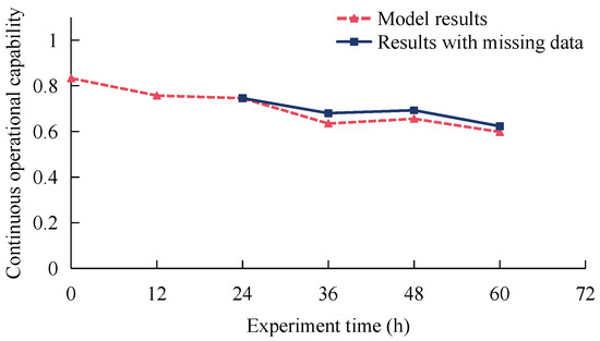
Figure 8.
Comparison between model results and results with missing data.
Additionally, the model developed in this study offers several other benefits. Firstly, the model is founded upon a discernible causal relationship of continuous operational capability and offers a comprehensive analysis of continuous operational capability from the vantage point of both cause and effect. The model considers multiple factors and is more comprehensive than existing models that rely on a single characteristic indicator. Secondly, the model fully considers individual differences and is based on the improvement on the classic Bayesian network to create a continuous operational capability evolution prediction method that is more suitable for individual operators. This ensures that the model results more accurately reflect the characteristics of the operator.
While there are notable benefits, the dynamic Bayesian network model for continuous operational capability evolution presented in this article does have certain limitations. Initially, when certain input data substantially diverges from standard levels, it might lead to considerable inaccuracies in the output results. This necessitates the fast identification of anomalous data. Secondly, a substantial correlation between variables can influence the precision of the output results. Finally, the model relies on prior knowledge, making the precise establishment of this knowledge essential for its accuracy in relation to the application of the model.
5. Conclusions
This study is concerned with the continuous operational capability evolution of team collaborative tasks. In light of the causes and consequences of continuous operational capability evolution, the Bayesian network principle is selected and refined as a means of developing a continuous operational capability prediction model tailored to the specific needs of individual operators. To validate the model, experiments were conducted to simulate the situation of team collaborative tasks. The following conclusions can be reached:
- In the context of team collaborative tasks, the subjects exhibited a general decline in continuous operational capability over time.
- The continuous operational capability prediction model developed in this study can provide a relatively accurate prediction of the continuous operational capability of team members, as well as its changing trend over time. The average absolute error, average relative error, and root mean square error are all minimal.
- This model has the advantage of handling the situation where certain input data are missing. When data is suddenly missing, the model can still output results normally with a relatively small error compared to the original model results. The impact of missing data continues to decrease as time goes on.
- This model incorporates individual differences and enhances the classic Bayesian network, establishing a methodology that is more appropriate for forecasting the continuous operational capability evolution at the level of individual operators.
Author Contributions
Conceptualization, S.W., L.P. and P.L.; methodology, S.W., L.P. and P.L.; software, S.W. and X.W.; validation, S.W., L.P., P.L. and T.J.; formal analysis, S.W.; investigation, S.W., X.W., T.J. and H.Y.; resources, S.W., L.P. and P.L.; data curation, P.L. and X.W.; writing—original draft preparation, S.W.; writing—review and editing, P.L.; visualization, S.W. and H.Y.; supervision, L.P. and P.L.; project administration, P.L. and T.J.; funding acquisition, P.L. All authors have read and agreed to the published version of the manuscript.
Funding
This research was founded by the Research Start-up Fund of the Civil Aviation University of China, grant number 3122024QD12.
Data Availability Statement
Due to the limitations of the Ethics Review Committee, these data cannot be made public to protect the privacy and confidential information of the subjects. The data presented in this study are available upon request from the corresponding author.
Acknowledgments
The authors would like to thank all subjects involved in this study.
Conflicts of Interest
The authors declare no conflicts of interest.
Appendix A
Table A1.
Quantitative and normalization of the reason indicators in Section 2.1.2.
Table A1.
Quantitative and normalization of the reason indicators in Section 2.1.2.
| Reason Indicator | Sub-Indicator | Calculation | Explanation |
|---|---|---|---|
| Working environment (c1) | Illumination (c11) | d11: color temperature (K). Based on the effect of color temperature in literature [56]. | |
| Noise (c12) | d12: sound pressure level (dB). | ||
| Gas concentration (c13) | d13: carbon dioxide concentration (ppm). d13,max, d13,min: maximum and minimum values of d13 in the experiment. | ||
| Temperature and humidity (c14) | d14: PMV by thermal comfort meter. | ||
| Task load (c2) | Current workload (c21) | d21: quantified indicator of current workload. TA: time window length (s). TR: response time for tasks at current time window (s). d21,max: maximum value of d21 in the experiment. | |
| Accumulated workload during the day (c22) | d22: quantified indicator of accumulated workload during the day. n: quantity of time window during the day. d22,max: maximum value of d22 in the experiment. | ||
| Learning and assistance of task (c3) | Task anticipation capability (c31) | d31: success rate in the pre-experiment training. | |
| Task intelligent assistance level (c32) | ob, jd, dm: intelligent assistance level for task observation, judgment, and decision-making based on OODA theory. 0, 0.5, and 1 represent low, medium and high levels, respectively. | ||
| Working time (c4) | Operating time domain (c41) | d41: relative risk rate at current time referring to literature [25]. d41,max: maximum value of d41 in the experiment. | |
| Cumulative operating time during the day (c42) | d42: relative risk rate associated with cumulated working time referring to literature [25]. d42,max: maximum value of d42 in the experiment. | ||
| Resting time since last operation (c43) | RSP: risk index based on literature [26], where tb and Tb are resting time since last operation and starting time of current operation, respectively. d43: quantified indicator of resting time since last operation. td: working time for current operation. d43,max: maximum value of d43 in the experiment. | ||
| Resting time since last operation | Cumulative resting time during the day (c44) | RSP’: risk index based on literature [26], where t’b and Tb are cumulative resting time during the day and starting time of current operation, respectively. d43: quantified indicator of cumulative resting time during the day. td: working time for current operation. d44,max: maximum value of d44 in the experiment. |
Table A2.
Quantitative and normalization of the result indicators in Section 2.1.2.
Table A2.
Quantitative and normalization of the result indicators in Section 2.1.2.
| Result Indicator | Sub-Indicator | Calculation | Explanation |
|---|---|---|---|
| Perceptual–comprehensive–predictive capability (g1) | RT of perceptual tasks (g11) | h11: RT of perceptual tasks (ms) in the experiment. h11,max: maximum value of h11 in the experiment. | |
| ACC of perceptual tasks (g12) | h12: ACC of perceptual tasks in the experiment. | ||
| RT of comprehensive tasks (g13) | h13: RT of comprehensive tasks (ms) in the experiment. h13,max: maximum value of h13 in the experiment. | ||
| ACC of comprehensive tasks (g14) | h14: ACC of comprehensive tasks in the experiment. | ||
| RT of predictive tasks (g15) | h15: RT of predictive tasks (ms) in the experiment. h15,max: maximum value of h15 in the experiment. | ||
| ACC of predictive tasks (g16) | h16: ACC of predictive tasks in the experiment. | ||
| Decision-making capability (g2) | RT of decision-making tasks (g21) | h21: RT of decision-making tasks (ms) in the experiment. h21,max: maximum value of h21 in the experiment. | |
| ACC of decision-making tasks (g22) | h22: ACC of decision-making tasks in the experiment. | ||
| Cognitive capability (g3) | RT of PVT tests (g31) | h31: RT of PVT tests (ms) in the experiment. h31,max: maximum value of h31 in the experiment. | |
| ACC of PVT tests (g32) | h32: ACC of PVT tests in the experiment. | ||
| RT of Stroop tests (g33) | h33: RT of Stroop tests (ms) in the experiment. h33,max: maximum value of h33 in the experiment. | ||
| ACC of Stroop tests (g34) | h34: ACC of Stroop tests in the experiment. | ||
| RT of GO-NOGO tests (g35) | h35: RT of GO-NOGO tests (ms) in the experiment. h35,max: maximum value of h35 in the experiment. | ||
| ACC of GO-NOGO tests (g36) | h36: ACC of GO-NOGO tests in the experiment. | ||
| RT of implicit-emotion tests (g37) | h37: RT of implicit-emotion tests (ms) in the experiment. h37,max: maximum value of h37 in the experiment. | ||
| ACC of implicit-emotion tests (g38) | h38: ACC of implicit-emotion tests in the experiment. | ||
| Psychological state (g4) | Alertness (g41) | h41: KSS score. | |
| Task satisfaction (g42) | h42: job satisfaction scale score. | ||
| Physiological state (g5) | Changing rate of pupil diameter (g51) | h51: pupil diameter in the experiment. h51,bl: baseline data of pupil diameter before the experiment. | |
| Changing rate of fixation duration (g52) | h52: fixation duration in the experiment. h52,bl: baseline data of fixation duration before the experiment. | ||
| Changing rate of heart rate (g53) | h53: heart rate in the experiment. h53,bl: baseline data of heart rate before the experiment. | ||
| Changing rate of underarm temperature (g54) | h54: underarm temperature in the experiment. h54,bl: baseline data of underarm temperature before the experiment. | ||
| Sleep quality score (g55) | h55: sleep quality score by the wristband. | ||
| Resting time since last operation | Physical comfort scale (g56) | h56: physical comfort scale score. |
References
- Hu, X.; Lodewijks, G. Detecting fatigue in car drivers and aircraft pilots by using non-invasive measures: The value of differentiation of sleepiness and mental fatigue. J. Saf. Res. 2020, 72, 173–187. [Google Scholar] [CrossRef] [PubMed]
- Wu, E.Q.; Deng, P.Y.; Qiu, X.Y.; Tang, Z.R.; Zhang, W.M.; Zhu, L.M.; Ren, H.; Zhou, G.R.; Sheng, R.S.F. Detecting Fatigue Status of Pilots Based on Deep Learning Network Using EEG Signals. IEEE Trans. Cogn. Dev. Syst. 2021, 13, 575–585. [Google Scholar] [CrossRef]
- Tian, L.J.; Chen, T.T.; Wang, J.B. Internal control, safety culture and aviation safety. China Saf. Sci. J. 2016, 26, 1–6. [Google Scholar] [CrossRef]
- Azam, K.; Shakoor, A.; Shah, R.A.; Khan, A.H.; Shah, S.A.A.; Khalil, M. Comparison of fatigue related road traffic crashes on the national highways and motorways in Pakistan. J. Eng. Appl. Sci. 2014, 33, 47–54. [Google Scholar]
- Savas, B.K.; Becerikli, Y. Real Time Driver Fatigue Detection System Based on Multi-Task ConNN. IEEE Access 2020, 8, 12491–12498. [Google Scholar] [CrossRef]
- Weelden, E.; Alimardani, M.; Wiltshire, T.J.; Louwerse, M.M. Aviation and neurophysiology: A systematic review. Appl. Ergon. 2022, 105, 103838. [Google Scholar] [CrossRef]
- Freitas, A.; Almeida, R.; Gonçalves, H.; Conceição, G.; Freitas, A. Monitoring fatigue and drowsiness in motor vehicle occupants using electrocardiogram and heart rate—A systematic review. Transp. Res. Part F Psychol. Behav. 2024, 103, 586–607. [Google Scholar] [CrossRef]
- Darzi, A.; Gaweesh, S.M.; Ahmed, M.M.; Novak, D. Identifying the Causes of Drivers’ Hazardous States Using Driver Characteristics, Vehicle Kinematics, and Physiological Measurements. Front. Neurosci. 2018, 12, 568. [Google Scholar] [CrossRef]
- Mansikka, H.; Virtanen, K.; Harris, D.; Simola, P. Fighter pilots’ heart rate, heart rate variation and performance during an instrument flight rules proficiency test. Appl. Ergon. 2016, 56, 213–219. [Google Scholar] [CrossRef]
- Lu, K.; Karlsson, J.; Dahlman, A.S.; Sjoqvist, B.A.; Candefjord, S. Detecting Driver Sleepiness Using Consumer Wearable Devices in Manual and Partial Automated Real-Road Driving. IEEE Trans. Intell. Transp. Syst. 2022, 23, 4801–4810. [Google Scholar] [CrossRef]
- Lopez, M.B.; del-Blanco, C.R.; Garcia, N. Detecting Exercise-Induced Fatigue Using Thermal Imaging and Deep Learning. In Proceedings of the International Conference on Image Processing, Montreal, QC, Canada, 28 November–1 December 2017. [Google Scholar] [CrossRef]
- Quddus, A.; Zandi, A.S.; Prest, L.; Comeau, F.J.E. Using long short term memory and convolutional neural networks for driver drowsiness detection. Accid. Anal. Prev. 2021, 156, 106107. [Google Scholar] [CrossRef]
- He, J.; William, C.; Yang, Y.; Lu, J.S.; Wu, X.H.; Peng, K.P. Detection of driver drowsiness using wearable devices: A feasibility study of the proximity sensor. Appl. Ergon. 2017, 65, 473–480. [Google Scholar] [CrossRef]
- Lees, T.; Chalmers, T.; Burton, D.; Zilberg, E.; Penzel, T.; Lal, S.; Lal, S. Electrophysiological Brain-Cardiac Coupling in Train Drivers during Monotonous Driving. Int. J. Environ. Res. Public Health 2021, 18, 3741. [Google Scholar] [CrossRef]
- Markus, G.; David, S.; Thomas, W.; Natividad, M.M.; Ralf, S. ECG sensor for detection of driver’s drowsiness. Procedia Comput. Sci. 2019, 159, 1938–1946. [Google Scholar] [CrossRef]
- Wu, X.Y.; Cang, N.M.; Yu, W.J.; Wang, Z.C.; Zhao, H.L.; Liu, J.L. Driver’s EEG Eye Movement Fatigue Detection Based on CMAC. In Proceedings of the International Conference on Intelligent Informatics and Biomedical Sciences (ICIIBMS), Shanghai, China, 21–24 November 2019. [Google Scholar] [CrossRef]
- Shafer, G.; Shenoy, P. Probability propagation. Ann. Math. Artif. Intell. 1990, 2, 327–352. [Google Scholar] [CrossRef]
- Pearl, J. Probabilistic Reasoning in Intelligent Systems: Networks of Plausible Inference; Morgan Kaufmann: San Mateo, CA, USA, 1998. [Google Scholar]
- Zhang, J.; Cao, X.D.; Wang, X.; Pang, L.P.; Liang, J.; Zhang, L. Physiological Responses to Elevated Carbon Dioxide Concentration and Mental Workload during Performing MATB Tasks. Build. Environ. 2021, 195, 107752. [Google Scholar] [CrossRef]
- Ivosevic, J.; Bucak, T.; Andrasi, P. Effects of Interior Aircraft Noise on Pilot Performance. Appl. Acoust. 2018, 139, 8–13. [Google Scholar] [CrossRef]
- Zhang, J.; Pang, L.P.; Cao, X.D.; Wanyan, X.R.; Wang, X.; Liang, J.; Zhang, L. The Effects of Elevated Carbon Dioxide Concentration and Mental Workload on Task Performance in an Enclosed Environmental Chamber. Build. Environ. 2020, 178, 106938. [Google Scholar] [CrossRef]
- Alahmer, A.; Omar, M.; Mayyas, A.R.; Qattawi, A. Analysis of vehicular cabins’ thermal sensation and comfort state, under relative humidity and temperature control, using Berkeley and Fanger models. Build. Environ. 2012, 48, 146–163. [Google Scholar] [CrossRef]
- Maik, F.; Lee, S.Y.; Paul, B.; Wayne, M.; Faulhaber, A.K. The Influence of Training Level on Manual Flight in Connection to Performance, Scan Pattern, and Task Load. Cogn. Technol. Work 2021, 23, 715–730. [Google Scholar] [CrossRef]
- Trippas, J.R.; Spina, D.; Scholer, F.; Awadallah, A.H.; Bailey, P.; Bennett, P.N.; White, R.W.; Liono, J.; Ren, Y.; Salim, F.D.; et al. Learning about Work Tasks to Inform Intelligent Assistant Design. In Proceedings of the Conference on Human Information Interaction and Retrieval, Scotland, UK, 10–14 March 2019. [Google Scholar] [CrossRef]
- Spencer, M.B.; Robertson, K.A.; Folkard, S. The Development of a Fatigue/Risk Index for Shiftworkers; The Health and Safety Executive; HSE Books: London, UK, 2006.
- Rogers, A.S.; Spencer, M.B.; Stone, B.M. Validation and Development of a Method for Assessing the Risks Arising from Mental Fatigue; The Health and Safety Executive; HSE Books: London, UK, 1999.
- Hegarty, M. Ability and Sex Differences in Spatial Thinking: What Does the Mental Rotation Test Really Measure? Psychon. Bull. Rev. 2018, 25, 1212–1219. [Google Scholar] [CrossRef]
- Wai, J.; Lubinski, D.; Benbow, C.P. Spatial Ability for STEM Domains: Aligning over 50 Years of Cumulative Psychological Knowledge Solidifies Its Importance. J. Educ. Psychol. 2009, 101, 817–835. [Google Scholar] [CrossRef]
- Schmidt, F.L.; Hunter, J.E. General mental ability in the world of work: Occupational attainment and job performance. J. Personal. Soc. Psychol. 2004, 86, 162–173. [Google Scholar] [CrossRef]
- Dalal, D.K.; Diab, D.L.; Zhu, X.; Hwang, T. Understanding the Construct of Maximizing Tendency: A Theoretical and Empirical Evaluation. J. Behav. Decis. Mak. 2015, 28, 437–450. [Google Scholar] [CrossRef]
- Biondi, F.N.; Cacanindin, A.; Douglas, C.; Cort, J. Overloaded and at Work: Investigating the Effect of Cognitive Workload on Assembly Task Performance. Hum. Factors 2021, 63, 813–820. [Google Scholar] [CrossRef] [PubMed]
- Biondi, F.N.; Balasingam, B.; Ayare, P. On the Cost of Detection Response Task Performance on Cognitive Load. Hum. Factors 2021, 63, 804–812. [Google Scholar] [CrossRef]
- Madrid, H.P.; Diaz, M.T.; Leka, S.; Leiva, P.I.; Barros, E. A Finer Grained Approach to Psychological Capital and Work Performance. J. Bus. Psychol. 2018, 33, 461–477. [Google Scholar] [CrossRef]
- Schmidt, C.; Collette, F.; Cajochen, C.; Peigneux, P. A Time to Think: Circadian Rhythms in Human Cognition. Cogn. Neuropsychol. 2007, 24, 755–789. [Google Scholar] [CrossRef]
- Cao, X.D.; Li, P.; Zhang, J.; Pang, L.P. Associations of human cognitive abilities with elevated carbon dioxide concentrations in an enclosed chamber. Atmosphere 2022, 13, 891. [Google Scholar] [CrossRef]
- Zhang, X.; Wargocki, P.; Lian, Z.; Thyregod, C. Effects of Exposure to Carbon Dioxide and Bioeffluents on Perceived Air Quality, Self-Assessed Acute Health Symptoms, snd Cognitive Performance. Indoor Air 2017, 27, 47–64. [Google Scholar] [CrossRef]
- Zhang, X.; Wargocki, P.; Lian, Z. Physiological Responses during Exposure to Carbon Dioxide and Bioeffluents at Levels Typically Occurring Indoors. Indoor Air 2017, 27, 65–77. [Google Scholar] [CrossRef] [PubMed]
- Spengler, J.D.; Vallarino, J.; Mcneely, E.; Estephan, H. In-Flight/Onboard Monitoring: ACER’s Component for ASHRAE (2012); Harvard School of Public Health: Boston, MA, USA, 2020. [Google Scholar]
- Zhang, S.; Lin, Z. Extending Predicted Mean Vote using adaptive approach. Build. Environ. 2020, 171, 106665. [Google Scholar] [CrossRef]
- Chen, T.P. Computer Vision Workload Analysis: Case Study of Video Surveillance Systems. Intel Technol. J. 2005, 9, 109. [Google Scholar] [CrossRef]
- Schechtman, G.M. Manipulating the OODA Loop: The Overlooked Role of Information Resource Management in Information Warfare; Barakaldo Books: Barakaldo, Spain, 2012. [Google Scholar]
- Johnson, J. Automating the OODA Loop in the Age of Intelligent Machines: Reaffirming the Role of Humans in Command-and-control Decision-Making in the Digital Age. Def. Stud. 2022, 23, 43–67. [Google Scholar] [CrossRef]
- Jones, M.J.; Dunican, I.C.; Murray, K.; Peeling, P.; Dawson, B.; Halson, S.; Miller, J.; Eastwood, P.R. The Psychomotor Vigilance Test: A Comparison of Different Test Durations in Elite Athletes. J. Sports Sci. 2018, 36, 2033–2037. [Google Scholar] [CrossRef]
- Basner, M.; Dinges, D.F. An adaptive-duration version of the PVT accurately tracks changes in psychomotor vigilance induced by sleep restriction. Sleep 2012, 35, 193–202. [Google Scholar] [CrossRef][Green Version]
- Bajaj, J.S.; Heuman, D.M.; Sterling, R.K.; Sanyal, A.J.; Siddiqui, M.; Matherly, S.; Luketic, V.; Stravitz, R.; Fuchs, M.; Thacker, L.R.; et al. Validation of Encephal App, smartphone-based Stroop test, for the diagnosis of covert hepatic encephalopathy. Clin. Gastroenterol. Hepatol. 2015, 13, 1828–1835. [Google Scholar] [CrossRef]
- Erdodi, L.A.; Sagar, S.; Seke, K.; Zuccato, B.G.; Schwartz, E.S.; Roth, R.M. The Stroop Test as a Measure of Performance Validity in Adults Clinically Referred for Neuropsychological Assessment. Psychol. Assess. 2018, 30, 755–766. [Google Scholar] [CrossRef]
- Criaud, M.; Boulinguez, P. Have we been asking the right questions when assessing response inhibition in go/no-go tasks with fMRI? A meta-analysis and critical review. Neurosci. Biobehav. Rev. 2013, 37, 11–23. [Google Scholar] [CrossRef]
- Tania, M.; Giulia, B. Response Inhibition in Problematic Social Network Sites Use: An ERP Study. Cogn. Affect. Behav. Neurosci. 2021, 21, 868–880. [Google Scholar] [CrossRef]
- Bartoszek, G.; Cervone, D. Toward an implicit measure of emotions: Ratings of abstract images reveal distinct emotional states. Cogn. Emot. 2016, 31, 1377–1391. [Google Scholar] [CrossRef] [PubMed]
- Roefs, A.; Huijding, J.; Smulders, F.T.Y.; MacLeud, C.M.; de Jong, P.J.; Wires, R.W.; Jansen, A.T.M. Implicit measures of association in psychopathology research. Psychol. Bull. 2011, 137, 149–193. [Google Scholar] [CrossRef]
- Gyurak, A.; Gross, J.J.; Etkin, A. Explicit and implicit emotion regulation: A dual-process framework. Cogn. Emot. 2011, 25, 400–412. [Google Scholar] [CrossRef]
- Loew, M.; Niel, K.; Burlison, J.D.; Russell, K.M.; Karol, S.E.; Talleur, A.C.; Christy, L.A.N.N.; Johnson, L.M.; Crabtree, V.M. A quality improvement project to improve pediatric medical provider sleep and communication during night shifts. Int. J. Qual. Health Care 2018, 31, 633–638. [Google Scholar] [CrossRef]
- Mulhall, M.D.; Sletten, T.L.; Magee, M.; Stone, J.E.; Ganesan, S.; Collins, A.; Anderson, C.; Lockley, S.W.; Howard, M.E.; Rajaratnam, S.M.W. Sleepiness and driving events in shift workers: The impact of circadian and homeostatic factors. Sleep 2019, 42, zsz074. [Google Scholar] [CrossRef] [PubMed]
- Kong, Y.; Posada-Quintero, H.F.; Gever, D.; Bonacci, L.; Chon, K.H.; Bolkhovsky, J. Multi-Attribute Task Battery Configuration to Effectively Assess Pilot Performance Deterioration During Prolonged Wakefulness. Inform. Med. Unlocked 2022, 28, 100822. [Google Scholar] [CrossRef]
- Virtanen, M.; Singh-Manoux, A.; Ferrie, J.E.; Gimeno, D.; Marmot, M.G.; Elovainio, M.; Jokela, M.; Vahtera, J.; Kivimäki, M. Long Working Hours and Cognitive Function: The Whitehall II Study. Am. J. Epidemiol. 2009, 169, 596–605. [Google Scholar] [CrossRef]
- Weng, Z.X.; Wei, L.Z.; Song, J.; Wang, X.; Liang, J.; Zhang, L. Effect of Enclosed Lighting Environment on Work Performance and Visual Perception. In Proceedings of the 2020 17th China International Forum on Solid State Lighting & 2020 International Forum on Wide Bandgap Semiconductors China (SSLChina: IFWS), Shenzhen, China, 23–25 November 2020. [Google Scholar] [CrossRef]
Disclaimer/Publisher’s Note: The statements, opinions and data contained in all publications are solely those of the individual author(s) and contributor(s) and not of MDPI and/or the editor(s). MDPI and/or the editor(s) disclaim responsibility for any injury to people or property resulting from any ideas, methods, instructions or products referred to in the content. |
© 2025 by the authors. Licensee MDPI, Basel, Switzerland. This article is an open access article distributed under the terms and conditions of the Creative Commons Attribution (CC BY) license (https://creativecommons.org/licenses/by/4.0/).