Abstract
This paper proposes a numerical technique to study dynamical systems and uncover new behaviors in chaotic fractional-order models, a field that continues to attract significant research interest due to its broad applicability and the ongoing development of innovative methods. Through various types of simulations, this approach is able to uncover novel dynamic behaviors that were previously undiscovered. The results guarantee that initial conditions and fractional-order derivatives have a significant contribution to system dynamics, thus distinguishing fractional systems from traditional integer-order models. The approach demonstrated has excellent consistency with traditional approaches for integer-order systems while offering higher accuracy for fractional orders. Consequently, this approach serves as a powerful and efficient tool for studying complex chaotic models. Fractional-order dynamical systems (FDSs) are particularly noteworthy for their ability to model memory and hereditary characteristics. The method identifies new complex phenomena, including new chaos, unusual attractors, and complex time-series patterns, not documented in the existing literature. We use Lyapunov exponents, bifurcation analysis, and Poincaré sections to thoroughly investigate the system dynamics, with particular emphasis on the effect of fractional-order and initial conditions. Compared to traditional integer-order approaches, our approach is more accurate and gives a more efficient device for facilitating research on fractional-order chaos.
Keywords:
fractional-order systems; chaos; dynamical analysis; Rössler attractors; numerical methods MSC:
26A33; 34C28; 65P10; 74H65; 65P20
1. Introduction
By extending differentiation and integration to noninteger orders, fractional calculus makes it possible for models to account for effects that are dependent on memory and history. Caputo-type fractional derivatives enhance disease dynamics modeling and stability analysis (Saadeh et al. [1]). Abdoon and Alzahrani [2] demonstrated how fractional operators improve epidemiological modeling, while Hilfer [3] emphasized physics applications like diffusion and viscoelasticity. Gündoğdu and Joshi [4] and Ferrari et al. [5] used fractional calculus to study cancer dynamics and separation processes, demonstrating how well it captures intricate, real-world behavior. All things considered, fractional derivatives are more accurate and flexible than traditional integer-order models, which makes them ideal for engineering, biological, and chaotic systems.
This growth is sure to be a result of the special features of fractional calculus, including its ability to effectively describe complex systems with memory influence and non-local interactions, qualities that are well beyond the ability of conventional integer-order models to mimic [6,7,8].
An increasing number of critical research studies in this field confirm its wide range of applications and underscore its growing important in both theoretical and practical contexts [9,10,11,12].
Over time, researchers began exploring fractional calculus because certain systems showed behaviors that traditional models struggled to represent accurately. Their studies have shown that fractional calculus is useful for understanding complex chaotic systems, designing electric circuits with changing properties, and developing secure encryption methods. These findings show that fractional calculus is important for improving response systems, understanding complex spinning behaviors, and accurately explaining detailed patterns in many areas such as science, engineering, biology, chemistry, and related mathematics fields [13,14,15,16].
The Caputo derivative stands out among all fractional derivatives because it can naturally account for memory and heredity effects, which are essential for accurate depictions of complex systems [17,18]. Compared to other definitions, the Caputo derivative is numerically more efficient, produces higher accuracy and smoother solutions, and has improved convergence [19,20,21]. In many areas, including science and epidemiology, the Caputo derivative has proven useful for modeling dynamic systems, offering deeper insights than traditional methods [22,23,24,25].
The Rössler system, developed in the 1970s, is a simple model of chaos theory made up of three nonlinear differential equations [26]. Inverting the modified Rössler system symmetrically changes the way the system behaves, especially with respect to its stability. This modification supports the development of control strategies, stability analysis, and the study of chaos. Researchers have been increasingly focused on this variation, primarily because symmetry provides a unique perspective for studying how the system evolves. The equations for this inverted case are shown as follows:
In this system, the state variables , and Z evolve dynamically, while the parameters , , and determine the control dynamical system. One of the enormous advantages of using Caputo fractional derivatives “” is that they can capture memory effects. This advantage is due to the fractional order, which gives adaptive parameters that can be highly adjusted to capture the history-dependent nature of the system. Moreover, the Caputo derivatives keep the solutions smooth, and this renders them very convenient in the study of chaotic dynamics. These are the characteristics that allow dynamic behaviors to be better defined and in greater detail. Therefore, it is best to use the Caputo fractional derivatives to model complex systems where integer-order derivatives are insufficient:
The parameters are set as , and , with initial conditions given by (see [27]).
As defined in Equation (2), the fractional Rössler system extends the classical chaotic model by introducing memory effects, which are captured using Caputo fractional derivatives.
According to the memory effects, the whole history of the system, not just its current state, determines its state at any particular instant. It has been increasingly recognized that fractional-order models can account for memory effects, which is not something standard models do particularly well. This capability turns out to be useful when dealing with things like anomalous diffusion or long-term correlations—patterns often seen in physical or biological systems. Also, being able to adjust the fractional order affords researchers some control over how the system behaves under external changes. That kind of tuning might even lead to dynamics that would not normally show up in traditional models.
Fractional-order chaotic systems have garnered a lot of interest due to their enhanced ability to model the memory and hereditary aspects seen in nature. Of all the models, the fractional-order Rössler model has emerged as a fundamental one for analyzing sophisticated dynamic phenomena and various characteristics of the system, such as chaos and hyperchaos [28,29,30,31,32,33].
Over the last few years, researchers have become increasingly interested in fractional-order dynamical systems (FDSs) due to their utility in modeling memory and hereditary effects, features that often occur in complex physical or biological systems. Much of the recent work has looked into behaviors like chaos, strange attractors, and time-series responses, using tools such as Lyapunov exponents and bifurcation diagrams to better understand system dynamics. Numerical simulations have also played an important role, especially when analytical solutions are impractical. One area that still seems underexplored is the use of the Poincaré section (PS) in FDS, even though it could help simplify how we interpret the motion of these systems in phase space.
Table 1 and Figure 1 provides a summary of previous studies on fractional-order dynamical systems, many of which focused on basic aspects such as system definitions and limited discussions of chaotic (CH), nonchaotic (NCH), and bifurcation (BF) behaviors [27,34,35,36,37,38]. More detailed analyses, such as symmetry analysis (SA) and time series (TS) evaluation, began to appear in later work, notably in [39]. This study incorporated several dynamic aspects, including symmetry analysis (SA) and time series (TS) examination. However, only the current study demonstrates a complete integration of all the features considered, including Lyapunov exponents (LE), bifurcation (BF), and numerical simulations (NS), highlighting its distinct contribution. Our work has been compared with all these references, and its distinction became evident in terms of the completeness of the analysis and the diversity of the dynamic characteristics studied.

Table 1.
Comparison of studies on fractional-order Rössler systems and chaos.
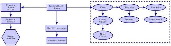
Figure 1.
Graphical abstract of perturbed dynamical system analysis.
This work highlights the crucial role of fractional derivatives and initial conditions by introducing a numerical method that uncovers previously unobserved behaviors in chaotic fractional-order systems. The technique provides an effective tool for furthering research in fractional-order chaos by more accurately revealing complex dynamics and novel attractors than traditional integer-order models.
There are many numerical methods that have been proposed for solving fractional-order differential equations, but two that are well-known include the Grünwald–Letnikov algorithm of Petras [40] and Diethelm’s algorithm [41], which Tavazoei [42] later studied and improved. These approaches have proven key to improving the computational handling of fractional systems by providing consistent ways to approximate fractional derivatives.
2. Preliminaries
In this section, we present the fundamental definitions of the fractional operator employed in this study, where The gamma function is denoted by
Definition 1
([43]). The Riemann–Liouville fractional integral of order α for a given function ℓ is defined by
Definition 2
([43]). The Riemann–Liouville fractional derivative of order α for a given function ℓ is expressed as
Definition 3
([43]). The Caputo fractional derivative of order α for a given function ℓ is formulated by
3. Dynamical System
In the past few years, more researchers have begun exploring fractional-order dynamical systems. This growing interest seems to stem from the fact that these systems can, in many cases, reflect the behavior of complicated real-world processes more precisely than the standard models that rely on integer-order dynamics. Such systems are particularly effective in capturing hereditary and memory-dependent properties that are common in physical and biological scenarios. This section is dedicated to the investigation of a dynamical system described by fractional derivatives in the Caputo sense in Equation (1).
Theorem 1.
Every solution of the system (1) with positive initial conditions , , exists and is unique in the interval .
Let , and define the vector function such that
The system (6) can now be written in the autonomous form
where:
- maps the positive real line to 3D space.
- for (i.e., each component is infinitely differentiable).
- Continuity: Q is fully continuous because each is composed of elementary functions.
- Lipschitz Condition: Q is locally Lipschitz in the positive quadrant
This follows from the smoothness Q and boundedness of derivatives in W. By the Picard–Lindelöf theorem, the system with initial conditions has a unique solution extending to .
4. Fractional-Order Dynamical Analysis
To gain deeper insight into the system’s dynamics, we investigate the rich dynamical behavior of system (2) under a range of initial conditions, parameter values, and fractional orders. Particular emphasis is placed on identifying novel chaotic attractors that highlight the system’s inherent sensitivity and complex dynamics.
The corresponding Jacobian matrix of system (2) is given by
Equilibrium:
Jacobian at :
Characteristic polynomial at :
Eigenvalues at :
Stability: The equilibrium is unstable. indicates stability along one direction, while show weakly unstable oscillations.
Equilibrium:
Jacobian at :
Characteristic polynomial at :
Eigenvalues at :
Stability: Since there is one positive real eigenvalue (), the equilibrium is unstable (a saddle-focus).
To analyze the local stability of the fractional-order system, we define
where J is the Jacobian matrix evaluated at the equilibrium point, and are the corresponding fractional orders.
The equilibrium point is asymptotically stable if all eigenvalues satisfy
If inequality holds, the system is asymptotically stable. Otherwise, chaos:
As a consequence, it can be concluded that the solution of this linear system is asymptotically stable if all the roots of the equation satisfy the condition
We compute
Equilibrium Point
Equilibrium Point
Interpretation : stable for ; : unstable (positive real eigenvalue)
In Table 2, the fractional-order system shows varied dynamics as changes. For , is stable, while is unstable. Near (e.g., ), exhibits bounded chaos and loses stability, highlighting the system’s sensitivity to fractional order and the emergence of complex dynamics.
Table 2.
The resultant dynamics of the fractional-order system around the relevant equilibria.
4.1. Application of Numerical CFD to the Rössler System
This section explores the use of straightforward numerical methods to estimate solutions to Caputo fractional-order systems. The system can be expressed as
where, . Let approximate at .
Using the numerical method in [41,42], Equation (21), this method studies the existence, uniqueness, and stability of fractional-order equations with physically meaningful Caputo conditions and highlights the complex behaviors of fractional-order dynamical systems, with a focus on chaos. It can be reformulated as follows:
where , and Equation (22) then
where , and Equation (22) then
From Equations (23) and (24)
Lagrange polynomial interpolation is applied to obtain an approximate solution to Equation (21) as
The solutions of the 3D constant-order fractional system involving the Caputo derivative can be expressed as follows:
and .
and .
and .
These findings support the notion that the numerical solution accurately represents the system’s behavior, and sensitivity to initial conditions and order fractionality are observable, specifically in sign reversal and symmetry between solutions for the two cases. In addition, the discrepancies between the results of integer-order and fractional-order depict the memory effect of fractional systems. Here, we present the system dynamics (2) in various initial conditions and fractional orders according to the numerical solutions in Table 3 and Table 4. Table 3 is for with in , and Table 4 is for with in . In both cases, the numerical solutions consistently converge as the step size h decreases, echoing the stability and accuracy of the numerical scheme used. From one-step refinement to the next, the solution changes insignificantly, showing very good numerical stability. The Adams–Bashforth method (ABM) also gives similar results but with a relatively larger deviation, particularly in component Y, which may be due to limitations in capturing long-term or memory-dependent effects, particularly for the fractional-order case.
Table 3.
Numerical solutions of system (2) for where , and .
Table 4.
Numerical solutions of system (2) for where , and .
The proposed numerical algorithm extends existing methods by introducing a fractional derivative treatment. Comparative experiments with classical methods of Adams–Bashforth–Moulton (ABM) demonstrate its effectiveness, with detailed results.The numerical results extend the dynamic behaviors. These are supported by stability and bifurcation analyses. The solution reflects system behavior sensitivity to the initial conditions and fractional order, especially in sign changes and symmetry between cases. The solutions consistently converge as the step size h decreases, showing good numerical stability.
4.2. Bifurcation
The dynamical behavior of the Rössler system (2) is strongly dependent on the value of the fractional order , and we conduct extensive numerical simulations employing the fractional order as a control parameter, providing a comprehensive understanding of the system’s dynamics. The system may illustrate various dynamic behaviors for the same parameter values used above, namely . The figures were drawn with the help of the package of MATLAB software (R2024a).
Two complementary approaches are mainly used to analyze the system’s qualitative behavior after eliminating transient dynamics arising from the initial conditions . In order to show dynamic transitions of the system, the one-parameter bifurcation diagram is first created by varying the fractional order as a single control parameter and then depicting maxima (green) and minima (pink) with respect to over the range (Figure 2a). Second, by selecting different values of the fractional order , phase-space diagrams are produced in Figure 2b–e to emulate the regime of the system at each value of .
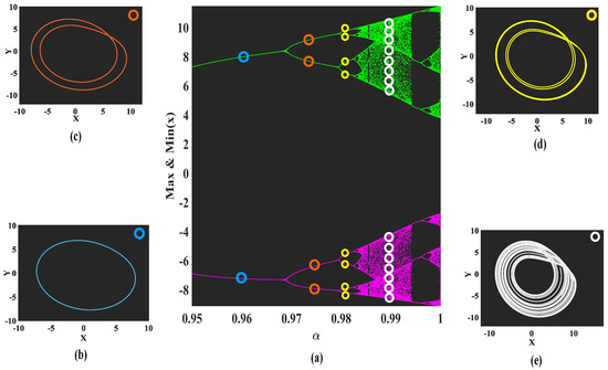
Figure 2.
Panel (a) shows the bifurcation diagram of system (2) under the increasing variation of the fractional order , while panels (b–e) present the phase spaces corresponding to the cyan, orange, yellow, and white circles, respectively.
In Figure 2a, the bifurcation diagram shows clear transitions from stable attractors (periodic solutions) at lower values of to chaotic attractors (chaotic dynamics) at higher values of , demonstrating the destabilizing effect of increasing the fractional order. Accordingly, four values of are chosen to represent the prevalent regimes over the selected range of the fractional order.
For lower fractional-order , the system oscillates on an attractor. This attractor is cyclic (periodic), whereby the dynamic behavior takes the form of a period-1 cycle as the phase space shown in Figure 2b. When the fractional order is increasingly varied, the system moves from the period-1 attractor to a period-2 attractor as plotted in Figure 2c at . The transition from the period-1 cycle to the period-2 cycle occurs because of the existence of period-doubling. This leads the system to move from a regime of period-1 to a regime of period-2.
An additional increase in fractional order leads to another occurrence of period-doubling as observed in Figure 2d when , which depicts that the system oscillates on an attractor forming as a period-4 cycle. This proves that increases in the value of fractional order can affect the dynamic behavior of the system (2) and increase its complexity, whereby the system dynamically becomes a regime of period-4.
For higher fractional-order , the bifurcation diagram’s dense clustering of maxima and minima points indicates the system’s chaotic nature. The system’s chaotic nature is further supported by the phase space shown in Figure 2e, which displays a dense chaotic attractor. This indicates a strong sensitivity of the system to initial conditions, leading to unexpected long-term behavior. Plus, it experiences a cascade of period-doublings as the fractional order rises, gradually transitioning towards less organized behavior as the cyclic attractor of period-4 enters a chaotic regime.
To sum up this section, the fractional-order functions as a control parameter that affects the system’s qualitative behavior and dictates its regimes. Therefore, it is demonstrated that lower fractional orders help in the regulation of fluctuations, resulting in dynamics that are regular and stable. The system (2) eventually loses stability as the fractional orders grow because it depends more on its present state than on effects from the past. Overall, we synthesize these findings to show that greater fractional orders cause instability and chaos in the Rössler system (2), while lower fractional orders encourage stability.
4.3. Poincaré Sections
There is no doubt that the study of the Poincaré section serves as a crucial tool for researchers to understand and identify complex dynamics. Here, the Poincaré section is studied in order to simplify the presented phase spaces by capturing only the locations at which the dynamic intersects a chosen surface. This makes irregular dynamics especially easier to see and understand the increasing complexity of dynamics as the increasing variation of the fractional-order in the Rössler system (2).
The Poincaré section provides a brief glimpse of the underlying structure of cyclic attractors and chaotic attractors that could otherwise be hidden in the complete phase-space diagrams by merely tracking the crossing points. Therefore, we here depict the regular and complex dynamics as Poincaré fixed points (red dots) on Poincaré sections (black sections) as drawn in Figure 3a–d.
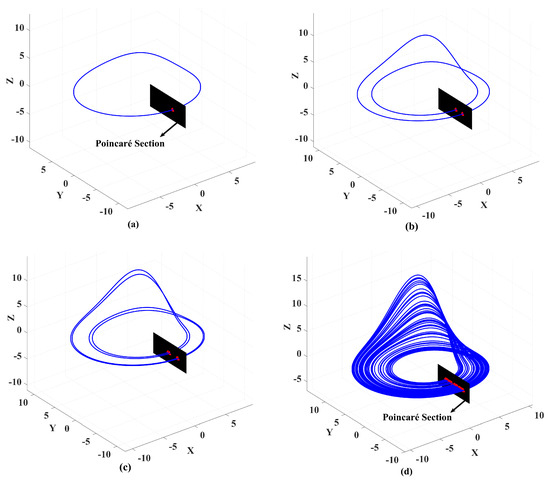
Figure 3.
(a–d) The 3D phase spaces corresponding to the phase spaces in Figure 2b–e with the relevant Poincaré sections in black at the same use fractional-order values.
It has already been demonstrated in Section 4.2 that the system settles into a variety of different-period cyclic attractors as well as chaos depending on the value of . The 3D phase spaces below depicted in Figure 3a–d reflect the locations of Poincaré fixed points in the Poincaré sections, corresponding to the dynamic behaviors already presented in Figure 2b–e for the same values of the fractional-orders and initial conditions.
In Figure 3a, fixing the fractional-order at tells that there exists a period-1 cycle that manifests itself as a single red dot representing a Poincaré fixed point in the Poincaré section. The reason for this is because the period-1 cycle always intersects the Poincaré section at the same location, as it returns to the same state in the 3D phase space after precisely one complete cycle.
If the fractional-order is further raised (), the Poincaré section shows two different red dots that correspond to two Poincaré fixed points as seen in Figure 3b. This occurs because instead of returning to the same location at the end of each cycle (as occurred in the period-1 cycle), the dynamic alternates between two dots after intersecting the black section twice in a repeating pattern. The cycle thus alternates between these two red dots, resulting in a “period-2 cycle” in the Poincaré section.
Figure 3c reveals that there are four different red dots in the Poincaré section that represent a period-4 cycle if the fractional order is fixed at . This implies that the dynamic repeats a pattern of four crossings of the Poincaré section, alternating between the two locations after each cycle, completing the sequence after each of the four crossings, and then repeating the same dynamic behavior.
The 3D phase space, in Figure 3d, shows a chaotic behavior when , whereby the dynamic never transitions to a cyclic attractor. This chaotic behavior is characterized by a disorganized distribution of red dots in the Poincaré section, which shows that they are sensitive to initial conditions and do not settle into a frequent pattern. As a result, an accumulated number of Poincaré fixed points in the chaotic behavior is displayed in the Poincaré section.
Our analysis of the Poincaré section can also give deep insight into the effects of changing the parameters of the Rössler system (2) in 3D-graphs as seen in Figure 4. We take the chaotic motion as emulated in Figure 3d when , whereby the dynamic behaves irregularly crossing the Poincaré section giving strange attractors. We now examine the effect of changing each parameter in the Poincaré section individually taking into consideration that the values of the fractional order, initial conditions, and other parameters remain at their reference values.
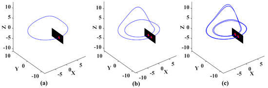
Figure 4.
Comparing the effect of changing the parameters values, used in Figure 3d, on number of Poincaré fixed points from left to right: (a) , (b) and (c) .
Poincaré section, in Figure 4a–c, tells that any change in the value of , or even leads the system to oscillate on a cyclic attractor of a certain period instead of chaos. Even if the change is slight as observed in the values of (from 0.2 to 0.1) and (from 0.2 to 0.5), which presents one and two Poincaré fixed points in Figure 4a and Figure 4b, respectively. In addition, the system becomes stable on a period-4 cycle (four Poincaré fixed points) rather than chaos (several Poincaré fixed points) when the parameter value is changed from 5.7 to 4.55 as shown in Figure 4c. It is evident now that each graph’s section contains a different number of Poincaré fixed points than those demonstrated in Figure 3d.
Thus, we observe in Figure 3a–d that as the number of red dots increases in the Poincaré section, the dynamical behavior becomes richer and more complex as the variations of the fractional-order , in the Rössler system (2), increase. This supports that the system can transition from low-period cycles to higher-period cycles (with one or few Poincaré fixed points) and eventually to chaotic dynamics (with dispersal Poincaré fixed points). Also, we have used the Poincaré section to show that detecting the dynamic behaviors caused by changing the parameter values of the Rössler system (2) is valid by observing the number of Poincaré fixed points.
In a nutshell, a hallmark of reflecting the system’s sensitivity to changes in the fractional-order and the parameters values is the observed change in the number of Poincaré fixed points, which indicates the emergence of new cyclic attractors of various periods and chaos. This confirms a significant result, which is that Poincaré sections can also be used in fractional-order systems to give a simpler visualization for the simple and complex dynamics.
To conclude this subsection, the Poincaré section offers a straightforward diagnostic method for visualizing and illustrating dynamic transitions, revealing how increasing the value of adds complexity to the behavior of the fractional-order Rössler system (2). Plus, It acts as an effective way to identify how altering the parameters values of the system impacts the dynamics.
A Poincaré fixed point is a point that allows the system to return to the same point on the section after one period, corresponding to a periodic orbit in the original system.
4.4. Lyapunov Exponents
Without a doubt, determining Lyapunov exponents is an essential tool for mathematicians to comprehend and recognize the stability and the emergence of chaos for any dynamical system. In other words, computing the Lyapunov spectrum characterizes the stability of the system (2). If all are negative, then the system’s dynamics converges to an equilibrium moving in a steadily stable manner. If one zero and the rest are negative, then the system oscillates stably in a periodic manner. The existence of at least one (two) positive suggests that the system behaves chaotically (hyper-chaotically), and hence one cannot predict the system’s behavior, as the system will have sensitive dependence on the initial conditions. Therefore, it is effective to track the system’s dynamics using the Lyapunov exponents when the fractional-order is varied.
Fixing the fractional-order at , as seen in Figure 5a, shows that there is not any positive sign for the three Lyapunov exponents , but zero and negative Lyapunov exponents are present. More specifically, the system has three Lyapunov exponents with one zero and two negatives, which dynamically indicates that the system behaves on a cyclic attractor. This result is in agreement with Figure 2 and Figure 3a, which confirms the stability of the system by oscillating in a cycle of period-1.
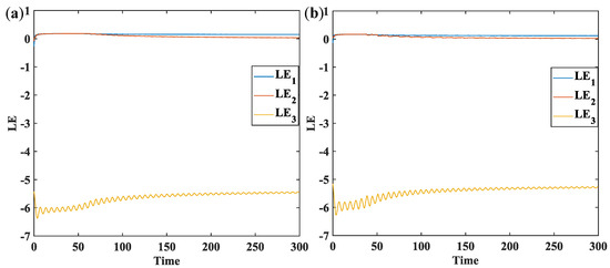
Figure 5.
The temporal evolution of Lyapunov exponents (LE1, LE2, LE3) at different values of the fractional-order in the system (2) from left to right: (a) and (b) .
Similarly, if the fractional-order is slightly increased to be (), the same signs of Lyapunov exponents show in Figure 5b (Figure 6a), which corresponds with regular dynamics repeating every two (four) time unit, namely the period-2 (period-4) cycle as already noticed in Figure 2 and emulated in Figure 3b (Figure 3c).
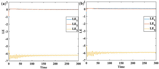
Figure 6.
The temporal evolution of Lyapunov exponents (LE1, LE2, LE3) at different values of the fractional-order in the system (2) from left to right: (a) and (b) .
By looking closely at Figure 6b, there are two positive signs for the first and second Lyapunov exponents, while the third Lyapunov exponent is negative. This confirms the emergence of hyper-chaos when as already exhibited in Figure 2 and Figure 3d, whereby the dynamic must have a highly sensitive dependence on the initial conditions.
All these simulations of the Lyapunov exponents at the four different values of the fractional-order are consistent with their corresponding dynamic behaviors presented in Figure 2 and Figure 3a–d. This confirms that the Rossler system (2) undergoes regular or chaotic motions depending on the value of the fractional-order. Plus, the temporal evolution of Lyapunov exponents (LE1, LE2, LE3), at , informs the dissipativity of the system dynamics because of their negative sum.
In chaos theory, Lyapunov exponents measure the degree of chaos in a system. A positive Lyapunov exponent indicates chaotic behavior; at least one positive exponent is needed to confirm chaos. A system is considered hyperchaotic if it satisfies two conditions: it has at least four dimensions (for autonomous systems), and it has two or more positive Lyapunov exponents, while the sum of all exponents remains negative. These conditions distinguish hyperchaotic systems as more complex than regular chaotic systems, providing richer dynamics. Due to this complexity, hyperchaotic systems are especially useful in applications like secure communications. Lyapunov exponents quantify a system’s chaos; at least one positive exponent indicates chaotic behavior for the fractional-order system: (0.0842, 0.0053, −6.4108) and (0.0981, 0.0071, −6.0542).
4.5. Chaos
This part of the study addresses the dynamic behaviors of system (1) under various fractional orders, parameter values, and demonstrates the creation of new chaotic attractors. Figure 7, Figure 8, Figure 9, Figure 10, Figure 11, Figure 12, Figure 13, Figure 14, Figure 15, Figure 16, Figure 17, Figure 18, Figure 19, Figure 20, Figure 21 and Figure 22 are phase portraits of the fractional-order system captured using the Equation (1), and the dynamical behavior of the system varies with variations in the fractional-order parameter and in the parameters of the system under different initial conditions. The classic case (), in Figure 7, presents a typical chaotic attractor structure, to which subsequent cases are referred. As is reduced slightly below 1, the system is still chaotic but undergoes extreme changes in the attractor geometry: more compressed, stretched, or asymmetric as the parameters are changed. Changing or tends to alter the spread and complexity of the attractor, while reducing tends to suppress chaotic dynamics or yields more periodic dynamics.
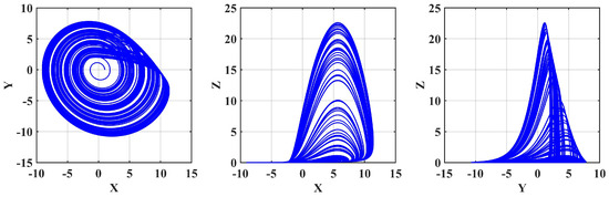
Figure 7.
System view (2) for and under I.Cs .
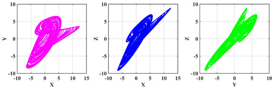
Figure 8.
System view (2) for and under I.Cs .
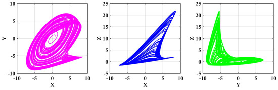
Figure 9.
System view (2) for and under I.Cs .
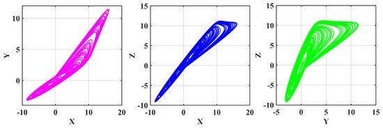
Figure 10.
System view (2) for and under I.Cs .
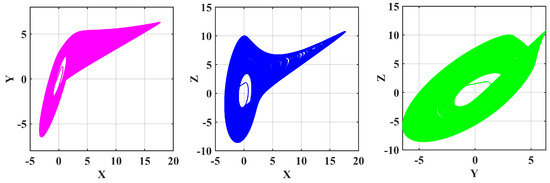
Figure 11.
System view (2) for and under I.Cs .
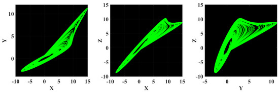
Figure 12.
System view (2) for and under I.Cs .
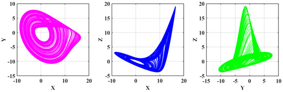
Figure 13.
System view (2) for and under I.Cs .
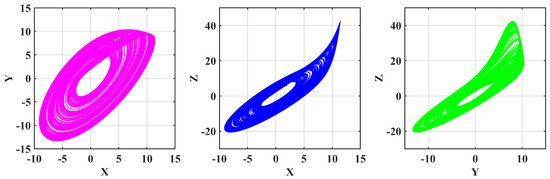
Figure 14.
System view (2) for and under I.Cs .
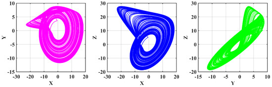
Figure 15.
System view (2) for and under I.Cs .
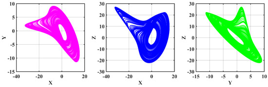
Figure 16.
System view (2) for and under I.Cs .
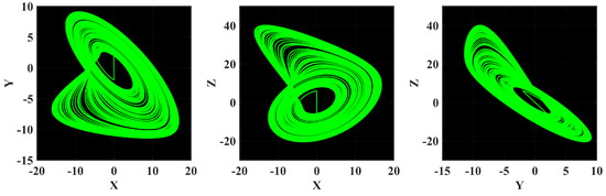
Figure 17.
System view (2) for and under I.Cs .
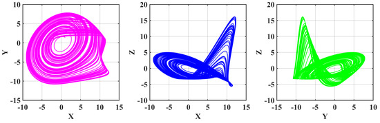
Figure 18.
System view (2) for and under I.Cs .
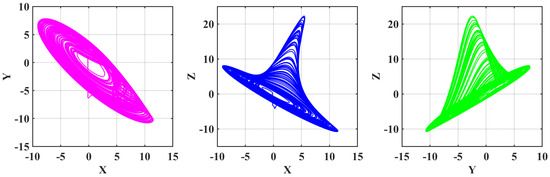
Figure 19.
System view (1) for and under I.Cs .
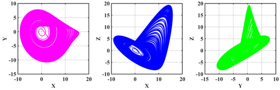
Figure 20.
System view (2) for and under I.Cs .
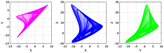
Figure 21.
System view (2) for and under I.Cs .
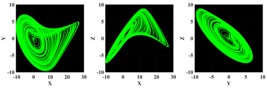
Figure 22.
System view (2) for and under I.Cs .
In addition, variations in the initial conditions affect the shape of the trajectory, which is sensitive to memory effects and parameter alterations. In general, the plots demonstrate the sensitive and rich dynamics that fractional-order systems allow, demonstrating their adaptability and usefulness in simulating complex behavior that ordinary integer-order counterparts are unable to account for.
Figure 12, Figure 17 and Figure 22 show unique chaotic attractors arising from different initial values (e.g., or ), unlike those reported in other studies. With altered parameter values (for example, smaller values or strongly symmetrical values of and ), new chaotic dynamics appear. Compared to the classical Lorenz-type attractors, the new structures are more irregular or asymmetric, indicating that the system is in a different regime of chaos.
4.6. Time Series
In this section, we study the dynamic behaviors of the Rossler system when there is a slight change in the fractional-order using time series plots. Although the Rössler system here is not designed to interpret a specific biological phenomenon, it is considered a very useful model in helping the mathematicians to understand, predict, and investigate its dynamic complexities in comparison with the resultant dynamics of other models such as cellular, chemical, and ecological systems.
The time series plots in Figure 23, Figure 24 and Figure 25 show the dynamic behaviors of the system’s states tested at different values of and with fixed constant parameters, namely . The system (1) is initialized at
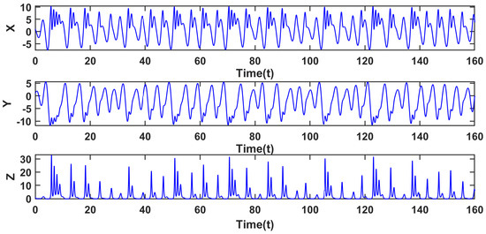
Figure 23.
Time series of system (2), including the transient dynamics, depicts chaotic behavior with highly irregular oscillations at .
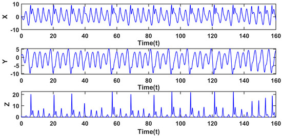
Figure 24.
Time series of system (2), including the transient dynamics, depicts chaotic behavior with less-irregular oscillations at .
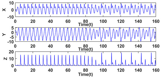
Figure 25.
Time series of system (2), including the transient dynamics, depicts two different stable behaviors shown as two types of regular oscillations, separated by dynamic transition, at .
In the classical case, when the fractional-order is fixed at , we find that the dynamic formation of chaos gives highly irregular oscillations as simulated in Figure 23. If the fractional-order value is changed to become as seen in Figure 24, the system (2) oscillates chaotically but exhibits noticeable changes in frequency and amplitude, which are a reflection of the memory effects caused by a decrease of , compared with Figure 23, in the fractional derivative. More precisely, the frequency and amplitude in the state variable Z is lower in Figure 24 in comparison with Figure 23. As a result of the system’s behavior changing over time, this proves that even if the percentage change of is relatively minuscule, the dynamics are highly sensitive to the value of the fractional-order . This biologically indicates that decreasing the memory effect has a positive influence on transitioning the complex behavior to less complex behavior that would appear if is decreased further provided that all the initial conditions are equal to one.
Following, Figure 25 informs that the system (2) oscillates with regular frequency and amplitude over the whole time scale if is fixed at . This confirms that decreasing the memory effect transitions the dynamics from complex case to less complex (regular). This confirms our implication that decreasing the fractional order further to leads to regular oscillations. More interestingly, the time series plot of Figure 25 contains two different types of behaviors, clearly seen in the first and second half. The first displays a periodic behavior repeating every two time units, while the second shows another regular dynamics with different frequency and amplitude representing a periodic behavior repeating every four time units. From a biological perspective, the existence of these dynamic transitions between two different periods over a time scale reflects how the dynamic behaviors switch between two distinct functional states in response to internal or external changes. One of these biological examples is predator–prey densities; the existence of such transitions biologically indicate that the two populations vary in two different patterns at a certain memory effect (if the studied predator–prey model is fractional).
A surprising fact here found is that the existence of dynamic transitions in the system (2) as observed in Figure 25 although the values of the fractional-order and parameters are fixed. The dynamic passes through a radical change in the behavior. This change is dynamically considered a transition from a regime to a different regime. Figure 26 closely illustrates that the dynamic starts oscillating at the beginning of the time scale until it stabilizes in a low-period regime and then moves to a higher-period regime after almost eighty units of time.
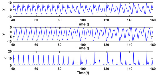
Figure 26.
Amplification of Figure 25 shows the dynamic transition from a low-period regime to a higher-period regime.
To sum up, it is remarkable that the sensitivity of the system’s dynamics to different values of the fractional-order becomes more pronounced, with oscillations showing more differences, which is a sign of either chaos or stability for the system (2). Plus, the fractional-order Rössler system can behave in two different behavioral modes (two attractors of different periods) based on the length of time. These results point out the significance of the fractional order in shaping the system’s behavior, specifically in increasing the complexity of the time-dependent response on time series plots.
5. Discussion
Dynamical systems are a major field of study that drives continuous work by researchers and professionals to create fractional-order models and analytical tools. Applied mathematics and fractional calculus, in particular, have been quite successful in capturing various intriguing dynamics.
Using the fractional Caputo differential operator inside a strong numerical framework, this paper offers a thorough examination of a nonlinear Rössler system of equations (Equation (1)). Focusing on its dynamic evolution and stability, we investigate the system behavior under different fractional orders, initial conditions, and parameters.
Our examined system, in this paper, is the Rössler system, which has been intensively studied to cover a spectrum of gaps that has not been investigated in the literature (see Table 1). We summarize all the covered gaps in terms of the previous studies in Table 1, which are as follows: fractional-order system (FDS), chaotic behavior (CH), non-chaotic regimes (NCH), symmetry analysis (SA), time series (TS), Lyapunov exponents (LE), bifurcations (BF), numerical simulation (NS), and Poincaré sections (PS). This confirms that we here cover the unexamined gaps in each study on the Rössler system when it is treated as a fractional-order model.
In the context of chaos emergence, extensive simulations are introduced in this part, supporting the emergence of chaos, where we show how new chaotic attractors can be created, and we analyze the dynamic behaviors of system (1) under different fractional orders, parameter values, and initial conditions. Phase portraits of the fractional-order system defined by system (1) are shown in Figure 7, Figure 8, Figure 9, Figure 10, Figure 11, Figure 12, Figure 13, Figure 14, Figure 15, Figure 16, Figure 17, Figure 18, Figure 19, Figure 20, Figure 21 and Figure 22. They also show how the dynamical behavior of the system changes as the fractional-order parameter and the system parameters (A1, A2, and A3) change under various initial conditions. Subsequent cases are related to the classic case () in Figure 7, which displays a typical chaotic attractor structure. This is a clear sign of chaos emergence in the Rössler system, whether in the classical case () or the fractional case ().
The section on time series introduces sophisticated simulations, as shown in Figure 23, Figure 24, Figure 25 and Figure 26, that demonstrate how the dynamic behaviors of system (1) appear over various time scales under different fractional orders. We also examine how the Rössler system’s dynamics can have sensitivity to dynamics. This reveals that the fractional-order parameter , which controls the system’s memory and inheritance effects, can cause the system to show considerable sensitivity. The system’s stability and dynamic behavior can all be significantly impacted by small changes to this control parameter.
The description of dynamics in Figure 2 is associated with studying bifurcations, which arises in Section 4.2, discussed deeply when the fractional-order undergoes increasing variations, namely . Throughout the analysis of 1D bifurcation, we find the fact that the periods of cyclic attractors double with the increase in the fractional-order parameter. Also, this section leads to another fact that chaos can take place in a route of cascade of period-doublings before the system (1) satisfies the classical case.
The discussion of Poincaré sections and Lyapunov exponents is then covered in detail, with Figure 3a–d, Figure 5a,b, and Figure 6a,b simulating the key plots. In both sections, we show that chaos can be detected in two different methods: Poincaré sections and Lyapunov exponents. However, we exhibit how Poincaré fixed points on the black sections can be used to reflect regular period dynamics, such as one, two, and four. Accordingly, the results are valid and accurate because they are compatible with the signs of the three Lyapunov exponents.
Future studies might address the consequences of fractional-order derivatives for stability and bifurcation structures, thus improving the knowledge of other nonlinear systems. For example, the Lorenz system can be used to study how fractional-order derivatives affect the system’s stability and dynamic behaviors.
We know that fixing the initialization problem in fractional-order systems is very important since it has a great effect on how they behave over time. The Caputo derivative is popular because it works well with classical initial conditions and is useful for modeling and simulation, especially when there is no pre-initial history. However, it does not fully capture the memory and non-local effects that are unique to fractional dynamics. Earlier publications have shown this limitation using diffusive representations and infinite-dimensional state-space models. These models reveal that Caputo-type initializations correspond to pseudo-state variables instead of actual states in the classical sense. We chose the Caputo formulation for this study since it is useful in real life, but we know that we need more strict initialization frameworks. In the future, we will examine other definitions, like Riemann–Liouville and Grünwald–Letnikov derivatives, and we will also engage in developing initialization procedures that account for the system’s entire memory. The aim of these efforts is to bridge the gap between pseudo-states and real states and to reduce errors that are a consequence of normal initialization. This will render the long-term simulation and control of fractional-order systems more reliable. Our work is grounded in known initial conditions, but its main contribution is that it uncovers novel and intricate dynamic phenomena, like novel chaotic attractors and memory-dependent patterns. This is a demonstration of how fractional-order models differ from integer-order models.
Although we here have introduced a variety of dynamic behaviors, there are still some limitations that have not been explored yet in this work. For example, this presented work is only focused on the case whereby the fractional-order of the three variables varies equally and simultaneously, while one can also study the case whereby two or three fractional-orders vary differently using a more suitable numerical method. This would be much harder but possible if we think that emulating the variations of the fractional-orders combines in a 2D or 3D bifurcation diagram, reflecting the overall dynamic behavior of the Rossler system. Its implementation would lead to exploring more interesting dynamics never discussed in systems having different fractional orders, including catastrophe, hysteresis, reversibility, and irreversibility.
6. Conclusions
The current work has shown a highly precise numerical method for fractional-order chaotic system analysis with significant improvements over traditional methods. The method has been revealed with extensive simulations to be capable of reproducing complex dynamic behaviors, including new chaos, strange attractors, and rich time series patterns, that were not observed using traditional methods. One of the interesting findings is that the analysis of time series gives evidence that lowering not only leads to changes in the dynamics of the system over time, but it also allows the existence of dynamic transitions in the Rössler system (2) when its order is fractional. The results clearly demonstrate that parameters and initial conditions strongly influence the decision of the qualitative nature of the system dynamics and therefore indicate the necessity of the consideration of fractional effects in models of real processes. Applying sophisticated diagnostic tools such as Poincaré sections, Lyapunov exponents, and bifurcation analysis, we have carried out a stringent study of the stability, transitions, and geometric structure of the system. These analyses attest that the method we suggest not only compares with the traditional integer-order methods in those applications where they are valid but even surpasses them significantly in accuracy as well as the ability to uncover hidden, subtle fractional behavior that even they cannot discern. In addition, the findings confirm the necessity of designing special numerical algorithms for fractional-order systems due to the incapability of conventional approaches to express all the intricacies of such models. The superior efficiency, accuracy, and precision of the presented method make it a productive tool for scientists who investigate complex, memory-based, and hereditary systems in a wide range of scientific and engineering disciplines. In the future, we aim to solve new fractional models [44], and compare with other methods [45].
Author Contributions
Methodology, R.A., A.S., M.A.A., F.J.A., M.B. and S.A.A.; Validation, R.A., A.S., M.A.A., F.J.A., M.B. and S.A.A.; Formal analysis, R.A., A.S., M.A.A., F.J.A., M.B. and S.A.A.; Investigation, R.A., A.S., M.A.A., F.J.A., M.B. and S.A.A.; Writing—original draft, R.A., A.S., M.A.A., F.J.A., M.B. and S.A.A.; Writing—review and editing, R.A., A.S., M.A.A., F.J.A., M.B. and S.A.A. All authors have read and agreed to the published version of the manuscript.
Funding
This research received no external funding.
Data Availability Statement
The original contributions presented in this study are included in the article.
Conflicts of Interest
The authors declare that there are no conflicts of interest regarding the publication of this article.
References
- Saadeh, R.; Abdoon, M.A.; Qazza, A.; Berir, M.; Guma, F.E.; Al-Kuleab, N.; Degoot, A.M. Mathematical modeling and stability analysis of the novel fractional model in the Caputo derivative operator: A case study. Heliyon 2024, 10, e26611. [Google Scholar] [CrossRef]
- Abdoon, M.A.; Alzahrani, A.B. Comparative analysis of influenza modeling using novel fractional operators with real data. Symmetry 2024, 16, 1126. [Google Scholar] [CrossRef]
- Hilfer, R. Applications of Fractional Calculus in Physics; World Scientific: Singapore, 2000. [Google Scholar]
- Gündoǧdu, H.; Joshi, H. Numerical analysis of time-fractional cancer models with different types of net killing rate. Mathematics 2025, 13, 536. [Google Scholar] [CrossRef]
- Ferrari, A.L.; Gomes, M.C.S.; Aranha, A.C.R.; Paschoal, S.M.; de Souza Matias, G.; de Matos Jorge, L.M.; Defendi, R.O. Mathematical modeling by fractional calculus applied to separation processes. Sep. Purif. Technol. 2024, 337, 126310. [Google Scholar] [CrossRef]
- Zehra, A.; Naik, P.A.; Hasan, A.; Farman, M.; Nisar, K.S.; Chaudhry, F.; Huang, Z. Physiological and chaos effect on dynamics of neurological disorder with memory effect of fractional operator: A mathematical study. Comput. Methods Programs Biomed. 2024, 250, 108190. [Google Scholar] [CrossRef]
- Naik, P.A.; Yavuz, M.; Qureshi, S.; Owolabi, K.M.; Soomro, A.; Ganie, A.H. Memory impacts in hepatitis C: A global analysis of a fractional-order model with an effective treatment. Comput. Methods Programs Biomed. 2024, 254, 108306. [Google Scholar] [CrossRef]
- Santra, P.; Induchoodan, R.; Mahapatra, G. Analyzing election trends incorporating memory effect through a fractional-order mathematical modeling. Phys. Scr. 2024, 99, 075239. [Google Scholar] [CrossRef]
- Golbabai, A.; Nikan, O.; Nikazad, T. Numerical investigation of the time fractional mobile-immobile advection-dispersion model arising from solute transport in porous media. Int. J. Appl. Comput. Math. 2019, 5, 50. [Google Scholar] [CrossRef]
- Maayaha, B.; Bushnaqb, S.; Moussaouia, A. Numerical solution of fractional order SIR model of dengue fever disease via Laplace optimized decomposition method. J. Math. Comput. Sci. 2024, 32, 86–93. [Google Scholar] [CrossRef]
- Hammouch, Z.; Mekkaoui, T. Traveling-wave solutions of the generalized Zakharov equation with time-space fractional derivatives. Math. Eng. Sci. Aerosp. MESA 2014, 5, 1–11. [Google Scholar]
- Toufik, M.; Atangana, A. New numerical approximation of fractional derivative with non-local and non-singular kernel: Application to chaotic models. Eur. Phys. J. Plus 2017, 132, 444. [Google Scholar] [CrossRef]
- Amiri, Z.; Heidari, A.; Jafari, N.; Hosseinzadeh, M. Deep study on autonomous learning techniques for complex pattern recognition in interconnected information systems. Comput. Sci. Rev. 2024, 54, 100666. [Google Scholar] [CrossRef]
- Liu, L.; Wan, L. Innovative models for enhanced student adaptability and performance in educational environments. PLoS ONE 2024, 19, e0307221. [Google Scholar] [CrossRef] [PubMed]
- Rane, J.; Mallick, S.; Kaya, O.; Rane, N. Scalable and adaptive deep learning algorithms for large-scale machine learning systems. Future Res. Oppor. Artif. Intell. Ind. 2024, 4, 39–92. [Google Scholar]
- Shyaa, M.A.; Ibrahim, N.F.; Zainol, Z.; Abdullah, R.; Anbar, M.; Alzubaidi, L. Evolving cybersecurity frontiers: A comprehensive survey on concept drift and feature dynamics aware machine and deep learning in intrusion detection systems. Eng. Appl. Artif. Intell. 2024, 137, 109143. [Google Scholar] [CrossRef]
- Usman, M.; Makinde, O.D.; Khan, Z.H.; Ahmad, R.; Khan, W.A. Applications of fractional calculus to thermodynamics analysis of hydromagnetic convection in a channel. Int. Commun. Heat Mass Transf. 2023, 149, 107105. [Google Scholar] [CrossRef]
- Barbero, G.; Evangelista, L.R.; Zola, R.S.; Lenzi, E.K.; Scarfone, A. A Brief Review of Fractional Calculus as a Tool for Applications in Physics: Adsorption Phenomena and Electrical Impedance in Complex Fluids. Fractal Fract. 2024, 8, 369. [Google Scholar] [CrossRef]
- Elbadri, M.; Abdoon, M.A.; Berir, M.; Almutairi, D.K. A symmetry chaotic model with fractional derivative order via two different methods. Symmetry 2023, 15, 1151. [Google Scholar] [CrossRef]
- Vieira, L.C.; Costa, R.S.; Valério, D. An overview of mathematical modelling in cancer research: Fractional calculus as modelling tool. Fractal Fract. 2023, 7, 595. [Google Scholar] [CrossRef]
- Padder, A.; Almutairi, L.; Qureshi, S.; Soomro, A.; Afroz, A.; Hincal, E.; Tassaddiq, A. Dynamical analysis of generalized tumor model with Caputo fractional-order derivative. Fractal Fract. 2023, 7, 258. [Google Scholar] [CrossRef]
- Berir, M. A fractional study for solving the smoking model and the chaotic engineering model. In Proceedings of the 2023 2nd International Engineering Conference on Electrical, Energy, and Artificial Intelligence (EICEEAI), Zarqa, Jordan, 27–28 December 2023; pp. 1–6. [Google Scholar]
- Pelton, S.I.; Mould-Quevedo, J.F.; Nguyen, V.H. The impact of adjuvanted influenza vaccine on disease severity in the US: A stochastic model. Vaccines 2023, 11, 1525. [Google Scholar] [CrossRef]
- Qureshi, S. Real life application of Caputo fractional derivative for measles epidemiological autonomous dynamical system. Chaos Solitons Fractals 2020, 134, 109744. [Google Scholar] [CrossRef]
- Olayiwola, M.O.; Yunus, A.O. Mathematical analysis of a within-host dengue virus dynamics model with adaptive immunity using Caputo fractional-order derivatives. J. Umm-Qura Univ. Appl. Sci. 2025, 11, 104–123. [Google Scholar] [CrossRef]
- Rössler, O.E. An equation for continuous chaos. Phys. Lett. A 1976, 57, 397–398. [Google Scholar] [CrossRef]
- Zhang, W.; Zhou, S.; Li, H.; Zhu, H. Chaos in a fractional-order Rössler system. Chaos Solitons Fractals 2009, 42, 1684–1691. [Google Scholar] [CrossRef]
- Rysak, A.; Sedlmayr, M.; Gregorczyk, M. Revealing fractionality in the Rössler system by recurrence quantification analysis. Eur. Phys. J. Spec. Top. 2023, 232, 83–98. [Google Scholar] [CrossRef]
- Čermák, J.; Nechvátal, L. Local bifurcations and chaos in the fractional Rössler system. Int. J. Bifurc. Chaos 2018, 28, 1850098. [Google Scholar] [CrossRef]
- Letellier, C.; Aguirre, L.A. Dynamical analysis of fractional-order Rössler and modified Lorenz systems. Phys. Lett. A 2013, 377, 1707–1719. [Google Scholar] [CrossRef]
- Li, C.; Chen, G. Chaos and hyperchaos in the fractional-order Rössler equations. Phys. A Stat. Mech. Its Appl. 2004, 341, 55–61. [Google Scholar] [CrossRef]
- Cafagna, D.; Grassi, G. Hyperchaos in the fractional-order Rössler system with lowest-order. Int. J. Bifurc. Chaos 2009, 19, 339–347. [Google Scholar] [CrossRef]
- Li, Z.; Chen, D.; Ma, M.; Zhang, X.; Wu, Y. Feigenbaum’s constants in reverse bifurcation of fractional-order Rössler system. Chaos Solitons Fractals 2017, 99, 116–123. [Google Scholar] [CrossRef]
- Sulaiman, I.M.; Owoyemi, A.E.; Nawi, M.A.A.; Muhammad, S.S.; Muhammad, U.; Jameel, A.F.; Nawawi, M.K.M. Stability and Bifurcation Analysis of Rössler System in Fractional Order. In Proceedings of the Advances in Intelligent Manufacturing and Mechatronics: Selected Articles from the Innovative Manufacturing, Mechatronics & Materials Forum (iM3F 2022), Pahang, Malaysia, 26–27 July 2022; pp. 239–250. [Google Scholar]
- Aguila-Camacho, N.; Duarte-Mermoud, M.A.; Gallegos, J.A. Lyapunov functions for fractional order systems. Commun. Nonlinear Sci. Numer. Simul. 2014, 19, 2951–2957. [Google Scholar] [CrossRef]
- Rayal, A.; Dogra, P.; Thabet, S.T.; Kedim, I.; Vivas-Cortez, M. A Numerical Study of the Caputo Fractional Nonlinear Rössler Attractor Model via Ultraspherical Wavelets Approach. Comput. Model. Eng. Sci. 2025, 143, 1895–1925. [Google Scholar] [CrossRef]
- Barrio, R.; Blesa, F.; Serrano, S. Qualitative analysis of the Rössler equations: Bifurcations of limit cycles and chaotic attractors. Phys. D Nonlinear Phenom. 2009, 238, 1087–1100. [Google Scholar] [CrossRef]
- Maheri, M.; Arifin, N.M. Synchronization of two different fractional-order chaotic systems with unknown parameters using a robust adaptive nonlinear controller. Nonlinear Dyn. 2016, 85, 825–838. [Google Scholar] [CrossRef]
- Wang, J.L.; Wang, Y.L.; Li, X.Y. An efficient numerical simulation of chaos dynamical behaviors for fractional-order Rössler chaotic systems with Caputo fractional derivative. J. Low Freq. Noise Vib. Act. Control 2024, 43, 609–616. [Google Scholar] [CrossRef]
- Petráš, I. Fractional-order chaotic systems. In Fractional-Order Nonlinear Systems: Modeling, Analysis and Simulation; Springer: Berlin/Heidelberg, Germany, 2021; pp. 103–184. [Google Scholar]
- Diethelm, K.; Ford, N. The Analysis of Fractional Differential Equations; Lecture notes in mathematics; Springer: Berlin/Heidelberg, Germany, 2010; Volume 2004. [Google Scholar]
- Tavazoei, M.S. Fractional order chaotic systems: History, achievements, applications, and future challenges. Eur. Phys. J. Spec. Top. 2020, 229, 887–904. [Google Scholar] [CrossRef]
- Podlubny, I. Fractional Differential Equations; Academic Press: San Diego, CA, USA, 1999. [Google Scholar]
- Thabet, S.T.; Kedim, I.; Abdalla, B.; Abdeljawad, T. The q-analogues of nonsingular fractional operators with Mittag-Leffler and exponential kernels. Fractals 2024, 32, 2440044. [Google Scholar] [CrossRef]
- Eltayeb, H.; Elgezouli, D.E. A Note on Fractional Third-Order Partial Differential Equations and the Generalized Laplace Transform Decomposition Method. Fractal Fract. 2024, 8, 602. [Google Scholar] [CrossRef]


Disclaimer/Publisher’s Note: The statements, opinions and data contained in all publications are solely those of the individual author(s) and contributor(s) and not of MDPI and/or the editor(s). MDPI and/or the editor(s) disclaim responsibility for any injury to people or property resulting from any ideas, methods, instructions or products referred to in the content. |
© 2025 by the authors. Licensee MDPI, Basel, Switzerland. This article is an open access article distributed under the terms and conditions of the Creative Commons Attribution (CC BY) license (https://creativecommons.org/licenses/by/4.0/).