Article

Composite Estimators for the Population Mean Under Ranked Set Sampling

Department of Mathematics & Statistics, North Carolina A&T State University, Greensboro, NC 27411, USA
*
Author to whom correspondence should be addressed.
Mathematics 2025, 13(19), 3071; https://doi.org/10.3390/math13193071
Submission received: 22 July 2025 / Revised: 17 September 2025 / Accepted: 19 September 2025 / Published: 24 September 2025
(This article belongs to the Special Issue Innovations in Survey Statistics and Survey Sampling)

Abstract

Ranked Set Sampling (RSS) is an effective sampling technique, particularly when precise measurement of the study variable is costly or time-consuming, but ranking the units is relatively easy. Estimation of the finite population mean from RSS, with and without auxiliary information, has been widely studied, with estimators such as the RSS sample mean, ratio estimator, and regression estimators receiving considerable attention. While the RSS sample mean does not utilize auxiliary information, the ratio and regression estimators rely heavily on its quality. To address these limitations, this study proposes a shrinkage-type (composite) estimator for the finite population mean. The proposed estimator adaptively combines the RSS sample mean and the ratio estimator, leveraging auxiliary information when it is useful while maintaining robustness when it is not. We derive its statistical properties, including bias, variance, and mean squared error. Simulation studies demonstrate that the proposed estimator can outperform conventional estimators across a range of scenarios. We illustrate the method through a real data application.

1. Introduction

Efficient sampling methods are essential in statistical analysis, especially when acquiring data is costly or time-consuming. In such contexts, alternative sampling designs that leverage auxiliary information or partial measurements can offer significant advantages. One such approach is Ranked Set Sampling (RSS), first introduced by McIntyre [1] in the early 1950s to estimate pasture yields in Australia. Since its inception, RSS has gained considerable attention due to its ability to increase estimation efficiency with minimal additional cost or effort, particularly in environments where precise measurement is costly, but ranking units is relatively easy [2]. RSS has been successfully applied in a variety of fields—including agriculture, environmental science, and economics—where it has outperformed Simple Random Sampling (SRS) in estimation efficiency.
To implement RSS, a total of p 2 units are randomly selected from the population and divided into p sets, each containing p units. Within each set, the units are ranked based on visual inspection, expert judgment, concomitant variables, or other means that do not involve precise quantification. The process continues as follows: the smallest unit from the first set is measured, the second smallest unit from the second set is measured, and so forth, until the largest unit from the p-th set is measured. This procedure constitutes a single cycle of RSS, which can be repeated for m independent cycles to obtain a balanced RSS of size n = p m : { Y [ k ] l : k = 1 , 2 , , p ; l = 1 , 2 , , m } , where Y [ k ] l denotes the k-th judgment order statistic of the units in the k-th set of the l-th cycle. The use of square brackets instead of parentheses signifies that ranking may be subject to error or imperfection. If ranking is perfect, the notation Y ( k ) l may be used instead.
To illustrate the technique, in a balanced RSS with p = 4 and m = 2 , with ranking based on an auxiliary (or concomitant) variable X, the selection proceeds as follows:
  • Cycle 1:
    X ( 1 ) 1 X ( 2 ) 1 X ( 3 ) 1 X ( 4 ) 1 ( X ( 1 ) 1 , Y [ 1 ] 1 ) X ( 1 ) 1 X ( 2 ) 1 X ( 3 ) 1 X ( 4 ) 1 ( X ( 2 ) 1 , Y [ 2 ] 1 ) X ( 1 ) 1 X ( 2 ) 1 X ( 3 ) 1 X ( 4 ) 1 ( X ( 3 ) 1 , Y [ 3 ] 1 ) X ( 1 ) 1 X ( 2 ) 1 X ( 3 ) 1 X ( 4 ) 1 ( X ( 4 ) 1 , Y [ 4 ] 1 )
  • Cycle 2:
    X ( 1 ) 2 X ( 2 ) 2 X ( 3 ) 2 X ( 4 ) 2 ( X ( 1 ) 2 , Y [ 1 ] 2 ) X ( 1 ) 2 X ( 2 ) 2 X ( 3 ) 2 X ( 4 ) 2 ( X ( 2 ) 2 , Y [ 2 ] 2 ) X ( 1 ) 2 X ( 2 ) 2 X ( 3 ) 2 X ( 4 ) 2 ( X ( 3 ) 2 , Y [ 3 ] 2 ) X ( 1 ) 2 X ( 2 ) 2 X ( 3 ) 2 X ( 4 ) 2 ( X ( 4 ) 2 , Y [ 4 ] 2 )
    producing a balanced RSS:
    s = ( X ( 1 ) 1 , Y [ 1 ] 1 ) , ( X ( 2 ) 1 , Y [ 2 ] 1 ) , ( X ( 3 ) 1 , Y [ 3 ] 1 ) , ( X ( 4 ) 1 , Y [ 4 ] 1 ) , ( X ( 1 ) 2 , Y [ 1 ] 2 ) , ( X ( 2 ) 2 , Y [ 2 ] 2 ) , ( X ( 3 ) 2 , Y [ 3 ] 2 ) , ( X ( 4 ) 2 , Y [ 4 ] 2 ) .
There is a vast body of literature on statistical inference using RSS, including parametric estimation of population parameters such as the mean (e.g., [3]), variance (e.g., [4]), and quantiles (e.g., [5]), and nonparametric estimation and hypothesis testing (e.g., [6,7,8,9,10]). For a comprehensive review, see [11].
In this paper, we consider the problem of estimating a finite population mean using RSS. Let U = { 1 , 2 , , N } denote a finite population of size N, where each unit i U is associated with a value y i of a study variable Y, and a value x i of an auxiliary variable X. The parameter of interest is the finite population mean:
Y ¯ = 1 N i = 1 N y i .
The goal is to estimate Y ¯ based on an RSS of size n. Numerous estimators have been proposed for this purpose, including the simple mean of the RSS ([12]), the ratio estimator ([13,14]), and the regression estimator ([15]).
In this study, we propose a shrinkage-type (composite) estimator for estimating the finite population mean in the context of RSS. This estimator builds upon the idea of combining two or more estimators using shrinkage weights, offering a compromise that can outperform the individual components under certain conditions. Specifically, we extend the work of Lui [16], who proposed a composite estimator that blends the simple mean and the ratio estimator under SRS. Lui [16] showed that the composite approach can offer improved performance when certain conditions are met. Their simulation study suggested that the SRS composite estimator could outperform the simple and ratio estimators individually, especially when the auxiliary variable is moderately to strongly correlated with the study variable. We extend and study this idea under RSS. We provide theoretical results that characterize the performance of the proposed estimator and explore its properties through simulation and real data analysis.
The remainder of this paper is organized as follows. Section 2 reviews the idea of composite estimators under SRS. Section 3 introduces the proposed composite estimator under RSS and derives its theoretical properties. Section 4 presents a simulation study investigating the finite sample performance of the proposed estimator relative to several other estimators. Section 5 illustrates the performance of the proposed estimator on a real dataset. Section 6 concludes the paper with a discussion of key findings and future research directions.

2. Composite Estimators Under SRS

In this section, we review the idea of composite estimators under SRS. The simplest estimator for the finite population mean under SRS is the simple mean estimator defined by [12]:
y ¯ SRS = 1 n i = 1 n y i .
The simple mean estimator is known to be unbiased and its variance, or, equivalently, its mean squared error (MSE), is given by [12], ch. 2:
MSE ( y ¯ SRS ) = Var ( y ¯ SRS ) = 1 n N S y 2 n ,
where S y 2 = 1 N 1 i = 1 N ( y i Y ¯ ) 2 is the variance of the study variable Y.
An alternative estimator that is commonly used to take advantage of available auxiliary information is the ratio estimator, which is defined as follows under SRS [12]:
y ¯ rSRS = y ¯ SRS x ¯ SRS X ¯ .
The approximate variance of the ratio estimator under SRS is given by [12], ch. 6:
Var ( y ¯ rSRS ) 1 n N 1 n [ S y 2 + R 2 S x 2 2 R S x y ] = 1 n N 1 n Y ¯ 2 [ C y 2 + C x 2 2 ρ C x C y ] .
where R = Y ¯ X , S x y = 1 N 1 i = 1 N ( x i X ¯ ) ( y i Y ¯ ) , C z 2 = S z 2 Z 2 is the squared population coefficient of variation of a generic variable Z, and ρ = S x y S x S y is the population Pearson’s correlation coefficient between X and Y. Under SRS, Lui [16] suggested combining the simple mean estimator and the ratio estimator into a composite estimator defined by
y ¯ cSRS = w y ¯ SRS + ( 1 w ) y ¯ rSRS ,
where 0 w 1 is an unknown weight parameter. Observing the fact that, since y ¯ SRS is unbiased,
| Bias ( y ¯ cSRS ) | = | E ( y ¯ cSRS Y ¯ ) | = | ( 1 w ) E ( y ¯ rSRS Y ¯ ) | | E ( y ¯ rSRS Y ¯ ) | = | Bias ( y ¯ rSRS ) |
and the fact that the ratio estimator under SRS is asymptotically unbiased, ref. [16] derived the optimal weight by minimizing the variance of the composite estimator:
w SRS * = Var ( y ¯ rSRS ) Cov ( y ¯ SRS , y ¯ rSRS ) Var ( y ¯ rSRS ) + Var ( y ¯ SRS ) 2 Cov ( y ¯ SRS , y ¯ rSRS ) = 1 ρ C y / C x ,
where Cov ( U , V ) = E [ ( U E ( U ) ) ( V E ( V ) ) ] . According to Lui [16], there are specific circumstances in which the composite estimator surpasses the ratio estimator under SRS. These conditions are related to the correlation between X and Y, as well as their coefficients of variation. In addition, a simulation study was carried out by Lui [16] to showcase the efficiency of the composite estimator compared to the simple mean estimator and the ratio estimator under SRS. In this study, we are building upon the research conducted by [16] and expanding it to the context of RSS. In the following section, we will review the existing estimators for the population mean under RSS and introduce our proposed composite estimator.

3. Composite Estimators Under RSS

3.1. SimpleMean Estimator Under RSS

The unbiased mean estimator under RSS is given by
y ¯ RSS = 1 p m k = 1 p l = 1 m y [ k ] l .
Under RSS, the MSE of y ¯ RSS is given by Samawi and Muttlak [13] as follows:
MSE ( y ¯ RSS ) = 1 p m S y 2 1 p k = 1 p τ y [ k ] 2 ,
where τ y [ k ] = ( μ y [ k ] Y ¯ ) , with μ y [ k ] being the mean of the k-th order statistic of the study variable.

3.2. Ratio Estimator Under RSS

The conventional ratio estimator for the population mean Y ¯ of the study variable, y, is established as a quotient of two auxiliary variables, namely, the total of the study variable in the sample and the corresponding total of a related variable in the population. This estimator is widely used in various research fields, including business and academia, as it provides a reliable and efficient approach for estimating population means.
The ratio estimator under RSS is given by
y ¯ rRSS = y ¯ RSS x ¯ RSS X ¯ ,
where
x ¯ RSS = 1 p m k = 1 p l = 1 m x ( k ) l .
First-order approximations––assuming a large n = p m ––of the bias and MSE of the ratio estimator in Equation (5) are given by Kadilar et al. [14]:
Bias ( y ¯ rRSS ) Y ¯ 1 p m ( C x 2 C y x ) ( W x 2 W y x ) ,
MSE ( y ¯ rRSS ) 1 p m S y 2 2 R S x y + R 2 S x 2 1 p 2 m k = 1 p τ y [ k ] 2 2 R k = 1 p τ y x ( k ) + R 2 k = 1 p τ x ( k ) 2 ,
where
C y x = ρ C y C x = S x y Y ¯ X ¯ , W x 2 = 1 p 2 m X ¯ 2 k = 1 p τ x ( k ) 2 , and W y x = 1 p 2 m X ¯ Y ¯ k = 1 p τ y x ( k ) ,
with
τ x ( k ) = ( μ x ( k ) X ¯ ) , τ y x ( k ) = ( μ x ( k ) X ¯ ) ( μ y [ k ] Y ¯ ) , μ x ( k ) = E ( X ( k ) ) , and μ y [ k ] = E ( Y [ k ] ) .

3.3. Proposed Composite Estimator

In this study, we propose the use of a composite estimator, which is defined as a mixture of the simple mean estimator and the ratio estimator, for estimating the finite population mean Y ¯ under RSS. The estimator is defined as follows:
y ¯ ¨ cRSS = w y ¯ RSS + ( 1 w ) y ¯ rRSS ,
where 0 w 1 represents an unknown weight parameter. To derive the statistical properties of this estimator, we assume w to be fixed, and hence the use of the dot notation in y ¯ ¨ cRSS . Later in this section, we will derive the optimal weight and propose a corresponding estimator.
The following theorem and corollary summarize the statistical properties of the composite estimator in (8).
Theorem 1.
Under RSS, first-order approximations of the design-bias and variance of the composite estimator y ¯ ¨ cRSS are given by
Bias ( y ¯ ¨ cRSS ) = ( 1 w ) Bias ( y ¯ rRSS ) ( 1 w ) Y ¯ 1 p m ( C x 2 C y x ) ( W x 2 W y x )
and
Var ( y ¯ ¨ cRSS ) w 2 A + ( 1 w ) 2 B + 2 w ( 1 w ) C ,
where
A : = Var ( y ¯ R S S ) = 1 p m S y 2 1 p k = 1 p τ y [ k ] 2 ,
B : = Var ( y ¯ r R S S ) 1 p m S y 2 2 R S y x + R 2 S x 2 1 p 2 m k = 1 p τ y [ k ] 2 2 R k = 1 p τ y x ( k ) + R 2 k = 1 p τ x ( k ) 2 Y ¯ 2 1 p m ( C x 2 C y x ) W x 2 W y x 2
and
C : = Cov ( y ¯ R S S , y ¯ r R S S ) = 1 p m S y 2 1 p k = 1 p τ y [ k ] 2 R 1 p m S y x 2 1 p k = 1 p τ y x ( k ) 2 .
Proof. 
We start with the bias statement. First, notice that
E ( y ¯ ¨ cRSS ) = w E ( y ¯ RSS ) + ( 1 w ) E ( y ¯ rRSS ) = w Y ¯ + ( 1 w ) E ( y ¯ rRSS ) .
Therefore,
Bias ( y ¯ ¨ cRSS ) = E ( y ¯ ¨ cRSS ) Y ¯ = w Y ¯ + ( 1 w ) E ( y ¯ rRSS ) ( w Y ¯ + ( 1 w ) Y ¯ ) = ( 1 w ) E ( y ¯ rRSS ) Y ¯ = ( 1 w ) Bias ( y ¯ rRSS ) ( 1 w ) Y ¯ 1 p m ( C x 2 C y x ) ( W x 2 W y x ) ,
where the last equality follows from Equation (6).
Next, we derive the variance statement. Observe that
Var ( y ¯ ¨ cRSS ) = w 2 Var ( y ¯ RSS ) + ( 1 w ) 2 Var ( y ¯ rRSS ) + 2 w ( 1 w ) Cov ( y ¯ RSS , y ¯ rRSS ) = w 2 A + ( 1 w ) 2 B + 2 w ( 1 w ) C .
Now, A in Equation (11) follows directly from Equation (4), whereas B in Equation (12) follows from combining Equations (6) and (7) into B = Var ( y ¯ rRSS ) = MSE ( y ¯ rRSS ) Bias 2 ( y ¯ rRSS ) . Finally,
C = Cov ( y ¯ RSS , y ¯ rRSS ) = E ( y ¯ RSS Y ¯ ) ( y ¯ rRSS Y ¯ ) = E ( y ¯ RSS Y ¯ ) y ¯ RSS x ¯ RSS X ¯ Y ¯ = E ( y ¯ RSS Y ¯ ) X ¯ x ¯ RSS y ¯ RSS Y ¯ X ¯ x ¯ RSS E ( y ¯ RSS Y ¯ ) · 1 · y ¯ RSS R x ¯ RSS = E ( y ¯ RSS Y ¯ ) { y ¯ RSS Y ¯ } R { x ¯ RSS X ¯ } = E ( y ¯ RSS Y ¯ ) 2 E R ( x ¯ RSS X ¯ ) ( y ¯ RSS Y ¯ ) = Var ( y ¯ RSS ) R Cov ( x ¯ RSS , y ¯ RSS ) = 1 p m S y 2 1 p k = 1 p τ y [ k ] 2 R 1 p m S y x 2 1 p k = 1 p τ y x ( k ) 2 .
The proof is complete. □
Corollary 1.
Under RSS, the first-order approximation of the MSE of the composite estimator y ¯ ¨ cRSS is given by
MSE ( y ¯ ¨ cRSS ) w 2 1 p m S y 2 1 p k = 1 p τ y [ k ] 2 + ( 1 w ) 2 [ 1 p m S y 2 2 R S y x + R 2 S x 2 1 p 2 m k = 1 p τ y [ k ] 2 2 R k = 1 p τ y x ( k ) + R 2 k = 1 p τ x ( k ) 2 ] + 2 w ( 1 w ) 1 p m S y 2 1 p k = 1 p τ y [ k ] 2 R 1 p m S y x 2 1 p k = 1 p τ y x ( k ) 2 = w 2 A + ( 1 w ) 2 D + 2 w ( 1 w ) C ,
where
D : = 1 p m S y 2 2 R S y x + R 2 S x 2 1 p 2 m k = 1 p τ y [ k ] 2 2 R k = 1 p τ y x ( k ) + R 2 k = 1 p τ x ( k ) 2 .

3.4. Composite Estimator with Optimal Weight

Let w * represent the optimal weight that minimizes the MSE of the composite estimator in Equation (14). The proposed composite estimator with optimal weight under RSS is given by
y ¯ cRSS * = w * y ¯ RSS + ( 1 w * ) y ¯ rRSS .
Theorem 2.
The optimal weight w * that minimizes the (approximate) design-based MSE of the composite estimator under RSS is given by
w * = D C A + D 2 C ,
and the corresponding minimum MSE is given by
MSE ( y ¯ cRSS * ) = A ( D C ) 2 + D ( A C ) 2 + 2 C ( D C ) ( A C ) ( A + D 2 C ) 2 ,
where A, C, and D are given in Equation (11), Equation (13) and Equation (15), respectively.
Proof. 
To find the weight w that minimizes MSE = : f ( w ) , we take the derivative of the MSE expression in Equation (14) with respect to w:
d d w MSE ( y ¯ ¨ cRSS ) = d d w w 2 A + ( 1 w ) 2 D + 2 w ( 1 w ) C = 2 w A 2 D + 2 D w + 2 C 4 w C = 2 w ( A + D 2 C ) + 2 C 2 D .
Setting this derivative to zero gives the weight corresponding to the minimum MSE:
w * = D C A + D 2 C .
Substituting by w * into Equation (14) gives the minimum MSE in Equation (18) after some basic algebra. □

3.5. Composite Estimator with Estimated Weight

Since the optimal weight w * is unknown, we define the composite estimator with estimated weight as follows:
y ¯ cRSS = w ^ y ¯ RSS + ( 1 w ^ ) y ¯ rRSS ,
where the estimated optimal weight is given by
w ^ = D ^ C ^ A ^ + D ^ 2 C ^ ,
with
A ^ = 1 p m S ^ y 2 1 p k = 1 p τ ^ y [ k ] 2 ,
D ^ = 1 p m S ^ y 2 2 R ^ S ^ y x + R ^ 2 S ^ x 2 1 p 2 m k = 1 p τ ^ y [ k ] 2 2 R ^ k = 1 p τ ^ y x ( k ) + R ^ 2 k = 1 p τ ^ x ( k ) 2 ,
C ^ = A ^ R ^ 1 p m S ^ y x 1 p k = 1 p τ ^ y x ( k ) ,
with
S ^ z 2 = 1 n 1 · i = 1 n ( z i z ¯ R S S ) 2 ,
S ^ y x = 1 n 1 · i = 1 n ( y i y ¯ R S S ) ( x i x ¯ R S S ) ,
R ^ = y ¯ R S S x ¯ R S S ,
τ ^ x ( k ) = ( μ ^ x ( k ) x ¯ R S S ) ,
τ ^ y [ k ] = ( μ ^ y [ k ] y ¯ R S S ) ,
and
τ ^ y x ( k ) = ( μ ^ x ( k ) x ¯ R S S ) ( μ ^ y [ k ] y ¯ R S S ) ,
for k = 1 , 2 , , p .

4. Simulation Study

In this section, we present the results of our simulation study. We aimed to evaluate the performance of various mean estimators under three different sampling techniques: SRS, RSS with perfect ranking, and RSS with imperfect ranking. Both versions of RSS were implemented using the RSSampling package ver. 1.0 in R [17].

4.1. Simulation Settings

4.1.1. Normal Case

To evaluate the effectiveness and robustness of the proposed estimators under normality, we considered a finite population of size N = 10 , 000 . The population means of the auxiliary variable X and the study variable Y were both set to 10. The coefficients of variation C V x ( = : C x ) and C V y ( = : C y ) were varied to reflect moderate-to-high variability. The correlation coefficients between X and Y were set to ρ = 0.60 and 0.80 , representing moderate-to-strong positive associations where the ratio and regression estimators are known to perform well. Sample sizes of n = 15 , 30, 45, and 60 were used to assess estimators’ performance under varying sampling rates. Under each of the resulting finite population and sample size combinations, we drew 10,000 samples using (1) SRS, (2) imperfect-ranking RSS where the ranking is based on the auxiliary variable X, and (3) perfect-ranking RSS where the ranking is based on the study variable Y.

4.1.2. Lognormal Case

To evaluate the estimators’ performance under non-normal, skewed data, we generated a finite population of size N = 10 , 000 from the lognormal distribution. The sample size settings were kept the same as those used for the normal case. The population means of the log-transformed variables U and V were set to 0, and their standard deviations were set to 0.5 and 1.5 , respectively. The correlation coefficient between U and V was set to ρ = 0.60 and 0.80 , capturing moderate-to-strong linear associations on the logarithmic scale. Under each simulation scenario, we again drew 10,000 samples using (1) SRS, (2) imperfect-ranking RSS, and (3) perfect-ranking RSS.

4.2. Estimators

The following five estimators were compared in our simulations:
1
The composite estimator with optimal weight in Equation (16) (denoted by y ¯ c * );
2
The composite estimator with estimated weight in Equation (19) (denoted by y ¯ c );
3
The simple mean estimator in Equation (3) (denoted by y ¯ );
4
The ratio estimator in Equation (5) (denoted by y ¯ r );
5
The regression estimator (denoted by y ¯ reg ), which is defined under RSS as follows:
y ¯ regRSS = y ¯ RSS + β ^ RSS ( X ¯ x ¯ RSS ) ,
where
β ^ RSS = k = 1 p l = 1 m ( x ( k ) l x ¯ RSS ) ( y [ k ] l y ¯ RSS ) k = 1 p l = 1 m ( x ( k ) l x ¯ RSS ) 2 ,
and its bias and variance are given in Theorem 1 of [15]. Similarly, under SRS, the regression estimator is defined as follows:
y ¯ regSRS = y ¯ SRS + β ^ SRS ( X ¯ x ¯ SRS ) ,
where
β ^ SRS = k = 1 n ( x k x ¯ SRS ) ( y k y ¯ SRS ) k = 1 n ( x k x ¯ SRS ) 2 ,
and its bias and variance are given by ([12], ch. 7).

4.3. Approximation of the Order Statistics Moments

Note that the calculation of the optimal (or estimated) weight for the composite RSS estimator requires the values (or estimates) of μ x ( k ) , the first-order moment of the k-th order statistic. For the normal case, an approximation for these moments is given by [18]:
μ x ( k ) = E X ( k ) = μ x + Φ 1 k α p 2 α + 1 σ x ,
where E X ( k ) is the expected value of the k-th order statistic from a normal distribution in a sample of size p; μ x and σ x are the mean and the standard deviation of X; Φ 1 ( · ) is the inverse of the cumulative distribution function of the standard normal distribution; and α is a constant for correction, typically 0.375. This adjustment improves the accuracy of the approximation, especially for extreme ranks in small samples. A similar approximation was used for μ y [ k ] . For the estimated weight w ^ , we use μ ^ x ( k ) , which has the same form as μ x ( k ) , but replaces μ x and σ x with the sample mean and sample standard deviation, respectively. This is also the case for μ ^ y [ k ] .
The approximation for the lognormal case according to [19] is given by
μ x ( k ) = p ! ( k 1 ) ! ( p k ) ! × 0 Φ log ( z ) μ x σ x k 1 1 Φ log ( z ) μ x σ x p k ϕ log ( z ) μ x σ x d z ,
where μ x and σ x are the mean and the standard deviation of X, and the integral is evaluated using a standard numerical integration method implemented in the ‘integrate()’ function in R. A similar approximation was used for μ y [ k ] .

4.4. Performance Metrics

Under each scenario, we calculated the Monte Carlo bias, variance, and MSE for each of the five estimators as follows:
Bias ( y ¯ est ) = 1 M j = 1 M y ¯ est j Y ¯ ,
Var ( y ¯ est ) = 1 M j = 1 M y ¯ est j 1 M k = 1 M y ¯ est k 2 ,
MSE ( y ¯ est ) = 1 M j = 1 M y ¯ est j Y ¯ 2 ,
where the number of simulations M = 10,000.

4.5. Simulation Results

4.5.1. The Normal Case

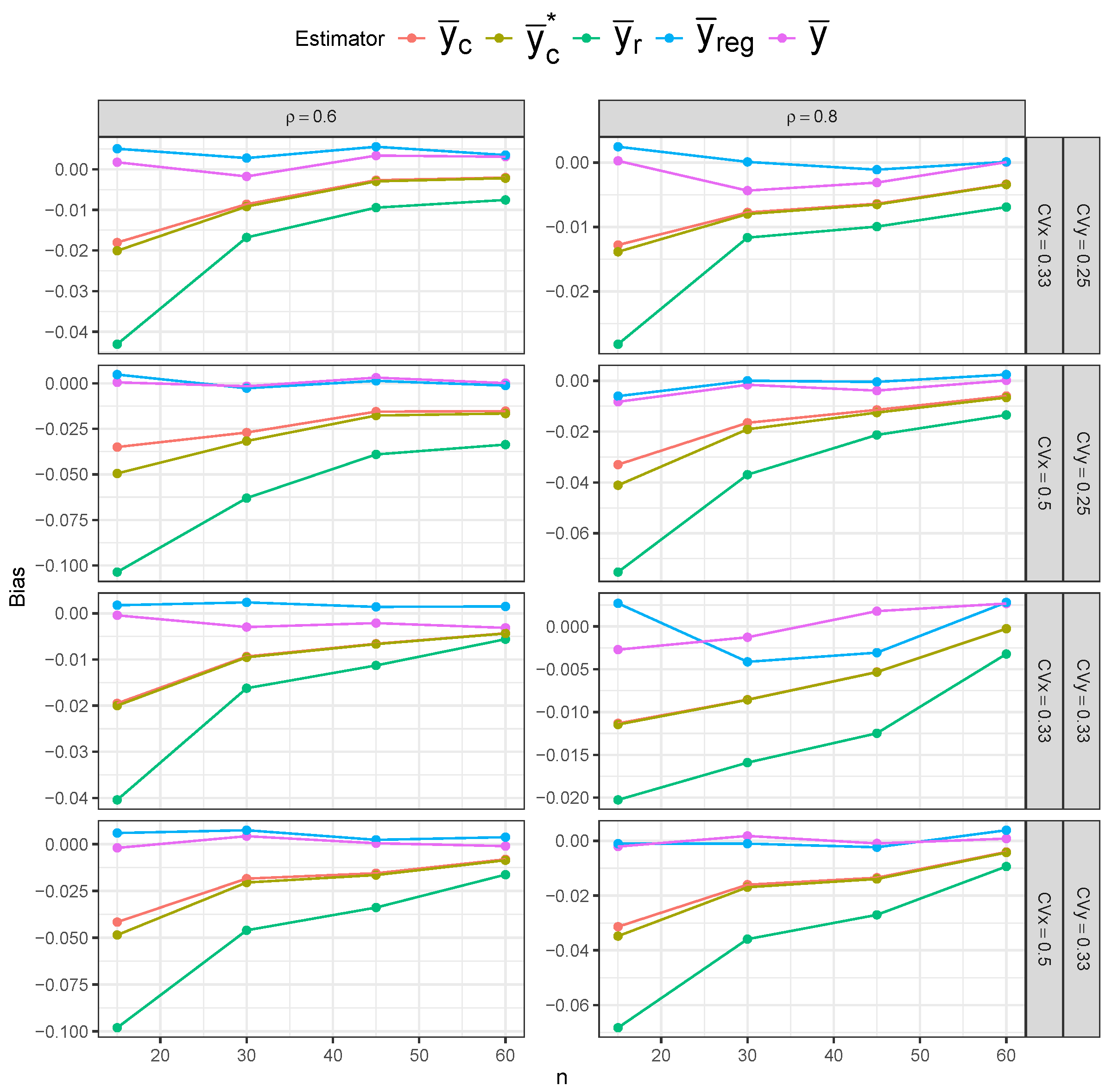
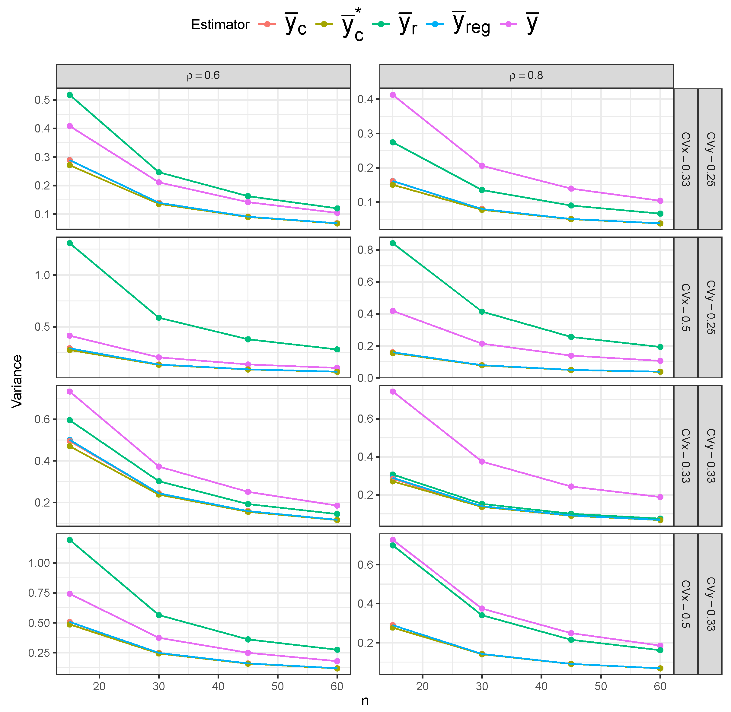
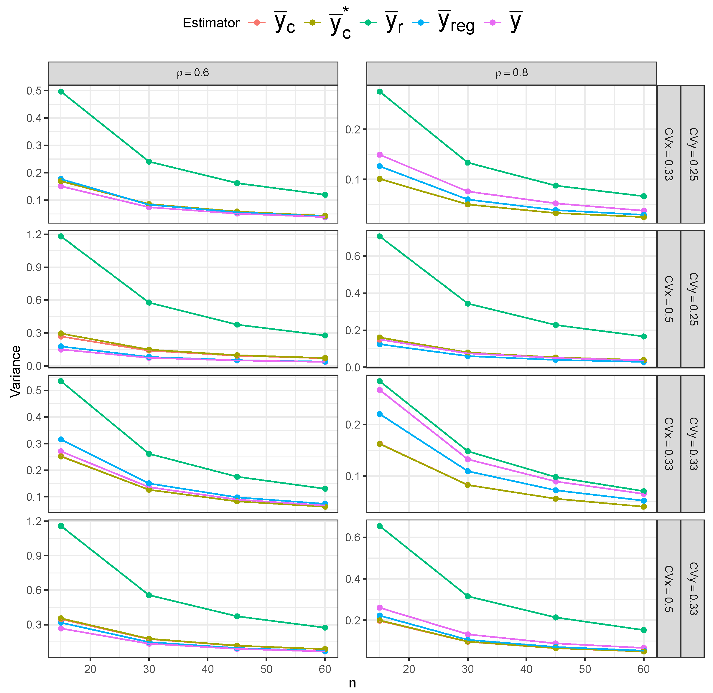
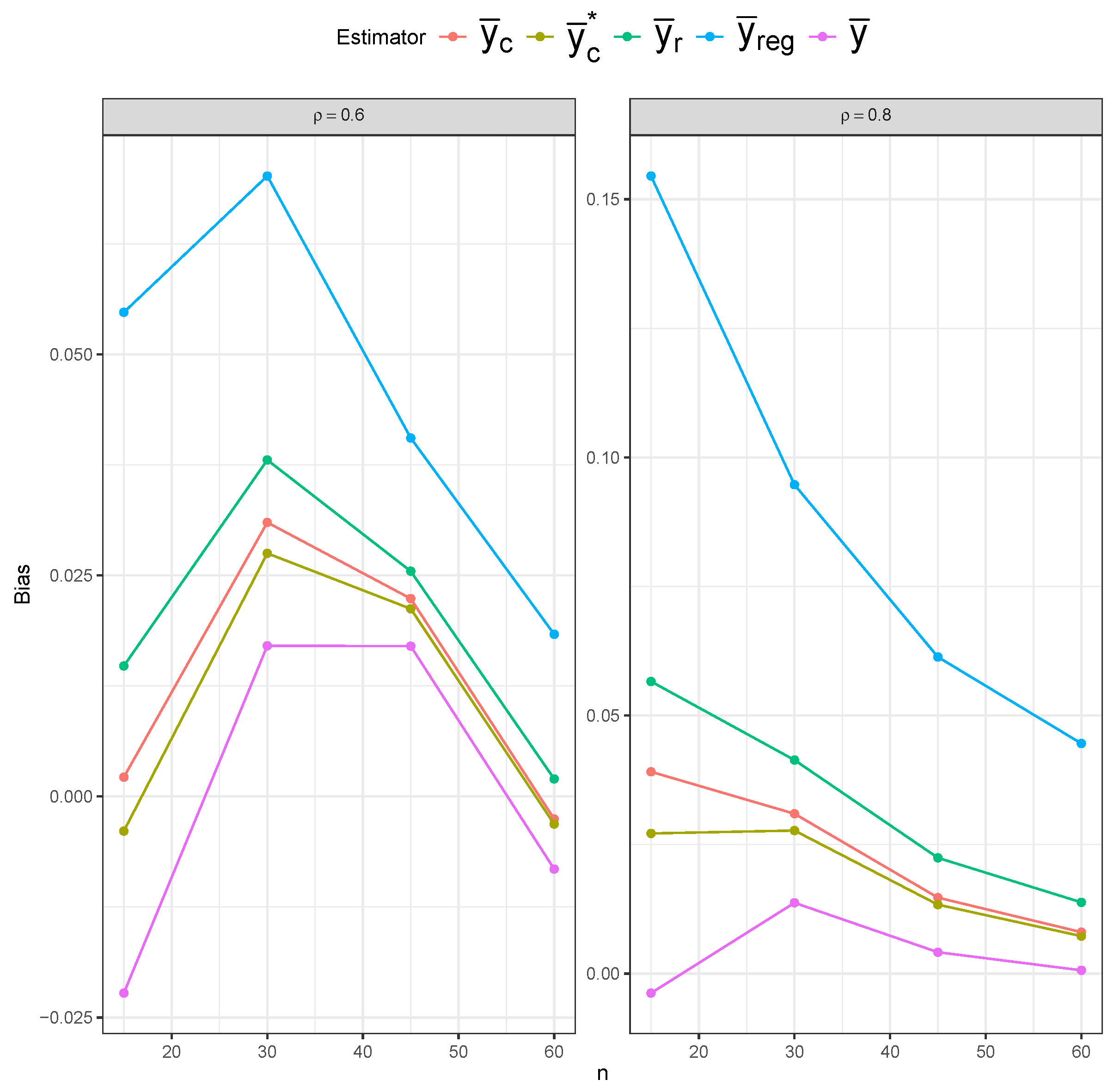
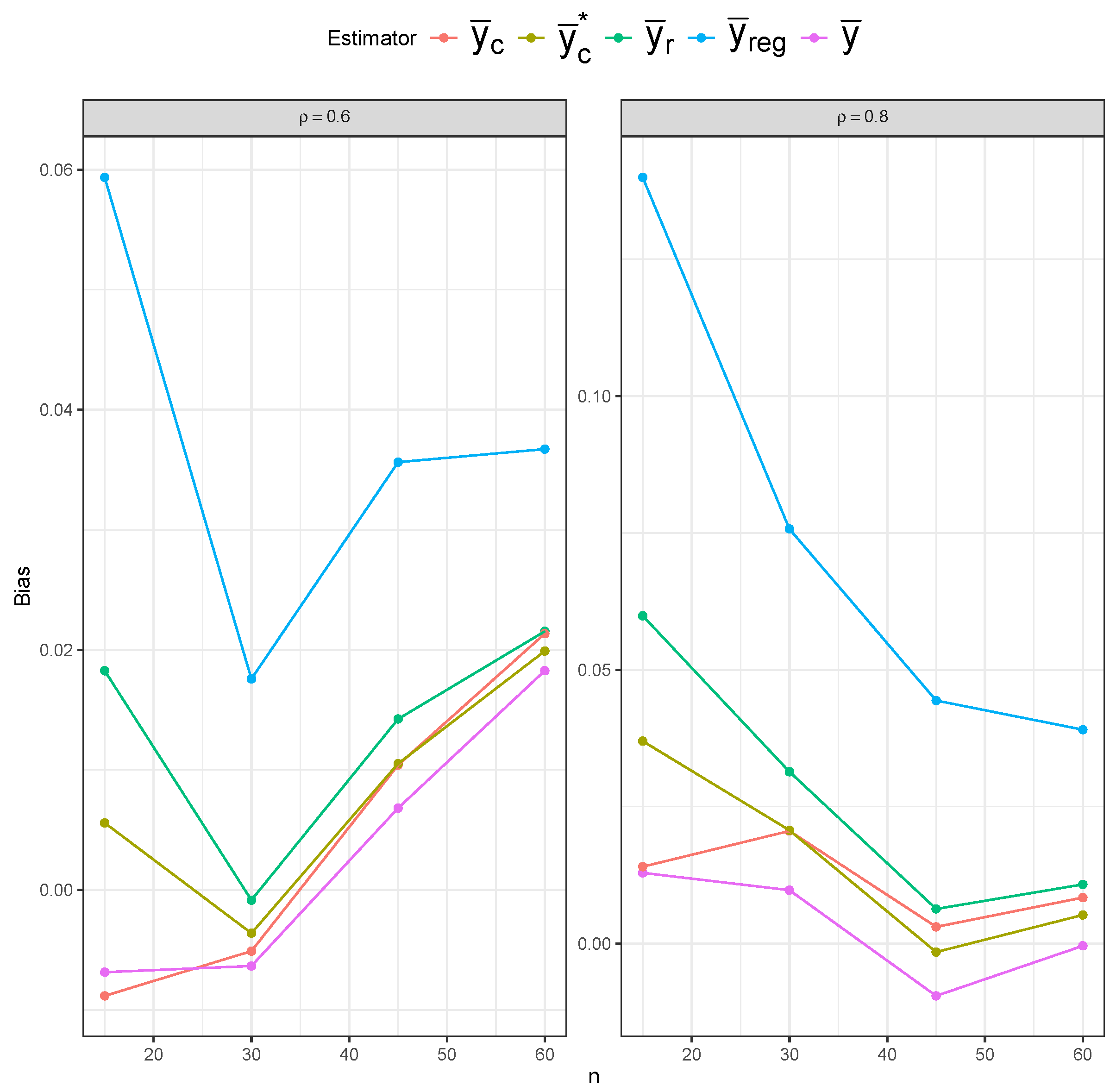
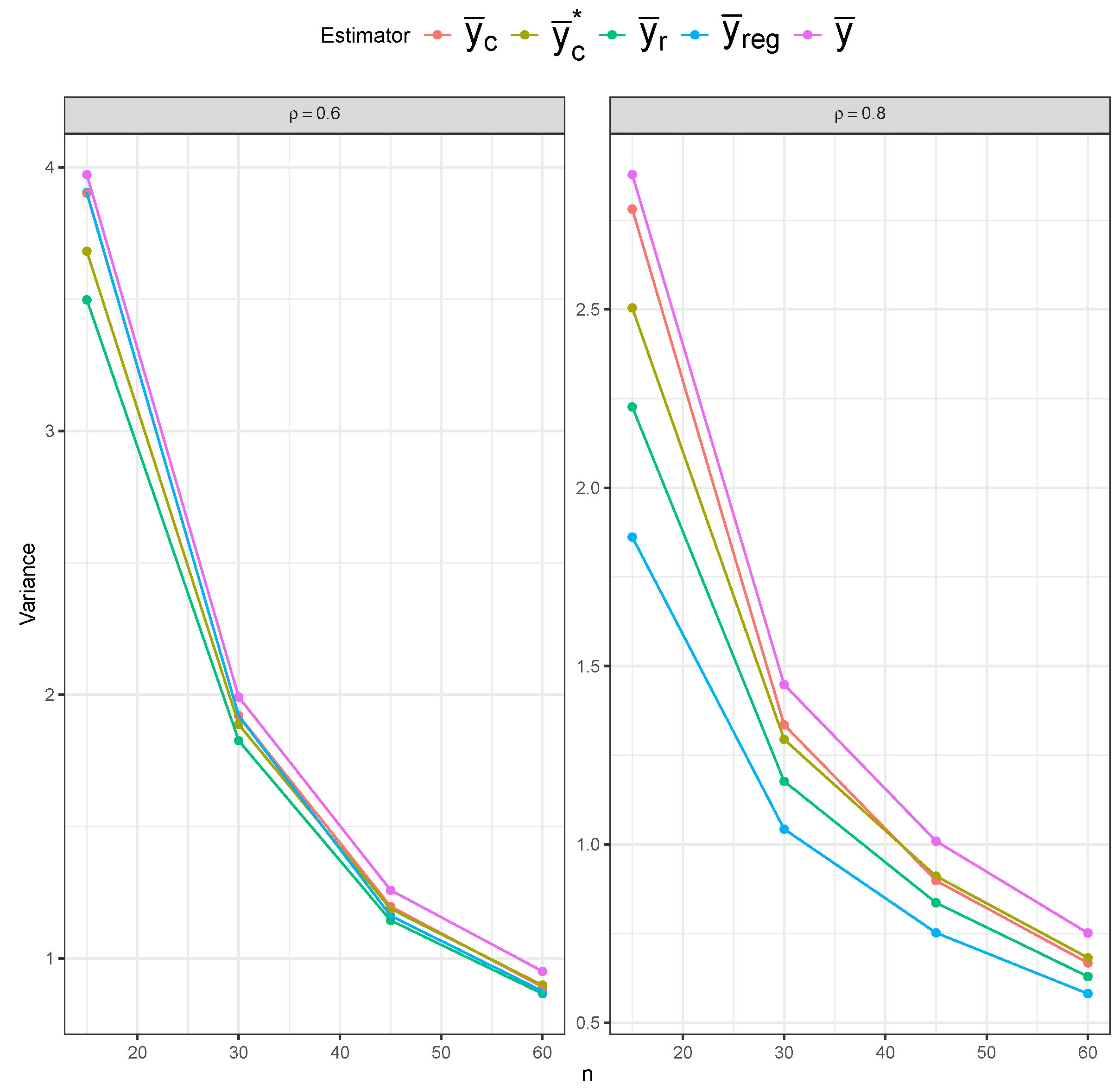
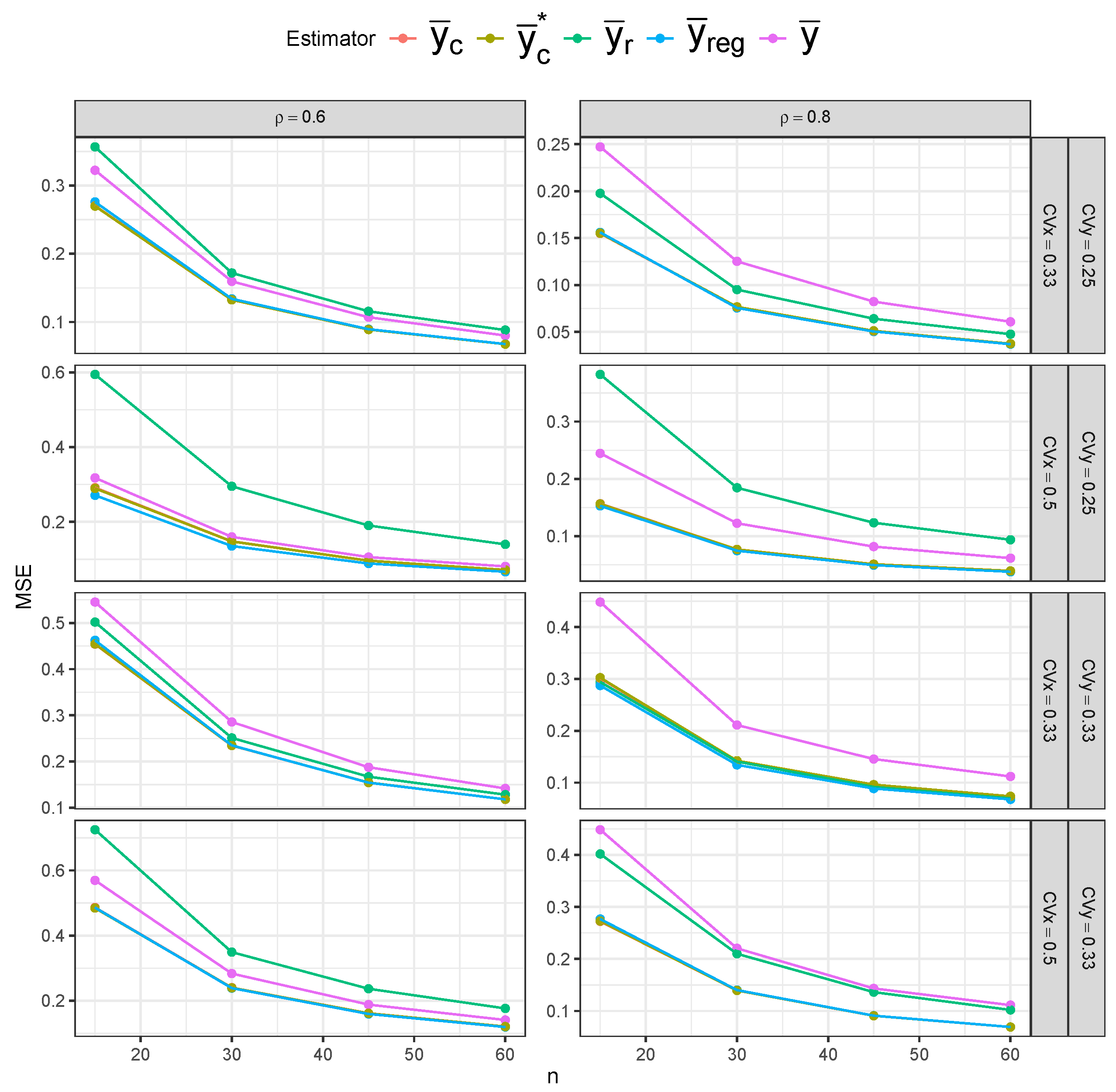
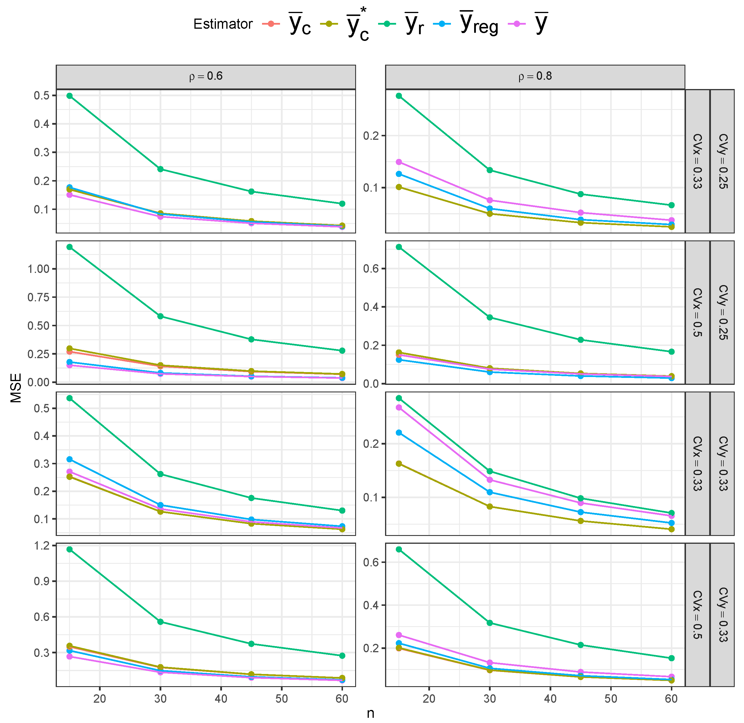
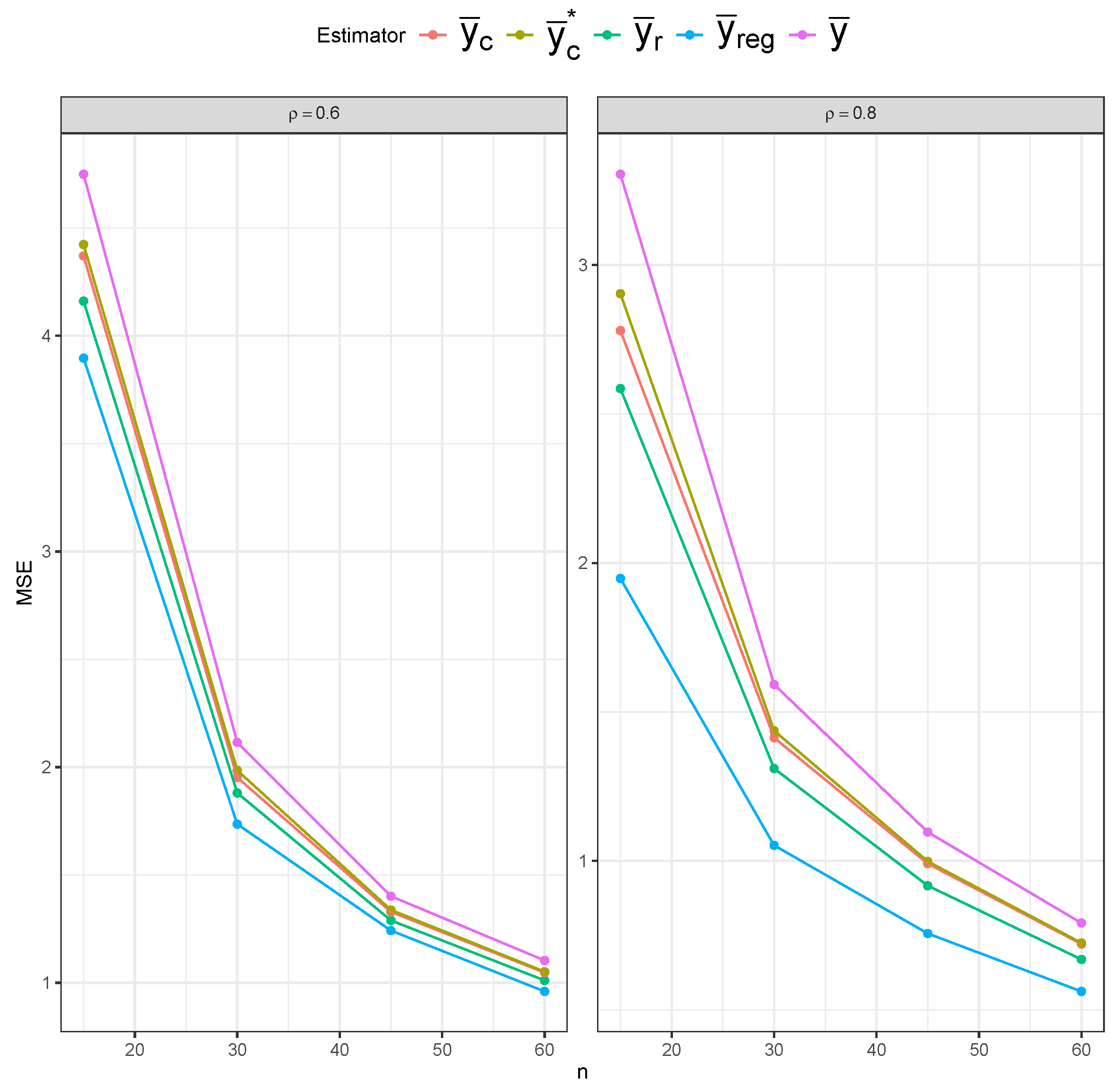
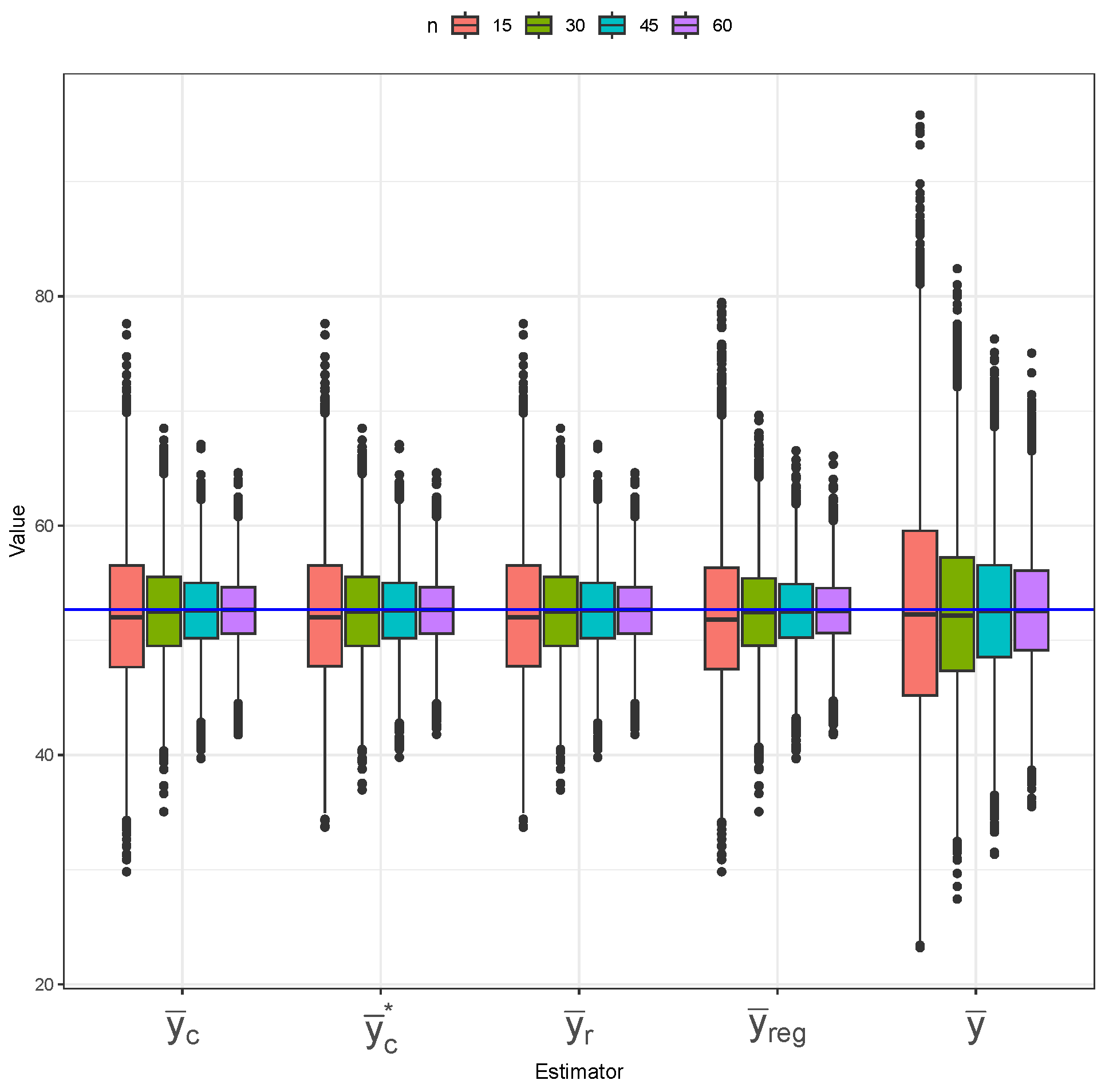
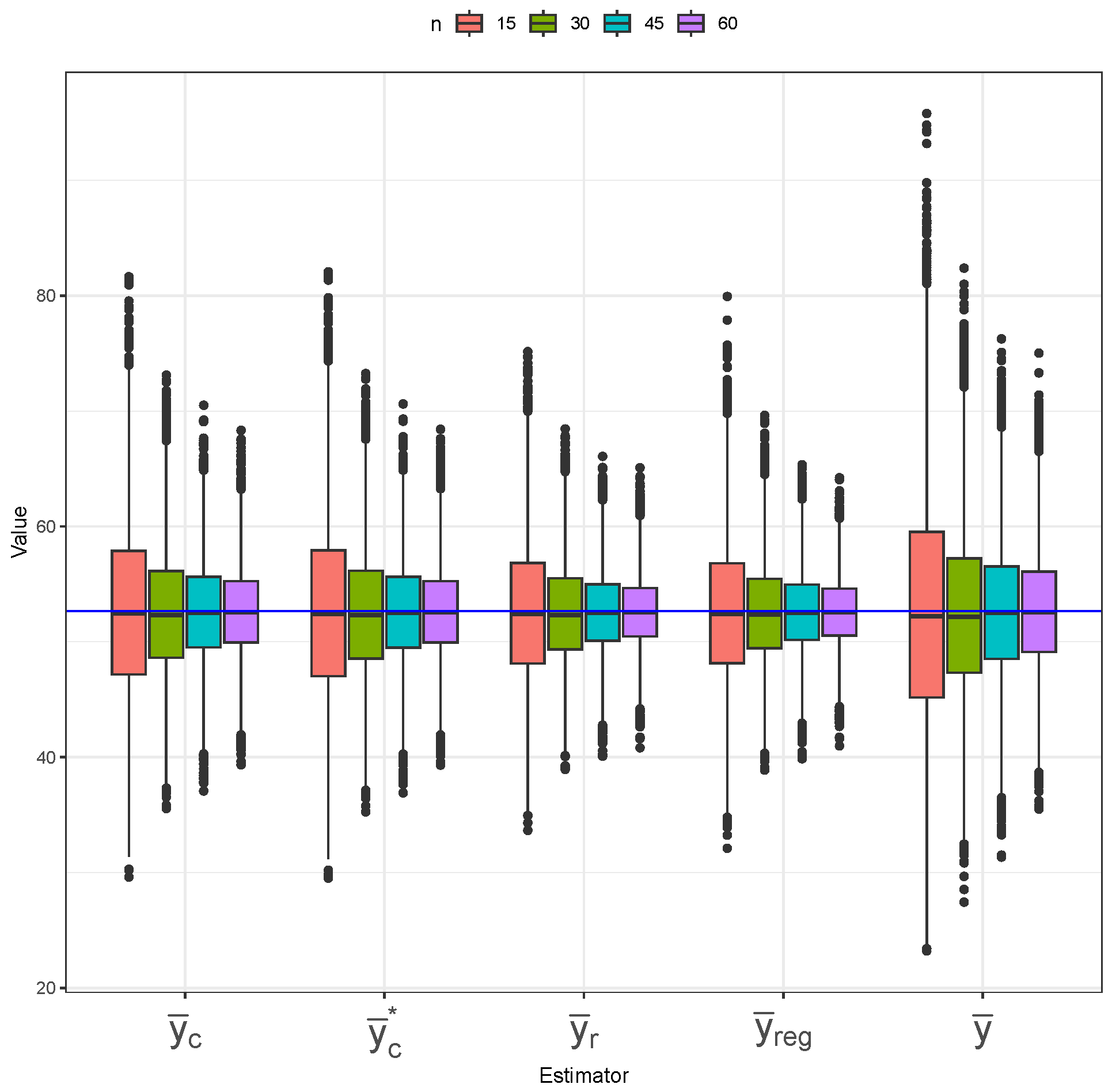
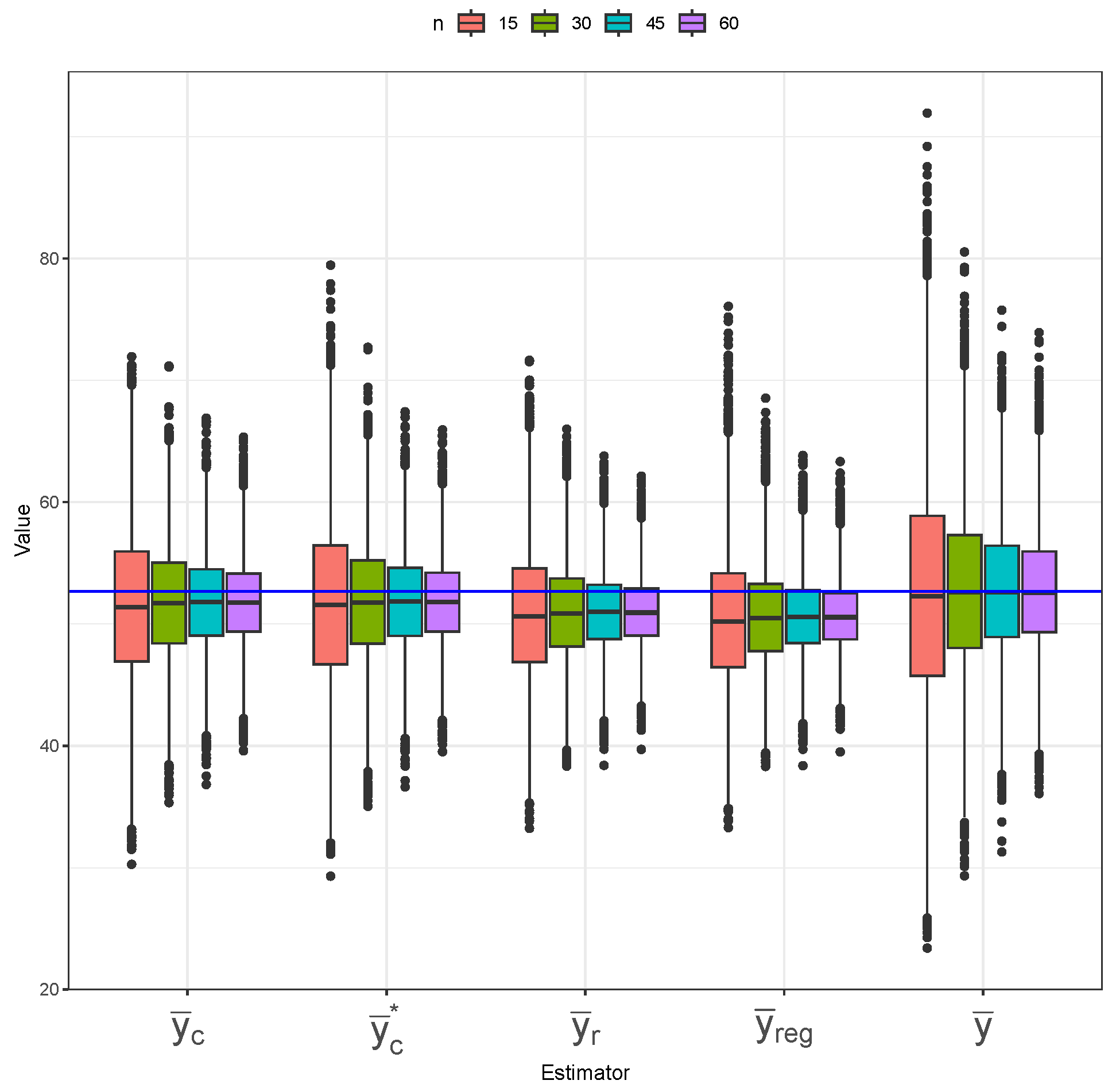
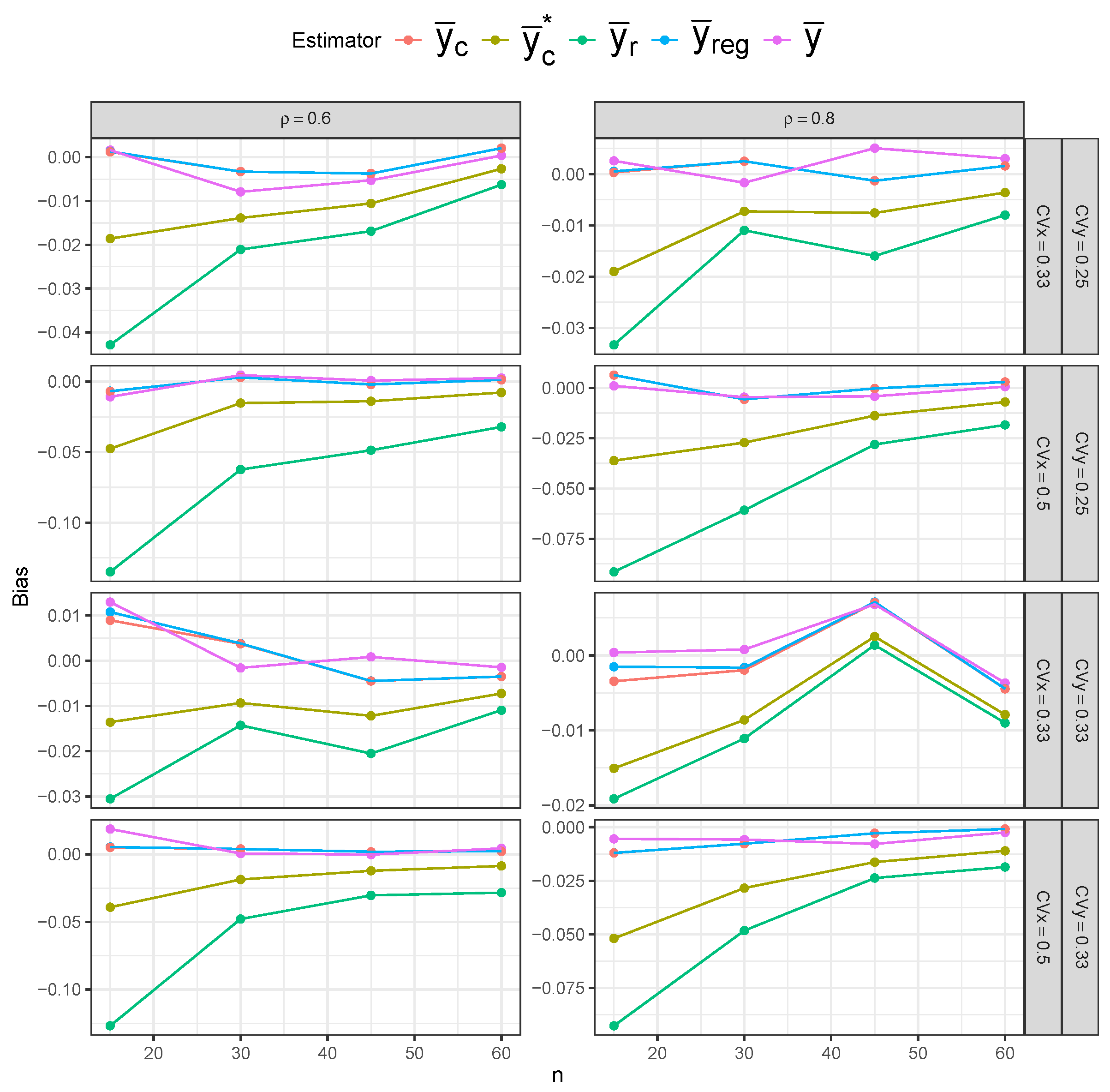
In this section, we summarize the simulation results under the normal population scenario. Figure 1, Figure 2 and Figure 3 display the Monte Carlo distribution of five estimators under SRS, imperfect-ranking RSS, and perfect-ranking RSS, respectively. The MSE results for the five estimators are presented in Figure 4, Figure 5 and Figure 6. Additional simulation results, specifically bias and variance plots, for the normal case are deferred to Appendix A.1.
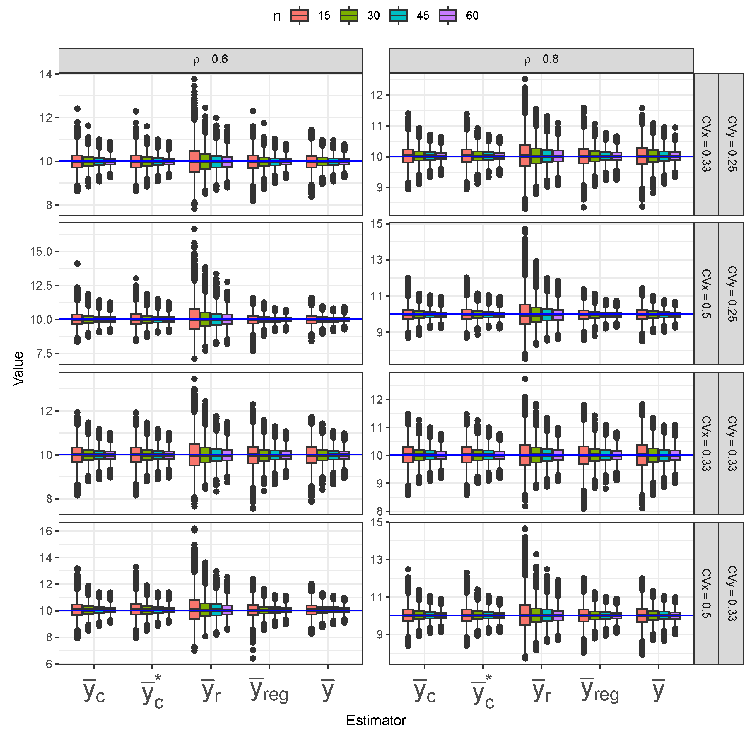
First, examining the sampling distributions of the estimators, we observe that in all three sampling designs, the ratio estimator ( y ¯ r ) consistently shows the largest interquartile range, longer whiskers, and more outliers, indicating lower efficiency and robustness, and this is especially evident under SRS; see Figure 1. On the other hand, the composite ( y ¯ c and y ¯ c * ) and regression ( y ¯ reg ) estimators show the shortest interquartile ranges and the least outliers across most scenarios, indicating relatively higher efficacy than other estimators. Although the simple mean estimator ( y ¯ ) has relatively wide interquartile ranges under SRS and imperfect-ranking RSS, it shows much-improved behavior under perfect-ranking RSS, as it benefits from improved ranking accuracy. As the sample size increases, the precision of all estimators improves, as shown by the tighter interquartile ranges. In general, all estimators demonstrate a good central tendency, as the centers of the boxplots are mostly aligned with the true mean line.
Figure 4, Figure 5 and Figure 6 illustrate the MSE performance of the five estimators under different sampling designs and parameter settings. Under all three sampling designs, the MSE decreases with increasing sample size for all estimators, supporting the consistency of these estimators. In the SRS setting (Figure 4), the simple mean ( y ¯ ) and ratio ( y ¯ r ) estimators consistently exhibit the highest MSE values across all sample sizes, indicating lower efficiency. In contrast, the composite estimators ( y ¯ c and y ¯ c * ) and the regression estimator ( y ¯ reg ) demonstrate notably lower MSE values, with the two composite estimators performing nearly identically and slightly outperforming the regression estimator. Under the imperfect-ranking RSS design (Figure 5), the simple mean and ratio estimators remain the least efficient across all conditions. The composite and regression estimators show substantial improvements in efficiency, with the two composite estimators again nearly indistinguishable and generally exhibiting the lowest MSEs. Under perfect-ranking RSS (Figure 6), the simple mean estimator shows superior relative performance for the lower-correlation setting ( ρ = 0.6 ), especially at low-to-moderate sample sizes. Under this design, the ratio estimator has the highest MSE across all parameter values. The composite estimators consistently outperform other estimators under the high-correlation setting ( ρ = 0.8 ), closely followed by the regression estimator.

4.5.2. The Lognormal Case

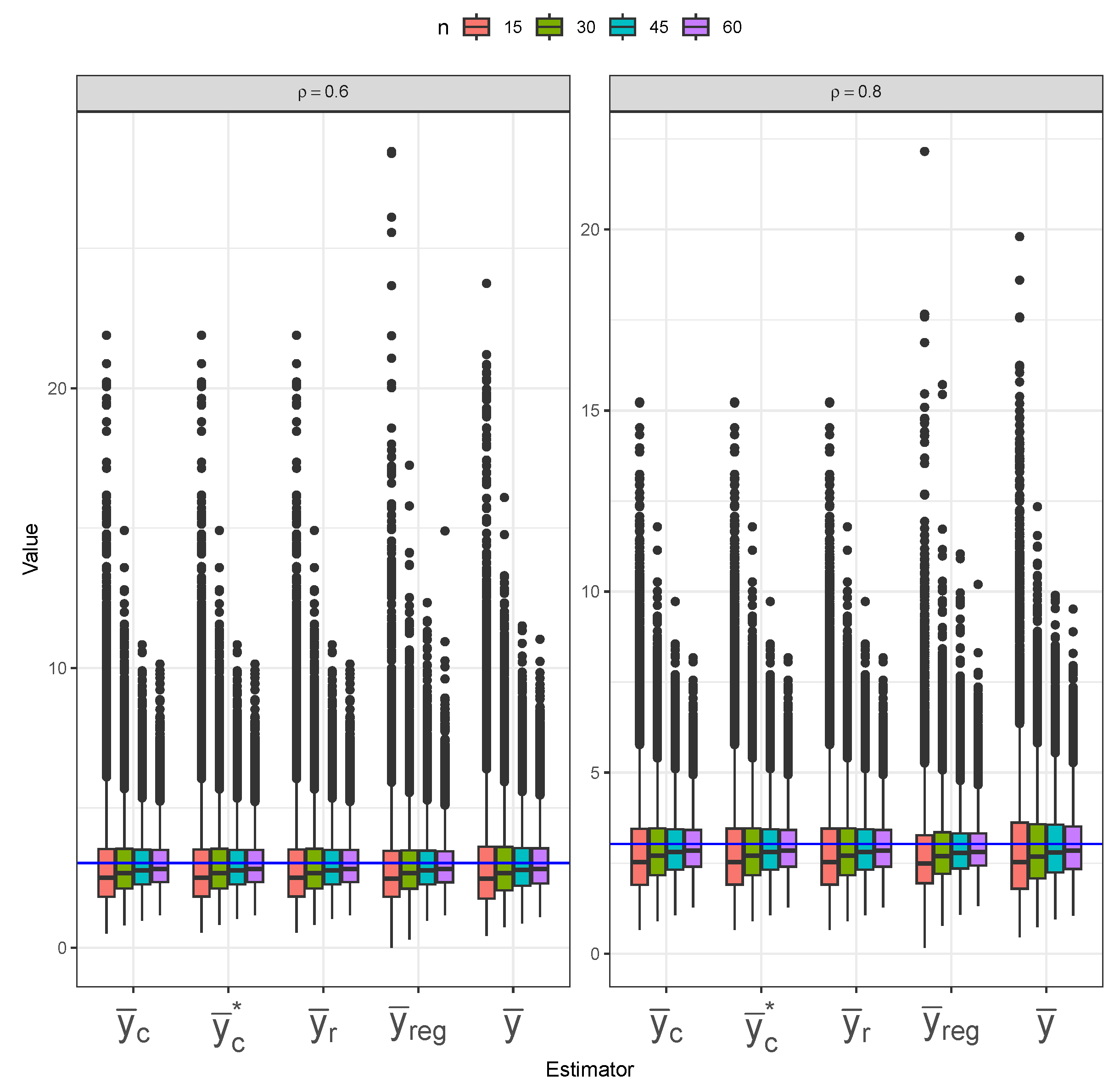
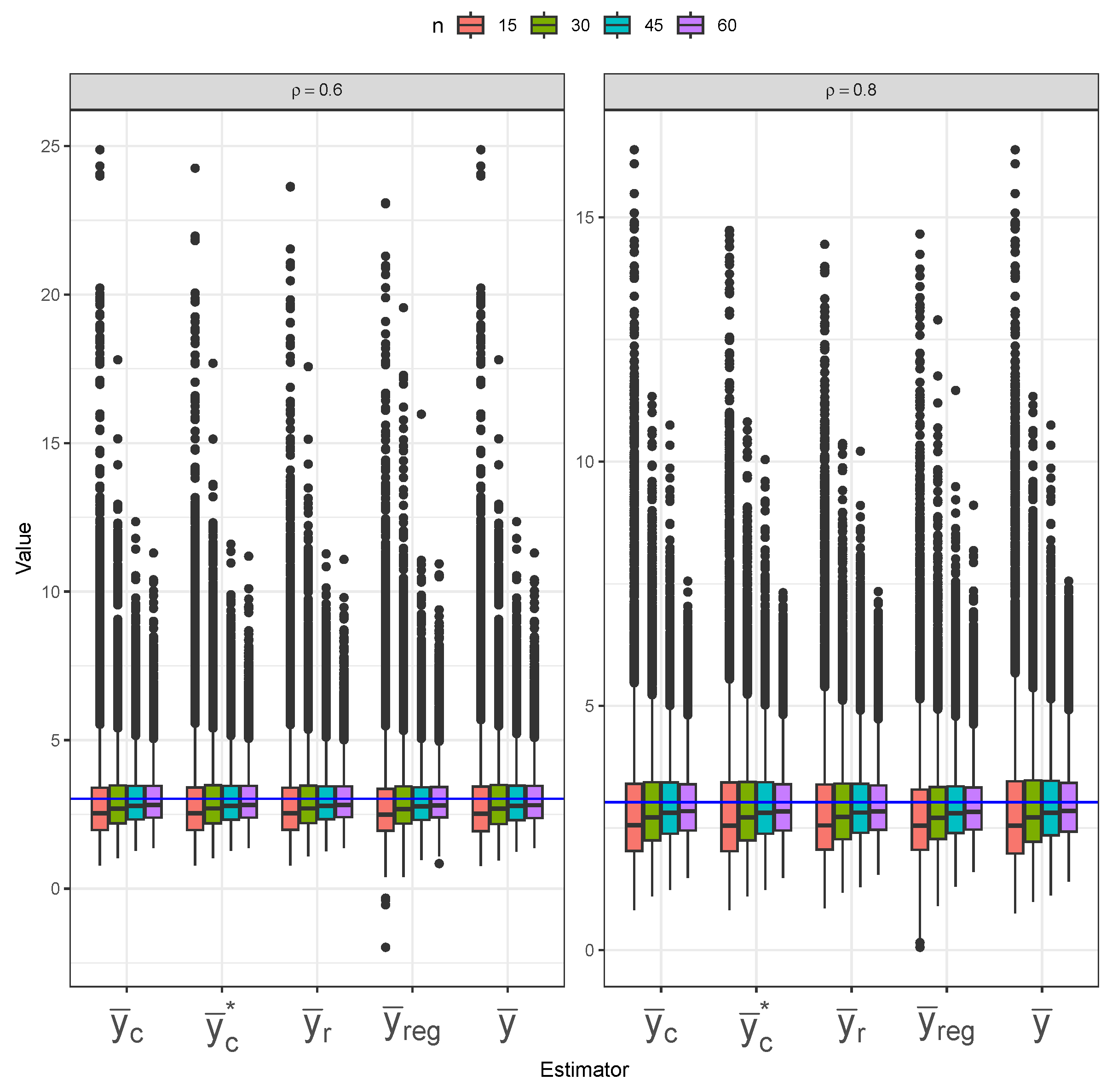
Figure 7, Figure 8 and Figure 9 present the sampling distributions of five mean estimators under lognormal populations across different sampling designs, correlation levels ( ρ = 0.6 and ρ = 0.8 ), and sample sizes ( n = 15 , 30 , 45 , 60 ). In the SRS setting (Figure 7), the composite estimators ( y ¯ c and y ¯ c * ) exhibit strong performance, with tight interquartile ranges, relatively symmetric distributions, and limited outliers. The ratio estimator ( y ¯ r ) maintains a good central tendency, but with slightly broader variability. In contrast, the regression ( y ¯ reg ) and simple mean ( y ¯ ) estimators show wider spreads and more frequent extreme values, especially for smaller sample sizes. Under the imperfect-ranking RSS design (Figure 8), all five estimators show similar behavior, with clear underestimation, as seen from the centers of all the boxplots falling below the true mean line. A similar pattern is observed under perfect-ranking RSS (Figure 9), with the regression estimator showing occasional negative outlying values and the simple mean estimator showing somewhat larger variability under the higher-correlation scenario.
Figure 10, Figure 11 and Figure 12 illustrate the MSE behavior of the five target estimators across varying sample sizes and correlation levels for lognormal populations. In the SRS setting (Figure 10), the regression ( y ¯ reg ) estimator consistently achieves the lowest MSE across all sample sizes and both correlation levels, especially under strong correlation ( ρ = 0.8 ). The composite ( y ¯ c and y ¯ c * ) and ratio ( y ¯ r ) estimators follow closely behind, showing comparable MSE performance at moderate correlation ( ρ = 0.6 ), but lagging under the stronger-correlation ( ρ = 0.8 ) scenario. The simple mean ( y ¯ ) estimator consistently has the highest MSE values. Figure 11, which corresponds to the imperfect-ranking RSS design, shows a similar overall trend, but with subtle differences. The regression estimator remains dominant, especially under ρ = 0.8 , showing the lowest MSE across all sample sizes. The ratio estimator follows in superiority, showing the second-lowest MSE values across scenarios. The composite estimators still perform well, but their advantage is less pronounced under the stronger-correlation and smaller-sample-size scenarios. The simple mean estimator again show relatively higher MSE values, remaining the least efficient. Under perfect ranking (Figure 12), while all estimators have similar MSE curves, the ratio estimator, followed by the composite estimator ( y ¯ c * ), achieves the lowest MSE values at ρ = 0.6 . When ρ = 0.8 , the pattern closely replicates that observed under imperfect-ranking RSS.
Across all figures, the MSE decreases with increasing sample size for all estimators, reflecting improved estimation precision. These results highlight that while the regression estimator offers the best performance overall—particularly in the high-correlation setting—composite and ratio estimators provide competitive alternatives, especially as the ranking accuracy improves.
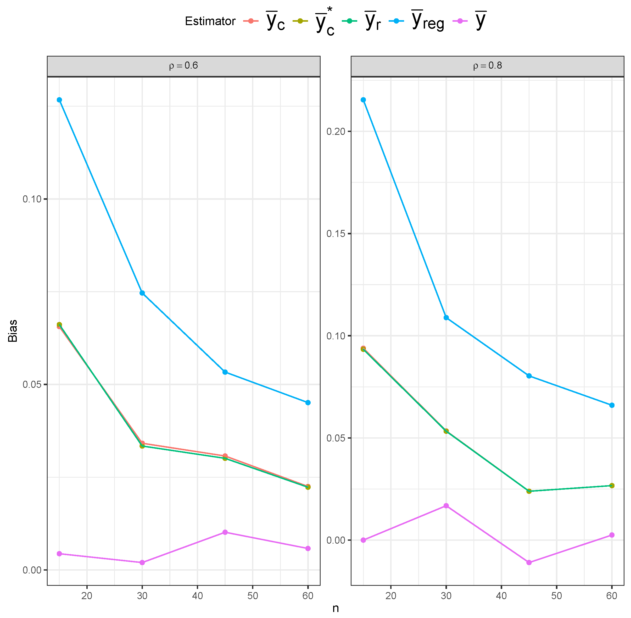
Additional simulation results, including bias and variance graphs under lognormal data, are located in Appendix A.2.

5. Real Data Application

For the real data application, we use a modified version of the longleaf pine dataset comprising N = 396 trees, as analyzed by Jafari Jozani and Johnson [20]. The original dataset can be found in Chen et al. [21] and Platt et al. [22]. In this dataset, the variable X denotes tree diameter at breast height, while Y represents tree height [20]. To remove ties when ranking based on the X variable, a small amount of random noise was added to the X variable: ε x N ( 0 , 0.000001 ) , recentered at zero. The Pearson correlation between the transformed X variable and the Y variable was ρ = 0.91 . Considering the N = 396 observations as the finite population, we drew 10,000 samples using each of three sampling designs—SRS, RSS with imperfect ranking (ranking based on X), and RSS with perfect ranking (ranking based on Y)—and computed each of the five estimators considered in the simulation study in the previous section. Goodness-of-fit tests—using the Shapiro—Wilk (‘sw’) option in the ‘gofTest()’ function of the EnvStats package ver. 3.1.0 in R [23]—confirmed that both X and Y can be modeled by the lognormal distribution, justifying the application of the lognormal approximation of the moments of sample order statistics (see Equation (23)) under this dataset.
Figure 13, Figure 14 and Figure 15 present the distribution of five mean estimators under different sampling designs applied to the longleaf pine dataset, with the blue horizontal line indicating the true population mean. In Figure 13 (SRS), the simple mean estimator ( y ¯ ) exhibits the greatest variance, as its boxplots are widely spread. The ratio ( y ¯ r ) and composite ( y ¯ c and y ¯ c * ) estimators perform best under SRS, showing less outliers and relatively low variance. The regression ( y ¯ reg ) estimator follows with slightly higher outlier presence, especially at small sample sizes. All estimators show low-to-no bias, as the boxplots are mostly centered at the true population mean. Similar patterns are observed under imperfect-ranking RSS (Figure 14), but with the composite estimators switching places with the regression estimators. Under perfect-ranking RSS (Figure 15), the simple mean estimator still shows the largest variability across different sample sizes, but it possesses the least bias overall. The ratio and regression estimators again show slightly lower variability than the composite estimators. However, the composite estimators are more centered around the true mean, indicating lower bias than the ratio and regression estimators.
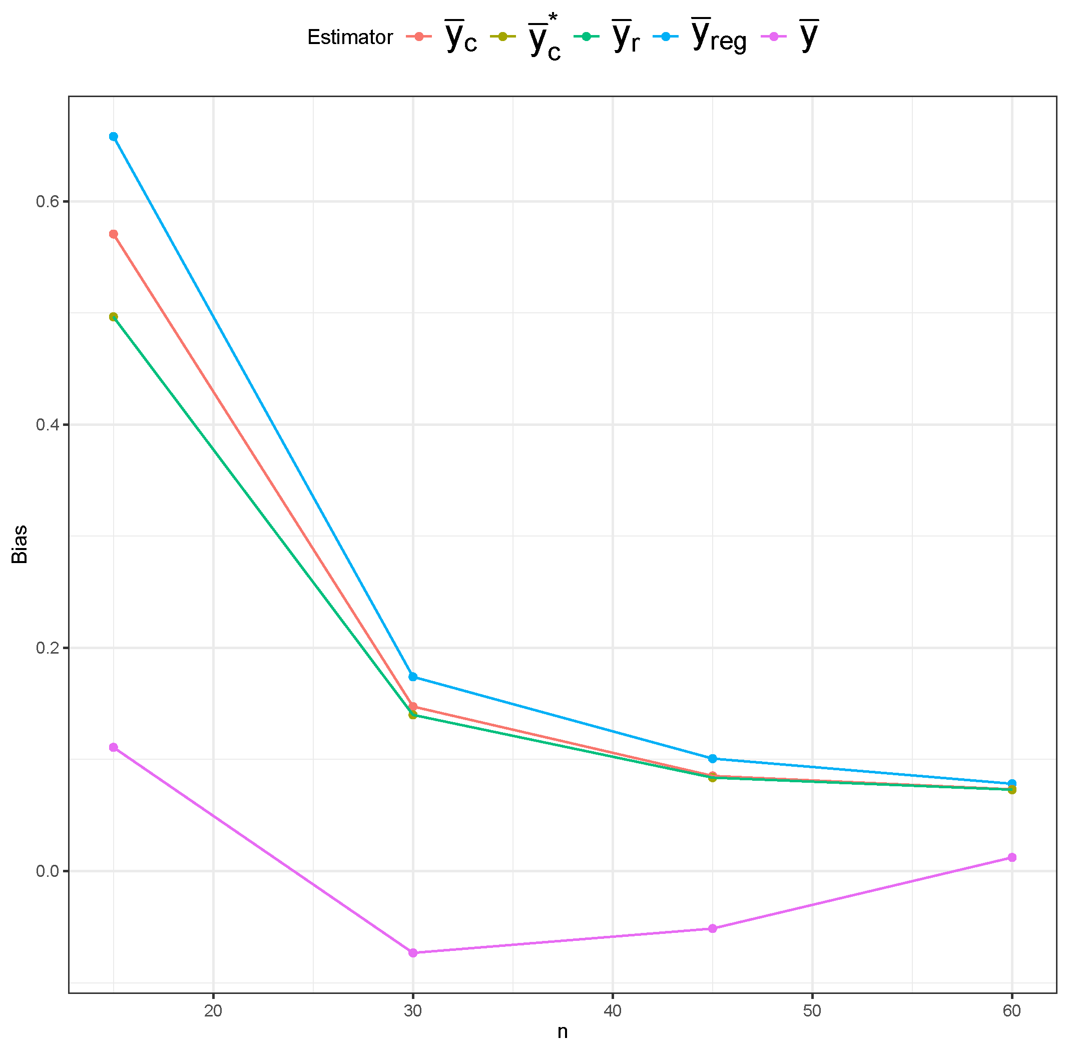
Table 1 displays the MSE behavior of five estimators under the SRS and RSS designs. The bias and variance results are included in Appendix A.3. Across all three sampling designs, the simple mean estimator ( y ¯ ) exhibits notably higher MSE values than the other estimators across all sample sizes, confirming its inefficiency. However, the impact of the sampling design on the simple mean estimator’s MSE is most evident, as we can clearly see lower MSE values under RSS than under SRS, and under perfect-ranking RSS than under imperfect-ranking RSS. The remaining four estimators have similar MSE values under SRS. The ratio ( y ¯ r ) and regression ( y ¯ reg ) estimators show superior performance under imperfect-ranking RSS across all sample sizes. The superiority of the ratio and regression estimators remains under perfect-ranking RSS, especially for the smaller sample sizes, with the composite estimators ( y ¯ c and y ¯ c * ) approaching them for the larger sample sizes ( n = 45 , 60 ).

6. Discussion

In this study, we introduced a composite estimator for estimating the finite population mean under RSS. The estimator is defined as a weighted average of the simple mean and the ratio estimator. We derived its MSE and obtained the optimal weight that minimizes the MSE, along with a plug-in estimator for this optimal weight. We evaluated the performance of the composite estimator—both with the known optimal weight and the estimated (plug-in) weight—via Monte Carlo simulations using bivariate normal and lognormal populations, as well as a real finite population of longleaf pine trees. Comparisons were made against the simple mean, ratio, and regression estimators under SRS, imperfect-ranking RSS, and perfect-ranking RSS. The results indicate that the proposed composite estimator is highly efficient, particularly for moderate-to-large sample sizes, even in cases where the simple mean and ratio estimators perform poorly. The regression estimator consistently emerged as a strong competitor across all settings. For all three designs, the performance of the composite, ratio, and regression estimators improved as the correlation between the study and auxiliary variables increased. This trend also benefited the simple mean estimator under imperfect-ranking RSS, as higher correlation improved ranking accuracy. These findings were consistent across normal, lognormal, and real data scenarios. Although the plug-in version of the composite estimator performed well, its efficiency may be further enhanced through refinements in estimating the optimal weight. A key step in this process involves estimating the moments of the order statistics, μ x ( k ) and μ y [ k ] , which we approximated using known formulas for normal and lognormal distributions. Similar approximations exist for other distributions and could be explored in future work. Another promising direction is extending composite estimators to settings with multivariate auxiliary variables, where one or more variables could be used for ranking, estimation, or both. Such generalizations could further enhance the utility and flexibility of composite estimators for survey data.
Author Contributions

Conceptualization, S.A.M. and S.J.; methodology, S.A.M. and S.J.; software, S.A.M., T.J.III, and S.J.; formal analysis, S.A.M. and S.J.; investigation, S.A.M., T.J.III, and S.J.; resources, S.A.M.; data curation, T.J.III; writing—original draft preparation, T.J.III and S.J.; writing—review and editing, S.A.M., T.J.III, and S.J.; supervision, S.A.M.; project administration, S.A.M. All authors have read and agreed to the published version of the manuscript.

Funding

This work of Thomas Johnson III was funded by the North Carolina A&T State University Chancellor’s Distinguished Fellowship, a Title III HBGI grant from the U.S. Department of Education.

Data Availability Statement

The original data presented in the study are openly available in [5].

Conflicts of Interest

The authors declare no conflicts of interest.

Appendix A. Additional Simulation Results

Appendix A.1. The Normal Case

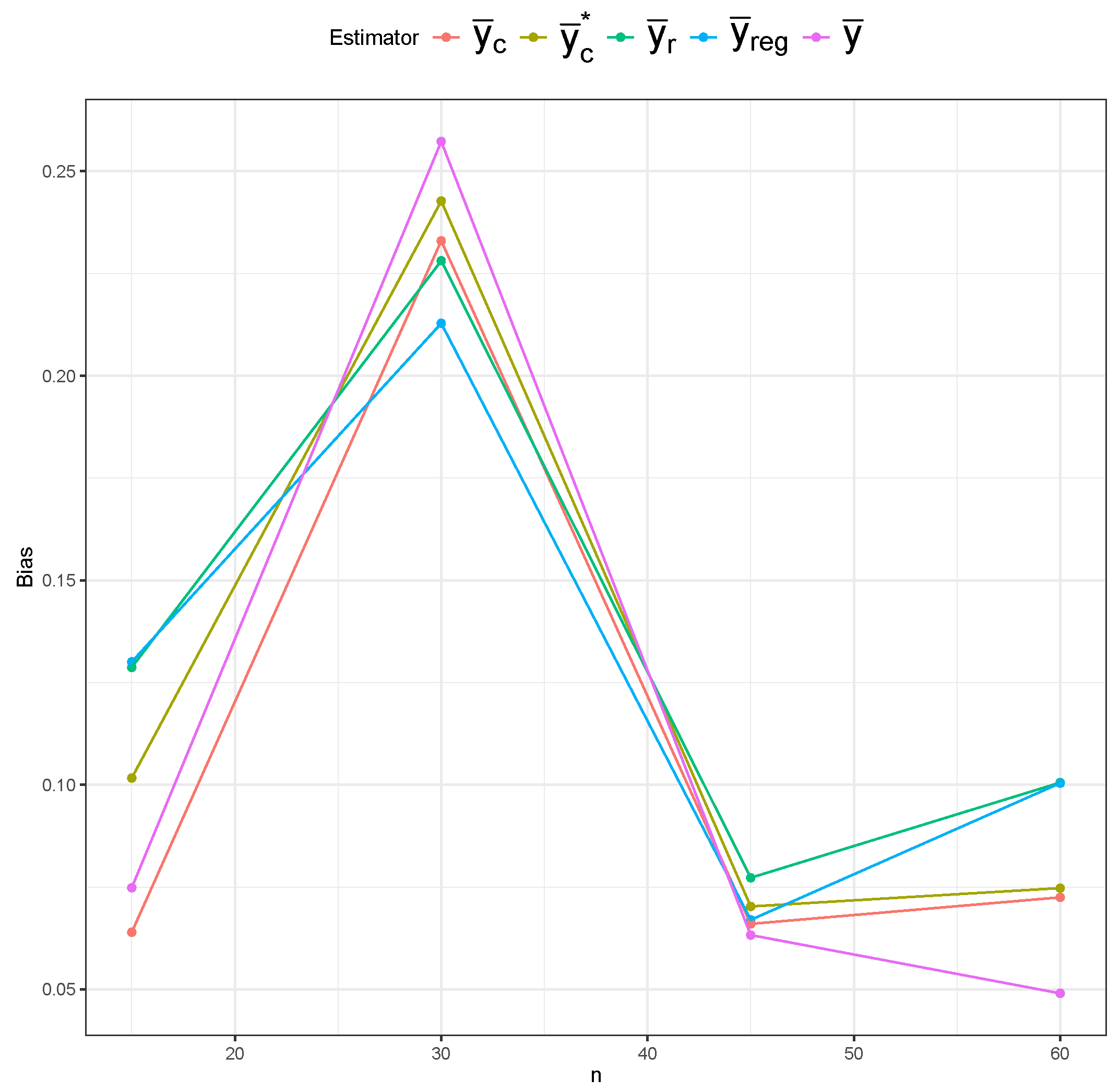
Figure A1. Bias of five mean estimators under SRS from normal population.
Mathematics 13 03071 g0a1
Figure A2. Bias of five mean estimators under imperfect-ranking RSS (fixing p = 5 ) from normal population.
Mathematics 13 03071 g0a2
Figure A3. Bias of five mean estimators under perfect-ranking RSS (fixing p = 5 ) from normal population.
Mathematics 13 03071 g0a3
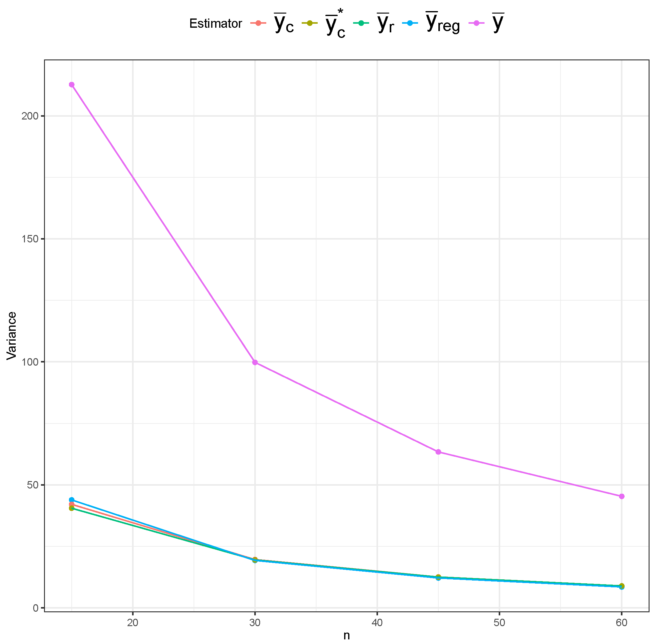
Figure A4. Variance of five mean estimators under SRS from normal population.
Mathematics 13 03071 g0a4
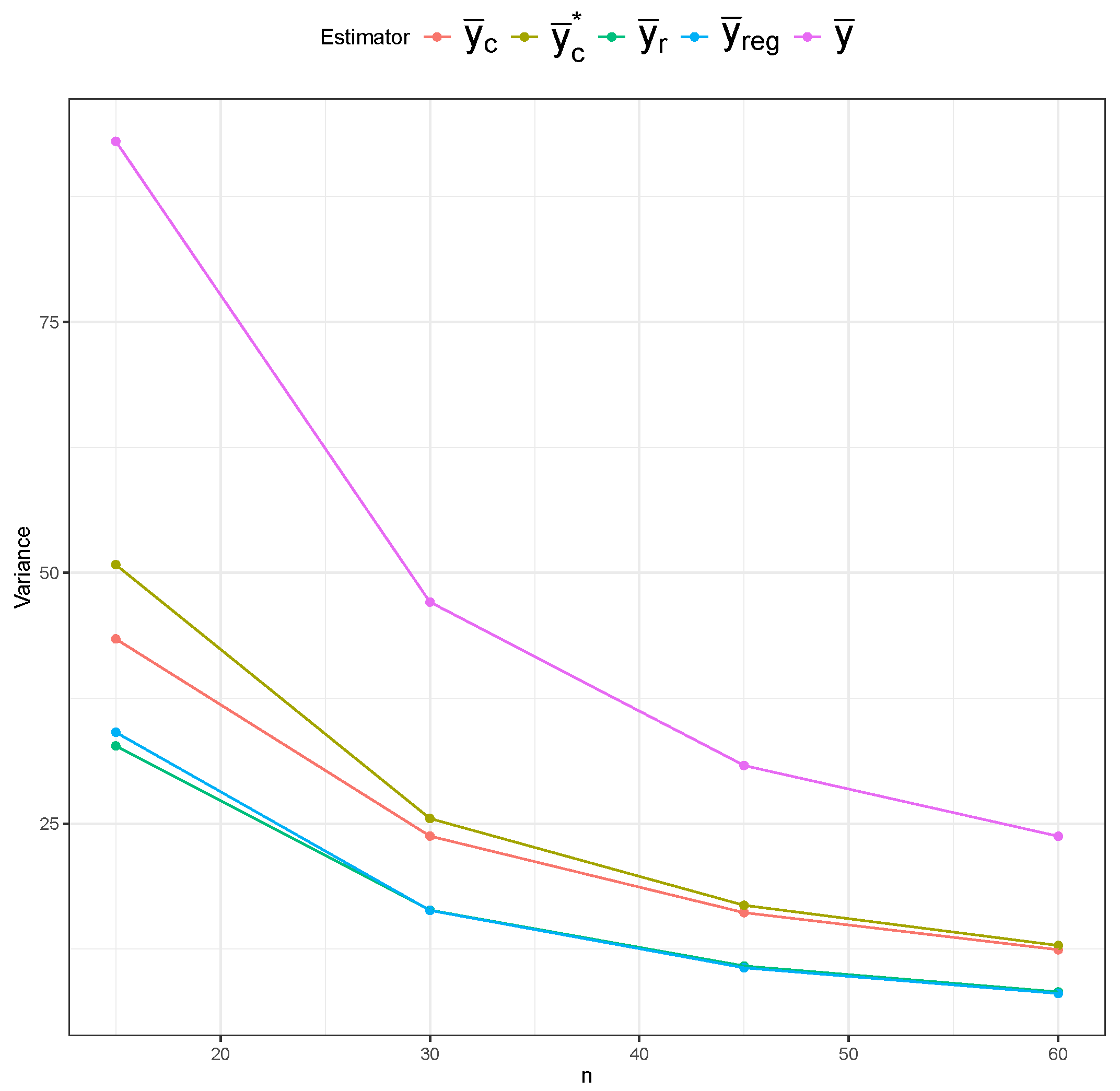
Figure A5. Variance of five mean estimators under imperfect-ranking RSS (fixing p = 5 ) from normal population.
Mathematics 13 03071 g0a5
Figure A6. Variance of five mean estimators under perfect-ranking RSS (fixing p = 5 ) from normal population.
Mathematics 13 03071 g0a6

Appendix A.2. The Lognormal Case

Figure A7. Bias of five mean estimators under SRS from lognormal population.
Mathematics 13 03071 g0a7
Figure A8. Bias of five mean estimators under imperfect-ranking RSS (fixing p = 5 ) from lognormal population.
Mathematics 13 03071 g0a8
Figure A9. Bias of five mean estimators under perfect-ranking RSS (fixing p = 5 ) from lognormal population.
Mathematics 13 03071 g0a9
Figure A10. Variance of five mean estimators under SRS from lognormal population.
Mathematics 13 03071 g0a10
Figure A11. Variance of five mean estimators under imperfect-ranking RSS (fixing p = 5 ) from lognormal population.
Mathematics 13 03071 g0a11
Figure A12. Variance of five mean estimators under perfect-ranking RSS (fixing p = 5 ) from lognormal population.
Mathematics 13 03071 g0a12

Appendix A.3. Real Data Application

Figure A13. Bias of five mean estimators under SRS from longleaf pine dataset.
Mathematics 13 03071 g0a13
Figure A14. Bias of five mean estimators under imperfect-ranking RSS (fixing p = 5 ) from longleaf pine dataset.
Mathematics 13 03071 g0a14
Figure A15. Bias of five mean estimators under perfect-ranking RSS (fixing p = 5 ) from longleaf pine dataset.
Mathematics 13 03071 g0a15
Figure A16. Variance of five mean estimators under SRS from longleaf pine dataset.
Mathematics 13 03071 g0a16
Figure A17. Variance of five mean estimators under imperfect-ranking RSS (fixing p = 5 ) from longleaf pine dataset.
Mathematics 13 03071 g0a17
Figure A18. Variance of five mean estimators under perfect-ranking RSS (fixing p = 5 ) from longleaf pine dataset.
Mathematics 13 03071 g0a18

References

  1. McIntyre, G.A. A method for unbiased selective sampling using ranked sets. Aust. J. Agric. Res. 1952, 3, 385–390. [Google Scholar] [CrossRef]
  2. Wolfe, D.A. Ranked set sampling: An approach to more efficient data collection. Stat. Sci. 2004, 19, 636–643. [Google Scholar] [CrossRef]
  3. Takahasi, K.; Wakimoto, K. On unbiased estimates of the population mean based on the sample stratified by means of ordering. Ann. Inst. Stat. Math. 1968, 20, 1–31. [Google Scholar] [CrossRef]
  4. Stokes, S.L. Estimation of Variance Using Judgment Ordered Ranked Set Samples. Biometrics 1980, 36, 35–42. [Google Scholar] [CrossRef]
  5. Chen, Z. On ranked-set sample quantiles and their applications. J. Stat. Plan. Inference 2000, 83, 125–135. [Google Scholar] [CrossRef]
  6. Stokes, S.L.; Sager, T.W. Characterization of a Ranked-Set Sample with Application to Estimating Distribution Functions. J. Am. Stat. Assoc. 1988, 83, 374–381. [Google Scholar] [CrossRef]
  7. Bohn, L.L.; Wolfe, D.A. Nonparametric Two-Sample Procedures for Ranked-Set Samples Data. J. Am. Stat. Assoc. 1992, 87, 552–561. [Google Scholar] [CrossRef]
  8. Hettmansperger, T.P. The ranked-set sample sign test. J. Nonparametric Stat. 1995, 4, 263–270. [Google Scholar] [CrossRef]
  9. Koti, K.M.; Jogesh Babu, G. Sign test for ranked-set sampling. Commun. Stat.-Theory Methods 1996, 25, 1617–1630. [Google Scholar] [CrossRef]
  10. Chen, Z. Density estimation using ranked-set sampling data. Environ. Ecol. Stat. 1999, 6, 135–146. [Google Scholar] [CrossRef]
  11. Wolfe, D.A. Ranked set sampling. Wiley Interdiscip. Rev. Comput. Stat. 2010, 2, 460–466. [Google Scholar] [CrossRef]
  12. Cochran, W.G. Sampling Techniques, 3rd ed.; Wiley: New York, NY, USA, 1977. [Google Scholar] [CrossRef]
  13. Samawi, H.M.; Muttlak, H.A. Estimation of ratio using rank set sampling. Biom. J. 1996, 38, 753–764. [Google Scholar] [CrossRef]
  14. Kadilar, C.; Unyazici, Y.; Cingi, H. Ratio estimator for the population mean using ranked set sampling. Stat. Pap. 2009, 50, 301–309. [Google Scholar] [CrossRef]
  15. Philip, L.; Lam, K. Regression estimator in ranked set sampling. Biometrics 1997, 53, 1070–1080. [Google Scholar] [CrossRef]
  16. Lui, K.J. Notes on Use of the Composite Estimator: An Improvement of the Ratio Estimator. J. Off. Stat. 2020, 36, 137–149. [Google Scholar] [CrossRef]
  17. Sevinc, B.; Cetintav, B.; Esemen, M.; Gurler, S. RSSampling: Ranked Set Sampling, R package version 1.0; 2018. Available online: https://CRAN.R-project.org/package=RSSampling (accessed on 21 July 2025).
  18. Royston, J.P. Algorithm AS 177: Expected Normal Order Statistics (Exact and Approximate). J. R. Stat. Society. Ser. C (Appl. Stat.) 1982, 31, 161–165. [Google Scholar] [CrossRef]
  19. Nadarajah, S. Explicit expressions for moments of log normal order statistics. Econ. Qual. Control 2008, 23, 267–279. [Google Scholar] [CrossRef]
  20. Jafari Jozani, M.; Johnson, B.C. Design based estimation for ranked set sampling in finite populations. Environ. Ecol. Stat. 2011, 18, 663–685. [Google Scholar] [CrossRef]
  21. Chen, Z.; Bai, Z.; Sinha, B.K. Ranked Set Sampling: Theory and Applications; Springer: Berlin/Heidelberg, Germany, 2004; Volume 176. [Google Scholar] [CrossRef]
  22. Platt, W.J.; Evans, G.W.; Rathbun, S.L. The population dynamics of a long-lived conifer (Pinus palustris). Am. Nat. 1988, 131, 491–525. [Google Scholar] [CrossRef]
  23. Millard, S.P. EnvStats: An R Package for Environmental Statistics; Springer: New York, NY, USA, 2013. [Google Scholar] [CrossRef]
Figure 1. Distribution of five mean estimators under SRS from normal population.
Mathematics 13 03071 g001
Figure 2. Distribution of five mean estimators under imperfect-ranking RSS (fixing p = 5 ) from normal population.
Mathematics 13 03071 g002
Figure 3. Distribution of five mean estimators under perfect-ranking RSS (fixing p = 5 ) from normal population.
Mathematics 13 03071 g003
Figure 4. MSE of five mean estimators under SRS from normal population.
Mathematics 13 03071 g004
Figure 5. MSE of five mean estimators under imperfect-ranking RSS (fixing p = 5 ) from normal population.
Mathematics 13 03071 g005
Figure 6. MSE of five mean estimators under perfect-ranking RSS (fixing p = 5 ) from normal population.
Mathematics 13 03071 g006
Figure 7. Distribution of five mean estimators under SRS from lognormal population. All estimates with values ≤0 or ≥30 are excluded.
Mathematics 13 03071 g007
Figure 8. Distribution of five mean estimators under imperfect-ranking RSS (fixing p = 5 ) from lognormal population. All estimates with values ≥30 are excluded.
Mathematics 13 03071 g008
Figure 9. Distribution of five mean estimators under perfect-ranking RSS (fixing p = 5 ) from lognormal population. All estimates with values ≥30 are excluded.
Mathematics 13 03071 g009
Figure 10. MSE of five mean estimators under SRS from lognormal population.
Mathematics 13 03071 g010
Figure 11. MSE of five mean estimators under imperfect-ranking RSS (fixing p = 5 ) from lognormal population.
Mathematics 13 03071 g011
Figure 12. MSE of five mean estimators under perfect-ranking RSS (fixing p = 5 ) from lognormal population.
Mathematics 13 03071 g012
Figure 13. Distribution of five mean estimators under SRS from longleaf pine dataset.
Mathematics 13 03071 g013
Figure 14. Distribution of five mean estimators under imperfect-ranking RSS (fixing p = 5 ) from longleaf pine dataset.
Mathematics 13 03071 g014
Figure 15. Distribution of five mean estimators under perfect-ranking RSS (fixing p = 5 ) from longleaf pine dataset.
Mathematics 13 03071 g015
Table 1. MSE of five mean estimators under different sampling designs from longleaf pine dataset. For RSS, set size is fixed at p = 5 .
Sampling MethodEstimator n = 15 n = 30 n = 45 n = 60
SRS y ¯ c 42.42 19.68 12.57 8.948
y ¯ c * 40.77 19.53 12.54 8.944
y ¯ r 40.77 19.53 12.54 8.944
y ¯ reg 44.33 19.33 12.17 8.530
y ¯ 212.71 99.80 63.40 45.346
Imperfect-ranking RSS y ¯ c 60.31 30.49 20.12 15.389
y ¯ c * 62.30 31.06 20.37 15.534
y ¯ r 40.37 19.90 13.08 9.821
y ¯ reg 41.39 19.44 12.68 9.409
y ¯ 107.72 53.87 35.48 27.143
Perfect-ranking RSS y ¯ c 45.08 24.63 16.93 13.231
y ¯ c * 51.91 26.21 17.55 13.576
y ¯ r 36.42 19.36 13.64 11.108
y ¯ reg 39.10 20.60 14.66 12.164
y ¯ 93.05 47.09 30.80 23.752
Disclaimer/Publisher’s Note: The statements, opinions and data contained in all publications are solely those of the individual author(s) and contributor(s) and not of MDPI and/or the editor(s). MDPI and/or the editor(s) disclaim responsibility for any injury to people or property resulting from any ideas, methods, instructions or products referred to in the content.