Article

Conscious Neighborhood-Based Jellyfish Search Optimizer for Solving Optimal Power Flow Problems

by
Mohammad H. Nadimi-Shahraki
1,
Mahdis Banaie-Dezfouli
2,3,* and
Hoda Zamani
2,3
1
International Graduate School of Artificial Intelligence, National Yunlin University of Science and Technology, Yunlin 640301, Taiwan
2
Faculty of Computer Engineering, Najafabad Branch, Islamic Azad University, Najafabad 8514143131, Iran
3
Big Data Research Center, Najafabad Branch, Islamic Azad University, Najafabad 8514143131, Iran
*
Author to whom correspondence should be addressed.
Mathematics 2025, 13(19), 3068; https://doi.org/10.3390/math13193068
Submission received: 1 August 2025 / Revised: 1 September 2025 / Accepted: 4 September 2025 / Published: 24 September 2025

Abstract

Optimal Power Flow (OPF) problems are essential in power system planning, but their nonlinear and large-scale nature makes them difficult to solve with traditional optimization methods. Metaheuristic algorithms have become increasingly popular for solving OPF problems due to their ability to handle complex search spaces and multiple objectives. The Jellyfish Search Optimizer (JSO) is a metaheuristic algorithm that performs well for solving various optimization problems. However, it suffers from low exploration and an imbalance between exploration and exploitation. Therefore, this study introduces an improved JSO called Conscious Neighborhood-based JSO (CNJSO) to address these shortcomings. The proposed CNJSO suggests a new movement strategy named Best archive and Non-neighborhood-based Global Search (BNGS) to enhance the exploration ability. In addition, CNJSO adapts the concept of conscious neighborhood and the Wandering Around Search (WAS) strategy. The proposed CNJSO facilitates exploration of the search space and strikes a suitable balance between exploration and exploitation. The performance of CNJSO was evaluated on CEC 2018 benchmark functions, and the results were compared with those of ten state-of-the-art metaheuristic algorithms. In addition, the results were statistically validated using the Wilcoxon rank-sum and Friedman tests. Additionally, the effectiveness of CNJSO was assessed through the resolution of OPF problems. The experimental and statistical results confirm that the proposed CNJSO algorithm is competitive and superior to the compared algorithms.

1. Introduction

Metaheuristic algorithms offer an efficient approach to solving complex optimization problems, often outperforming exact algorithms in terms of computational efficiency and execution time [1,2,3]. They can effectively handle problems with diverse characteristics, including high dimensionality, multimodality, and non-differentiability [4]. Many of these algorithms are inspired by phenomena observed in nature. They are classified as Nature-Inspired (NI) algorithms [5], which use randomness and probabilistic rules to explore the search space, enabling them to identify near-optimal solutions. Typically, NI algorithms operate in two main phases: exploration, which broadly searches the solution space, and exploitation, which refines promising solutions. Effectively balancing these phases helps prevent stagnation in local minima and increases the likelihood of achieving optimal solutions [5,6].
NI algorithms have limitations that can hinder their ability to achieve the global optimum in different problem-solving scenarios. In addition, the No-Free Lunch (NFL) theorem emphasizes that an algorithm’s effectiveness on one optimization problem does not guarantee its success on all other optimization problems [7,8,9]. There is no universally superior algorithm; each is tailored to specific problem types [8]. Therefore, different algorithms were introduced by the inspiration of nature, such as Evolution Strategy (ES) [10], Genetic Algorithm (GA) [11], Particle Swarm Optimization (PSO) [12], Ant Colony Optimization (ACO) [13], Gravitational Search Algorithm (GSA) [3], Grey Wolf Optimizer (GWO) [14], Jellyfish Search Optimizer (JSO) [15], Tunicate Swarm Algorithm (TSA) [16], Fossa Optimization Algorithm (FOA) [17], and Teaching–Learning-based Optimization (TLBO) [18]. These algorithms can be employed to solve complex optimization problems in a variety of domains, such as optimal power flow problems [19,20], engineering [21,22,23], feature selection [24,25,26,27,28], planning [29,30,31], community detection [32,33], financial issues [34], virtual machine placement [35], medical diagnosis [36,37], and clustering [38,39,40].
Among NI algorithms, the JSO is a recently developed NI algorithm inspired by the behavior of jellyfish [15]. It captures four movement types—ocean current following, bloom following, and both active and passive motions—coordinated by a time-control mechanism. Despite its straightforward design, JSO may suffer from premature convergence, which limits its ability to explore and the quality of its solutions [41,42]. Recently, many research studies have been introduced to enhance the JSO algorithm, such as Enhanced JSO (EJSO) [41], Fractional-Order modified and Gaussian mutation mechanism JSO (FOGJS) [42], Orthogonal Learning JSO (OLJSO) [43], and Multi-Objective Quasi-Reflected Jellyfish Search Optimizer (MOQRJFS) [44]. To address the constraints of the JSO, this study introduces an improved version of the algorithm, termed the Conscious Neighborhood-based JSO (CNJSO). This enhancement draws inspiration from the concept of conscious neighborhoods introduced in the Conscious Neighbor-hood-Based Crow Search Algorithm (CCSA) [45]. It aims to enhance the exploratory capability and balance between exploration and exploitation.
The novelty of this study lies in introducing a new movement strategy named Best Archive and Non-neighborhood-based Global Search (BNGS), which utilizes an archive and multiple trials to enhance the algorithm’s exploration capabilities. CNJSO utilizes the conscious neighborhood to perceive the search space and choose movement strategies consciously. Moreover, CNJSO employs the wandering around search (WAS) strategy to improve individuals who are not performing well and cannot achieve better fitness. The CNJSO’s performance is assessed and compared with some state-of-the-art swarm intelligence algorithms: PSO [12], Krill Herd (KH) [4], GWO [14], Whale Optimization Algorithm (WOA) [46], Exploration-Enhanced GWO (EEGWO) [47], Henry Gas Solubility Optimization (HGSO) [48], Jellyfish Search Optimizer (JSO) [15], Tunicate Swarm Algorithm (TSA) [16], Mountaineering Team-based Optimization (MTBO) [49], and Fossa Optimization Algorithm (FOA) [17] on the benchmark test functions of CEC 2018 [50]. Furthermore, CNJSO and the comparative algorithms are statistically evaluated using the Wilcoxon rank sum test and the Friedman test. Finally, the applicability of CNJSO is evaluated for solving the optimal power flow problem for the IEEE 30-bus and the IEEE 118-bus systems. These evaluations and statistical tests prove that the proposed CNJSO outperforms other comparative algorithms.
The remainder of this study is organized as follows: Section 2 briefly reviews the background and related works. Section 3 presents the problem definition. Section 4 describes the proposed algorithm. Section 5 conducts extensive experiments. Section 6 examines the applicability of CNJSO for solving optimal power flow problems. Finally, we conclude this study in Section 7.

2. Related Work

Nature-Inspired algorithms represent a collection of innovative search strategies and methods for solving problems based on the principles observed in the natural world. These algorithms are comprised of four groups: evolutionary algorithms, physics-based algorithms, human-related algorithms, and swarm intelligence algorithms [51,52]. An in-itial random population is used in an evolutionary algorithm, and it evolves over genera-tions to generate new solutions through crossover and mutation. The worst solutions are then eliminated to increase the fitness value [53]. Some popular evolutionary algorithms are Evolution Strategy (ES) [10], Genetic Programming (GP) [54], Genetic Algorithm (GA) [11], and Differential Evolution (DE) [55]. These algorithms have been effectively applied to various real-world problems [56,57]. Among them, DE algorithms stand out for their robustness in tackling complex issues [58]. Several enhancements to the DE algorithm have been developed, including JADE [59], SHADE [60], LSHADE [61], iL-SHADE [62], QUATRE-EAR [63], and MTDE [64], as they suffer from low diversity and premature convergence.
Algorithms grounded in physics propose solutions for numerical optimization challenges by employing concepts from physics and mathematics observed in nature. They create new potential solutions by utilizing natural laws, including gravitational and magnetic forces, chemical reactions, the bending of light, the principle of inertia, and molecular dynamics. There are some well-known algorithms in this group, such as Big Bang-Big Crunch (BB-BC) [65], Gravitational Search Algorithm (GSA) [3], Charged System Search (CSS) [66], Black Hole (BH) [67], Atom Search Optimization (ASO) [68], Ray Optimization (RO) [69], and Henry Gas Solubility Optimization (HGSO) [48] was proposed based on Henry’s law be-havior, which specifies the solubility of low-solubility gases in liquids. These algorithms have been used for solving various problem domains, such as the optimal design of truss structures [70], clustering [71], classification [72], global optimization [73,74], maximum power point tracking [75], power system network problems [76,77,78], photovoltaic energy generation systems [79], and genome biology [80].
Human-based metaheuristic algorithms that mimic human behavior are developed through the mathematical modeling of various human-centric evolutionary processes. The most renowned among these is the Teaching-Learning-Based Optimization (TLBO) [18], which draws inspiration from the dynamics of teacher-student interactions within a classroom setting. Similarly, the Poor and Rich Optimization (PRO) algorithm [81] is conceptualized from the economic behaviors of different socioeconomic classes. The Human Mental Search (HMS) algorithm [82] is crafted by simulating human strategies in online auction environments to attain success. Lastly, the Doctor-Patient Optimization (DPO) algorithm [83] is designed around the medical interactions involving disease prevention, diagnostics, and treatment processes. The Teaching-Based Learning Algorithm (TBLA) [84] was inspired by the influence of a teacher on learners’ output in the class. The Corona-virus Herd Immunity Optimizer (CHIO) [85] is inspired by the concept of herd immunity as a strategy to fight the COVID-19 pandemic. This algorithm simulates the distribution of the coronavirus through interaction between contaminated persons and other people.
Swarm intelligence algorithms are computational methods that draw inspiration from the social behaviors of animals, such as the flocking of birds, herding of animals, and foraging patterns of ants. Each member guides the group towards optimal solutions within a search space through cooperative interactions. Notable examples of these algo-rithms include PSO [12], artificial bee colony (ABC) [86], KH [4], grey wolf optimizer (GWO) [14], whale optimization algorithm (WOA) [46], crow search algorithm (CSA) [87], Harris hawks optimization (HHO) [88], butterfly optimization algorithm (BOA) [89], salp swarm algorithm (SSA) [90], cuckoo search (CS) [91], and ant lion optimizer (ALO) [92]. These algorithms have been effectively applied to address a variety of optimization problems, both continuous and discrete [84,93,94].
While Swarm Intelligence (SI) algorithms have demonstrated their efficacy in addressing optimization problems, they are not without limitations. These algorithms can become trapped in local optima, experience early convergence, and exhibit a decline in solution diversity [95]. Enhanced SI algorithms have been developed to counteract these issues, fortifying their problem-solving capabilities. The representative-based grey wolf optimizer (R-GWO) [96] proposes an improved version of the GWO, addressing some common limitations of the original algorithm, such as becoming stuck in local optima and premature convergence. R-GWO utilizes a representative-based approach to enhance exploration and maintain population diversity. An improved version of the Salp Swarm Algorithm, named Cosine Decline and Chaos Crossover (CDCSSA) [97], was proposed, which updates the leader’s position using the cosine decline strategy. The CDCSSA improves the SSA’s exploration and exploitation.
Another enhanced version of GWO is the Intelligent Grey Wolf Optimizer (IGWO) [98], which incorporates two mathematical frameworks: an efficient sinusoidal truncated function to enhance exploration and exploitation, and an opposition-based learning concept to improve exploration. Additional crossover and mutation operators were incorporated into the Hybridized GWO algorithm in HGWO [99] to address the economic dispatch problem. This algorithm enhances the rate of convergence. The Multi-trial vector-based Monkey King Evolution (MMKE) algorithm [100] integrates innovative components such as the Best-history Trial Vector Producer (BTVP) and the Random Trial Vector Producer (RTVP), which collaborate with the standard MKE through a multi-trial vector framework. This algorithm enhances global search proficiency, maintains a robust balance between exploration and exploitation, and prevents premature convergence. JSO, like many SI algorithms, has several weaknesses, including premature convergence, imbalanced exploration and exploitation, and slow convergence speed. Therefore, these shortcomings encouraged researchers to produce improved versions of JSO.
Several improvements have been made to the JSO algorithm, and this study has conducted further research on these enhancements. Enhanced JSO (EJSO) [41] is proposed with three improvements: a sine and cosine learning factors strategy, a local escape operator, and an opposition-based learning and quasi-opposition learning strategy. The first strategy adds a learning mechanism to accelerate convergence. The local scape operator is applied to escape from local optima. The last strategy is introduced to increase diversity and improve convergence speed. The results show the superior performance of EJSO. The Orthogonal Learning JSO (OLJSO) [43] is the integration of the Orthogonal Learning Strategy into the JSO, which combines two solutions to generate better outcomes. The OJSO enhances the exploitation, avoids becoming stuck in local optima, and improves the exploration. The results demonstrate that the OJSO outperforms the JSO.
Some researchers integrate the JSO with additional algorithms. The hybrid jellyfish search optimizer and particle swarm optimization (HJSPSO) [101] is based on the JSO structure, which applies PSO to enhance exploration capacity. The outcomes indicate that HJSPSO enhances the exploration and exploitation abilities, outperforming other metaheuristic optimization approaches. Another combination is a hybrid of the JSO and PSO (HJPSO) [102], which aims to enhance the training of the SVM classifier for stock market trend prediction. The HJPSO integrates the global search ability of the PSO and the local search ability of JSO, thereby discovering the optimal parameters for SVM and enhancing classification accuracy. In addition, this algorithm strikes a balance between exploration and exploitation. A hybrid Beluga Whale Optimization based on the jellyfish search optimizer (HBWO-JS) [103] is proposed to solve engineering optimization problems. The movement and hunting strategy of the BWO is incorporated to enhance exploration, and the ocean current of the JSO is utilized to improve exploitation. The results display that the HBWO-JS can handle nonlinear, constrained engineering problems.
Although many significant improvements have been achieved in recent years, the JSO still requires further advancement to handle complex optimization problems, which is the motivation of this study.

3. Problem Definition

In this section, the canonical JSO and its strategies are explained. Additionally, the concepts of a conscious neighborhood and the wandering search strategy are clarified.

3.1. Jellyfish Search Optimizer

The diverse feeding behavior of the ocean and the habitats of jellyfishes inspire the Jellyfish Search Optimizer (JSO) [15]. These creatures can conduct themselves by utilizing their unique features. Under favorable conditions, jellyfishes can form large groups known as blooms. Within this bloom, jellyfishes exhibit two types of movements: passive (type A) and active (type B) [104,105]. The JSO algorithm mimics these behaviors in two phases: exploration and exploitation. During the exploration phase, jellyfishes search for planktonic food by detecting ocean currents. Conversely, during the exploitation phase, they employ both passive and active movements within the swarm to optimize their feeding strategy. Additionally, a time control mechanism is employed to switch between these two phases. Therefore, the JSO algorithm consists of three parts, which are described below.
Ocean Current: The jellyfishes are attracted to many nutrients in the ocean current. The direction of the ocean current (trend) is determined by Equation (1).
t r e n d = X * 3 × r a n d ( 0 ,   1 ) × μ
where X* and μ indicate the location of the current best jellyfish in the swarm and the mean of all jellyfish’s locations. Each jellyfish moves to a new location according to Equation (2).
X i t + 1 = X i t + r a n d ( 0 ,   1 ) × t r e n d
where Xi(t) is the location of jellyfish i at time t.
Jellyfish Swarm: Jellyfishes in the swarm move around their location (passive motion) or another (active motion). In the early stages of a swarm’s formation, the majority of jellyfishes primarily demonstrate passive movement, known as type A motion. As the swarm matures, there is a gradual shift towards more active movement, referred to as type B motion, among the jellyfishes. The new location of each jellyfish with type A motion is calculated by Equation (3) to find a better location.
X i t + 1 = X i t + γ × r a n d ( 0 ,   1 ) × ( U b L b )
Ub and Lb are the upper and lower bounds of the search space, respectively. The motion coefficient γ is considered 0.1, which is the motion length of the jellyfish’s locations. In type B motion, to determine the direction, a random location of the jellyfish j is selected and compared with the current location of the jellyfish i. If the food quality is superior at the location of jellyfish j, then jellyfish i will advance towards jellyfish j; conversely, if the food quality is lacking, jellyfish i will retreat from jellyfish j’s location. Equations (4)–(7) show the updated location of a jellyfish.
Step is simulated as rand (0, 1) × Direction
D i r e c t i o n = X j t X i t                   i f   f X i f X j X i t X j t                     i f   f ( X i ) < f ( X j )
S t e p = X i t + 1 X i t
X i t + 1 = X i t + S t e p
Time Control Mechanism: There are large amounts of nutrients in the ocean currents, which attract the jellyfishes. A swarm is created when more jellyfishes collect in the ocean current. The ocean current is changed by temperature or wind, then the jellyfishes in the swarm move into another ocean current and form another jellyfish swarm. Jellyfishes inside a swarm display type A and type B motion by switching between them. Initially, type A is favored; type B is selected over time. A time control mechanism is designed for modeling this situation. This mechanism applies a time control function c(t) and a threshold constant C0. The time control function shown in Equation (8) generates a value that varies randomly between 0 and 1 over time. C0 is set to 0.5; if c(t) exceeds C0, jellyfishes follow the ocean current, and when its value is less than C0, jellyfishes move into the swarm.
c t = 1 t M a x i t e r × ( 2 × r a n d 0 ,   1 1 )
where t and Maxiter are the current iteration and the maximum number of iterations, respectively. Function 1 − c(t) is applied to simulate the movement of jellyfishes in a swarm (type A or B). If rand (0, 1) exceeds function 1 − c(t), a jellyfish displays type A motion, and if rand (0, 1) is lower than 1 − c(t), it displays type B motion. The flowchart of the JSO algorithm is shown in Figure 1.
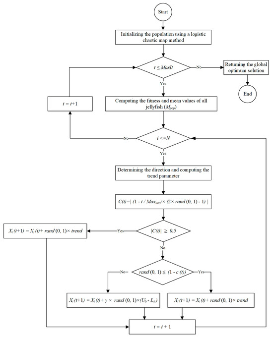
3.2. Conscious Neighborhood Concept

The neighborhood concept in the CCSA algorithm was introduced by Zamani et al. [45] to facilitate understanding of the search space and deliberate selection of movement strategies for solving global optimization problems. The CCSA comprises two strategies: Neighborhood-based Local Search (NLS) and Non-neighborhood-based Global Search (NGS), which utilize the neighborhood concept to enhance both local search and global search. During the initialization phase, a finite set of N crows (or individuals) is distributed uniformly at random across the search space. The crow ci in iteration t is shown by Equation (9), where Xi (t) and fi (t) indicate the position and the fitness of crow ci, respectively. mi(t) and fbesti show the position and best fitness of ci until the iteration t.
c i t = X i t , f i t , m i t , f b e s t i ( t )
A conscious neighborhood and non-neighborhood of ci are obtained by Equations (10) and (11), which are used to determine the movement strategy between NLS or NGS consciously, and enhance balance in the global search and local search capabilities of the algorithm. In addition, two variables, wij and µ, are calculated using Equations (12) and (13).
N ( c i ) = c j   d X i , m i × w i j < μ     f o r   j = 1 ,   ,   N   a n d   i j }
N o n N ( c i ) = c j   d X i , m i × w i j > μ     f o r   j = 1 ,   ,   N   a n d   i j }
w i j = ε + f i f b e s t j k = 1 N f i f b e s t k
μ = 1 N j = 1 N d X i , m j × w i j
where d (Xi, mj) shows the Euclidean distance between crows ci and the hiding place of crow cj. A random crow and the best crow from the neighbor and non-neighbor vicinity of crow ci are selected, named clocal and cglobal, respectively. If the fitness value of clocal is less than the fitness value of cglobal, the NLS strategy is adopted for the subsequent movement; otherwise, the NGS strategy is selected.

3.3. Wandering Around Search (WAS) Strategy

The WAS strategy analyzes the crows’ surrounding environment and changes their position through several jumps. The reason is to recalibrate the positions of crows that have not achieved better fitness values through the NLS or NGS strategies. WAS provides an additional chance for inferior individuals to improve their fitness value. Thus, inferior individuals explore the search space by accomplishing a random number of jumps (NJ), where k dimensions are randomly picked and their values are altered. The WAS strategy is defined in Equation (14).
X i j t + 1 = m g b e s t   j t + r i × f l i ( t ) × ( X r j ( t ) X i j ( t ) )
where mgbest j and Xrj(t) denote the value of dimension j for the best hiding place and a randomly chosen crow, respectively. ri is a uniformly distributed random number in the interval [0, 1], and fli(t) is the flight length of the crow ci at iteration t, which is a linearly decreasing variable and is calculated by Equation (15).
f l j = 2.02 1.08 N J × j
where the number of jumps (NJ) is randomly selected between 1 and 50, and j is from 1 to NJ.

4. Proposed Algorithm

This section describes the proposed Conscious Neighborhood-based JSO (CNJSO) algorithm. To tackle the JSO algorithm’s weaknesses, CNJSO introduces a new movement strategy named Best archive and Non-neighborhood-based Global Search, or BNGS, to enhance the exploration. It also adapts and utilizes the concept of conscious neighborhood to select between exploration and exploitation. Moreover, CNJSO employs the Wandering Around Search (WAS) strategy introduced by the CCSA algorithm [45] to improve inferior individuals. The following subsections will provide detailed explanations of how the CNJSO algorithm utilizes the introduced BNGS strategy and the WAS strategy.

4.1. Exploration Improvement Using the Introduced BNGS Strategy

Since the JSO suffers from low exploration and inconsistency between exploration and exploitation, this study introduces a new search strategy called the Best archive and Non-neighborhood-based Global Search (BNGS) strategy. In addition, the conscious neighborhood concept is employed to determine the movement strategy between the ocean’s current and the jellyfish swarm, making a good trade-off between global and local search. To consciously select the movement strategy, the neighbors and non-neighbors of each individual are determined by Equations (10) and (11). Then, an individual is randomly selected from the neighborhood set (local), and an individual with the best fitness value of the non-neighborhood set (global) is picked for individual i, denoted by Xlocal and Xglobal, respectively. If the fitness value of Xlocal (flocal) is better than the fitness value of Xglobal (fglobal), individual i moves within the jellyfish swarm; otherwise, it moves along the ocean’s current using the new BNGS search strategy to enhance the exploration of CNJSO. Moreover, the best archive is utilized to maintain the best individual generated in each iteration. The size of the archive is equal to the population size, and when it is full, some previous individuals are randomly removed from it. The introduced BNGS strategy generates new positions according to Equation (16).
X i t + 1 = X a r c h i v e ( t ) + c ( t ) × ( X i t X g l o b a l ( t ) )
where Xarchive indicates a randomly selected jellyfish from the archive, and Xglobal is a random non-neighbor of individual i. The coefficient c(t) is a time-control parameter calculated by Equation (8).

4.2. Improving Inferior Jellyfishes Using Wandering Around Search (WAS) Strategy

This study employs the Wandering Around Search (WAS) strategy to improve inferior jellyfishes. Accordingly, individual behaviors are examined, and if their current positions are unsatisfactory, they are consistently relocated to more favorable positions. Thus, the objective of WAS is to realign the positions of individuals who have not achieved a good fitness value. As a result, if the new fitness value of individual i is not better than its previous fitness value, individual i moves to another position using a random number of jumps (NJ), where k dimensions are randomly selected for each jump and their values are modified using Equation (17).
X i j t + 1 = m g b e s t   j ( t ) + r i × f l i ( t ) × ( X r j t X i j ( t ) )
where Xij (t + 1) represents the value of dimension j in the new position of individual i. mgbest j(t) and Xrj (t) denote the value of dimension j for the best and a randomly selected individual, respectively. fli (t) is a linearly decreasing variable, and ri is a random number uniformly distributed in the interval [0, 1].
Figure 2 illustrates the flowchart of the proposed CNJSO algorithm, highlighting the new components indicated by the grey boxes.
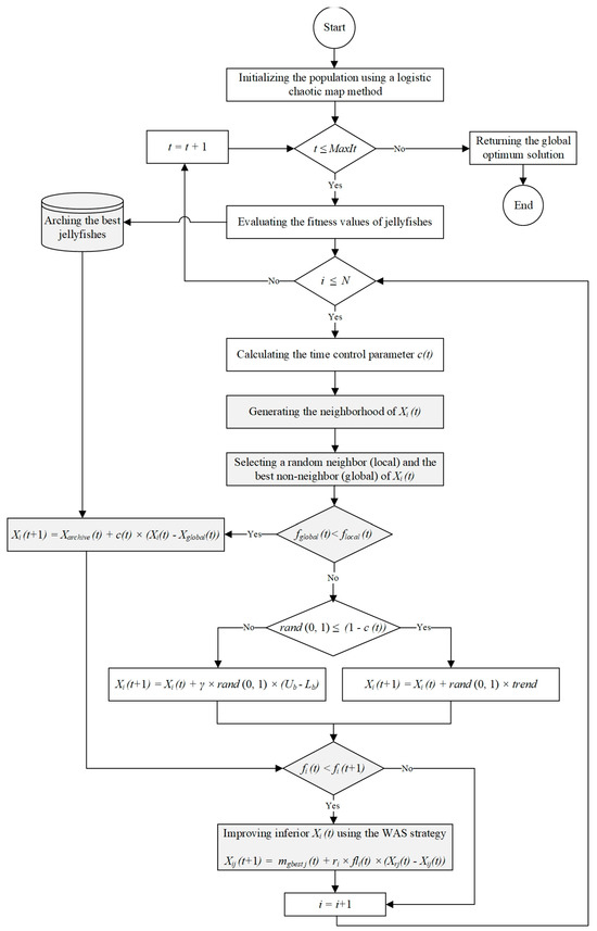
5. Experimental Evaluation and Results

In this study, the performance of CNJSO is assessed on the CEC 2018 benchmark function [50], with dimensions of 30, 50, and 100. Then, results were compared with several of the state-of-the-art swarm intelligence algorithms—PSO, KH, GWO, WOA, EEGWO, HGSO, JSO, TSA, MTBO, and FOA—and the convergence behavior of these algorithms was demonstrated. In addition, the overall performance of CNJSO and comparative algorithms was statistically examined using the Wilcoxon rank-sum and Friedman tests.

5.1. Benchmark Functions

The CEC 2018 benchmark functions, where the complexity levels progressively increase with increasing dimensionality, were used in this study. This benchmark set incorporates 29 optimization problems of various types: unimodal (F1 and F3), multimodal (F4–F10), hybrid (F11–F20), and composite (F21–F30). Because the unimodal functions have a single global optimum, they are appropriate for assessing exploitation ability. As opposed to unimodal functions, multimodal functions have numerous local optima, making them appropriate for evaluating exploration abilities. The capability to strike a balance between exploration and exploitation can be evaluated concurrently using the hybrid and composite functions.

5.2. Experimental Setup

Due to the stochastic nature of swarm intelligence algorithms, their evaluation should be conducted in an impartial setting [5], and all tests should be carefully carried out under fair conditions [106]. Therefore, CNJSO and comparative algorithms were implemented using MATLAB 2018a, and experiments were conducted on an Intel Core i7-6500U CPU (2.50 GHz) with 8 GB main memory.
To ensure fair comparisons and consistent programming approaches across all tests [50], all experiments are run 20 times, while the maximum number of iterations and the population size are set to 104 × dimension and 100, respectively. The mean error, standard deviation, and minimum (min) of the global best solution found after 20 runs are compared to assess how well an algorithm performs. Table 1 displays the parameters of the comparative algorithms.

5.3. Performance Evaluation

Different functions of the CEC 2018 benchmark are employed to evaluate the performance of CNJSO and compare it with several comparative algorithms in terms of exploration, exploitation, and ability to escape from local optima. This subsection reports the numerical results in Table 2, Table 3, Table 4 and Table 5, in which the bold letters show the best results. In the last rows of these tables, the number of wins (W), ties (T), and losses (L) is provided.

5.3.1. Evaluation of Exploitation and Exploration

The CNJSO is experimentally appraised by benchmark functions F1 and F3 on different dimensions, 30, 50, and 100. Table 2 shows the experimental results of CNJSO and comparative algorithms, which prove the strong exploitation ability of CNJSO. The benchmark functions F4–F10 have multiple local optima that increase exponentially in dimension, making them appropriate for assessing the exploration ability of CNJSO and comparative algorithms. Table 3 represents the experimental results of CNJSO and comparative algorithms to solve multimodal functions on dimensions 30, 50, and 100. Table 4 and Table 5 show the results of CNJSO and competing algorithms on test functions F11–F30, which verify the improvement in exploration and exploitation ability using the conscious neighborhood concept.
The primary reason is that this concept helps determine an effective movement strategy consciously. In this study, each individual’s neighborhood and non-neighborhood are evaluated to determine the next movement strategy rather than relying on a time-based mechanism to switch between local and global search. This approach allows the population to adaptively balance exploration and exploitation based on the current search context. Additionally, the proposed BNGS enhances CNJSO’s exploration capability through two complementary mechanisms. First, a random individual is selected from an archive containing the best-performing individuals; this allows information from high-quality solutions to influence the population and guides individuals toward promising regions in the search space. Second, a random non-neighborhood individual is selected to incorporate information from diverse areas outside the immediate neighborhood, promoting broader exploration. The combination of these two mechanisms enables CNJSO to explore the search space effectively, avoid premature convergence, and maintain a robust balance between local refinement and global search.

5.3.2. Evaluation of Escape Ability from Local Optima

To evaluate the balance between exploration and exploitation, which sets the stage for escaping from the local optima trap, the hybrid and composite functions are appropriate. The results in Table 4 indicate that the proposed CNJSO outperforms the comparative algorithms on the hybrid functions F11–F20. The results in Table 5 indicate that the CNJSO algorithm handles the composite optimization problems posed by the benchmark functions F21–F30 more effectively than the comparative algorithms, particularly at a dimensionality of 100. The primary cause for this is that the use of WAS forced those individuals who could not achieve good fitness to adjust their positions. The WAS strategy is used to examine how individuals behave, jumping to another spot if their present position is not satisfactory. Thus, this strategy can strike a balance between exploration and exploitation, thereby avoiding the risk of becoming trapped in local optima.

5.4. Convergence Analysis

The convergent curves of CNJSO and comparative algorithms are illustrated in Figure 3. Regarding these curves, it becomes evident that CNJSO reveals comparable convergence for the majority of the functions. These results demonstrate that CNJSO decreases premature convergence and improves the balance between local and global search by preserving the continuity around the local and global optima in these functions. Compared to the competing algorithms, CNJSO consistently reaches lower objective function values in fewer iterations, indicating faster and more reliable convergence. This improved performance can be attributed to CNJSO’s ability to explore the search space effectively while exploiting promising regions, thereby avoiding local traps and achieving a better approximation of the global optimum across various test functions.
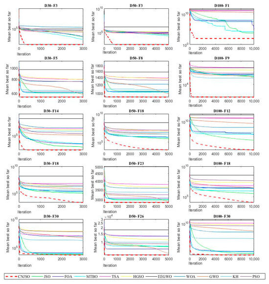
5.5. Statistical Analysis

To assess the significance of performance differences between CNJSO and competing algorithms, the non-parametric Wilcoxon rank-sum and Friedman tests were employed.

5.5.1. Non-Parametric Friedman Test

The nonparametric Friedman (Ff) test [107] evaluates whether there are significant differences in performance among two or more algorithms. For each dataset or test case, the algorithms are ranked independently, with the best-performing algorithm assigned rank one and the worst-performing algorithm assigned rank k, while ties are assigned average ranks. The final rank of each algorithm is determined by computing the average of its ranks across all datasets. The Friedman statistic Ff is calculated using Equation (18), where k is the number of algorithms, Rj is the average rank of algorithm j, and n is the number of test cases. This statistic is then compared to a chi-square distribution to test the null hypothesis that all algorithms perform equivalently. The results in Table 6 show that CNJSO outperforms the other algorithms, achieving the top overall rank.
F f = 12 n k ( k + 1 ) j R j 2 k ( k + 1 ) 2 4

5.5.2. Wilcoxon Rank-Sum

The Wilcoxon rank-sum test [108] is used to evaluate the statistical significance of CNJSO and the competitor algorithm’s results. The samples in the rank-sum experiment are assigned ranks, and the sum of the ranks is then determined. In this test, the null hypothesis (H0) states that there is no significant difference in the performance of the compared algorithms at a significance level of 0.05 when employing the benchmark functions. The p-values for dimensions 30, 50, and 100 are shown in Table 7, Table 8 and Table 9, where an underlined value indicates a p-value greater than 0.05. Thus, the results indicate that the null hypothesis is rejected for the majority of functions, and CNJSO demonstrates statistically significant improvements compared to the other algorithms.

5.6. Sensitivity Analysis

Three sets of experiments were conducted to analyze the sensitivity of the CNJSO, using population sizes of 30, 50, and 100 and varying γ values for a problem dimension of 10. Table 10 displays the experimental results of CNJSO gained for all the benchmark functions, including unimodal, multimodal, hybrid, and composite with different parameters γ, and the results of the Friedman test. In the first set of experiments, the population size was fixed at 30, and the algorithm’s performance was assessed using four different values of γ: 0.05, 0.1, 0.2, and 3.0. The results demonstrate the impact of varying the γ parameter on performance rankings, as measured using the Friedman test for a population size of 30. With γ = 0.05, the algorithm achieved the lowest rank, 4th place, indicating comparatively weaker performance. Increasing γ to 0.1 improved the results, yielding a rank of 3. At γ = 0.2, performance was further enhanced with a rank of 2, showing a consistent upward trend. Finally, at γ = 1.0, the algorithm achieved the best rank, 1st place, indicating that this setting optimizes performance under the given conditions.
For the second set of experiments, the population size was set to 50, and the algorithm was evaluated with γ values of 0.05, 0.1, 0.2, and 0.3. The results show a clear trend of improved performance with increasing γ. Specifically, with γ = 0.05, the algorithm ranked 4th, indicating the weakest performance. Increasing γ to 0.1 and 0.2 led to ranks of 3 and 2, respectively. The best performance was achieved at γ = 0.3, where the algorithm obtained the top rank, 1st place. For the third set of experiments, the population size was increased to 100, and the algorithm was tested with γ values of 0.05, 0.1, 0.2, and 0.3. The results differed from those of other comparative population sizes and revealed that the most suitable performance was obtained when γ = 0.05. Therefore, the results verify that the effect of parameter γ decreases as the population size increases. These results indicated that variations in population size and the γ coefficient influence the performance of the CNJSO algorithm.

6. Applicability of CNJSO for Solving Optimal Power Flow Problems

The Optimal Power Flow (OPF) problem is a fundamental challenge in electrical engineering, focused on optimizing the distribution of electrical power across a network. It represents a class of non-linear optimization problems that are constrained by the operational limits of the power system and the governing power flow equations [109]. This optimization ensures the network operates efficiently, adhering to various constraints, including power balance, voltage limits, and system stability. These problems are inherently complex and representative of real-world power system operations. As such, they provide a rigorous test for optimization algorithms. This section investigates the applicability of CNJSO in addressing complex OPF problems, using the IEEE 30-bus and 118-bus systems as benchmark cases.

6.1. Optimal Power Flow Problem for IEEE 30-Bus System

The IEEE 30–bus system comprises six generators, four transformers, and nine shunt VAR compensation buses. The lower and upper bounds of the transformer tap are set to 0.9 and 1.1 p.u. The minimum and maximum values of voltages for all generator buses and the shunt VAR compensations are 0.95, 1.1, 0.0, and 0.05 p.u, respectively. The schematic of the IEEE 30-bus is shown in Figure 4.
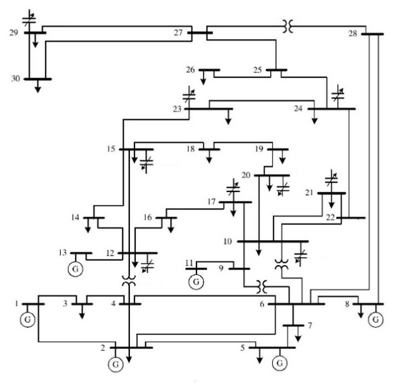
Case 1: Minimization of the fuel cost
The minimization of fuel cost for all generators is defined as the objective function f1 and is computed using Equation (19).
f 1 = i = 1 N G a i + b i P G i + c i P G i 2
where ai, bi, and ci specify the cost coefficients of the generator i. For PGi (in MW), the coefficients ai, bi, and ci are expressed in $/hr, $/MWh, and S/MW2h, respectively.
Case 2: Voltage profile improvement
The objective function f2 considers both fuel cost minimization and voltage deviation minimization and is calculated using Equation (20).
f 2 = i = 1 N G a i + b i P G i + c i P G i 2 + w v i = 1 N L V i 1.0
where the weighting factor for voltage deviation is wv, and its value is set to 200.

6.2. Optimal Power Flow Problem for IEEE 118-Bus System

The IEEE 118-bus test problem has 54 generators, 186 branches, nine transformers, two reactors, and 12 capacitors. The control variables consist of the 54 generator outputs, nine settings for transformers, and 12 shunt capacitor reactive power injections. The voltage limits of all buses are between 0.94 and 1.06 p.u. The transformer tap settings are within the interval of 0.90–1.10 p.u. The available reactive powers of shunt capacitors are considered in the range of 0–30 MVAR. Similar to Cases 1 and 2, the objectives of this problem are to minimize the total fuel cost of all generators and improve the voltage profile. The schematic of the system is shown in Figure 5.
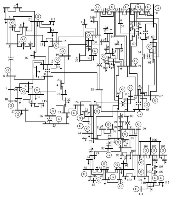
Table 11, Table 12, Table 13 and Table 14 tabulate the findings of the comparative algorithms and CNJSO to solve OPF problems. The population size, maximum number of iterations, and number of runs are set at 50, 200, and 20, respectively. The experimental results demonstrate that the proposed CNJSO algorithm outperforms the competing algorithms in addressing these engineering problems.

7. Conclusions

OPF and global optimization problems are a class of complex, nonlinear, and large-scale optimization problems that pose significant computational challenges. Although these challenges make them well-suited for metaheuristic algorithms, which are capable of efficiently exploring complex search spaces and maintaining a balance between exploration and exploitation, many existing algorithms still face limitations such as premature convergence, insufficient exploration, or an imbalance between exploration and exploitation. The JSO is a successful metaheuristic algorithm, which mimics the foraging behavior of the jellyfishes in the ocean. This algorithm suffers from low exploration and an imbalance between exploration and exploitation. To tackle these drawbacks, this study introduced an improved JSO called Conscious Neighborhood-based JSO (CNJSO), which the new movement strategy BNGS proposes to enhance search space exploration. In addition, this algorithm adapted and utilized the concept of conscious neighborhood to decide between exploration and exploitation, and employed the Wandering Around Search (WAS) strategy to improve inferior individuals. The performance of CNJSO was assessed by conducting the CEC 2018 benchmark functions, and the results were statistically analyzed. In addition, the applicability of CNJSO was evaluated by solving the optimal power flow problems for the IEEE 30-bus and 118-bus systems. To sum up, the outcomes of the experiment and analysis can be described as follows.
  • Using the conscious neighborhood concept enables the algorithm to consciously determine the movement strategy between the ocean’s current and the jellyfish swarm and makes a good trade-off between exploration and exploitation.
  • Proposing the Best archive and Non-neighborhood-based Global Search (BNGS) strategy enhances exploration ability.
  • The WAS strategy decreases premature convergence and improves the balance between local and global search.
  • The proposed CNJSO algorithm performed better than competitor algorithms for different test functions.
  • CNJSO can be used to resolve engineering design problems.
Although the proposed CNJSO has indicated superior performance on OPF problems, this study has a particular limitation. The CNJSO requires a longer execution time compared to conventional approaches, which can be a significant limitation in real-time applications. The proposed CNJSO algorithm is applied to solve single-objective and continuous problems. As future work, it can be extended to optimize binary and multi-objective problems. Since multi-objective optimization requires constructing Pareto frontiers, an external archive of non-dominated solutions can be applied. In addition, using the conscious neighborhood concept, the population can learn from different non-dominated solutions instead of a single one. Additionally, CNJSO can be utilized for solving optimization problems in various applications and domains.

Author Contributions

M.H.N.-S.: Conceptualization, methodology, software, validation, formal analysis, investigation, writing—original draft, writing—review & editing, supervision, project administration; M.B.-D.: Conceptualization, methodology, software, validation, formal analysis, investigation, writing- original draft, writing—review & editing; H.Z.: Conceptualization, methodology, software, validation, formal analysis, investigation, writing- original draft, writing—review & editing. All authors have read and agreed to the published version of the manuscript.

Funding

This research received no external funding.

Data Availability Statement

The original contributions presented in this study are included in the article. Further inquiries can be directed to the corresponding author.

Conflicts of Interest

The authors have no competing interests to declare that are relevant to the content of this article.

Nomenclature

The nomenclature table:
Variable NameDescription
t and MaxiterCurrent iteration and the maximum number of iterations
Xi(t) Position of the i-th jellyfish at time t
Xij(t + 1) The j-th dimension of the i-th jellyfish’s position
f X i Fitness value of the i-th jellyfish at time t
X*Position of the current best jellyfish in the swarm
μMean position of all jellyfish positions
γ Motion coefficient
U b   a n d   L b Upper and lower bounds of the search space
c(t) and C0Time control function and a threshold constant
mi(t) and fbestiPosition and best fitness value of the i-th jellyfish
mgbestj and Xrj(t)The j-th dimension of the best hiding place and the r-th random search agent
riA random value in the interval (0, 1)
fli(t) Flight length for the i-th search agent in the current iteration t
XarchiveA randomly selected jellyfish from the archive
XglobalA random non-neighbor of individual i
NJNumber of jumps

References

  1. Li, S.; Chen, H.; Wang, M.; Heidari, A.A.; Mirjalili, S. Slime mould algorithm: A new method for stochastic optimization. Future Gener. Comput. Syst. 2020, 111, 300–323. [Google Scholar] [CrossRef]
  2. Chen, H.; Jiao, S.; Heidari, A.A.; Wang, M.; Chen, X.; Zhao, X. An opposition-based sine cosine approach with local search for parameter estimation of photovoltaic models. Energy Convers. Manag. 2019, 195, 927–942. [Google Scholar] [CrossRef]
  3. Rashedi, E.; Nezamabadi-pour, H.; Saryazdi, S. GSA: A gravitational search algorithm. Inf. Sci. 2009, 179, 2232–2248. [Google Scholar] [CrossRef]
  4. Gandomi, A.H.; Alavi, A.H. Krill herd: A new bio-inspired optimization algorithm. Commun. Nonlinear Sci. Numer. Simul. 2012, 17, 4831–4845. [Google Scholar] [CrossRef]
  5. Talbi, E.-G. Metaheuristics: From Design to Implementation; Wiley Publishing: Hoboken, NJ, USA, 2009. [Google Scholar]
  6. Abdel-Basset, M.; Mohamed, R.; Elhoseny, M. applications. In Metaheuristics Algorithms for Medical Applications; Abdel-Basset, M., Mohamed, R., Elhoseny, M., Eds.; Academic Press: Cambridge, MA, USA, 2024; pp. 1–26. [Google Scholar] [CrossRef]
  7. Khosravy, M.; Gupta, N.; Patel, N.; Senjyu, T. Frontier Applications of Nature Inspired Computation; Springer: Singapore, 2020. [Google Scholar]
  8. Wolpert, D.H.; Macready, W.G. No free lunch theorems for optimization. IEEE Trans. Evol. Comput. 1997, 1, 67–82. [Google Scholar] [CrossRef]
  9. Mandal, P.K. A review of classical methods and Nature-Inspired Algorithms (NIAs) for optimization problems. Results Control Optim. 2023, 13, 100315. [Google Scholar] [CrossRef]
  10. Beyer, H.-G.; Schwefel, H.-P. Evolution strategies—A comprehensive introduction. Nat. Comput. 2002, 1, 3–52. [Google Scholar] [CrossRef]
  11. Grefenstette, J.J. Genetic algorithms and machine learning. In Proceedings of the Sixth Annual Conference on Computational Learning Theory, Association for Computing Machinery, Santa Cruz, CA, USA, 1 August 1993; pp. 3–4. [Google Scholar] [CrossRef]
  12. Eberhart, R.; Kennedy, J. A new optimizer using particle swarm theory. In Proceedings of the Sixth International Symposium on Micro Machine and Human Science, Nagoya, Japan, 4–6 October 1995. [Google Scholar] [CrossRef]
  13. Dorigo, M.; Caro, G.D. Ant colony optimization: A new meta-heuristic. In Proceedings of the 1999 Congress on Evolutionary Computation-CEC99 (Cat. No. 99TH8406), Washington, DC, USA, 6–9 July 1999. [Google Scholar] [CrossRef]
  14. Mirjalili, S.; Lewis, A. Grey wolf optimizer. Adv. Eng. Softw. 2014, 69, 46–61. [Google Scholar] [CrossRef]
  15. Chou, J.-S.; Truong, D.-N. A novel metaheuristic optimizer inspired by behavior of jellyfish in ocean. Appl. Math. Comput. 2021, 389, 125535. [Google Scholar] [CrossRef]
  16. Kaur, S.; Awasthi, L.K.; Sangal, A.L.; Dhiman, G. Tunicate Swarm Algorithm: A new bio-inspired based metaheuristic paradigm for global optimization. Eng. Appl. Artif. Intell. 2020, 90, 103541. [Google Scholar] [CrossRef]
  17. Hamadneh, T.; Batiha, B.; Werner, F.; Montazeri, Z.; Dehghani, M.; Gulnara, B.; Eguchi, K. Fossa Optimization Algorithm: A New Bio-Inspired Metaheuristic Algorithm for Engineering Applications. Int. J. Intell. Eng. Syst. 2024, 17, 1038–1047. [Google Scholar] [CrossRef]
  18. Rao, R.V.; Savsani, V.J.; Vakharia, D.P. Teaching–learning-based optimization: A novel method for constrained mechanical design optimization problems. Comput.-Aided Des. 2011, 43, 303–315. [Google Scholar] [CrossRef]
  19. Ida Evangeline, S.; Rathika, P. Wind farm incorporated optimal power flow solutions through multi-objective horse herd optimization with a novel constraint handling technique. Expert Syst. Appl. 2022, 194, 116544. [Google Scholar] [CrossRef]
  20. Nadimi-Shahraki, M.H.; Taghian, S.; Javaheri, D.; Sadiq, A.S.; Khodadadi, N.; Mirjalili, S. MTV-SCA: Multi-trial vector-based sine cosine algorithm. Clust. Comput. 2024, 27, 13471–13515. [Google Scholar] [CrossRef]
  21. Kaveh, A.; Kaveh, A.; Nasrollahi, A. Charged system search and particle swarm optimization hybridized for optimal design of engineering structures. Sci. Iran. 2014, 21, 295–305. [Google Scholar]
  22. Varaee, H.; Safaeian Hamzehkolaei, N.; Safari, M. A Hybrid Generalized Reduced Gradient-Based Particle Swarm Optimizer for Constrained Engineering Optimization Problems. J. Soft Comput. Civ. Eng. 2021, 5, 86–119. [Google Scholar] [CrossRef]
  23. Wu, H.; Bagherzadeh, S.A.; D’oRazio, A.; Habibollahi, N.; Karimipour, A.; Goodarzi, M.; Bach, Q.-V. Present a new multi objective optimization statistical Pareto frontier method composed of artificial neural network and multi objective genetic algorithm to improve the pipe flow hydrodynamic and thermal properties such as pressure drop and heat transfer coefficient for non-Newtonian binary fluids. Phys. A Stat. Mech. Appl. 2019, 535, 122409. [Google Scholar] [CrossRef]
  24. Abdel-Basset, M.; El-Shahat, D.; El-Henawy, I.; de Albuquerque, V.H.C.; Mirjalili, S. A new fusion of grey wolf optimizer algorithm with a two-phase mutation for feature selection. Expert Syst. Appl. 2020, 139, 112824. [Google Scholar] [CrossRef]
  25. Banaie-Dezfouli, M.; Nadimi-Shahraki, M.H.; Beheshti, Z. BE-GWO: Binary extremum-based grey wolf optimizer for discrete optimization problems. Appl. Soft Comput. 2023, 146, 110583. [Google Scholar] [CrossRef]
  26. Dezfuly, M.; Sajedi, H. Predict Survival of Patients with Lung Cancer Using an Ensemble Feature Selection Algorithm and Classification Methods in Data Mining. J. Inf. 2015, 1, 1–11. [Google Scholar] [CrossRef][Green Version]
  27. Beheshti, Z. BMPA-TVSinV: A Binary Marine Predators Algorithm using time-varying sine and V-shaped transfer functions for wrapper-based feature selection. Knowl. Based Syst. 2022, 252, 109446. [Google Scholar] [CrossRef]
  28. Ouadfel, S.; Elaziz, M.A. Efficient high-dimension feature selection based on enhanced equilibrium optimizer. Expert Syst. Appl. 2022, 187, 115882. [Google Scholar] [CrossRef]
  29. Dezfouli, M.B.; Nadimi-Shahraki, M.-H.; Zamani, H. A novel tour planning model using big data. In Proceedings of the 2018 International Conference on Artificial Intelligence and Data Processing (IDAP), New York, NY, USA, 28–30 September 2018. [Google Scholar] [CrossRef]
  30. Ghazzai, H.; Yaacoub, E.; Alouini, M.-S. Optimized LTE Cell Planning for Multiple User Density Subareas Using Meta-Heuristic Algorithms. In Proceedings of the 2014 IEEE 80th Vehicular Technology Conference (VTC2014-Fall), Vancouver, BC, Canada, 14–17 September 2014. [Google Scholar] [CrossRef]
  31. Chiang, H.-S.; Huang, T.-C. User-adapted travel planning system for personalized schedule recommendation. Inf. Fusion 2015, 21, 3–17. [Google Scholar] [CrossRef]
  32. Nadimi-Shahraki, M.H.; Moeini, E.; Taghian, S.; Mirjalili, S. Discrete Improved Grey Wolf Optimizer for Community Detection. J. Bionic Eng. 2023, 20, 2331–2358. [Google Scholar] [CrossRef]
  33. Pérez-Peló, S.; Sánchez-Oro, J.; Gonzalez-Pardo, A.; Duarte, A. A fast variable neighborhood search approach for multi-objective community detection. Appl. Soft Comput. 2021, 112, 107838. [Google Scholar] [CrossRef]
  34. Altan, A.; Karasu, S.; Bekiros, S. Digital currency forecasting with chaotic meta-heuristic bio-inspired signal processing techniques. Chaos Solitons Fractals 2019, 126, 325–336. [Google Scholar] [CrossRef]
  35. Dashti, S.E.; Rahmani, A.M. Dynamic VMs placement for energy efficiency by PSO in cloud computing. J. Exp. Theor. Artif. Intell. 2015, 28, 97–112. [Google Scholar] [CrossRef]
  36. Nadimi-Shahraki, M.H.; Banaie-Dezfouli, M.; Zamani, H.; Taghian, S.; Mirjalili, S. B-MFO: A Binary Moth-Flame Optimization for Feature Selection from Medical Datasets. Computers 2021, 10, 136. [Google Scholar] [CrossRef]
  37. Li, Q.; Chen, H.; Huang, H.; Zhao, X.; Cai, Z.; Tong, C.; Liu, W.; Tian, X. An Enhanced Grey Wolf Optimization Based Feature Selection Wrapped Kernel Extreme Learning Machine for Medical Diagnosis. Comput. Math. Methods Med. 2017, 2017, 9512741. [Google Scholar] [CrossRef]
  38. Abualigah, L.M.; Khader, A.T.; Hanandeh, E.S. A new feature selection method to improve the document clustering using particle swarm optimization algorithm. J. Comput. Sci. 2018, 25, 456–466. [Google Scholar] [CrossRef]
  39. Zhang, S.; Zhou, Y. Grey Wolf Optimizer Based on Powell Local Optimization Method for Clustering Analysis. Discret. Dyn. Nat. Soc. 2015, 2015, 481360. [Google Scholar] [CrossRef]
  40. Abasi, A.K.; Khader, A.T.; Al-Betar, M.A.; Naim, S.; Makhadmeh, S.N.; Alyasseri, Z.A.A. Link-based multi-verse optimizer for text documents clustering. Appl. Soft Comput. 2020, 87, 106002. [Google Scholar] [CrossRef]
  41. Hu, G.; Wang, J.; Li, M.; Hussien, A.G.; Abbas, M. EJS: Multi-Strategy Enhanced Jellyfish Search Algorithm for Engineering Applications. Mathematics 2023, 11, 851. [Google Scholar] [CrossRef]
  42. Lei, Y.; Fan, L.; Yang, J.; Si, W.; Lawrynczuk, M. Fractional-Order Boosted Jellyfish Search Optimizer with Gaussian Mutation for Income Forecast of Rural Resident. Comput. Intell. Neurosci. 2022, 2022, 3343505. [Google Scholar] [CrossRef]
  43. Manita, G.; Zermani, A. A Modified Jellyfish Search Optimizer with Orthogonal Learning Strategy. Procedia Comput. Sci. 2021, 192, 697–708. [Google Scholar] [CrossRef]
  44. Shaheen, A.M.; El-Sehiemy, R.A.; Alharthi, M.M.; Ghoneim, S.S.; Ginidi, A.R. Multi-objective jellyfish search optimizer for efficient power system operation based on multi-dimensional OPF framework. Energy 2021, 237, 121478. [Google Scholar] [CrossRef]
  45. Zamani, H.; Nadimi-Shahraki, M.H.; Gandomi, A.H. CCSA: Conscious Neighborhood-based Crow Search Algorithm for Solving Global Optimization Problems. Appl. Soft Comput. 2019, 85, 105583. [Google Scholar] [CrossRef]
  46. Mirjalili, S.; Lewis, A. The whale optimization algorithm. Adv. Eng. Softw. 2016, 95, 51–67. [Google Scholar] [CrossRef]
  47. Long, W.; Jiao, J.; Liang, X.; Tang, M. An exploration-enhanced grey wolf optimizer to solve high-dimensional numerical optimization. Eng. Appl. Artif. Intell. 2018, 68, 63–80. [Google Scholar] [CrossRef]
  48. Hashim, F.A.; Houssein, E.H.; Mabrouk, M.S.; Al-Atabany, W.; Mirjalili, S. Henry gas solubility optimization: A novel physics-based algorithm. Futur. Gener. Comput. Syst. 2019, 101, 646–667. [Google Scholar] [CrossRef]
  49. Faridmehr, I.; Nehdi, M.L.; Davoudkhani, I.F.; Poolad, A. Mountaineering Team-Based Optimization: A Novel Human-Based Metaheuristic Algorithm. Mathematics 2023, 11, 1273. [Google Scholar] [CrossRef]
  50. Awad, N.H.; Ali, M.Z.; Suganthan, P.N.; Liang, J.J.; Qu, B.Y. Problem Definitions and Evaluation Criteria for the CEC 2017 Special Session and Competition on Single Objective Bound Constrained Real-Parameter Numerical Optimization; Technical Report; Nanyang Technological University: Singapore, 2016. [Google Scholar]
  51. Mohamed, A.W.; Hadi, A.A.; Mohamed, A.K. Gaining-sharing knowledge based algorithm for solving optimization problems: A novel nature-inspired algorithm. Int. J. Mach. Learn. Cybern. 2019, 11, 1501–1529. [Google Scholar] [CrossRef]
  52. Askari, Q.; Younas, I.; Saeed, M. Political Optimizer: A novel socio-inspired meta-heuristic for global optimization. Knowl. Based Syst. 2020, 195, 105709. [Google Scholar] [CrossRef]
  53. Del Ser, J.; Osaba, E.; Molina, D.; Yang, X.-S.; Salcedo-Sanz, S.; Camacho, D.; Das, S.; Suganthan, P.N.; Coello, C.A.C.; Herrera, F. Bio-inspired computation: Where we stand and what’s next. Swarm Evol. Comput. 2019, 48, 220–250. [Google Scholar] [CrossRef]
  54. Koza, J.R. Genetic programming as a means for programming computers by natural selection. Stat. Comput. 1994, 4, 87–112. [Google Scholar] [CrossRef]
  55. Storn, R.; Price, K. Differential evolution—A simple and efficient heuristic for global optimization over continuous spaces. J. Glob. Optim. 1997, 11, 341–359. [Google Scholar] [CrossRef]
  56. Cuevas, E.; Zaldívar, D.; Pérez-Cisneros, M.; Oliva, D. Block-matching algorithm based on differential evolution for motion estimation. Eng. Appl. Artif. Intell. 2012, 26, 488–498. [Google Scholar] [CrossRef]
  57. Awad, N.H.; Ali, M.Z.; Mallipeddi, R.; Suganthan, P.N. An efficient Differential Evolution algorithm for stochastic OPF based active–reactive power dispatch problem considering renewable generators. Appl. Soft Comput. 2019, 76, 445–458. [Google Scholar] [CrossRef]
  58. Salman, A.; Engelbrecht, A.P.; Omran, M.G. Empirical analysis of self-adaptive differential evolution. Eur. J. Oper. Res. 2007, 183, 785–804. [Google Scholar] [CrossRef]
  59. Zhang, J. and A.C. Sanderson, JADE: Adaptive differential evolution with optional external archive. IEEE Trans. Eviron. Comp. 2009, 13, 945–958. [Google Scholar] [CrossRef]
  60. Tanabe, R.; Fukunaga, A. Success-history based parameter adaptation for Differential Evolution. In Proceedings of the 2013 IEEE Congress on Evolutionary Computation, Cancun, Mexico, 20–23 June 2013. [Google Scholar] [CrossRef]
  61. Tanabe, R.; Fukunaga, A.S. Improving the search performance of SHADE using linear population size reduction. In Proceedings of the 2014 IEEE Congress on Evolutionary Computation (CEC), Beijing, China, 6–11 July 2014. [Google Scholar] [CrossRef]
  62. Brest, J.; Maučec, M.S.; Bošković, B. iL-SHADE: Improved L-SHADE algorithm for single objective real-parameter optimization. In Proceedings of the 2016 IEEE Congress on Evolutionary Computation (CEC), Vancouver, BC, Canada, 24–29 July 2016. [Google Scholar] [CrossRef]
  63. Meng, Z.; Pan, J.-S. Quasi-affine transformation evolution with external archive (QUATRE-EAR): An enhanced structure for differential evolution. Knowl. Based Sys. 2018, 155, 35–53. [Google Scholar] [CrossRef]
  64. Nadimi-Shahraki, M.H.; Taghian, S.; Mirjalili, S.; Faris, H. MTDE: An effective multi-trial vector-based differential evolution algorithm and its applications for engineering design problems. App. Soft Comp. 2020, 97, 106761. [Google Scholar] [CrossRef]
  65. Erol, O.K.; Eksin, I. A new optimization method: Big Bang–Big Crunch. Adv. Eng. Softw. 2006, 37, 106–111. [Google Scholar] [CrossRef]
  66. Kaveh, A.; Talatahari, S. Charged system search for optimal design of frame structures. Appl. Soft Comput. 2012, 12, 382–393. [Google Scholar] [CrossRef]
  67. Hatamlou, A. Black hole: A new heuristic optimization approach for data clustering. Inf. Sci. 2013, 222, 175–184. [Google Scholar] [CrossRef]
  68. Zhao, W.; Wang, L.; Zhang, Z. Atom search optimization and its application to solve a hydrogeologic parameter estimation problem. Knowl. Based Syst. 2019, 163, 283–304. [Google Scholar] [CrossRef]
  69. Kaveh, A.; Khayatazad, M. A new meta-heuristic method: Ray Optimization. Comput. Struct. 2012, 112–113, 283–294. [Google Scholar] [CrossRef]
  70. Kaveh, A.; Khayatazad, M. Ray optimization for size and shape optimization of truss structures. Comput. Struct. 2013, 117, 82–94. [Google Scholar] [CrossRef]
  71. Kaur, A.; Kumar, Y. A new metaheuristic algorithm based on water wave optimization for data clustering. Evol. Intell. 2021, 15, 759–783. [Google Scholar] [CrossRef]
  72. Alatas, B. A novel chemistry based metaheuristic optimization method for mining of classification rules. Expert Syst. Appl. 2012, 39, 11080–11088. [Google Scholar] [CrossRef]
  73. Ghasemi, M.R.; Varaee, H. A fast multi-objective optimization using an efficient ideal gas molecular movement algorithm. Eng. Comput. 2016, 33, 477–496. [Google Scholar] [CrossRef]
  74. Wang, H.; Chen, S.; Luo, L. A diffusion algorithm based on P systems for continuous global optimization. J. Comput. Sci. 2020, 44, 101112. [Google Scholar] [CrossRef]
  75. Yang, B.; Zhang, M.; Zhang, X.; Wang, J.; Shu, H.; Li, S.; He, T.; Yang, L.; Yu, T. Fast atom search optimization based MPPT design of centralized thermoelectric generation system under heterogeneous temperature difference. J. Clean. Prod. 2020, 248, 119301. [Google Scholar] [CrossRef]
  76. Korashy, A.; Kamel, S.; Houssein, E.H.; Jurado, F.; Hashim, F.A. Development and application of evaporation rate water cycle algorithm for optimal coordination of directional overcurrent relays. Expert Syst. Appl. 2021, 185, 115538. [Google Scholar] [CrossRef]
  77. Al-Betar, M.A.; Awadallah, M.A.; Abu Zitar, R.; Assaleh, K. Economic load dispatch using memetic sine cosine algorithm. J. Ambient. Intell. Humaniz. Comput. 2022, 14, 11685–11713. [Google Scholar] [CrossRef]
  78. Eslami, M.; Neshat, M.; Khalid, S.A. A Novel Hybrid Sine Cosine Algorithm and Pattern Search for Optimal Coordination of Power System Damping Controllers. Sustainability 2022, 14, 541. [Google Scholar] [CrossRef]
  79. Abdel-Mawgoud, H.; Kamel, S.; Khasanov, M.; Khurshaid, T. A strategy for PV and BESS allocation considering uncertainty based on a modified Henry gas solubility optimizer. Electr. Power Syst. Res. 2021, 191, 106886. [Google Scholar] [CrossRef]
  80. Hashim, F.A.; Houssein, E.H.; Hussain, K.; Mabrouk, M.S.; Al-Atabany, W. A modified Henry gas solubility optimization for solving motif discovery problem. Neural Comput. Appl. 2019, 32, 10759–10771. [Google Scholar] [CrossRef]
  81. Moosavi, S.; Bardsiri, S.H.; Khatibi, V. Poor and rich optimization algorithm: A new human-based and multi populations algorithm. Eng. Appl. Artif. Intell. 2019, 86, 165–181. [Google Scholar] [CrossRef]
  82. Mousavirad, S.J.; Ebrahimpour-Komleh, H. Human mental search: A new population-based metaheuristic optimization algorithm. Appl. Intell. 2017, 47, 850–887. [Google Scholar] [CrossRef]
  83. Dehghani, M.; Mardaneh, M.; Guerrero, J.M.; Malik, O.P.; Ramirez-Mendoza, R.A.; Matas, J.; Vasquez, J.C.; Parra-Arroyo, L. A New “Doctor and Patient” Optimization Algorithm: An Application to Energy Commitment Problem. Appl. Sci. 2020, 10, 5791. [Google Scholar] [CrossRef]
  84. Chen, X.; Xu, B.; Mei, C.; Ding, Y.; Li, K. Teaching–learning–based artificial bee colony for solar photovoltaic parameter estimation. Appl. Energy 2018, 212, 1578–1588. [Google Scholar] [CrossRef]
  85. Al-Betar, M.A.; Alyasseri, Z.A.A.; Awadallah, M.A.; Abu Doush, I. Coronavirus herd immunity optimizer (CHIO). Neural Comput. Appl. 2020, 33, 5011–5042. [Google Scholar] [CrossRef]
  86. Karaboga, D.; Basturk, B. A powerful and efficient algorithm for numerical function optimization: Artificial bee colony (ABC) algorithm. J. Glob. Optim. 2007, 39, 459–471. [Google Scholar] [CrossRef]
  87. Askarzadeh, A. A novel metaheuristic method for solving constrained engineering optimization problems: Crow search algorithm. Comput. Struct. 2016, 169, 1–12. [Google Scholar] [CrossRef]
  88. Heidari, A.A.; Mirjalili, S.; Faris, H.; Aljarah, I.; Mafarja, M.; Chen, H. Harris hawks optimization: Algorithm and applications. Futur. Gener. Comput. Syst. 2019, 97, 849–872. [Google Scholar] [CrossRef]
  89. Arora, S.; Singh, S. Butterfly optimization algorithm: A novel approach for global optimization. Soft Comput. 2018, 23, 715–734. [Google Scholar] [CrossRef]
  90. Mirjalili, S.; Gandomi, A.H.; Mirjalili, S.Z.; Saremi, S.; Faris, H.; Mirjalili, S.M. Salp Swarm Algorithm: A bio-inspired optimizer for engineering design problems. Adv. Eng. Softw. 2017, 114, 163–191. [Google Scholar] [CrossRef]
  91. Gandomi, A.H.; Yang, X.-S.; Alavi, A.H. Cuckoo search algorithm: A metaheuristic approach to solve structural optimization problems. Eng. Comput. 2012, 29, 245. [Google Scholar] [CrossRef]
  92. Mirjalili, S. The Ant Lion Optimizer. Adv. Eng. Softw. 2015, 83, 80–98. [Google Scholar] [CrossRef]
  93. Faris, H.; Aljarah, I.; Alqatawna, J. Optimizing Feedforward neural networks using Krill Herd algorithm for E-mail spam detection. In Proceedings of the 2015 IEEE Jordan Conference on Applied Electrical Engineering and Computing Technologies (AEECT), The Dead Sea, Jordan, 3–5 November 2015; pp. 1–5. [Google Scholar] [CrossRef]
  94. Thaher, T.; Heidari, A.A.; Mafarja, M.; Dong, J.S.; Mirjalili, S. Binary Harris Hawks optimizer for high-dimensional, low sample size feature selection. In Evolutionary Machine Learning Techniques; Springer: Singapore, 2020; pp. 251–272. [Google Scholar] [CrossRef]
  95. Shi, Y.; Pun, C.-M.; Hu, H.; Gao, H. An improved artificial bee colony and its application. Knowl. Based Syst. 2016, 107, 14–31. [Google Scholar] [CrossRef]
  96. Banaie-Dezfouli, M.; Nadimi-Shahraki, M.H.; Beheshti, Z. R-GWO: Representative-based grey wolf optimizer for solving engineering problems. App. Sof. Com. 2021, 106, 107328. [Google Scholar] [CrossRef]
  97. Li, X.; Yi, P.; Jiang, Y.; Zhang, F. An Improved Salp Swarm Algorithm Based on Cosine Decline and Chaos Crossover Strategies. In Proceedings of the 2020 IEEE 6th International Conference on Computer and Communications (ICCC), Chengdu, China, 11–14 December 2020. [Google Scholar] [CrossRef]
  98. Saxena, A.; Soni, B.P.; Kumar, R.; Gupta, V. Intelligent Grey Wolf Optimizer—Development and application for strategic bidding in uniform price spot energy market. Appl. Soft Comput. 2018, 69, 1–13. [Google Scholar] [CrossRef]
  99. Jayabarathi, T.; Raghunathan, T.; Adarsh, B.R.; Suganthan, P.N. Economic dispatch using hybrid grey wolf optimizer. Energy 2016, 111, 630–641. [Google Scholar] [CrossRef]
  100. Nadimi-Shahraki, M.H.; Taghian, S.; Zamani, H.; Mirjalili, S.; Elaziz, M.A.; Oliva, D. MMKE: Multi-trial vector-based monkey king evolution algorithm and its applications for engineering optimization problems. PLoS ONE 2023, 18, e0280006. [Google Scholar] [CrossRef] [PubMed]
  101. Nayyef, H.M.; Ibrahim, A.A.; Zainuri, M.A.A.M.; Zulkifley, M.A.; Shareef, H. A Novel Hybrid Algorithm Based on Jellyfish Search and Particle Swarm Optimization. Mathematics 2023, 11, 3210. [Google Scholar] [CrossRef]
  102. Kuo, R.; Chiu, T.-H. Hybrid of jellyfish and particle swarm optimization algorithm-based support vector machine for stock market trend prediction. Appl. Soft Comput. 2024, 154, 111394. [Google Scholar] [CrossRef]
  103. Yuan, X.; Hu, G.; Zhong, J.; Wei, G. HBWO-JS: Jellyfish search boosted hybrid beluga whale optimization algorithm for engineering applications. J. Comput. Des. Eng. 2023, 10, 1615–1656. [Google Scholar] [CrossRef]
  104. Mariottini, G.L.; Pane, L. Mediterranean Jellyfish Venoms: A Review on Scyphomedusae. Mar. Drugs 2010, 8, 1122–1152. [Google Scholar] [CrossRef]
  105. Zavodnik, D. Spatial aggregations of the swarming jellyfish Pelagia noctiluca (Scyphozoa). Mar. Biol. 1987, 94, 265–269. [Google Scholar] [CrossRef]
  106. Dhaenens, C.; Jourdan, L. Metaheuristics for Big Data; Wiley: Hoboken, NJ, USA, 2016; pp. i–xvi. [Google Scholar] [CrossRef]
  107. Derrac, J.; García, S.; Molina, D.; Herrera, F. A practical tutorial on the use of nonparametric statistical tests as a methodology for comparing evolutionary and swarm intelligence algorithms. Swarm Evol. Comput. 2011, 1, 3–18. [Google Scholar] [CrossRef]
  108. Wilcoxon, F. Individual comparisons by ranking methods. In Breakthroughs in Statistics: Methodology and Distribution; Kotz, S., Johnson, N.L., Eds.; Springer: New York, NY, USA, 1992; pp. 196–202. [Google Scholar] [CrossRef]
  109. Yang, Z.; Zhong, H.; Xia, Q.; Kang, C. Fundamental Review of the OPF Problem: Challenges, Solutions, and State-of-the-Art Algorithms. J. Energy Eng. 2017, 144, 04017075. [Google Scholar] [CrossRef]
Figure 1. The flowchart of the JSO algorithm.
Mathematics 13 03068 g001
Figure 2. The flowchart of the proposed CNJSO algorithm.
Mathematics 13 03068 g002
Figure 3. Comparison of convergence behavior of CNJSO and competing algorithms.
Mathematics 13 03068 g003
Figure 4. IEEE 30-bus test system single-line diagram.
Mathematics 13 03068 g004
Figure 5. IEEE 118-bus test system single-line diagram.
Mathematics 13 03068 g005
Table 1. Parameter settings.
AlgorithmsSettings
PSO [12]c1 = c2 = 2
KH [4]Vf = 0.02, Dmax = 0.005, Nmax = 0.01, Sr = 0
GWO [14]a = [2 to 0]
WOA [46]a =2, b = 1
EEGWO [47]b1 = 0.1, b2 = 0.9, mo = 1.5, ainitial = 2, afinal = 0
HGSO [48]l1 = 5 × 10⁻³, l2 = 100, l3 = 1 × 10⁻², alpha = 1, beta = 1, M1 = 0.1, M2 = 0.2
JSO [15]C0 = 0.5
TSA [16]Pmin = 1, Pmax = 4
MTBO [49]Li ∼ U [0.25, 0.50], Ai ∼ U [0.75, 1.00], Mi ∼ U [0.75, 1.00]
FOA [17]alpha = 2, beta = 1.5, gamma = 0.5, ground = 0.3, tree = 0.4, ambush = 0.3
CNJSOC0 = 0.5
Table 2. Comparison of the obtained results from unimodal test functions.
FDIndexPSO
1997
KH
2012
GWO
2014
WOA
2016
EEGWO
2018
HGSO
2019
JSO
2020
TSA
2020
MTBO
2023
FOA
2024
CNJSO
F130Min2.54 × 1088.27 × 1021.68 × 1077.79 × 1055.20 × 10103.64 × 1086.19 × 1017.49 × 1095.68 × 1014.97 × 1011.00 × 102
Mean1.54 × 10101.59 × 1048.49 × 1083.26 × 1065.97 × 10101.52 × 10101.69 × 1031.57 × 10103.66 × 1036.36 × 1034.97 × 1015
SD2.14 × 1081.31 × 1032.84 × 1072.38 × 1064.57 × 1093.77 × 1081.65 × 1036.66 × 1094.44 × 1035.91 × 1038.63 × 1015
50Min1.94 × 1081.55 × 1033.41 × 1072.53 × 1061.05 × 10113.83 × 1084.99 × 1012.45 × 10105.27 × 1012.46 × 1021.00 × 102
Mean3.78 × 10102.31 × 1054.06 × 1099.72 × 1061.16 × 10113.95 × 10101.23 × 1034.06 × 10103.11 × 1038.91 × 1032.42 × 1014
SD1.54 × 1082.04 × 1034.57 × 1071.16 × 1074.56 × 1093.96 × 1081.69 × 1039.82 × 1093.41 × 1038.13 × 1031.53 × 1014
100Min1.13 × 10112.18 × 1062.23 × 10101.77 × 1072.58 × 10111.28 × 10114.88 × 1027.85 × 10109.15 × 1011.24 × 1021.00 × 102
Mean1.29 × 10111.11 × 1083.27 × 10103.03 × 1072.70 × 10111.60 × 10115.67 × 1031.09 × 10111.63 × 1047.77 × 1042.44 × 1012
SD8.14 × 1092.59 × 1086.88 × 1098.33 × 1066.94 × 1091.65 × 10103.76 × 1031.54 × 10102.71 × 1041.42 × 1058.57 × 1012
F330Min7.40 × 1073.01 × 1036.87 × 1074.94 × 1047.58 × 1044.22 × 1082.26 × 1032.55 × 1046.31 × 1012.66 × 1023.00 × 102
Mean4.91 × 1044.53 × 1042.83 × 1041.67 × 1058.88 × 1043.84 × 1044.19 × 1034.42 × 1041.65 × 1035.46 × 1031.99 × 1014
SD3.41 × 1073.49 × 1038.03 × 1077.80 × 1044.85 × 1034.34 × 1089.34 × 1021.26 × 1041.14 × 1033.00 × 1033.45 × 1014
50Min1.41 × 1073.74 × 1038.60 × 1074.40 × 1042.15 × 1054.41 × 1082.08 × 1043.74 × 1047.28 × 1031.55 × 1043.00 × 102
Mean1.07 × 1051.15 × 1056.57 × 1047.50 × 1041.41 × 1061.39 × 1052.94 × 1048.54 × 1041.89 × 1044.24 × 1045.68 × 1014
SD2.8 × 1074.22 × 1039.76 × 1072.97 × 1043.19 × 1064.53 × 1085.12 × 1032.06 × 1048.13 × 1031.42 × 1040
100Min3.09 × 1052.53 × 1051.60 × 1053.84 × 1053.19 × 1052.50 × 1051.33 × 1051.51 × 1059.62 × 1041.92 × 1053.00 × 102
Mean3.75 × 1053.58 × 1051.98 × 1056.03 × 1057.39 × 1062.92 × 1051.61 × 1051.94 × 1051.57 × 1052.39 × 1051.65 × 1013
SD3.23 × 1045.71 × 1042.28 × 1041.74 × 1052.25 × 1072.07 × 1041.04 × 1042.74 × 1043.68 × 1042.45 × 1045.83 × 1014
Rank30W/T/L0/0/20/0/20/0/20/0/20/0/20/0/20/0/20/0/20/0/20/0/22/0/0
50W/T/L0/0/20/0/20/0/20/0/20/0/20/0/20/0/20/0/20/0/20/0/22/0/0
100W/T/L0/0/20/0/20/0/20/0/20/0/20/0/20/0/20/0/20/0/20/0/22/0/0
Table 3. Comparison of the obtained results from multimodal test functions.
FDIndexPSO
1997
KH
2012
GWO
2014
WOA
2016
EEGWO
2018
HGSO
2019
JSO
2020
TSA
2020
MTBO
2023
FOA
2024
CNJSO
F430Min5.32 × 1026.83 × 1019.37 × 1017.85 × 1011.27 × 1041.06 × 1036.78 × 1012.95 × 1024.06 × 1004.26 × 1034.00 × 102
Mean9.08 × 1029.87 × 1011.45 × 1021.59 × 1021.86 × 1041.63 × 1039.66 × 1012.32 × 1036.43 × 1014.78 × 1017.53 × 100
SD1.57 × 1022.03 × 1013.13 × 1014.22 × 1012.81 × 1034.48 × 1022.05 × 1011.89 × 1032.94 × 1013.92 × 1011.85 × 101
50Min2.28 × 1037.32 × 1012.08 × 1022.10 × 1023.12 × 1044.51 × 1037.48 × 1012.44 × 1036.30 × 1022.85 × 1014.00 × 102
Mean3.38 × 1031.54 × 1024.12 × 1022.81 × 1023.95 × 1047.71 × 1031.41 × 1026.87 × 1039.44 × 1017.22 × 1012.93 × 101
SD4.21 × 1025.06 × 1011.67 × 1025.53 × 1012.71 × 1031.78 × 1033.94 × 1012.77 × 1034.87 × 1015.27 × 1014.51 × 101
100Min1.20 × 1042.20 × 1021.82 × 1033.81 × 1029.01 × 1041.97 × 1042.65 × 1028.60 × 1031.95 × 1021.59 × 1024.00 × 102
Mean1.39 × 1043.56 × 1022.60 × 1035.35 × 1021.12 × 1052.91 × 1043.19 × 1021.59 × 1042.85 × 1022.28 × 1021.40 × 100
SD1.05 × 1035.31 × 1015.09 × 1027.35 × 1011.03 × 1045.63 × 1033.84 × 1014.83 × 1035.62 × 1013.65 × 1011.95 × 100
F530Min2.07 × 1029.06 × 1014.71 × 1011.79 × 1024.39 × 1022.56 × 1027.56 × 1011.83 × 1026.47 × 1016.77 × 1015.30 × 102
Mean2.54 × 1021.37 × 1029.17 × 1012.64 × 1024.68 × 1023.06 × 1021.07 × 1022.95 × 1021.06 × 1021.18 × 1025.80 × 101
SD2.00 × 1013.14 × 1013.30 × 1015.46 × 1011.73 × 1011.71 × 1011.78 × 1014.84 × 1012.22 × 1013.35 × 1011.34 × 101
50Min4.97 × 1022.09 × 1021.21 × 1022.73 × 1026.70 × 1024.80 × 1022.11 × 1024.62 × 1021.73 × 1021.51 × 1025.76 × 102
Mean5.31 × 1022.56 × 1021.82 × 1024.06 × 1027.45 × 1025.45 × 1022.82 × 1025.93 × 1022.36 × 1022.45 × 1021.29 × 102
SD1.76 × 1013.11 × 1013.73 × 1017.60 × 1012.63 × 1012.80 × 1014.41 × 1016.85 × 1014.18 × 1014.75 × 1013.57 × 101
100Min1.17 × 1036.21 × 1023.73 × 1027.81 × 1021.64 × 1031.22 × 1036.63 × 1021.24 × 1035.84 × 1024.64 × 1027.90 × 102
Mean1.23 × 1037.34 × 1025.68 × 1029.42 × 1021.69 × 1031.31 × 1037.52 × 1021.49 × 1036.64 × 1026.05 × 1023.57 × 102
SD2.40 × 1018.43 × 1011.49 × 1028.89 × 1011.77 × 1014.21 × 1016.11 × 1011.35 × 1025.12 × 1018.89 × 1015.64 × 101
F630Min3.53 × 1011.95 × 1011.14 × 1005.02 × 1019.61 × 1014.73 × 1014.13 × 1012.58 × 1014.94 × 1008.82 × 1006.00 × 102
Mean4.09 × 1013.55 × 1014.10 × 1006.65 × 1011.04 × 1026.48 × 1012.30 × 1006.39 × 1011.45 × 1011.99 × 1011.14 × 1013
SD2.80 × 1009.06 × 1001.86 × 1008.97 × 1005.08 × 1006.35 × 1001.84 × 1001.58 × 1016.16 × 1007.66 × 1000
50Min4.33 × 1013.74 × 1015.50 × 1006.58 × 1011.06 × 1027.14 × 1016.64 × 1006.62 × 1011.80 × 1012.70 × 1016.00 × 102
Mean5.31 × 1015.13 × 1011.05 × 1017.68 × 1011.15 × 1028.24 × 1011.35 × 1018.99 × 1012.90 × 1013.66 × 1019.66 × 1014
SD3.67 × 1006.46 × 1003.91 × 1009.80 × 1003.06 × 1004.74 × 1006.19 × 1001.49 × 1016.82 × 1007.33 × 1001.08 × 1013
100Min6.41 × 1015.14 × 1011.93 × 1017.06 × 1011.14 × 1028.68 × 1012.66 × 1018.40 × 1013.83 × 1013.71 × 1016.00 × 102
Mean7.19 × 1015.66 × 1012.72 × 1018.04 × 1011.19 × 1029.46 × 1013.84 × 1011.06 × 1024.82 × 1014.89 × 1011.59 × 1013
SD4.36 × 1003.79 × 1004.54 × 1008.76 × 1002.11 × 1003.86 × 1005.44 × 1001.27 × 1015.18 × 1007.45 × 1001.04 × 1013
F730Min6.21 × 1028.34 × 1017.15 × 1013.37 × 1026.80 × 1023.24 × 1028.09 × 1013.40 × 1028.87 × 1011.05 × 1027.53 × 102
Mean8.27 × 1021.33 × 1021.26 × 1024.90 × 1027.60 × 1024.01 × 1021.26 × 1024.91 × 1021.59 × 1021.82 × 1028.22 × 101
SD9.68 × 1012.64 × 1013.14 × 1011.04 × 1024.01 × 1013.32 × 1011.82 × 1018.58 × 1015.81 × 1015.48 × 1011.63 × 101
50Min1.61 × 1032.74 × 1022.07 × 1027.66 × 1021.28 × 1037.17 × 1021.76 × 1028.59 × 1022.37 × 1022.94 × 1028.26 × 102
Mean2.01 × 1033.62 × 1023.35 × 1029.95 × 1021.38 × 1038.29 × 1023.32 × 1029.97 × 1023.62 × 1024.45 × 1021.80 × 102
SD2.50 × 1025.66 × 1018.59 × 1017.36 × 1014.11 × 1016.43 × 1018.16 × 1019.29 × 1017.01 × 1011.05 × 1023.86 × 101
100Min4.46 × 1031.16 × 1038.50 × 1022.38 × 1033.27 × 1032.03 × 1037.04 × 1022.33 × 1031.01 × 1031.41 × 1031.10 × 103
Mean5.68 × 1031.43 × 1031.02 × 1032.56 × 1033.38 × 1032.45 × 1031.21 × 1032.62 × 1031.40 × 1031.84 × 1035.54 × 102
SD6.91 × 1021.69 × 1021.11 × 1021.04 × 1024.25 × 1011.61 × 1022.24 × 1021.82 × 1022.65 × 1022.38 × 1021.33 × 102
F830Min2.36 × 1027.36 × 1015.75 × 1011.28 × 1023.22 × 1022.27 × 1026.77 × 1012.04 × 1026.07 × 1015.07 × 1018.34 × 102
Mean2.65 × 1021.09 × 1027.64 × 1012.08 × 1023.79 × 1022.53 × 1029.49 × 1012.73 × 1028.46 × 1011.02 × 1025.37 × 101
SD1.30 × 1011.69 × 1011.46 × 1014.75 × 1011.83 × 1011.36 × 1011.66 × 1015.52 × 1012.34 × 1013.53 × 1011.46 × 101
50Min4.98 × 1022.09 × 1021.36 × 1022.93 × 1027.05 × 1025.03 × 1021.80 × 1024.48 × 1021.68 × 1021.26 × 1028.82 × 102
Mean5.25 × 1022.84 × 1021.96 × 1024.15 × 1027.69 × 1025.71 × 1022.45 × 1025.84 × 1022.23 × 1022.40 × 1021.25 × 102
SD1.81 × 1014.77 × 1013.16 × 1017.35 × 1012.16 × 1012.75 × 1013.82 × 1018.61 × 1012.85 × 1016.73 × 1012.45 × 101
100Min1.11 × 1036.85 × 1024.84 × 1028.76 × 1021.81 × 1031.30 × 1035.74 × 1021.34 × 1036.00 × 1025.24 × 1021.03 × 103
Mean1.22 × 1037.85 × 1025.49 × 1021.06 × 1031.87 × 1031.43 × 1037.54 × 1021.55 × 1037.19 × 1026.49 × 1023.60 × 102
SD4.72 × 1015.99 × 1014.79 × 1011.16 × 1022.45 × 1017.01 × 1011.37 × 1021.19 × 1027.51 × 1018.74 × 1017.74 × 101
F930Min4.31 × 1039.31 × 1029.54 × 1012.61 × 1031.08 × 1043.17 × 1038.91 × 1003.77 × 1037.62 × 1013.27 × 1029.01 × 102
Mean5.09 × 1032.31 × 1035.41 × 1025.93 × 1031.27 × 1044.98 × 1031.26 × 1028.95 × 1033.08 × 1021.27 × 1039.24 × 100
SD5.20 × 1026.62 × 1024.41 × 1021.99 × 1031.04 × 1039.90 × 1021.55 × 1022.76 × 1032.42 × 1026.25 × 1021.22 × 101
50Min1.15 × 1047.64 × 1031.51 × 1031.12 × 1043.75 × 1042.05 × 1042.92 × 1022.02 × 1041.18 × 1032.18 × 1039.10 × 102
Mean1.36 × 1049.41 × 1034.57 × 1031.95 × 1044.41 × 1042.61 × 1041.21 × 1033.31 × 1043.52 × 1035.53 × 1037.28 × 101
SD1.29 × 1031.36 × 1033.26 × 1034.97 × 1032.77 × 1032.02 × 1035.71 × 1029.11 × 1033.21 × 1033.02 × 1037.31 × 101
100Min3.25 × 1041.95 × 1041.03 × 1042.35 × 1047.64 × 1045.87 × 1048.93 × 1036.93 × 1047.02 × 1031.72 × 1041.09 × 103
Mean4.27 × 1042.19 × 1042.26 × 1043.76 × 1048.81 × 1046.45 × 1042.67 × 1048.96 × 1042.97 × 1043.12 × 1049.57 × 102
SD5.17 × 1031.59 × 1038.71 × 1031.31 × 1044.09 × 1033.26 × 1039.08 × 1031.65 × 1041.15 × 1046.88 × 1035.29 × 102
F1030Min6.54 × 1033.37 × 1031.86 × 1033.83 × 1037.17 × 1035.10 × 1032.55 × 1034.51 × 1031.79 × 1033.04 × 1031.94 × 103
Mean6.98 × 1034.06 × 1032.85 × 1035.23 × 1038.40 × 1035.72 × 1034.67 × 1035.58 × 1035.95 × 1034.42 × 1031.89 × 103
SD1.97 × 1024.36 × 1025.55 × 1026.40 × 1024.65 × 1023.44 × 1021.34 × 1034.49 × 1021.83 × 1036.32 × 1025.55 × 102
50Min1.24 × 1045.33 × 1034.23 × 1037.51 × 1031.47 × 1041.08 × 1044.57 × 1039.07 × 1035.01 × 1036.14 × 1033.83 × 103
Mean1.34 × 1046.65 × 1035.63 × 1039.07 × 1031.54 × 1041.17 × 1045.87 × 1031.07 × 1041.01 × 1048.72 × 1033.96 × 103
SD5.11 × 1028.55 × 1026.94 × 1021.30 × 1033.69 × 1026.84 × 1021.27 × 1038.93 × 1023.75 × 1039.64 × 1026.36 × 102
100Min2.95 × 1041.27 × 1041.16 × 1041.52 × 1043.01 × 1042.27 × 1041.17 × 1042.24 × 1041.15 × 1041.58 × 1049.83 × 103
Mean3.01 × 1041.45 × 1041.31 × 1041.98 × 1043.28 × 1042.50 × 1041.59 × 1042.58 × 1042.01 × 1042.11 × 1041.08 × 104
SD3.58 × 1021.30 × 1031.09 × 1031.92 × 1039.59 × 1027.73 × 1023.81 × 1031.28 × 1038.02 × 1032.39 × 1039.24 × 102
Rank30W/T/L0/0/70/0/70/0/70/0/70/0/70/0/70/0/70/0/70/0/70/0/77/0/0
50W/T/L0/0/70/0/70/0/70/0/70/0/70/0/70/0/70/0/70/0/70/0/77/0/0
100W/T/L0/0/70/0/70/0/70/0/70/0/70/0/70/0/70/0/70/0/70/0/77/0/0
Table 4. Comparison of the obtained results from hybrid test functions.
FDIndexPSO
1997
KH
2012
GWO
2014
WOA
2016
EEGWO
2018
HGSO
2019
JSO
2020
TSA
2020
MTBO
2023
FOA
2024
CNJSO
F1130Min1.25 × 1031.56 × 1021.48 × 1021.96 × 1024.30 × 1035.80 × 1023.29 × 1013.17 × 1025.00 × 1012.59 × 1011.13 × 103
Mean1.83 × 1034.02 × 1023.18 × 1023.24 × 1021.07 × 1041.44 × 1036.23 × 1013.84 × 1031.03 × 1021.29 × 1024.18 × 101
SD3.52 × 1021.84 × 1022.01 × 1027.52 × 1012.42 × 1035.84 × 1021.97 × 1012.02 × 1033.27 × 1014.55 × 1011.85 × 101
50Min3.96 × 1031.29 × 1033.63 × 1023.39 × 1021.98 × 1042.51 × 1038.88 × 1017.98 × 1031.30 × 1021.07 × 1021.15 × 103
Mean5.23 × 1033.56 × 1031.23 × 1035.00 × 1022.44 × 1044.89 × 1031.32 × 1021.20 × 1041.71 × 1021.95 × 1028.65 × 101
SD8.86 × 1021.69 × 1039.45 × 1021.02 × 1021.80 × 1031.25 × 1032.42 × 1012.24 × 1034.08 × 1014.39 × 1012.19 × 101
100Min3.72 × 1044.80 × 1041.46 × 1044.36 × 1032.39 × 1051.13 × 1055.71 × 1023.67 × 1049.46 × 1027.75 × 1021.20 × 103
Mean4.53 × 1047.37 × 1043.74 × 1046.56 × 1036.61 × 1061.31 × 1056.86 × 1025.98 × 1041.35 × 1031.05 × 1031.76 × 102
SD5.27 × 1031.27 × 1049.13 × 1031.89 × 1031.40 × 1071.08 × 1047.55 × 1011.35 × 1043.18 × 1021.94 × 1025.41 × 101
F1230Min5.96 × 1083.07 × 1051.65 × 1061.17 × 1071.34 × 10105.61 × 1081.61 × 1046.39 × 1073.62 × 1045.22 × 1041.54 × 103
Mean1.16 × 1092.83 × 1063.15 × 1074.29 × 1071.66 × 10101.27 × 1094.02 × 1042.81 × 1091.89 × 1052.46 × 1058.86 × 103
SD2.59 × 1081.77 × 1062.85 × 1072.94 × 1071.53 × 1095.32 × 1081.75 × 1042.62 × 1092.25 × 1051.79 × 1057.68 × 103
50Min6.17 × 1091.93 × 1062.91 × 1073.88 × 1077.33 × 10108.50 × 1091.20 × 1053.75 × 1091.61 × 1057.36 × 1052.57 × 103
Mean7.55 × 1091.06 × 1074.74 × 1081.85 × 1089.20 × 10101.57 × 10103.68 × 1051.86 × 10102.05 × 1064.93 × 1068.05 × 103
SD8.41 × 1089.25 × 1066.19 × 1081.01 × 1089.52 × 1093.89 × 1091.51 × 1059.86 × 1091.87 × 1063.76 × 1064.65 × 103
100Min3.77 × 10101.79 × 1079.83 × 1083.37 × 1081.82 × 10113.84 × 10109.99 × 1051.77 × 10103.43 × 1064.40 × 1061.02 × 104
Mean4.36 × 10107.20 × 1074.33 × 1097.17 × 1082.09 × 10116.45 × 10102.21 × 1065.30 × 10103.43 × 1072.21 × 1072.56 × 104
SD3.48 × 1096.44 × 1072.95 × 1092.38 × 1081.17 × 10101.49 × 10108.39 × 1051.99 × 10105.15 × 1071.45 × 1071.07 × 104
F1330Min1.91 × 1081.49 × 1042.76 × 1043.64 × 1047.20 × 1092.27 × 1082.24 × 1032.60 × 1061.16 × 1031.67 × 1031.32 × 103
Mean4.15 × 1083.74 × 1048.62 × 1041.10 × 1051.71 × 10104.36 × 1085.51 × 1031.16 × 1092.07 × 1042.57 × 1043.43 × 101
SD1.15 × 1081.80 × 1046.92 × 1044.59 × 1043.24 × 1091.37 × 1082.73 × 1032.96 × 1091.45 × 1042.27 × 1041.10 × 101
50Min1.33 × 1092.22 × 1045.08 × 1044.18 × 1043.78 × 10109.55 × 1084.88 × 1022.39 × 1081.05 × 1031.74 × 1031.34 × 103
Mean2.35 × 1094.80 × 1048.38 × 1071.55 × 1055.28 × 10102.36 × 1091.95 × 1037.36 × 1095.45 × 1031.22 × 1041.38 × 102
SD5.84 × 1082.29 × 1041.04 × 1081.12 × 1057.14 × 1099.74 × 1081.18 × 1035.60 × 1094.44 × 1031.23 × 1046.97 × 101
100Min6.30 × 1092.17 × 1042.14 × 1054.95 × 1044.64 × 10105.82 × 1093.22 × 1034.24 × 1093.21 × 1034.31 × 1031.52 × 103
Mean8.23 × 1093.48 × 1046.24 × 1088.42 × 1045.24 × 10101.07 × 10106.67 × 1031.65 × 10109.13 × 1031.39 × 1045.55 × 102
SD1.03 × 1098.49 × 1034.33 × 1083.33 × 1042.99 × 1093.08 × 1093.75 × 1036.43 × 1094.51 × 1039.93 × 1033.58 × 102
F1430Min5.17 × 1041.47 × 1041.61 × 1033.39 × 1044.01 × 1064.05 × 1042.59 × 1021.80 × 1044.57 × 1021.09 × 1031.41 × 103
Mean1.48 × 1053.45 × 1051.14 × 1059.63 × 1051.43 × 1074.46 × 1052.05 × 1037.39 × 1057.80 × 1036.16 × 1032.12 × 101
SD6.08 × 1044.58 × 1052.82 × 1051.52 × 1069.41 × 1062.21 × 1052.04 × 1039.65 × 1057.59 × 1034.78 × 1038.34 × 100
50Min5.33 × 1052.14 × 1043.41 × 1041.21 × 1056.76 × 1071.69 × 1066.55 × 1031.94 × 1056.52 × 1033.88 × 1031.44 × 103
Mean1.11 × 1063.55 × 1054.75 × 1055.55 × 1051.87 × 1083.40 × 1062.21 × 1043.44 × 1065.73 × 1041.09 × 1056.95 × 101
SD4.89 × 1053.41 × 1057.09 × 1054.09 × 1058.97 × 1071.28 × 1061.21 × 1044.47 × 1063.72 × 1046.60 × 1041.84 × 101
100Min1.36 × 1071.58 × 1068.64 × 1053.95 × 1059.24 × 1071.02 × 1077.67 × 1041.33 × 1063.56 × 1052.09 × 1051.55 × 103
Mean2.17 × 1073.64 × 1063.76 × 1061.68 × 1062.05 × 1081.52 × 1079.97 × 1046.57 × 1061.00 × 1061.54 × 1066.75 × 102
SD6.57 × 1061.47 × 1062.00 × 1067.46 × 1056.41 × 1072.86 × 1061.38 × 1044.33 × 1064.89 × 1058.67 × 1055.21 × 102
F1530Min1.31 × 1077.88 × 1031.58 × 1041.02 × 1041.37 × 1086.91 × 1051.66 × 1023.35 × 1041.29 × 1022.31 × 1021.51 × 103
Mean7.64 × 1071.64 × 1042.34 × 1051.04 × 1055.86 × 1083.28 × 1061.78 × 1032.32 × 1074.21 × 1039.14 × 1032.53 × 101
SD3.52 × 1076.40 × 1035.82 × 1051.04 × 1052.52 × 1081.64 × 1061.53 × 1037.01 × 1074.93 × 1038.21 × 1031.37 × 101
50Min3.74 × 1081.10 × 1042.33 × 1042.06 × 1047.07 × 1091.18 × 1081.41 × 1038.88 × 1054.21 × 1028.62 × 1021.59 × 103
Mean8.18 × 1082.12 × 1043.59 × 1068.34 × 1041.05 × 10102.31 × 1088.81 × 1031.44 × 1097.99 × 1031.02 × 1041.30 × 102
SD2.35 × 1087.14 × 1037.45 × 1066.32 × 1042.10 × 1095.50 × 1075.49 × 1032.04 × 1096.00 × 1039.13 × 1034.37 × 101
100Min2.59 × 1099.12 × 1036.19 × 1053.27 × 1042.37 × 10109.36 × 1082.21 × 1021.36 × 1083.40 × 1026.48 × 1021.68 × 103
Mean3.19 × 1092.16 × 1046.85 × 1071.39 × 1052.85 × 10102.64 × 1098.57 × 1027.12 × 1092.25 × 1036.39 × 1032.30 × 102
SD3.20 × 1085.75 × 1038.56 × 1071.81 × 1052.30 × 1098.49 × 1087.54 × 1024.93 × 1091.66 × 1038.84 × 1034.85 × 101
F1630Min1.54 × 1038.12 × 1022.58 × 1021.01 × 1034.39 × 1031.81 × 1033.52 × 1027.44 × 1023.56 × 1022.90 × 1021.62 × 103
Mean1.75 × 1031.16 × 1036.91 × 1021.81 × 1035.81 × 1032.10 × 1036.72 × 1021.62 × 1037.23 × 1028.64 × 1025.33 × 102
SD1.46 × 1022.81 × 1022.17 × 1025.07 × 1028.67 × 1021.35 × 1021.93 × 1023.90 × 1022.99 × 1022.34 × 1022.69 × 102
50Min3.33 × 1031.12 × 1035.79 × 1021.71 × 1038.00 × 1031.90 × 1036.51 × 1022.19 × 1039.04 × 1029.30 × 1022.22 × 103
Mean3.79 × 1031.74 × 1031.27 × 1033.34 × 1039.57 × 1032.97 × 1031.08 × 1033.23 × 1031.34 × 1031.67 × 1031.33 × 103
SD2.39 × 1023.13 × 1023.92 × 1027.45 × 1021.22 × 1034.24 × 1023.29 × 1026.13 × 1023.37 × 1024.45 × 1023.17 × 102
100Min8.10 × 1032.97 × 1032.55 × 1035.60 × 1032.14 × 1048.05 × 1032.94 × 1037.22 × 1032.90 × 1032.89 × 1032.96 × 103
Mean9.62 × 1034.86 × 1033.80 × 1037.69 × 1032.44 × 1041.03 × 1044.00 × 1038.88 × 1034.12 × 1034.43 × 1033.16 × 103
SD5.51 × 1028.41 × 1028.40 × 1021.31 × 1031.98 × 1038.93 × 1025.62 × 1021.05 × 1037.27 × 1029.13 × 1025.69 × 102
F1730Min5.81 × 1029.94 × 1017.07 × 1013.83 × 1022.35 × 1035.23 × 1025.81 × 1011.86 × 1021.54 × 1029.69 × 1011.73 × 103
Mean8.05 × 1024.62 × 1022.33 × 1027.49 × 1025.44 × 1038.08 × 1021.52 × 1025.85 × 1023.56 × 1023.87 × 1021.54 × 102
SD1.36 × 1022.13 × 1021.23 × 1022.59 × 1024.23 × 1031.29 × 1027.18 × 1011.66 × 1021.26 × 1022.01 × 1021.34 × 102
50Min3.08 × 1039.95 × 1024.41 × 1021.63 × 1038.81 × 1031.54 × 1036.54 × 1021.22 × 1037.51 × 1028.78 × 1021.92 × 103
Mean3.77 × 1031.64 × 1039.98 × 1022.40 × 1031.42 × 1042.11 × 1031.07 × 1032.09 × 1031.39 × 1031.58 × 1038.66 × 102
SD3.00 × 1022.82 × 1022.48 × 1023.47 × 1023.77 × 1032.29 × 1022.25 × 1026.41 × 1023.52 × 1023.34 × 1022.74 × 102
100Min8.00 × 1032.88 × 1031.69 × 1034.10 × 1032.00 × 1068.24 × 1032.33 × 1034.57 × 1032.31 × 1032.09 × 1033.32 × 103
Mean9.23 × 1034.10 × 1032.72 × 1035.42 × 1031.59 × 1071.58 × 1043.15 × 1039.28 × 1043.84 × 1033.97 × 1032.49 × 103
SD5.83 × 1026.44 × 1025.00 × 1029.84 × 1028.84 × 1067.01 × 1035.04 × 1029.49 × 1046.56 × 1028.34 × 1023.92 × 102
F1830Min6.52 × 1052.94 × 1043.06 × 1041.10 × 1053.59 × 1078.23 × 1054.78 × 1041.22 × 1056.14 × 1045.19 × 1041.81 × 103
Mean3.31 × 1063.94 × 1056.53 × 1051.89 × 1061.54 × 1082.23 × 1061.08 × 1056.61 × 1061.96 × 1052.44 × 1052.34 × 102
SD1.76 × 1064.45 × 1056.85 × 1051.98 × 1068.19 × 1071.40 × 1064.55 × 1041.83 × 1071.24 × 1052.28 × 1053.36 × 102
50Min6.08 × 1066.76 × 1053.97 × 1056.09 × 1051.32 × 1084.74 × 1061.08 × 1057.02 × 1059.57 × 1045.85 × 1041.87 × 103
Mean1.28 × 1072.62 × 1062.70 × 1065.26 × 1062.73 × 1089.12 × 1063.87 × 1059.94 × 1066.60 × 1056.50 × 1052.38 × 103
SD3.38 × 1061.58 × 1063.96 × 1065.09 × 1067.95 × 1072.60 × 1061.98 × 1051.43 × 1076.52 × 1054.87 × 1052.62 × 103
100Min2.82 × 1078.37 × 1051.18 × 1069.86 × 1051.37 × 1081.16 × 1071.58 × 1051.56 × 1062.41 × 1055.53 × 1052.57 × 103
Mean4.40 × 1072.59 × 1063.33 × 1062.29 × 1063.53 × 1081.93 × 1073.45 × 1056.96 × 1069.13 × 1052.12 × 1069.58 × 103
SD1.06 × 1071.06 × 1061.58 × 1068.64 × 1051.16 × 1085.85 × 1061.06 × 1056.46 × 1064.43 × 1051.32 × 1067.90 × 103
F1930Min1.17 × 1075.38 × 1039.69 × 1033.39 × 1044.06 × 1083.00 × 1063.34 × 1021.28 × 1051.61 × 1027.90 × 1011.91 × 103
Mean9.09 × 1071.20 × 1055.11 × 1052.61 × 1061.41 × 1099.34 × 1065.03 × 1039.37 × 1074.44 × 1031.32 × 1041.78 × 101
SD4.51 × 1071.28 × 1054.80 × 1052.81 × 1066.13 × 1083.32 × 1063.64 × 1031.82 × 1084.85 × 1031.16 × 1049.68 × 100
50Min2.04 × 1081.99 × 1043.79 × 1042.67 × 1043.34 × 1095.75 × 1079.71 × 1032.16 × 1062.33 × 1039.41 × 1021.92 × 103
Mean3.97 × 1081.66 × 1053.14 × 1062.28 × 1066.12 × 1091.67 × 1082.30 × 1041.10 × 1091.64 × 1041.30 × 1045.67 × 101
SD1.08 × 1081.18 × 1057.33 × 1061.91 × 1061.33 × 1096.29 × 1077.20 × 1031.52 × 1099.74 × 1031.24 × 1042.66 × 101
100Min1.88 × 1096.82 × 1041.89 × 1061.93 × 1062.01 × 10101.05 × 1091.42 × 1022.81 × 1083.85 × 1027.69 × 1022.02 × 103
Mean3.23 × 1093.63 × 1056.70 × 1071.55 × 1072.74 × 10102.47 × 1091.75 × 1035.66 × 1092.91 × 1037.52 × 1031.85 × 102
SD5.34 × 1082.59 × 1056.88 × 1075.59 × 1062.83 × 1098.76 × 1081.72 × 1034.75 × 1092.67 × 1039.31 × 1033.96 × 101
F2030Min4.68 × 1022.88 × 1021.58 × 1022.31 × 1021.06 × 1034.80 × 1022.14 × 1021.76 × 1021.36 × 1021.53 × 1022.01 × 103
Mean6.19 × 1025.76 × 1023.93 × 1026.48 × 1021.33 × 1035.91 × 1022.76 × 1026.35 × 1023.07 × 1022.95 × 1021.50 × 102
SD9.42 × 1012.17 × 1021.74 × 1021.99 × 1021.29 × 1026.82 × 1015.12 × 1011.71 × 1021.43 × 1026.46 × 1019.27 × 101
50Min1.54 × 1034.85 × 1024.04 × 1021.34 × 1031.82 × 1031.02 × 1034.44 × 1021.16 × 1033.63 × 1023.33 × 1022.12 × 103
Mean1.79 × 1031.33 × 1038.03 × 1021.66 × 1032.63 × 1031.40 × 1037.82 × 1021.62 × 1037.44 × 1026.30 × 1024.94 × 102
SD1.80 × 1023.25 × 1022.47 × 1022.31 × 1022.63 × 1022.14 × 1022.22 × 1022.62 × 1022.57 × 1022.05 × 1021.96 × 102
100Min4.40 × 1032.46 × 1031.15 × 1032.97 × 1035.90 × 1034.16 × 1031.61 × 1033.29 × 1031.53 × 1031.66 × 1033.21 × 103
Mean5.06 × 1033.35 × 1032.30 × 1034.24 × 1036.56 × 1034.58 × 1032.24 × 1034.19 × 1032.56 × 1032.42 × 1032.14 × 103
SD3.01 × 1025.32 × 1024.78 × 1026.02 × 1022.54 × 1022.41 × 1024.10 × 1025.07 × 1028.33 × 1023.78 × 1024.32 × 102
Rank30W/T/L0/0/100/0/100/0/100/0/100/0/100/0/101/0/90/0/100/0/100/0/109/0/1
50W/T/L0/0/100/0/100/0/100/0/100/0/100/0/101/0/90/0/100/0/100/0/109/0/1
100W/T/L0/0/100/0/100/0/100/0/100/0/100/0/100/0/100/0/100/0/100/0/1010/0/0
Table 5. Comparison of the obtained results from composite test functions.
FDIndexPSO
1997
KH
2012
GWO
2014
WOA
2016
EEGWO
2018
HGSO
2019
JSO
2020
TSA
2020
MTBO
2023
FOA
2024
CNJSO
F2130Min4.27 × 1022.69 × 1022.35 × 1023.38 × 1026.10 × 1023.98 × 1022.56 × 1024.03 × 1022.46 × 1022.51 × 1022.33 × 103
Mean4.45 × 1023.12 × 1022.76 × 1024.49 × 1027.10 × 1024.67 × 1022.81 × 1024.96 × 1022.80 × 1022.99 × 1022.55 × 102
SD1.13 × 1012.18 × 1013.22 × 1016.46 × 1014.70 × 1012.50 × 1011.17 × 1014.20 × 1011.81 × 1013.19 × 1011.31 × 101
50Min6.81 × 1023.66 × 1023.24 × 1026.04 × 1021.06 × 1037.44 × 1023.17 × 1027.00 × 1023.47 × 1023.22 × 1022.36 × 103
Mean7.07 × 1024.39 × 1023.73 × 1027.58 × 1021.24 × 1038.20 × 1023.66 × 1028.24 × 1024.08 × 1024.48 × 1023.22 × 102
SD1.43 × 1013.34 × 1012.67 × 1019.71 × 1018.39 × 1013.33 × 1012.61 × 1017.45 × 1014.52 × 1015.45 × 1013.21 × 101
100Min1.44 × 1031.01 × 1036.44 × 1021.56 × 1032.72 × 1031.80 × 1036.13 × 1021.79 × 1036.72 × 1027.41 × 1022.51 × 103
Mean1.51 × 1031.25 × 1037.65 × 1021.81 × 1033.15 × 1031.96 × 1037.29 × 1021.96 × 1038.37 × 1029.34 × 1025.72 × 102
SD4.36 × 1011.27 × 1028.10 × 1011.90 × 1022.29 × 1029.62 × 1015.96 × 1011.16 × 1021.06 × 1021.06 × 1026.95 × 101
F2230Min1.63 × 1031.00 × 1021.58 × 1021.12 × 1027.01 × 1039.08 × 1021.00 × 1021.50 × 1031.00 × 1021.00 × 1022.30 × 103
Mean5.50 × 1031.00 × 1022.13 × 1033.72 × 1037.99 × 1031.72 × 1031.01 × 1025.73 × 1031.97 × 1032.78 × 1021.00 × 102
SD2.52 × 1035.08 × 1011.53 × 1032.25 × 1034.05 × 1023.65 × 1021.64 × 1001.45 × 1032.80 × 1037.86 × 1029.70 × 101
50Min1.25 × 1046.04 × 1035.05 × 1038.07 × 1031.48 × 1045.41 × 1031.00 × 1024.36 × 1034.99 × 1034.86 × 1032.30 × 103
Mean1.35 × 1048.21 × 1036.14 × 1039.70 × 1031.59 × 1049.30 × 1031.56 × 1031.11 × 1041.06 × 1048.77 × 1034.38 × 103
SD4.17 × 1029.28 × 1026.93 × 1021.22 × 1035.56 × 1022.48 × 1033.01 × 1031.82 × 1033.39 × 1031.41 × 1031.39 × 103
100Min2.98 × 1041.47 × 1041.17 × 1041.60 × 1043.31 × 1042.63 × 1041.00 × 1022.54 × 1041.10 × 1041.59 × 1041.26 × 104
Mean3.08 × 1041.78 × 1041.64 × 1042.15 × 1043.42 × 1042.84 × 1041.45 × 1042.76 × 1042.51 × 1042.21 × 1041.17 × 104
SD6.22 × 1021.30 × 1035.20 × 1033.14 × 1035.01 × 1028.55 × 1025.04 × 1031.27 × 1037.70 × 1032.73 × 1038.75 × 102
F2330Min5.69 × 1024.87 × 1023.84 × 1025.56 × 1021.26 × 1036.96 × 1024.15 × 1026.97 × 1024.14 × 1024.22 × 1022.68 × 103
Mean5.89 × 1025.90 × 1024.39 × 1027.06 × 1021.55 × 1037.85 × 1024.55 × 1028.63 × 1024.65 × 1024.94 × 1024.11 × 102
SD1.19 × 1015.56 × 1013.93 × 1017.45 × 1011.97 × 1024.75 × 1012.64 × 1011.04 × 1024.18 × 1014.70 × 1011.99 × 101
50Min9.06 × 1028.62 × 1025.79 × 1021.04 × 1032.23 × 1031.07 × 1035.63 × 1021.25 × 1036.28 × 1026.43 × 1022.80 × 103
Mean9.43 × 1021.06 × 1036.24 × 1021.28 × 1032.72 × 1031.35 × 1036.88 × 1021.50 × 1037.02 × 1027.70 × 1025.72 × 102
SD1.33 × 1011.02 × 1023.65 × 1011.53 × 1022.47 × 1021.27 × 1024.73 × 1011.44 × 1025.08 × 1018.26 × 1014.56 × 101
100Min1.63 × 1032.17 × 1039.72 × 1021.75 × 1034.72 × 1032.61 × 1031.11 × 1032.52 × 1031.17 × 1031.03 × 1032.98 × 103
Mean1.66 × 1032.41 × 1031.12 × 1032.44 × 1035.88 × 1033.93 × 1031.20 × 1032.82 × 1031.37 × 1031.37 × 1037.79 × 102
SD3.28 × 1011.43 × 1026.90 × 1013.14 × 1025.97 × 1021.04 × 1035.68 × 1012.34 × 1021.27 × 1021.78 × 1024.99 × 101
F2430Min6.19 × 1025.79 × 1024.49 × 1026.06 × 1021.56 × 1037.66 × 1024.75 × 1027.81 × 1024.68 × 1024.83 × 1022.87 × 103
Mean6.36 × 1026.99 × 1024.99 × 1027.61 × 1021.82 × 1038.66 × 1025.29 × 1029.15 × 1025.01 × 1025.45 × 1024.92 × 102
SD9.49 × 1007.24 × 1014.58 × 1018.56 × 1011.69 × 1026.21 × 1012.59 × 1019.13 × 1012.73 × 1013.34 × 1011.43 × 101
50Min9.09 × 1021.04 × 1036.26 × 1021.03 × 1032.63 × 1031.26 × 1036.98 × 1021.25 × 1036.44 × 1026.55 × 1022.99 × 103
Mean9.43 × 1021.23 × 1036.93 × 1021.27 × 1033.16 × 1031.53 × 1037.84 × 1021.57 × 1037.10 × 1027.90 × 1026.51 × 102
SD1.57 × 1011.45 × 1026.57 × 1011.38 × 1023.00 × 1021.18 × 1026.38 × 1011.46 × 1025.58 × 1017.24 × 1015.57 × 101
100Min2.11 × 1032.80 × 1031.36 × 1033.23 × 1038.78 × 1033.92 × 1031.78 × 1033.54 × 1031.72 × 1031.61 × 1033.57 × 103
Mean2.16 × 1033.31 × 1031.52 × 1033.62 × 1031.11 × 1044.52 × 1032.01 × 1034.10 × 1031.97 × 1031.89 × 1031.33 × 103
SD2.66 × 1013.86 × 1028.98 × 1012.29 × 1027.95 × 1022.63 × 1021.49 × 1023.93 × 1021.83 × 1021.79 × 1028.09 × 101
F2530Min1.07 × 1033.89 × 1023.92 × 1023.94 × 1022.30 × 1037.08 × 1023.84 × 1024.65 × 1023.84 × 1023.84 × 1022.88 × 103
Mean1.31 × 1034.20 × 1024.49 × 1024.44 × 1023.27 × 1038.20 × 1023.94 × 1029.61 × 1024.15 × 1023.94 × 1023.89 × 102
SD1.36 × 1022.08 × 1013.10 × 1013.00 × 1014.76 × 1026.48 × 1011.19 × 1013.94 × 1022.46 × 1011.35 × 1018.48 × 100
50Min2.73 × 1035.36 × 1027.03 × 1025.26 × 1021.21 × 1042.80 × 1035.72 × 1021.92 × 1034.63 × 1024.61 × 1022.96 × 103
Mean3.39 × 1035.91 × 1028.99 × 1026.27 × 1021.35 × 1043.94 × 1036.06 × 1023.91 × 1035.52 × 1025.50 × 1025.57 × 102
SD3.49 × 1022.42 × 1011.80 × 1024.94 × 1016.32 × 1025.48 × 1021.31 × 1011.37 × 1033.88 × 1014.05 × 1013.55 × 101
100Min1.42 × 1047.54 × 1022.11 × 1031.00 × 1032.39 × 1048.57 × 1037.59 × 1025.29 × 1037.64 × 1026.38 × 1023.14 × 103
Mean1.78 × 1048.50 × 1022.96 × 1031.14 × 1032.71 × 1041.10 × 1048.56 × 1028.34 × 1038.56 × 1027.75 × 1027.64 × 102
SD1.68 × 1035.89 × 1014.90 × 1027.12 × 1011.56 × 1031.30 × 1034.26 × 1011.98 × 1035.16 × 1017.08 × 1016.24 × 101
F2630Min3.72 × 1032.00 × 1021.44 × 1031.63 × 1038.42 × 1033.73 × 1032.00 × 1021.50 × 1032.00 × 1022.00 × 1023.80 × 103
Mean3.87 × 1033.28 × 1031.83 × 1034.74 × 1039.41 × 1034.44 × 1032.25 × 1035.14 × 1032.28 × 1032.32 × 1031.71 × 103
SD9.33 × 1011.39 × 1032.12 × 1021.04 × 1036.32 × 1023.72 × 1021.32 × 1031.34 × 1031.05 × 1039.69 × 1022.77 × 102
50Min6.34 × 1035.58 × 1032.28 × 1037.94 × 1031.43 × 1047.24 × 1033.01 × 1028.80 × 1033.00 × 1023.39 × 1034.85 × 103
Mean6.62 × 1037.40 × 1033.25 × 1031.07 × 1041.54 × 1048.64 × 1035.41 × 1031.08 × 1045.64 × 1034.60 × 1032.80 × 103
SD1.57 × 1028.69 × 1024.77 × 1021.61 × 1035.11 × 1021.11 × 1033.28 × 1031.05 × 1032.54 × 1038.73 × 1023.10 × 102
100Min1.59 × 1041.89 × 1047.80 × 1032.47 × 1045.12 × 1042.43 × 1041.68 × 1042.75 × 1041.31 × 1041.11 × 1049.81 × 103
Mean1.64 × 1042.33 × 1049.71 × 1032.90 × 1045.50 × 1043.18 × 1042.05 × 1042.99 × 1042.05 × 1041.40 × 1048.18 × 103
SD3.22 × 1021.71 × 1039.83 × 1022.86 × 1031.70 × 1032.62 × 1031.81 × 1031.59 × 1033.85 × 1032.23 × 1036.78 × 102
F2730Min5.76 × 1025.75 × 1025.10 × 1025.40 × 1021.90 × 1035.00 × 1025.30 × 1026.18 × 1025.11 × 1025.14 × 1023.20 × 103
Mean6.13 × 1027.05 × 1025.40 × 1026.43 × 1022.56 × 1035.00 × 1025.56 × 1028.25 × 1025.50 × 1025.54 × 1025.23 × 102
SD2.11 × 1018.40 × 1012.17 × 1017.29 × 1014.04 × 1028.23 × 1051.95 × 1011.33 × 1023.00 × 1014.27 × 1011.80 × 101
50Min9.11 × 1021.30 × 1036.32 × 1029.80 × 1023.71 × 1035.00 × 1027.51 × 1021.35 × 1036.49 × 1026.30 × 1023.26 × 103
Mean9.96 × 1021.70 × 1037.89 × 1021.37 × 1035.64 × 1035.00 × 1029.58 × 1021.80 × 1038.85 × 1029.33 × 1026.29 × 102
SD6.43 × 1012.96 × 1027.01 × 1012.07 × 1027.96 × 1021.60 × 1049.23 × 1012.98 × 1021.33 × 1021.74 × 1025.35 × 101
100Min1.58 × 1032.02 × 1039.17 × 1021.32 × 1037.44 × 1035.00 × 1021.22 × 1032.23 × 1039.39 × 1028.40 × 1023.46 × 103
Mean1.73 × 1033.01 × 1031.10 × 1032.23 × 1031.30 × 1045.00 × 1021.47 × 1033.05 × 1031.35 × 1031.14 × 1038.60 × 102
SD1.03 × 1026.58 × 1021.22 × 1026.48 × 1021.61 × 1031.12 × 1041.08 × 1025.56 × 1022.92 × 1021.72 × 1025.88 × 101
F2830Min8.75 × 1023.95 × 1024.73 × 1024.38 × 1024.01 × 1035.00 × 1023.90 × 1026.84 × 1023.00 × 1023.00 × 1023.10 × 103
Mean1.00 × 1034.47 × 1025.55 × 1024.91 × 1025.04 × 1039.19 × 1024.09 × 1021.43 × 1033.81 × 1023.64 × 1023.21 × 102
SD6.68 × 1012.66 × 1016.08 × 1012.20 × 1014.86 × 1024.56 × 1021.23 × 1016.55 × 1025.29 × 1016.02 × 1014.35 × 101
50Min1.43 × 1034.81 × 1026.72 × 1025.70 × 1029.97 × 1035.00 × 1024.93 × 1022.32 × 1034.60 × 1024.59 × 1023.27 × 103
Mean1.92 × 1035.40 × 1021.15 × 1036.34 × 1021.16 × 1043.46 × 1035.37 × 1024.00 × 1035.03 × 1024.90 × 1024.97 × 102
SD3.93 × 1023.87 × 1013.47 × 1025.28 × 1018.68 × 1021.60 × 1032.94 × 1011.07 × 1032.81 × 1011.90 × 1011.09 × 101
100Min9.17 × 1036.28 × 1022.28 × 1037.78 × 1023.16 × 1041.16 × 1046.10 × 1027.26 × 1035.26 × 1025.32 × 1023.10 × 103
Mean1.23 × 1046.99 × 1023.66 × 1039.03 × 1023.44 × 1041.62 × 1046.71 × 1021.15 × 1046.56 × 1025.75 × 1024.08 × 102
SD2.23 × 1034.51 × 1019.82 × 1025.72 × 1011.36 × 1032.01 × 1033.37 × 1011.95 × 1035.22 × 1013.16 × 1011.25 × 102
F2930Min1.25 × 1036.77 × 1024.89 × 1021.06 × 1033.91 × 1031.02 × 1034.82 × 1021.08 × 1035.49 × 1025.90 × 1023.26 × 103
Mean1.54 × 1031.28 × 1037.96 × 1021.92 × 1036.13 × 1031.37 × 1036.57 × 1021.58 × 1039.72 × 1021.08 × 1035.17 × 102
SD1.55 × 1022.81 × 1021.70 × 1023.51 × 1021.52 × 1032.62 × 1021.07 × 1023.57 × 1022.85 × 1022.92 × 1021.08 × 102
50Min2.85 × 1031.62 × 1037.63 × 1022.06 × 1033.81 × 1042.22 × 1038.78 × 1022.22 × 1031.29 × 1031.56 × 1033.32 × 103
Mean3.48 × 1032.40 × 1031.33 × 1033.77 × 1032.11 × 1053.84 × 1031.35 × 1034.12 × 1031.99 × 1032.10 × 1037.80 × 102
SD2.83 × 1025.31 × 1022.75 × 1028.36 × 1021.33 × 1051.10 × 1032.57 × 1021.07 × 1033.50 × 1023.56 × 1022.44 × 102
100Min1.11 × 1044.42 × 1033.60 × 1037.60 × 1034.88 × 1058.21 × 1032.95 × 1038.67 × 1033.57 × 1033.56 × 1034.92 × 103
Mean1.32 × 1045.69 × 1034.47 × 1031.04 × 1048.86 × 1051.24 × 1044.11 × 1031.83 × 1044.76 × 1034.75 × 1032.64 × 103
SD1.21 × 1037.47 × 1024.63 × 1022.07 × 1032.77 × 1053.16 × 1035.02 × 1021.16 × 1046.61 × 1028.09 × 1024.15 × 102
F3030Min1.55 × 1071.72 × 1052.05 × 1051.21 × 1066.86 × 1084.06 × 1072.93 × 1034.03 × 1062.49 × 1033.56 × 1034.99 × 103
Mean5.28 × 1071.91 × 1064.98 × 1069.90 × 1062.33 × 1097.45 × 1073.79 × 1031.19 × 1077.10 × 1039.50 × 1032.16 × 103
SD1.93 × 1071.49 × 1064.92 × 1066.46 × 1068.45 × 1081.98 × 1077.24 × 1027.09 × 1066.30 × 1034.82 × 1031.53 × 102
50Min4.20 × 1081.87 × 1074.18 × 1074.59 × 1075.14 × 1093.74 × 1087.38 × 1053.81 × 1076.84 × 1058.82 × 1055.83 × 105
Mean7.14 × 1084.48 × 1077.55 × 1078.84 × 1079.51 × 1095.84 × 1088.84 × 1051.00 × 1099.58 × 1051.32 × 1066.85 × 105
SD1.95 × 1082.13 × 1072.13 × 1072.93 × 1071.83 × 1091.37 × 1081.15 × 1051.21 × 1091.62 × 1054.50 × 1051.10 × 105
100Min2.54 × 1094.53 × 1064.58 × 1076.36 × 1074.06 × 10104.65 × 1092.95 × 1036.11 × 1094.62 × 1038.79 × 1035.33 × 103
Mean3.52 × 1091.16 × 1073.40 × 1082.12 × 1084.62 × 10108.62 × 1094.11 × 1031.20 × 10102.26 × 1042.93 × 1043.38 × 103
SD3.74 × 1084.36 × 1063.52 × 1089.95 × 1072.68 × 1092.21 × 1095.02 × 1024.48 × 1091.46 × 1043.31 × 1042.28 × 103
Rank30W/T/L0/0/100/0/100/0/100/0/100/0/101/0/90/0/100/0/100/0/100/0/109/0/1
50W/T/L0/0/100/0/100/0/100/0/100/0/101/0/91/0/90/0/101/0/92/0/85/0/5
100W/T/L0/0/100/0/100/0/100/0/100/0/101/0/90/0/100/0/100/0/100/0/109/0/1
Table 6. Friedman test results for dimensions 30, 50, and 100.
Alg.DF1F3F4F5F6F7F8F9F10F11F12F13F14F15F16F17
PSO307.456.607.006.505.758.657.606.957.757.757.307.655.708.056.557.15
507.556.307.007.305.709.007.105.907.807.307.007.656.708.007.707.95
1007.556.957.407.106.259.006.906.607.955.857.607.557.857.957.457.50
KH303.906.003.654.355.203.454.405.103.605.404.054.005.854.105.004.55
504.006.553.353.855.303.954.555.003.806.254.004.004.653.854.504.65
1004.206.503.654.104.904.354.253.003.657.003.854.005.404.004.554.55
GWO306.004.255.152.452.753.102.503.502.104.555.355.004.305.352.902.80
506.004.405.802.152.353.252.553.802.905.055.655.704.755.602.652.30
1006.003.706.002.302.052.202.003.402.655.156.006.005.306.002.652.15
WOA305.008.655.556.857.456.856.307.304.955.055.605.656.755.656.656.80
505.004.905.156.107.256.956.106.955.404.055.305.305.655.356.956.70
1004.808.654.955.856.906.756.055.505.404.005.005.004.005.006.205.80
EEGWO309.008.259.009.009.008.309.009.009.009.009.009.009.008.959.009.00
509.009.009.009.009.008.009.009.009.009.009.009.009.009.009.009.00
1009.007.759.009.009.008.009.009.008.959.009.009.009.009.009.009.00
HGSO307.555.258.007.657.556.207.106.655.857.257.707.357.256.907.506.50
507.457.858.007.607.756.057.807.906.507.358.007.358.007.006.256.15
1007.455.157.607.907.856.257.957.956.608.007.407.457.157.057.357.50
JSO302.402.953.303.552.303.253.652.254.352.002.052.202.152.352.652.20
502.252.953.104.252.702.953.652.053.002.202.102.102.202.801.952.55
1002.552.603.004.353.053.454.154.003.952.002.002.302.002.103.002.65
TSA308.957.259.258.958.758.408.809.907.059.759.458.607.608.157.556.75
509.056.859.159.709.608.459.109.857.4510.09.459.708.258.808.157.00
1008.354.309.1510.009.908.2510.010.68.157.959.459.707.459.508.309.85
MTBO302.702.052.303.404.003.803.153.206.302.702.903.153.002.652.854.00
502.752.052.303.553.953.803.253.405.552.752.952.903.052.403.053.80
1002.452.702.403.354.004.003.654.554.803.003.152.703.302.853.204.25
FOA303.653.502.654.354.955.104.154.904.703.703.703.803.303.754.455.30
503.704.052.354.104.755.004.154.455.803.454.003.554.153.154.705.15
1003.055.952.353.504.556.053.405.406.053.203.403.654.303.454.204.85
CNJSO301.001.001.051.251.001.401.301.051.101.301.051.001.001.001.902.00
501.001.001.301.201.001.051.001.001.051.051.001.001.001.002.951.90
1001.001.001.001.051.001.001.051.001.051.001.001.001.001.051.601.60
Alg. F18F19F20F21F22F23F24F25F26F27F28F29F30Avg.
rank
Overall
rank
PSO307.358.006.806.906.255.655.258.005.506.257.456.507.456.968
507.508.007.456.307.905.104.957.254.405.457.156.957.706.978
1008.008.007.606.207.754.954.658.003.255.107.507.457.107.007
KH304.004.255.804.752.705.506.253.855.207.703.805.454.354.705
504.804.105.404.654.906.106.453.105.507.803.555.104.254.765
1005.154.004.705.004.007.007.052.805.657.103.454.804.004.715
GWO304.254.903.902.306.052.452.105.002.303.556.203.055.103.904
504.505.203.152.903.152.001.856.002.103.356.252.505.303.904
1005.155.852.602.903.202.201.956.001.902.306.003.155.503.874
WOA306.205.856.306.756.856.906.704.957.156.505.157.555.556.336
505.855.606.857.055.657.156.754.057.807.105.056.855.456.016
1004.555.156.157.855.107.257.655.007.705.855.006.255.505.826
EEGWO309.009.009.009.009.009.009.009.009.009.009.009.009.008.959
509.009.009.009.009.009.009.009.009.009.009.009.009.008.979
1009.009.009.009.009.009.009.009.009.009.009.009.009.008.929
HGSO306.956.956.107.355.707.807.807.006.801.107.055.757.556.767
507.007.005.757.655.307.657.807.756.601.006.856.907.306.957
1007.007.007.006.956.206.756.307.006.907.557.507.307.907.178
JSO302.602.652.603.202.603.103.451.803.404.402.702.302.202.782
502.452.753.052.451.503.253.653.953.905.003.452.602.252.862
1002.052.252.502.453.002.903.852.804.753.902.852.602.102.942
TSA307.107.807.809.359.309.559.408.708.959.759.307.807.458.5310
507.408.858.109.307.909.659.459.109.259.459.509.058.608.8310
1007.209.557.559.807.609.759.808.309.408.758.608.9010.08.8310
MTBO303.652.403.153.304.603.252.353.653.554.052.304.202.803.293
502.902.352.803.705.653.552.902.104.004.202.053.952.503.253
1003.102.703.053.605.653.953.503.054.753.152.653.452.753.443
FOA304.103.453.604.403.404.254.202.654.104.502.755.253.804.014
503.502.652.705.055.454.454.052.253.605.101.955.003.754.004
1004.953.653.554.555.504.303.802.253.352.802.053.753.353.973
CNJSO301.001.001.351.451.251.352.101.752.102.451.351.201.001.341
501.001.001.551.301.951.201.651.801.702.101.651.151.251.341
1001.001.052.401.051.101.001.051.351.101.051.051.001.151.131
Table 7. Wilcoxon signed-rank test results for dimension 30.
FPSOKHGWOWOAEEGWOHGSOJSOTSAMTBOFOA
13.67 × 1083.67 × 1083.67 × 1083.67 × 1083.67 × 1083.67 × 1083.67 × 1083.67 × 1083.67 × 1083.67 × 108
33.67 × 1083.67 × 1083.67 × 1083.67 × 1083.67 × 1083.67 × 1083.67 × 1083.67 × 1083.67 × 1083.67 × 108
46.28 × 1086.28 × 1086.28 × 1086.28 × 1086.28 × 1086.28 × 1086.28 × 1086.28 × 1083.67 × 1077.17 × 106
56.80 × 1086.80 × 1086.61 × 1056.80 × 1086.80 × 1086.80 × 1089.17 × 1086.80 × 1084.54 × 1071.92 × 107
68.01 × 1098.01 × 1098.01 × 1098.01 × 1098.01 × 1098.01 × 1098.01 × 1098.01 × 1098.01 × 1098.01 × 109
76.80 × 1087.95 × 1072.04 × 1056.80 × 1086.80 × 1086.80 × 1081.20 × 1066.80 × 1081.58 × 1069.17 × 108
86.80 × 1081.23 × 1074.17 × 1056.80 × 1086.80 × 1086.80 × 1083.42 × 1076.80 × 1089.75 × 1063.99 × 106
96.79 × 1086.79 × 1086.79 × 1086.79 × 1086.79 × 1086.79 × 1087.94 × 1076.79 × 1086.79 × 1086.79 × 108
106.80 × 1086.80 × 1082.60 × 1056.80 × 1086.80 × 1086.80 × 1081.92 × 1076.80 × 1081.38 × 1066.80 × 108
116.80 × 1086.80 × 1086.80 × 1086.80 × 1086.80 × 1086.80 × 1084.16 × 1046.80 × 1081.20 × 1063.50 × 106
126.80 × 1086.80 × 1086.80 × 1086.80 × 1086.80 × 1086.80 × 1082.56 × 1076.80 × 1086.80 × 1086.80 × 108
136.80 × 1086.80 × 1086.80 × 1086.80 × 1086.80 × 1086.80 × 1086.80 × 1086.80 × 1086.80 × 1086.80 × 108
146.80 × 1086.80 × 1086.80 × 1086.80 × 1086.80 × 1086.80 × 1086.80 × 1086.80 × 1086.80 × 1086.80 × 108
156.80 × 1086.80 × 1086.80 × 1086.80 × 1086.80 × 1086.80 × 1086.80 × 1086.80 × 1086.80 × 1086.80 × 108
166.80 × 1085.23 × 1074.99 × 1027.90 × 1086.80 × 1086.80 × 1081.02 × 1011.43 × 1077.64 × 1026.22 × 104
177.90 × 1082.92 × 1051.55 × 1022.22 × 1076.80 × 1081.66 × 1073.79 × 1015.23 × 1072.60 × 1057.41 × 105
186.80 × 1086.80 × 1086.80 × 1086.80 × 1086.80 × 1086.80 × 1086.80 × 1086.80 × 1086.80 × 1086.80 × 108
196.80 × 1086.80 × 1086.80 × 1086.80 × 1086.80 × 1086.80 × 1086.80 × 1086.80 × 1086.80 × 1086.80 × 108
206.80 × 1081.06 × 1073.07 × 1061.43 × 1076.80 × 1086.80 × 1081.04 × 1041.66 × 1073.75 × 1041.41 × 105
216.80 × 1089.17 × 1082.14 × 1036.80 × 1086.80 × 1086.80 × 1082.36 × 1066.80 × 1085.25 × 1051.25 × 105
221.51 × 1085.28 × 1061.51 × 1081.51 × 1081.51 × 1081.51 × 1081.75 × 1061.51 × 1081.42 × 1078.56 × 107
236.80 × 1086.80 × 1081.93 × 1026.80 × 1086.80 × 1086.80 × 1083.07 × 1066.80 × 1088.60 × 1069.13 × 107
246.80 × 1086.80 × 1086.95 × 1016.80 × 1086.80 × 1086.80 × 1084.68 × 1056.80 × 1083.65 × 1013.50 × 106
256.80 × 1083.42 × 1071.23 × 1071.43 × 1076.80 × 1086.80 × 1082.39 × 1016.80 × 1081.16 × 1042.75 × 102
261.92 × 1071.61 × 1049.09 × 1023.42 × 1076.80 × 1086.80 × 1089.79 × 1037.95 × 1076.22 × 1043.75 × 104
276.80 × 1086.80 × 1081.23 × 1022.22 × 1076.80 × 1081.60 × 1059.75 × 1066.80 × 1084.60 × 1045.63 × 104
282.96 × 1081.20 × 1072.96 × 1082.96 × 1082.96 × 1082.96 × 1087.19 × 1062.96 × 1082.55 × 1051.37 × 105
296.80 × 1089.17 × 1084.54 × 1066.80 × 1086.80 × 1086.80 × 1084.60 × 1046.80 × 1084.54 × 1072.56 × 107
306.80 × 1086.80 × 1086.80 × 1086.80 × 1086.80 × 1086.80 × 1086.80 × 1086.80 × 1089.17 × 1086.80 × 108
Table 8. Wilcoxon signed-rank test results for dimension 50.
FPSOKHGWOWOAEEGWOHGSOJSOTSAMTBOFOA
14.81 × 1084.81 × 1084.81 × 1084.81 × 1084.81 × 1084.81 × 1084.81 × 1084.81 × 1084.81 × 1084.81 × 108
38.01 × 1098.01 × 1098.01 × 1098.01 × 1098.01 × 1098.01 × 1098.01 × 1098.01 × 1098.01 × 1098.01 × 109
46.64 × 1081.18 × 1066.64 × 1086.64 × 1086.64 × 1086.64 × 1086.78 × 1076.64 × 1088.19 × 1051.22 × 103
56.80 × 1089.17 × 1081.79 × 1046.80 × 1086.80 × 1086.80 × 1089.17 × 1086.80 × 1086.01 × 1073.94 × 107
61.94 × 1081.94 × 1081.94 × 1081.94 × 1081.94 × 1081.94 × 1081.94 × 1081.94 × 1081.94 × 1081.94 × 108
76.80 × 1087.90 × 1082.22 × 1076.80 × 1086.80 × 1086.80 × 1085.23 × 1076.80 × 1081.43 × 1076.80 × 108
86.80 × 1086.80 × 1086.92 × 1076.80 × 1086.80 × 1086.80 × 1086.80 × 1086.80 × 1086.80 × 1084.54 × 107
96.80 × 1086.80 × 1086.80 × 1086.80 × 1086.80 × 1086.80 × 1087.90 × 1086.80 × 1086.80 × 1086.80 × 108
106.80 × 1086.80 × 1086.01 × 1076.80 × 1086.80 × 1086.80 × 1082.56 × 1076.80 × 1086.80 × 1086.80 × 108
116.80 × 1086.80 × 1086.80 × 1086.80 × 1086.80 × 1086.80 × 1084.54 × 1066.80 × 1081.43 × 1071.06 × 107
126.80 × 1086.80 × 1086.80 × 1086.80 × 1086.80 × 1086.80 × 1086.80 × 1086.80 × 1086.80 × 1086.80 × 108
136.80 × 1086.80 × 1086.80 × 1086.80 × 1086.80 × 1086.80 × 1086.80 × 1086.80 × 1086.80 × 1086.80 × 108
146.80 × 1086.80 × 1086.80 × 1086.80 × 1086.80 × 1086.80 × 1086.80 × 1086.80 × 1086.80 × 1086.80 × 108
156.80 × 1086.80 × 1086.80 × 1086.80 × 1086.80 × 1086.80 × 1086.80 × 1086.80 × 1086.80 × 1086.80 × 108
166.80 × 1087.58 × 1044.73 × 1011.06 × 1076.80 × 1086.80 × 1081.55 × 1026.80 × 1089.46 × 1015.56 × 103
176.80 × 1082.22 × 1079.09 × 1026.80 × 1086.80 × 1086.80 × 1081.93 × 1021.06 × 1075.25 × 1051.05 × 106
186.80 × 1086.80 × 1086.80 × 1086.80 × 1086.80 × 1086.80 × 1086.80 × 1086.80 × 1086.80 × 1086.80 × 108
196.80 × 1086.80 × 1086.80 × 1086.80 × 1086.80 × 1086.80 × 1086.80 × 1086.80 × 1086.80 × 1086.80 × 108
206.80 × 1086.01 × 1072.75 × 1046.80 × 1086.80 × 1086.80 × 1083.38 × 1046.80 × 1089.21 × 1047.20 × 102
216.80 × 1087.90 × 1081.41 × 1056.80 × 1086.80 × 1086.80 × 1081.79 × 1046.80 × 1084.54 × 1073.42 × 107
226.80 × 1081.06 × 1078.60 × 1066.80 × 1086.80 × 1082.56 × 1071.23 × 1033.42 × 1073.94 × 1073.94 × 107
236.80 × 1086.80 × 1082.75 × 1046.80 × 1086.80 × 1086.80 × 1081.80 × 1066.80 × 1083.94 × 1071.43 × 107
246.80 × 1086.80 × 1082.94 × 1026.80 × 1086.80 × 1086.80 × 1082.36 × 1066.80 × 1081.78 × 1033.07 × 106
256.80 × 1082.34 × 1036.80 × 1082.30 × 1056.80 × 1086.80 × 1083.07 × 1066.80 × 1085.98 × 1014.90 × 101
266.80 × 1086.80 × 1088.36 × 1046.80 × 1086.80 × 1086.80 × 1083.15 × 1026.80 × 1081.60 × 1059.17 × 108
276.80 × 1086.80 × 1087.95 × 1076.80 × 1086.80 × 1086.80 × 1086.80 × 1086.80 × 1081.92 × 1073.94 × 107
286.73 × 1082.03 × 1056.73 × 1086.73 × 1086.73 × 1083.47 × 1062.05 × 1066.73 × 1084.25 × 1018.82 × 101
296.80 × 1086.80 × 1082.69 × 1066.80 × 1086.80 × 1086.80 × 1081.58 × 1066.80 × 1086.80 × 1086.80 × 108
306.80 × 1086.80 × 1086.80 × 1086.80 × 1086.80 × 1086.80 × 1082.04 × 1056.80 × 1087.58 × 1061.66 × 107
Table 9. Wilcoxon signed-rank test results for dimension 100.
FPSOKHGWOWOAEEGWOHGSOJSOTSAMTBOFOA
16.28 × 1086.28 × 1086.28 × 1086.28 × 1086.28 × 1086.28 × 1086.28 × 1086.28 × 1086.28 × 1086.28 × 108
32.43 × 1082.43 × 1082.43 × 1082.43 × 1082.43 × 1082.43 × 1082.43 × 1082.43 × 1082.43 × 1082.43 × 108
46.69 × 1086.69 × 1086.69 × 1086.69 × 1086.69 × 1086.69 × 1086.69 × 1086.69 × 1086.69 × 1086.69 × 108
56.80 × 1086.80 × 1086.01 × 1076.80 × 1086.80 × 1086.80 × 1086.80 × 1086.80 × 1086.80 × 1089.17 × 108
64.36 × 1084.36 × 1084.36 × 1084.36 × 1084.36 × 1084.36 × 1084.36 × 1084.36 × 1084.36 × 1084.36 × 108
76.80 × 1086.80 × 1081.23 × 1076.80 × 1086.80 × 1086.80 × 1081.43 × 1076.80 × 1086.80 × 1086.80 × 108
86.80 × 1086.80 × 1087.95 × 1076.80 × 1086.80 × 1086.80 × 1086.80 × 1086.80 × 1086.80 × 1089.17 × 108
96.80 × 1086.80 × 1086.80 × 1086.80 × 1086.80 × 1086.80 × 1086.80 × 1086.80 × 1086.80 × 1086.80 × 108
106.80 × 1086.80 × 1081.92 × 1076.80 × 1086.80 × 1086.80 × 1081.43 × 1076.80 × 1085.23 × 1076.80 × 108
116.80 × 1086.80 × 1086.80 × 1086.80 × 1086.80 × 1086.80 × 1086.80 × 1086.80 × 1086.80 × 1086.80 × 108
126.80 × 1086.80 × 1086.80 × 1086.80 × 1086.80 × 1086.80 × 1086.80 × 1086.80 × 1086.80 × 1086.80 × 108
136.80 × 1086.80 × 1086.80 × 1086.80 × 1086.80 × 1086.80 × 1086.80 × 1086.80 × 1086.80 × 1086.80 × 108
146.80 × 1086.80 × 1086.80 × 1086.80 × 1086.80 × 1086.80 × 1086.80 × 1086.80 × 1086.80 × 1086.80 × 108
156.80 × 1086.80 × 1086.80 × 1086.80 × 1086.80 × 1086.80 × 1081.58 × 1066.80 × 1086.80 × 1086.80 × 108
166.80 × 1085.23 × 1076.56 × 1036.80 × 1086.80 × 1086.80 × 1081.44 × 1046.80 × 1088.29 × 1059.28 × 105
176.80 × 1081.23 × 1071.33 × 1016.80 × 1086.80 × 1086.80 × 1081.61 × 1046.80 × 1081.38 × 1061.20 × 106
186.80 × 1086.80 × 1086.80 × 1086.80 × 1086.80 × 1086.80 × 1086.80 × 1086.80 × 1086.80 × 1086.80 × 108
196.80 × 1086.80 × 1086.80 × 1086.80 × 1086.80 × 1086.80 × 1081.38 × 1066.80 × 1086.80 × 1086.80 × 108
206.80 × 1082.96 × 1073.23 × 1016.80 × 1086.80 × 1086.80 × 1086.17 × 1016.80 × 1081.90 × 1012.94 × 102
216.80 × 1086.80 × 1082.56 × 1076.80 × 1086.80 × 1086.80 × 1083.94 × 1076.80 × 1081.43 × 1076.80 × 108
226.80 × 1086.80 × 1086.01 × 1076.80 × 1086.80 × 1086.80 × 1081.60 × 1056.80 × 1089.13 × 1076.80 × 108
236.80 × 1086.80 × 1086.80 × 1086.80 × 1086.80 × 1086.80 × 1086.80 × 1086.80 × 1086.80 × 1086.80 × 108
246.80 × 1086.80 × 1081.38 × 1066.80 × 1086.80 × 1086.80 × 1086.80 × 1086.80 × 1086.80 × 1086.80 × 108
256.80 × 1082.75 × 1046.80 × 1086.80 × 1086.80 × 1086.80 × 1085.90 × 1056.80 × 1085.25 × 1055.08 × 101
266.80 × 1086.80 × 1081.41 × 1056.80 × 1086.80 × 1086.80 × 1086.80 × 1086.80 × 1086.80 × 1086.80 × 108
276.80 × 1086.80 × 1081.92 × 1076.80 × 1086.80 × 1086.80 × 1086.80 × 1086.80 × 1081.06 × 1072.69 × 106
284.94 × 1084.94 × 1084.94 × 1084.94 × 1084.94 × 1084.94 × 1084.94 × 1084.94 × 1081.65 × 1071.15 × 105
296.80 × 1086.80 × 1086.80 × 1086.80 × 1086.80 × 1086.80 × 1081.06 × 1076.80 × 1086.80 × 1086.80 × 108
306.80 × 1086.80 × 1086.80 × 1086.80 × 1086.80 × 1086.80 × 1089.13 × 1076.80 × 1082.22 × 1071.66 × 107
Table 10. Sensitivity analysis results for dimension 10.
N = 30N = 50N = 100
Funγ = 0.05γ = 0.1γ = 0.2γ = 0.3γ = 0.05γ = 0.1γ = 0.2γ = 0.3γ = 0.05γ = 0.1γ = 0.2γ = 0.3
11.13 × 10122.47 × 10135.68 × 10157.53 × 10145.17 × 1097.11 × 10164.97 × 10155.23 × 10130000
300003.82 × 1040000000
47.67 × 10141.25 × 10131.25 × 10138.81 × 10145.11 × 1023.41 × 10144.55 × 10142.56 × 10143.98 × 10141.99 × 10144.26 × 10141.99 × 1014
59.05 × 1006.67 × 1006.37 × 1006.07 × 1007.10 × 1015.97 × 1005.92 × 1006.17 × 1005.62 × 1007.21 × 1005.87 × 1004.88 × 100
600002.84 × 1010000000
71.54 × 1011.58 × 1011.76 × 1011.55 × 1011.52 × 1021.58 × 1011.47 × 1011.56 × 1011.48 × 1011.46 × 1011.54 × 1011.47 × 101
89.05 × 1006.67 × 1006.57 × 1007.11 × 1008.24 × 1017.36 × 1006.07 × 1008.71 × 1006.42 × 1007.16 × 1005.42 × 1004.68 × 100
98.95 × 1034.48 × 103001.46 × 1030000000
102.22 × 1022.26 × 1021.55 × 1021.66 × 1021.79 × 1031.33 × 1021.45 × 1021.38 × 1021.09 × 1021.12 × 1021.49 × 1029.60 × 101
113.90 × 1004.08 × 1004.89 × 1004.63 × 1005.53 × 1024.11 × 1003.49 × 1003.03 × 1003.25 × 1002.62 × 1003.71 × 1003.08 × 100
121.28 × 1021.46 × 1021.45 × 1021.67 × 1027.66 × 1071.94 × 1021.03 × 1028.05 × 1011.18 × 1021.19 × 1021.30 × 1021.16 × 102
137.24 × 1006.48 × 1006.61 × 1008.86 × 1009.42 × 1046.59 × 1005.95 × 1006.69 × 1004.84 × 1006.73 × 1005.53 × 1005.27 × 100
143.88 × 1004.08 × 1003.04 × 1003.13 × 1001.28 × 1033.08 × 1003.63 × 1002.89 × 1003.23 × 1002.84 × 1002.29 × 1002.69 × 100
151.26 × 1001.95 × 1001.62 × 1009.98 × 1016.80 × 1052.11 × 1001.48 × 1001.05 × 1001.32 × 1001.32 × 1001.46 × 1009.11 × 101
166.32 × 1013.37 × 1012.57 × 1012.46 × 1014.36 × 1022.52 × 1014.41 × 1012.41 × 1019.81 × 1013.20 × 1016.78 × 1001.41 × 100
171.41 × 1017.38 × 1007.03 × 1004.80 × 1002.63 × 1021.27 × 1015.85 × 1001.42 × 1005.20 × 1002.92 × 1001.62 × 1001.61 × 100
185.18 × 1013.15 × 1017.23 × 1013.59 × 1015.35 × 1056.20 × 1016.21 × 1017.71 × 1014.07 × 1016.18 × 1015.17 × 1015.04 × 101
197.20 × 1013.74 × 1016.18 × 1014.29 × 1016.59 × 1053.30 × 1014.17 × 1012.30 × 1014.21 × 1012.14 × 1013.57 × 1014.17 × 101
204.92 × 1012.71 × 1004.11 × 1011.02 × 1001.59 × 1024.95 × 1013.64 × 1011.31 × 1014.26 × 1014.68 × 1022.30 × 1011.96 × 101
211.58 × 1021.79 × 1021.85 × 1021.56 × 1022.49 × 1021.73 × 1021.45 × 1021.62 × 1021.51 × 1021.50 × 1021.55 × 1021.28 × 102
229.44 × 1019.68 × 1019.87 × 1011.02 × 1029.59 × 1029.34 × 1019.09 × 1019.24 × 1018.48 × 1019.73 × 1019.75 × 1018.87 × 101
233.13 × 1023.11 × 1023.13 × 1023.11 × 1023.86 × 1023.13 × 1023.14 × 1023.10 × 1023.12 × 1023.10 × 1023.10 × 1023.10 × 102
243.09 × 1023.25 × 1023.27 × 1023.22 × 1024.02 × 1023.32 × 1022.95 × 1022.85 × 1022.62 × 1022.61 × 1022.81 × 1022.92 × 102
254.23 × 1024.29 × 1024.30 × 1024.29 × 1027.80 × 1024.16 × 1024.27 × 1024.29 × 1024.20 × 1024.15 × 1024.31 × 1024.22 × 102
262.67 × 1024.10 × 1022.88 × 1023.00 × 1029.78 × 1022.65 × 1023.13 × 1023.12 × 1023.02 × 1023.00 × 1022.99 × 1022.90 × 102
273.96 × 1023.96 × 1023.96 × 1023.95 × 1024.75 × 1023.95 × 1023.95 × 1023.95 × 1023.94 × 1023.95 × 1023.93 × 1023.93 × 102
284.19 × 1023.38 × 1023.31 × 1023.57 × 1028.75 × 1022.90 × 1023.46 × 1023.28 × 1023.16 × 1022.85 × 1023.24 × 1023.10 × 102
292.59 × 1022.61 × 1022.54 × 1022.67 × 1025.95 × 1022.54 × 1022.49 × 1022.52 × 1022.44 × 1022.48 × 1022.48 × 1022.40 × 102
308.22 × 1045.43 × 1024.14 × 1044.14 × 1047.53 × 1066.02 × 1026.07 × 1025.19 × 1024.14 × 1045.83 × 1025.54 × 1027.13 × 102
Friedman Rank4.003.002.001.004.003.002.001.001.002.003.004.00
Table 11. OPF problem results for Case 1 using the IEEE 30-bus test system.
DVsPSOKHGWOWOAEEGWOHGSOJSOTSAMTBOFOACNJSO
PG1 (MW)186.735176.423181.154174.540162.171179.079176.882171.501177.059177.114177.117
PG2 (MW)52.37548.92448.27549.83748.99036.10948.47632.31948.71448.67748.716
PG5 (MW)20.78621.30822.90819.98919.50731.92621.37523.09621.38221.41021.383
PG8 (MW)12.08520.84815.08822.01317.25913.36621.57434.89221.26321.34521.269
PG11 (MW)10.00013.16012.73610.98527.96312.75611.96714.80112.01011.87911.946
PG13 (MW)12.00012.00012.66415.41216.46220.16412.15715.19912.00312.00612.000
VG1 (p.u.)1.0871.0781.0881.0721.0731.0511.0831.0751.0841.0831.084
VG2 (p.u.)1.0621.0601.0701.0591.0631.0141.0631.0491.0651.0641.065
VG5 (p.u.)1.0031.0311.0431.0391.0030.9581.0321.0131.0331.0331.034
VG8 (p.u.)1.0351.0411.0431.0341.0330.9851.0361.0231.0381.0371.038
VG11 (p.u.)1.0501.0411.0611.0881.0281.0621.0851.0471.0811.0821.093
VG13 (p.u.)1.0361.0041.0351.0211.0830.9881.0541.0141.0471.0461.043
T11(6–9) (p.u.)1.1000.9851.0040.9731.0911.0011.0090.9291.0291.0811.035
T12(6–10) (p.u.)0.9751.0460.9850.9731.0171.0140.9691.0760.9410.9000.940
T15(4–12) (p.u.)0.9491.0000.9481.0930.9841.0100.9801.0320.9690.9680.964
T36(28–27) (p.u.)0.9491.0310.9690.9740.9810.9050.9820.9810.9720.9720.974
QC10 (MVAR)0.0002.3152.2501.4163.0582.1822.5514.4914.9353.4250.272
QC12 (MVAR)5.0001.2571.9603.8503.8573.7181.5824.2612.4272.6171.858
QC15 (MVAR)5.0001.0362.7363.2373.3193.2012.8641.8453.3664.1734.351
QC17 (MVAR)5.0001.2393.6812.6582.3430.2344.8244.8602.6404.9824.999
QC20 (MVAR)0.0002.5912.1310.4680.0722.1994.6053.9374.0454.7584.252
QC21 (MVAR)2.9252.5872.1650.7681.0392.4851.7572.9924.9974.9595.000
QC23 (MVAR)0.0003.0520.1751.9341.1233.3994.3541.9983.5562.2083.298
QC24 (MVAR)4.2402.6214.9553.6330.7782.5304.7492.4084.9844.9935.000
QC29 (MVAR)0.0004.6630.9071.5071.9180.0342.7184.7262.6562.2972.543
Cost ($/h)804.280801.545801.538802.686812.159817.978800.623809.378800.539800.532800.521
Ploss (MW)10.5829.2639.4249.3748.95110.0009.0318.4099.0329.0319.031
VD (p.u.)0.3760.4510.6870.3940.4120.5070.8270.2930.9120.8780.908
Table 12. OPF problem results for Case 2 using the IEEE 30-bus test system.
DVsPSOKHGWOWOAEEGWOHGSOJSOTSAMTBOFOACNJSO
PG1 (MW)184.317174.586145.215186.910147.127163.265170.502178.676176.146177.074175.895
PG2 (MW)63.36244.21358.99144.16654.02944.76948.35726.45048.91649.21648.918
PG5 (MW)15.00021.27226.12326.43125.61815.43522.08027.00921.56821.72221.676
PG8 (MW)10.00020.32930.94912.55916.02621.36922.33431.10923.49122.15622.481
PG11 (MW)10.00015.40614.85111.26217.91621.09717.00616.12911.21110.90012.347
PG13 (MW)12.00017.18815.19112.81430.49626.83112.67013.05712.00612.37012.000
VG1 (p.u.)1.0531.0391.0491.0491.0731.0391.0321.0541.0361.0381.040
VG2 (p.u.)1.0261.0271.0331.0401.0541.0341.0191.0291.0251.0221.025
VG5 (p.u.)1.0021.0141.0201.0281.0180.9831.0180.9941.0151.0181.016
VG8 (p.u.)0.9991.0021.0001.0021.0281.0021.0041.0011.0071.0021.009
VG11 (p.u.)1.0351.0241.0101.0071.0171.0651.0151.0551.0311.0361.012
VG13 (p.u.)1.0321.0211.0030.9991.0350.9771.0080.9930.9880.9980.989
T11(6–9) (p.u.)0.9080.9480.9970.9740.9250.9951.0290.9221.0501.0531.029
T12(6–10) (p.u.)1.1000.9760.9130.9511.0311.0080.9011.0270.9000.9000.900
T15(4–12) (p.u.)0.9770.9910.9480.9361.0600.9160.9650.9410.9430.9550.942
T36(28–27) (p.u.)0.9470.9610.9580.9440.9340.9670.9630.9270.9720.9680.966
QC10 (MVAR)0.0002.7281.9670.8831.4283.2664.0732.3934.9514.9994.966
QC12 (MVAR)3.6462.2711.5574.7350.3110.7121.5472.9892.1500.2960.220
QC15 (MVAR)0.0003.2024.1423.1441.5000.4312.9164.5225.0005.0004.999
QC17 (MVAR)5.0002.5512.4641.6032.9660.3560.7692.0540.0040.0000.000
QC20 (MVAR)4.7013.0272.6202.2153.8862.2284.8700.5555.0004.9965.000
QC21 (MVAR)5.0002.7324.0971.6500.1821.9334.6324.3695.0004.9334.998
QC23 (MVAR)0.0002.0561.0893.4413.5284.1114.3022.7265.0005.0005.000
QC24 (MVAR)4.6654.8894.1780.2460.3150.7124.9722.1435.0004.9995.000
QC29 (MVAR)4.9402.6474.3873.5031.0861.8612.3014.1922.7852.5592.080
Cost ($/h)811.671805.224812.395807.981818.441816.400805.137815.700804.108804.164804.065
Ploss (MW)11.2799.5947.92010.7427.8139.3669.5509.0299.93810.0379.917
VD (p.u.)0.2210.1560.1460.1840.3350.3480.1010.2720.0930.0940.094
Table 13. OPF problem results for Case 1 using the IEEE 118-bus test system.
DVsPSOKHGWOWOAEEGWOHGSOJSOTSAMTBOFOACNJSODVsPSOKHGWOWOAEEGWOHGSOJSOTSAMTBOFOACNJSO
PG1100.0068.5235.517.6051.6229.2240.1872.49828.8326.29724.81PG770.0068.7481.1123.8453.0914.7343.7854.35237.790.0460.21
PG4100.0010.1762.678.5556.9017.5336.8026.47819.009.2150.51PG80577.004.86273.4267.11385.78319.82294.70157.636389.36412.871425.96
PG60.0081.0639.5864.6947.3514.2851.5717.27830.605.7612.06PG850.6741.2753.240.0065.4758.2237.776.4130.000.3150.05
PG80.007.9058.379.7244.8572.1240.6880.32240.540.6320.24PG870.0048.1346.4521.3215.7837.348.088.2430.472.8053.56
PG10344.48444.81141.56161.67283.27159.92246.85207.692396.97386.136400.88PG890.00565.51233.21372.98341.7258.75245.37667.992372.39434.370466.88
PG12185.0089.7340.45124.28151.8748.4177.5219.18866.9087.81385.65PG900.0046.8025.3574.0545.9833.0617.8853.10018.400.2370.14
PG150.0047.4128.9469.3427.9842.7144.6218.2230.002.25015.20PG91100.0078.9229.6921.5444.6824.1047.0773.6270.370.0650.40
PG180.0076.3691.4639.387.8499.2847.6368.4310.0477.85314.68PG920.0096.6959.2969.7288.1375.7651.4130.12337.7635.9630.04
PG190.0083.9444.9561.7345.6129.9439.6197.2246.8213.38912.48PG99100.0064.7781.5562.8499.4524.1542.9232.06035.530.6110.36
PG24100.0032.0856.924.8339.3950.897.2860.1560.022.0450.12PG100352.00140.90222.78189.64103.94189.69167.36326.910218.90218.429230.29
PG25320.00205.72247.63193.4337.44272.85146.13219.506202.74184.939194.49PG103140.006.4293.5988.389.6427.7446.01102.79035.2130.84737.62
PG260.0087.6424.02121.51295.1325.17210.4015.566269.98252.457278.71PG1040.0072.3266.1619.3670.5327.5111.5626.30838.930.6021.00
PG270.0036.6225.0653.5267.1252.7943.1193.6870.1616.0487.49PG105100.0078.2648.4811.4970.7311.4640.9611.4680.0343.49414.91
PG310.0099.1348.928.5484.3891.2312.746.2955.217.4056.98PG107100.0058.4629.7169.9377.6518.7331.0457.8468.880.58231.14
PG320.0053.8533.7542.1435.8215.6141.2551.4240.020.25222.16PG110100.0079.3034.7473.1995.2469.903.2752.25637.6170.1713.99
PG34100.0032.0880.6833.5622.9034.0939.091.4660.441.0193.44PG1110.0043.2665.473.9324.97134.7342.6332.86430.8853.60235.60
PG36100.0072.6450.6749.9349.1218.8336.8730.67062.920.0005.15PG112100.008.3337.3839.9636.9792.3451.7949.83024.073.60946.76
PG400.0083.5529.473.4682.8225.2057.3932.09713.6523.32556.72PG1130.0074.9776.8687.6986.4252.5339.8973.81823.351.0970.89
PG42100.001.0718.0962.2238.4915.7843.8985.99852.6166.96861.14PG1160.0051.4846.9072.8918.3935.1219.1112.7541.021.1520.07
PG460.0078.3348.0380.79114.5580.4917.3548.38114.4415.77918.82VG11.060.980.991.030.991.051.011.0400.990.9910.99
PG490.00256.4891.60241.76184.95123.28151.99227.506159.60204.494192.35VG41.061.001.001.030.981.011.011.0331.000.9921.02
PG540.0042.5254.37106.8556.9640.0482.1845.47333.9450.69950.56VG61.061.001.001.030.991.011.011.0561.001.0181.01
PG550.008.1448.7119.3599.8488.1737.0031.04763.5063.14747.04VG80.941.010.961.030.960.981.010.9491.031.0131.04
PG56100.007.5935.7967.8767.572.3247.7391.37043.2517.97245.29VG101.061.031.021.030.970.951.010.9851.011.0031.05
PG590.0020.01129.98166.480.5533.66121.82150.804139.15147.190148.27VG121.061.011.001.031.011.041.021.0231.001.0131.00
PG6145.8425.62136.61157.546.5513.43144.4252.498154.83131.336146.18VG150.940.990.971.030.971.041.001.0590.990.9951.00
PG62100.0067.1167.8266.1332.4539.6043.2929.4671.0127.0750.29VG180.940.980.961.030.981.011.011.0341.000.9981.00
PG650.0072.4437.6315.806.08340.02250.32154.521325.69316.913348.89VG190.940.980.971.031.000.961.001.0390.990.9910.99
PG66492.00132.67463.61166.4112.42456.58256.8340.561348.24325.005343.19VG241.061.040.981.030.970.961.000.9471.001.0141.02
PG70100.0039.8153.883.3434.6559.3062.4339.7111.6433.8741.25VG251.060.961.021.031.000.971.020.9761.001.0421.05
PG720.0045.0352.2766.549.3341.1740.9582.4780.041.4770.13VG260.941.030.961.031.000.961.010.9890.961.0591.06
PG730.002.1769.5913.1386.701.4310.4282.5420.042.7891.32VG270.941.041.001.031.061.031.010.9621.001.0321.01
PG740.0030.3940.2033.8499.4052.2355.3827.01156.0259.8356.75VG310.941.030.981.030.990.981.001.0381.021.0221.00
PG76100.0082.5952.4161.8117.813.7745.5095.27741.7632.95632.81VG320.940.980.981.031.010.971.011.0131.001.0221.00
VG341.041.020.971.040.940.981.001.001.001.011.02VG1030.940.971.021.031.030.981.011.041.000.981.00
VG361.061.030.961.030.970.971.000.981.001.001.02VG1040.941.011.021.030.980.941.000.981.000.981.00
VG401.060.991.061.030.970.991.001.001.000.971.00VG1050.941.001.001.030.990.951.011.011.000.980.99
VG421.060.950.941.030.950.951.010.990.990.961.00VG1070.941.050.971.031.021.041.020.941.000.980.99
VG461.061.031.021.031.021.031.000.980.991.011.00VG1100.991.031.021.031.040.981.001.021.001.001.01
VG491.061.031.021.030.971.021.011.051.021.001.02VG1111.060.981.031.031.051.051.001.021.001.001.03
VG540.940.981.051.030.960.971.011.011.011.020.99VG1120.940.951.021.030.970.981.021.020.991.001.01
VG550.940.941.031.030.980.981.001.011.011.010.99VG1130.940.980.991.030.950.971.001.031.011.011.01
VG560.940.961.041.030.970.971.011.011.011.010.99VG1161.060.940.991.030.961.010.990.960.971.001.03
VG590.941.021.011.030.941.051.010.951.020.991.02T(5–8)0.901.000.900.930.970.960.980.940.970.921.00
VG610.941.041.031.030.961.021.001.020.991.021.01T(25–26)0.901.070.971.021.021.090.971.000.971.011.01
VG620.951.031.021.030.960.970.991.050.991.001.01T(17–30)0.901.041.010.950.910.940.981.010.981.011.01
VG651.060.971.011.030.971.011.010.991.021.041.04T(37–38)1.101.031.080.941.071.001.010.971.001.010.99
VG661.060.951.011.031.020.991.001.061.000.971.03T(59–63)1.100.920.910.950.960.950.991.050.981.060.99
VG691.060.971.041.061.011.011.010.951.061.041.05T(61–64)1.100.910.970.950.961.061.021.001.040.961.02
VG701.031.021.031.030.990.981.010.961.021.011.02T(65–66)0.971.061.001.020.980.980.990.931.021.081.00
VG721.061.010.961.030.970.971.030.980.991.061.02T(68–69)0.901.071.010.931.070.921.001.061.000.980.95
VG730.940.981.051.030.950.991.001.061.020.991.03T(80–81)0.901.011.090.951.031.050.941.080.970.970.98
VG741.061.020.991.030.951.000.991.001.010.991.00QC340.007.0920.7217.195.9113.3513.9923.9024.126.9414.01
VG761.061.020.961.031.061.020.991.010.990.980.99QC4430.004.9516.6317.5411.8627.1315.9310.5317.5818.661.74
VG771.061.011.001.031.020.951.000.971.011.001.02QC4530.0013.467.3720.1822.9716.3415.407.903.850.005.89
VG801.061.030.991.031.001.001.020.990.991.021.03QC4630.0019.4519.402.013.3514.2616.5417.828.8616.2419.57
VG850.941.011.041.021.020.971.001.000.990.991.03QC4830.0011.6220.3918.7221.5824.1419.1810.7028.8429.823.29
VG870.940.961.041.031.001.051.021.051.011.031.01QC7430.0020.258.6019.583.487.5216.0225.2318.3711.5218.25
VG890.940.971.021.030.941.001.001.051.011.011.06QC7930.008.9522.3614.6211.5229.1414.9811.0227.951.0822.17
VG901.060.960.941.031.000.971.000.940.991.031.02QC8230.0020.7512.818.0019.352.1216.4617.259.3019.1112.47
VG911.060.970.961.030.971.041.011.041.021.051.01QC8330.0010.9815.450.000.159.0517.2312.8817.164.987.13
VG920.940.991.001.031.031.020.990.980.991.001.01QC1050.0017.0912.060.009.9728.7216.2229.8222.159.8010.10
VG990.941.031.011.031.001.031.011.011.011.011.01QC10730.0018.199.6022.5421.5120.0415.887.430.003.8617.73
VG1000.940.981.031.031.010.971.001.031.000.991.01QC11030.0013.3726.907.2223.7017.5614.0715.6019.5513.7310.52
Final
Results
PSOKHGWOWOAEEGWOHGSOJSOTSAMTBOFOACNJSO
Cost ($/h)159,418.75168,544.16153,293.89146,312.53161,971.59162,825.44135,128.76150,093.16131,633.71131,409.51130,286.972
Ploss (MW)190.611190.26188.69359.391117.800130.52356.92175.0491.4693.1986.926
VD (p.u.)2.8511.2351.0821.4341.4101.5980.511.200.700.800.855
Table 14. OPF problem results for Case 2 using the IEEE 118-bus test system.
DVsPSOKHGWOWOAEEGWOHGSOJSOTSAMTBOFOACNJSODVsPSOKHGWOWOAEEGWOHGSOJSOTSAMTBOFOACNJSO
PG1096.5860.0569.7751.6229.2231.6367.6814.6252.1223.93PG77020.6272.72.8853.0914.7342.3228.3425.870.850.11
PG4047.1939.991.3356.917.5339.8847.960.621.980.55PG800214.67219.84200.55385.78319.82317.09407.01375.38406.89423.72
PG610060.9318.0953.0547.3514.2838.9367.834.003.970.99PG85028.2775.016.4265.4758.2238.8429.280.232.080.13
PG877.2151.8235.5841.2644.8572.1243.8523.330.040.050.65PG87039.281.27.6515.7837.342.5520.374.862.123.59
PG1055028.91101.75219.34283.27159.92198.92480.53374.72346.40395.19PG8970767.77395.29485.46341.7258.75362.6138.08429.27399.54464.30
PG1218534.5512.6755.79151.8748.4186.7455.8286.0078.1885.20PG90041.7728.1517.5645.9833.0651.3448.880.050.570.13
PG15070.3843.9977.7927.9842.7156.785.773.0033.7523.21PG9126.438.5339.3817.3344.6824.143.2739.940.111.050.15
PG18078.0242.4641.877.8499.2829.1263.2915.8028.5113.92PG9210039.525.3949.4288.1375.7635.2040.2442.880.080.14
PG1909.0322.6258.0345.6129.9420.4964.2949.9493.9722.34PG9910067.718.8424.6299.4524.1517.6984.471.090.020.25
PG2410012.2135.659.2239.3950.8936.0146.2740.630.100.30PG100048.14129.12237.14103.94189.69143.2665.90213.57220.17233.38
PG25320103.26112.78162.5837.44272.85127.21318.59188.77163.65194.06PG103140118.55111.5366.799.6427.7455.2663.3539.0138.9738.50
PG260312.96162.2758.4295.1325.17205.16101.82218.34247.94276.20PG10410061.9677.4711.5370.5327.516.2275.5733.0010.432.91
PG2710051.1933.1759.6467.1252.7944.035.5460.4837.968.00PG10508.1360.857.3170.7311.4617.1266.3726.5510.8214.86
PG31043.7326.9522.7784.3891.2310.3047.880.096.047.54PG10710030.5726.3782.5877.6518.7354.6779.2251.8137.8132.37
PG32088.6968.8277.135.8215.6136.1842.5933.5458.5213.70PG110074.137.7818.6395.2469.946.3313.940.0434.3011.71
PG3425.6513.9737.825.6222.934.0952.1621.4344.290.543.52PG11113647.5855.6873.2624.97134.7370.3413.0535.8833.4534.89
PG3610033.1452.0629.6249.1218.8344.5089.590.570.236.54PG112030.1453.9268.536.9792.3433.576.5731.1624.0737.03
PG40064.0358.6570.6582.8225.251.4465.0657.5984.5656.79PG11304.8724.2240.3686.4252.5338.0424.0439.9061.360.39
PG42038.1523.7739.9638.4915.7840.7337.2341.5536.3962.89PG116081.0157.1864.3118.3935.1242.0382.570.110.700.09
PG46057.7140.5971.71114.5580.4929.8620.6719.5918.7319.18VG10.9410.971.020.991.050.990.950.970.960.98
PG49037.59121.1512.58184.95123.28143.98109.53179.22169.62195.35VG40.9410.951.020.981.011.031.011.001.011.01
PG540142.9138.0180.7956.9640.0470.154.3050.4559.9349.86VG60.941.020.961.020.991.011.000.980.990.981.00
PG5510098.2353.646.6899.8488.1750.3084.2550.0236.6644.19VG81.060.981.011.020.960.981.011.030.980.981.03
PG56039.2820.6841.9967.572.3254.2731.5223.0427.8645.74VG101.060.991.051.020.970.951.001.061.001.001.06
PG59020.47101.57128.840.5533.66145.2583.60152.53142.98147.72VG120.941.050.961.021.011.041.001.001.000.971.00
PG6126028.87128.08233.596.5513.43126.36135.06124.18138.73147.51VG150.941.020.961.020.971.040.991.001.000.951.01
PG62060.0638.0581.2732.4539.643.3458.331.360.880.07VG180.940.990.971.020.981.011.001.030.990.961.02
PG65491436.4417.922.846.08340.02196.72124.93324.92339.52346.01VG190.941.010.961.0210.960.991.001.000.961.01
PG660398.97305.55115.0412.42456.58249.15168.22339.61302.18342.83VG241.061.0111.020.970.960.991.031.021.011.02
PG70016.3583.7774.3834.6559.350.6631.333.650.000.59VG250.940.971.011.0210.971.000.991.001.021.04
PG72073.347.1329.299.3341.1751.0996.550.4011.560.84VG260.941.050.991.0210.960.991.010.991.001.06
PG73016.3287.1779.1886.71.4321.7284.241.220.240.39VG271.061.050.981.031.061.030.991.030.981.031.01
PG74050.6689.5416.1999.452.2339.9946.8935.6668.3719.15VG311.060.961.031.020.990.980.990.971.010.991.00
PG7610090.7626.4125.7117.813.7742.0523.050.2928.1226.43VG321.061.0211.031.010.970.991.050.991.011.01
VG340.940.961.041.020.940.981.011.031.010.9851.01VG1030.940.950.981.021.030.981.010.951.011.011.01
VG360.940.941.041.020.970.971.011.041.010.9831.00VG1040.940.990.951.020.980.941.000.981.001.001.00
VG400.941.021.041.020.970.991.000.970.981.0211.00VG1050.940.980.941.030.990.951.000.991.001.001.00
VG420.950.980.991.020.950.950.990.951.011.0071.00VG1070.961.050.941.021.021.041.001.011.011.001.00
VG461.0611.011.031.021.031.001.061.021.0031.00VG1100.981.020.981.021.040.981.001.000.991.000.99
VG490.980.971.011.020.971.021.010.990.990.9991.02VG1110.941.040.951.021.051.051.011.001.011.041.00
VG540.9410.971.020.960.971.001.031.001.0051.01VG1121.060.961.021.020.970.981.010.970.970.980.98
VG550.940.980.971.010.980.980.991.021.000.9981.01VG1130.941.0311.020.950.971.001.001.020.961.03
VG560.940.990.971.010.970.970.991.021.000.9991.01VG1161.0610.981.020.961.010.991.040.981.001.02
VG591.060.961.041.020.941.050.991.031.030.9621.02T(5–8)1.10.920.960.980.970.960.981.070.980.981.01
VG611.060.961.061.020.961.020.991.061.030.9961.01T(25–26)1.11.070.980.991.021.091.021.061.001.011.05
VG621.060.971.051.020.960.970.991.041.010.9921.01T(17–30)1.111.050.990.910.941.001.100.981.030.99
VG651.0611.021.030.971.011.001.061.011.0241.03T(37–38)1.10.990.9311.0710.980.950.971.050.98
VG661.031.011.041.021.020.991.001.001.001.0371.03T(59–63)0.90.910.940.980.960.951.020.950.981.080.97
VG691.060.971.021.021.011.011.050.950.991.0271.04T(61–64)0.970.950.920.990.961.060.991.030.991.090.99
VG701.061.011.031.020.990.981.001.010.991.0071.00T(65–66)1.11.061.0710.980.980.991.071.000.950.99
VG720.940.961.051.020.970.971.001.011.011.0181.01T(68–69)0.91.020.90.991.070.920.991.091.060.900.93
VG731.061.051.031.020.950.990.981.011.001.0191.00T(80–81)0.90.940.9511.031.051.011.090.940.970.97
VG741.061.031.021.020.9511.001.010.960.9950.98QC34019.3829.697.065.9113.3516.0410.9322.9911.918.81
VG761.061.030.991.011.061.020.991.020.940.9830.97QC443018.311.9915.911.8627.1313.9429.2323.3122.330.71
VG771.041.020.981.021.020.951.010.940.991.0141.00QC453021.8717.5315.2122.9716.3412.928.131.181.4517.71
VG801.061.031.011.02111.021.021.011.0411.02QC46303.2529.4614.713.3514.2619.873.2412.9417.3214.95
VG851.060.9511.021.020.971.000.961.000.9981.02QC483015.5316.0814.5721.5824.1414.0115.930.2229.890.90
VG871.061.011.021.0211.051.001.031.010.9911.00QC743010.7510.6516.373.487.5211.4219.2410.147.1627.39
VG891.060.991.031.030.9411.011.041.021.0081.05QC793021.292.6913.711.5229.1413.2222.552.457.4114.66
VG900.940.951.041.0210.970.990.981.010.9940.99QC823016.895.2512.4819.352.1214.008.3715.659.9512.90
VG910.941.030.961.020.971.040.990.960.991.0050.98QC83015.873016.030.159.0515.8110.019.4416.838.55
VG920.9410.971.031.031.020.990.990.990.9901.00QC105022.986.678.759.9728.7218.699.8629.835.612.34
VG990.9411.051.0211.031.001.001.001.0141.01QC1073019.4619.723.6321.5120.0414.9114.5129.960.5012.30
VG1000.940.970.971.031.010.971.020.991.011.0061.01QC11006.0616.3319.5723.717.5611.6426.6612.0323.3212.89
Final
Results
PSOKHGWOWOAEEGWOHGSOJSOTSAMTBOFOACNJSO
Cost ($/h)163,613.92156,723.9145,878.78145,671.54161,971.59162,825.44135,837.32149,195.31131,440.76131,641.62130,334.31
Ploss (MW)242.265100.941113.19780.798117.8130.52362.32137.3187.2783.7087.11
VD (p.u.)3.0591.3741.7371.0531.411.5980.631.430.811.070.60
Disclaimer/Publisher’s Note: The statements, opinions and data contained in all publications are solely those of the individual author(s) and contributor(s) and not of MDPI and/or the editor(s). MDPI and/or the editor(s) disclaim responsibility for any injury to people or property resulting from any ideas, methods, instructions or products referred to in the content.

