Article

A SEIQRS Model for Interbank Financial Risk Contagion and Rescue Strategies in Complex Networks

1
School of Statistics and Mathematics, Central University of Finance and Economics, Beijing 100081, China
2
School of Finance, Central University of Finance and Economics, Beijing 100081, China
*
Author to whom correspondence should be addressed.
Mathematics 2025, 13(19), 3059; https://doi.org/10.3390/math13193059
Submission received: 27 August 2025 / Revised: 17 September 2025 / Accepted: 19 September 2025 / Published: 23 September 2025

Abstract

Our paper employs complex network theory and the SEIQRS epidemic model based on the dynamics of differential equations to investigate the contagion mechanisms of financial risk within banking systems and to evaluate rescue strategies. A scale-free interbank network of 36 listed Chinese banks is constructed using the minimum-density method. Under the SEIQRS epidemic model, we simulate risk propagation pathways and analyze how key parameters affect systemic risk. Simulation of various rescue interventions demonstrates that, building on the existing support framework, coordinated adjustment of the quarantine rate, exposed-to-infectious transition rate, and quarantine-recovery rate can substantially curb the spread of risk. Among the strategies tested, the high-degree-first rescue strategy yields the best outcomes but requires precise timing, specifically, implementation at the first non-worsening time point. Finally, we offer some policy recommendations, which provide theoretical support and practical enlightenment for preventing cross-system financial risk contagion.

1. Introduction

With the vigorous diversification of China’s financial markets, risk issues have continually surfaced, and systemic financial risk has come to occupy a dominant position. The complex network nature of the financial system enables the distress of a single institution to propagate rapidly through channels such as the interbank lending market and asset linkages, potentially triggering a systemic crisis. Precisely characterizing the mechanism of risk contagion and designing effective rescue strategies have thus become critical challenges for both academia and regulatory authorities.
Early studies on financial network topology and risk-diffusion mechanisms have employed complex-network theory to demonstrate that the network formed via payment systems, interbank loans, and cross-shareholdings plays a crucial role in contagion [1]. Moreover, the scale-free properties observed in both the European interbank lending market and the U.S. debt network suggest that the vulnerability of a handful of core nodes can amplify systemic risk [2]. Focusing on China’s interbank market, which similarly exhibits a scale-free degree distribution, this paper adopts the scale-free network model as its theoretical foundation.
Scholars have also paid considerable attention to the dynamic process of contagion. The SIR model proposed by Kermack and McKendrick [3] provides a theoretical basis for describing epidemic spread, and its extensions, such as SIS, SEIR, and SIRS, have been introduced into financial contexts. For example, Teng [4] applied the SEIR epidemiological framework to study the diffusion of blockchain technology in supply-chain finance, offering new methodological perspectives for technology adoption in that field.
Building on these advances, Ye [5] incorporated national risk-control capacity into the SEIRS framework by adjusting transmission rates according to sovereign credit-rating heterogeneity, demonstrating how state-level differences can suppress contagion. The SEIRS model, through its “exposure-relapse” mechanism, enables a more refined simulation of latent risk, outbreak, and policy intervention dynamics. Further, Shi et al. [6] extended the SEIQR model with quarantine mechanisms and media-effect dynamics, quantifying the influence of media-broadcast intensity on transmission rates and showing that quarantine measures can lower peak contagion and shorten the duration of systemic stress. Drawing on these insights, our study integrates the immunity-waning mechanism of SEIRS with the quarantine-control features of SEIQR to construct an SEIQRS model, thereby more comprehensively capturing the cross-institutional and cross-period transmission of interbank risk.
For rescue strategies, existing literature distinguishes between preventive and crisis-time bailouts. Preventive bailouts aim to curb contagion in its nascent, localized stage through targeted measures [7], whereas crisis-time bailouts provide funding support and institutional safeguards after an outbreak to help affected banks weather the storm [8,9]. Although these studies have made valuable contributions to bailout design, there remains a paucity of research on finely calibrated contagion modeling in scale-free interbank networks and optimizing dynamic interventions’ timing, underscoring the need for further exploration.
Accordingly, our paper proceeds as follows. First, we construct an empirical interbank lending network using the minimum-density method and verify its power-law degree distribution. Next, we formulate an SEIQRS model to simulate the propagation of financial distress within the banking system, conducting numerical simulations and parameter sensitivity analyses to identify key drivers of contagion. We then undertake simulation experiments on rescue strategies, exploring the selection of optimal intervention timing and assessing the effectiveness of different implementation schemes in controlling systemic risk. Finally, Section 5 summarizes our findings and discusses their policy implications.

2. Construction of an Empirical Interbank Network

2.1. Methodology

In this study, we construct an empirical financial-risk network grounded in scale-free network theory, using 2023 annual balance-sheet data of Chinese banks obtained from the CSMAR database. After excluding banks with missing data, we retain 36 listed Chinese banks. We then apply the minimum-density method to recover the interbank topology. First, we verify the network’s scale-free property under the Barabási–Albert (BA) framework. Next, leveraging each bank’s interbank asset and liability figures, we formulate a constrained optimization problem in Python 3.11 to infer a matrix exhibiting empirically observed scale-free properties.

2.2. Preliminaries

2.2.1. Theoretical Foundations of Scale-Free Networks and Power-Law Degree Distributions

Theorem 
(Power-Law Law). A network is scale-free if its degree distribution follows a power-law of the form
P k k γ .
In the BA model, let N ( t ) denote the number of nodes at time t , and suppose each new node attaches with m edges. The total degree at time t is
j k j = 2 m t + m 0 ( m 0 1 ) 2 m t   ( W h e n   t   i s   l a r g e ) ,
and the growth rate of the degree k i of a node i joining at time t i satisfies
k i t = m · Π k i = m k i j k j ,
solving this differential equation with the initial condition k i ( t i ) = m yields
k i t = m     t t i   1 2 ,
assuming t i is uniformly distributed on [ 0 , t ] , one derives
P k = 2 m 2 k 3   γ = 3 .
As shown above, in the classical Barabási–Albert (BA) model, a continuous-time approximation for the degree of a single node yields a stationary degree distribution of the power-law form P k k γ , and in the idealized linear attachment case, one recovers the canonical result γ = 3 [10].
However, analysis of the more general connection kernel A k shows that the specific form of the connection kernel significantly affects the shape of the degree distribution with respect to the value of the power-law index. If we take a purely power-law connectivity kernel A k ~ k α , then the system behaviour changes with α : only at the critical linear case α = 1 does one obtain the BA-type power law. In more general cases, for asymptotically linear kernels or linear kernels with microscopic corrections, a power-law degree distribution can still arise, but the exponent γ becomes tunable, depending on the form and parameters of the correction terms [11].
Therefore, introducing nonlinear or asymptotically linear preferential-attachment kernels provides a natural theoretical explanation for empirical observations that many real-world scale-free networks exhibit γ values deviating from 3, typically ranging between 2 and 3 [11].

2.2.2. Network Reconstruction via the Minimum-Density Method

Following Feng et al. [12], we assume an interbank network of n banks, where each node represents a bank and each directed edge indicates a lending relationship. Matrix A i j thus constitutes the interbank-lending matrix characterizing the topology of the banking network.
A i j = a 11 a 1 j a 1 n     a i 1 a i j a i n     a n 1 a n j a n n
Assume a fixed per-link connection cost between banks, denoted as the “transaction cost”. To maximize profits, banks will minimize the number of interbank transactions to reduce total transaction costs. Consequently, the resulting interbank-lending matrix is characterized by sparsity and a lack of coordination. By formulating this as an optimal-path problem in operations research, the construction of the banking system’s topological network reduces to determining the matrix A i j via the following constrained optimization problem:
min c i = 1 n j = 1 n I [ a i j > 0 ] s . t .   i = 1 n a i j = L j , j = 1,2 , , n j = 1 n a i j = A i , i = 1,2 , , n j = 1 n L j = i = 1 n A i , i , j = 1,2 , , n a i j 0
Here, I is a binary decision variable taking the value 1 if bank i lends to bank j and 0 otherwise; L j denotes the total interbank liabilities of bank j , and A i denotes the total interbank assets of bank i .

2.3. Network Characteristics Analysis and Estimation Results

Prior studies have shown that financial networks typically exhibit significant scale-free features. We empirically examine this hypothesis for China’s interbank market. A scale-free network is highly heterogeneous, with a degree distribution P ( k ) k α and 2 α 3 . Using our estimated call-loan matrix for 36 listed banks, we fit the degree distribution and obtain α = 2.351 , which lies within the canonical range for scale-free networks—thereby confirming the network’s scale-free property. The node degrees range from [ 1,12 ] , and the average degree of the network is
k = 1 12 k P k = 2.47 ,
k 2 = 1 12 k 2 P k = 12.45 .
Using the 2023 annual balance-sheet data of 36 Chinese listed banks, we estimated the interbank lending matrix in Python. The data used in this study were obtained from the CSMAR (China Stock Market & Accounting Research) database. Table 1 below lists the selected banks, ordered by their total interbank borrowing volume.
In order to more intuitively represent the topology of the network among listed banks, we drew a directed graph according to the matrix estimated by the minimum density method in the previous article. As can be seen from Figure 1, the financial network constructed by us has the scale-free property.

3. SEIQRS Dynamics Model

3.1. Model Assumptions

To build a model of interbank financial-risk propagation, we make the following assumptions:
Assumption 1.
The total number of banks remains constant; the interbank market forms a closed, complex network.
Assumption 2.
At any time, each bank belongs to one of five states—susceptible (S), exposed (E), infectious (I), quarantined (Q), or recovered (R).
Assumption 3.
Banks may transition between these compartments according to defined rules.
Assumption 4.
Risk can spread in either direction along any interbank link.

3.2. Model Description

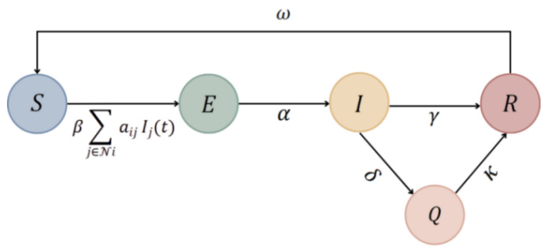
Based on mean-field theory and the network’s connectivity and transmission rules, we can derive differential equations for the average state of each node. The contagion mechanism is as follows: If an undistressed bank is adjacent to an infectious neighbor, it transitions from S to the exposed compartment ( E ) at rate β . The exposed state E indicates that a bank has been infected but that the risk has not yet manifested visibly or become transmissible to others. Exposed banks transition spontaneously to the infectious compartment I at rate α , regardless of whether they are adjacent to an infectious node. At this point, the bank exhibits overt risk characteristics and can transmit to its neighbors. Infectious banks may be isolated by regulators, moving from I to the quarantined compartment Q at rate δ . Quarantined banks recover and enter the immune class R at rate κ . Infectious banks that are not quarantined recover naturally into R at rate γ . Recovered banks lose immunity and return to the susceptible class S at rate ω . Combining these transitions, the time-evolution equations for a single node i can be written as:
d S i t d t = β j N i a i j S i t I j t + ω R i t d E i t d t = β j N i a i j S i t I j t α E i t d I i t d t = α E i t δ + γ I i t d Q i t d t = δ I i t κ Q i t d R i t d t = γ I i t + κ Q i t ω R i t
Here,   a i j is the adjacency matrix element, and N i represents the set of nodes connected to node i . If we adopt a probabilistic interpretation, S i t , E i t , I i t , Q i t , R i t are the probabilities that nod i is in the susceptible, exposed, infectious, quarantined, and recovered states, respectively.

3.3. Heterogeneous Mean-Field Approximation

Theorem 2
(Heterogeneous Mean-Field Approximation). Consider a scale-free network whose degree distribution satisfies
p k = N k N ,
with an average degree
k = k k p k ,
And the second moment
k 2 = k k 2 p k .
Assume that each node’s state depends only on its degree k , and that the probability of a neighbor being infectious follows a uniform-mixing approximation. Then the time evolution of the density of nodes of degree k in each compartment is given by
d S k d t = β k Θ t S k t + ω R k t d E k d t = β k Θ t S k t α E k t d I k d t = α E k t δ + γ I k t d Q k d t = δ I k t κ Q k t d R k d t = γ I k t + κ Q k t ω R k t
Here, S k t ,   E k t ,   I k t ,   Q k ( t )   and   R k ( t ) are the densities of susceptible, exposed, infectious, quarantined, and recovered nodes of degree k . β is the transmission rate, α is the exposed-to-infectious transition rate, δ is the quarantine rate, γ is the natural recovery rate, κ is the quarantine-recovery rate, and ω is the immunity-loss rate; Θ t is the probability that a randomly chosen neighbor is infectious, given by
Θ t = 1 k k k   P l I k t .
All higher-order neighbor–neighbor correlation terms have been replaced by the global quantity   Θ ( t )   , so that the system closes under the heterogeneous mean-field assumption. Model parameter values are summarized in Table 2.
By capturing the dynamic changes in the proportions of nodes in each compartment, this model characterizes the processes of risk transmission and recovery in the financial system. The contagion process among banks is illustrated in Figure 2.

3.4. Mathematical Analysis of the SEIQRS Model Under Heterogeneous Mean Fields

3.4.1. Basic Reproduction Number R 0 in HMF Form (Next-Generation Method)

Linearize around the disease-free equilibrium (DFE), where E k = I k = Q k = R k = 0, and S k = S k 0 . Apply the next-generation matrix approach in degree-class space. The new-infection operator from I k to E k has entries
F k k = β k S k 0 k P k k .
The remaining transition rates in the infection subsystem (for E and I variables) form diagonal blocks with rate α and δ + γ . Computing the next-generation matrix K = F V 1 yields a rank-one form
K k k = β δ + γ 1 k k S k 0 k P k .
A rank-one matrix u v T has a single nonzero eigenvalue equal to v T u ; therefore the spectral radius (the basic reproduction number) equals
R 0 = β δ + γ 1 k k k 2 S k 0 P ( k ) .
If the population is fully susceptible at baseline, S k 0 = 1, this simplifies to the familiar HMF result
R 0 = β δ + γ k 2 k .

3.4.2. Local Stability of the Disease-Free Equilibrium (DFE)

By the next-generation matrix theory [13], the disease-free equilibrium (DFE) is locally asymptotically stable when R 0 < 1 and unstable when R 0 > 1 . In the heterogeneous mean-field setting, this criterion takes the form given in (20): when the left-hand side of (20) is below one, infection-driven perturbations decay, whereas if it exceeds one, perturbations grow and a nontrivial endemic branch bifurcates from the DFE.
R 0 = β δ + γ 1 k k k 2 S k 0 P ( k ) < 1 ,
To keep the manuscript focused on the network-based characterization of R 0 and the policy simulations, we do not present closed-form expressions for endemic prevalences here. All steady states and their implications are instead obtained numerically in the simulation study (Section 3.5).

3.5. Numerical Simulation

For the initialization of the infection-propagation process, we assume that prior to a crisis, the majority of nodes are in the susceptible state while only a small fraction are infected. Following Hu Z. H. et al. [14] and the observation that long-term equilibria are largely determined by network structure rather than initial conditions, we set the initial node proportions in the SEIQRS model as S ( 0 ) = 0.80, E ( 0 ) =   0.05, I 0 = 0.05, R ( 0 ) = 0.10, representing susceptible, exposed, infectious, and recovered spots, respectively. The model parameters were fixed at β , γ , ω , α , δ , κ = [0.24, 0.10, 0.10, 0.20, 0.10, 0.18], which correspond to the transmission rate, natural recovery rate, immunity-loss rate, exposed-to-infectious transition rate, quarantine rate, and quarantine-recovery rate, respectively.
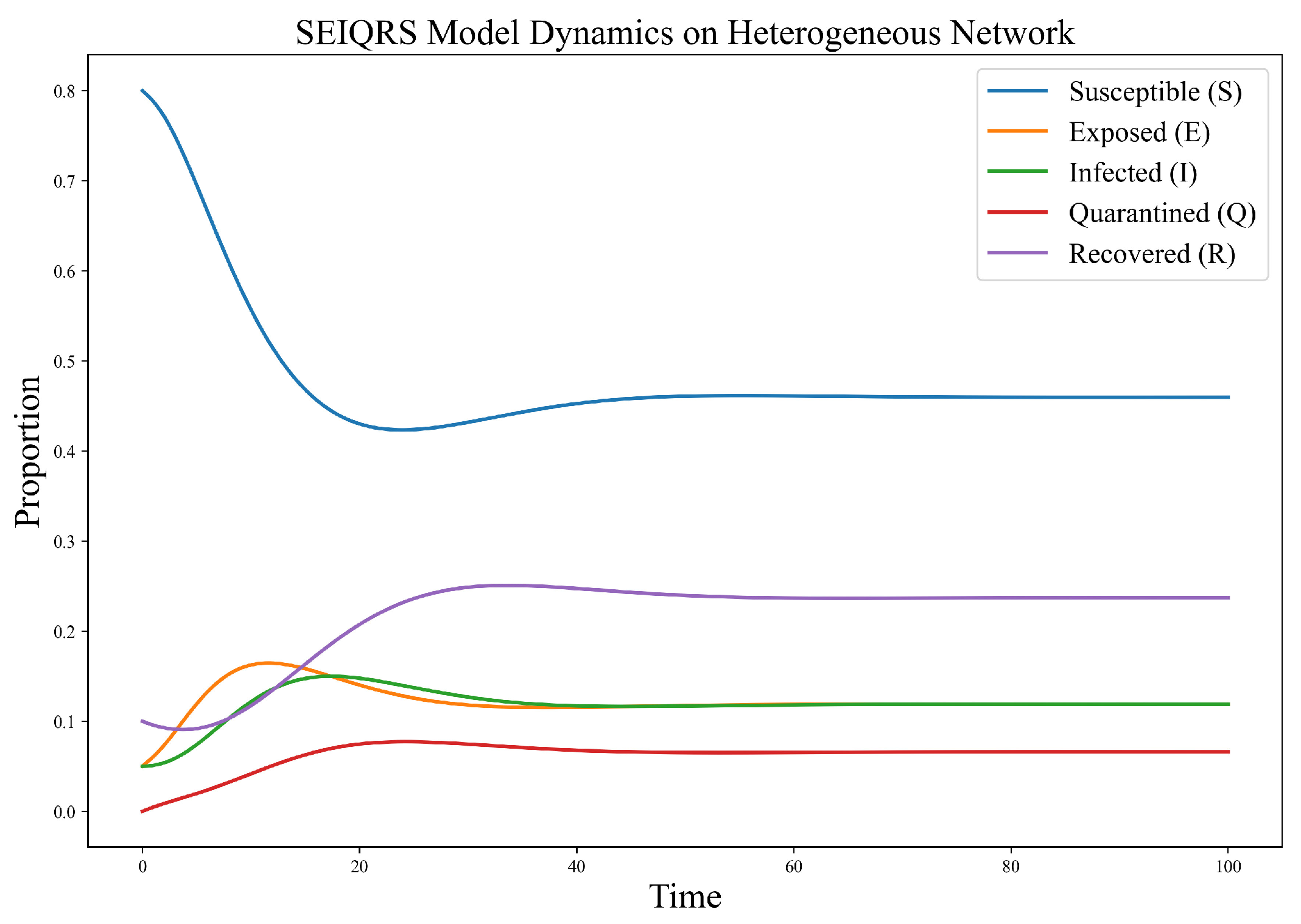
We then numerically integrate the system of state-evolution equations to simulate how risk spreads from infectious to susceptible nodes and to assess the influence of network parameters on contagion dynamics. Consistent with the theoretical analysis in Section 3.4, the disease-free equilibrium is stable when the basic reproduction number is below one, whereas an endemic equilibrium emerges once this threshold is exceeded. Although closed-form endemic solutions are not derived due to their algebraic complexity, their existence is guaranteed by the bifurcation result and is further corroborated by the numerical simulations. As shown in Figure 3, the proportions of all compartments converge to nontrivial steady values after transient fluctuations, confirming the presence of a stable endemic state in the heterogeneous network setting.
Starting from S ( t ) = 0.80, the susceptible fraction drops rapidly to approximately 0.42, then rebounds slightly, but ultimately stabilizes around 0.45 due to the ongoing interbank risk crisis. The delay between counterparty exposure and actual liquidity shortfalls creates a latent period: many banks enter the exposed state   ( E )   after the first wave of risk, but not all progress to infection, consistent with early-warning signals such as counterparty-risk monitoring and fluctuations in interbank pledge rates in the Chinese market. The peak in the infectious fraction   ( I )   indicates that, after the large core banks first lose stability, a cohort of mid-sized institutions also falls into distress. Quarantined banks   ( Q )   represent those temporarily isolated by regulators or subject to interbank funding freezes, effectively severing their funding chains and placing them under restructuring or special liquidity support. Banks that are isolated will return to R at a faster rate than the natural recovery rate, but they could still return to the “vulnerable” queue.

3.6. Sensitivity Analysis

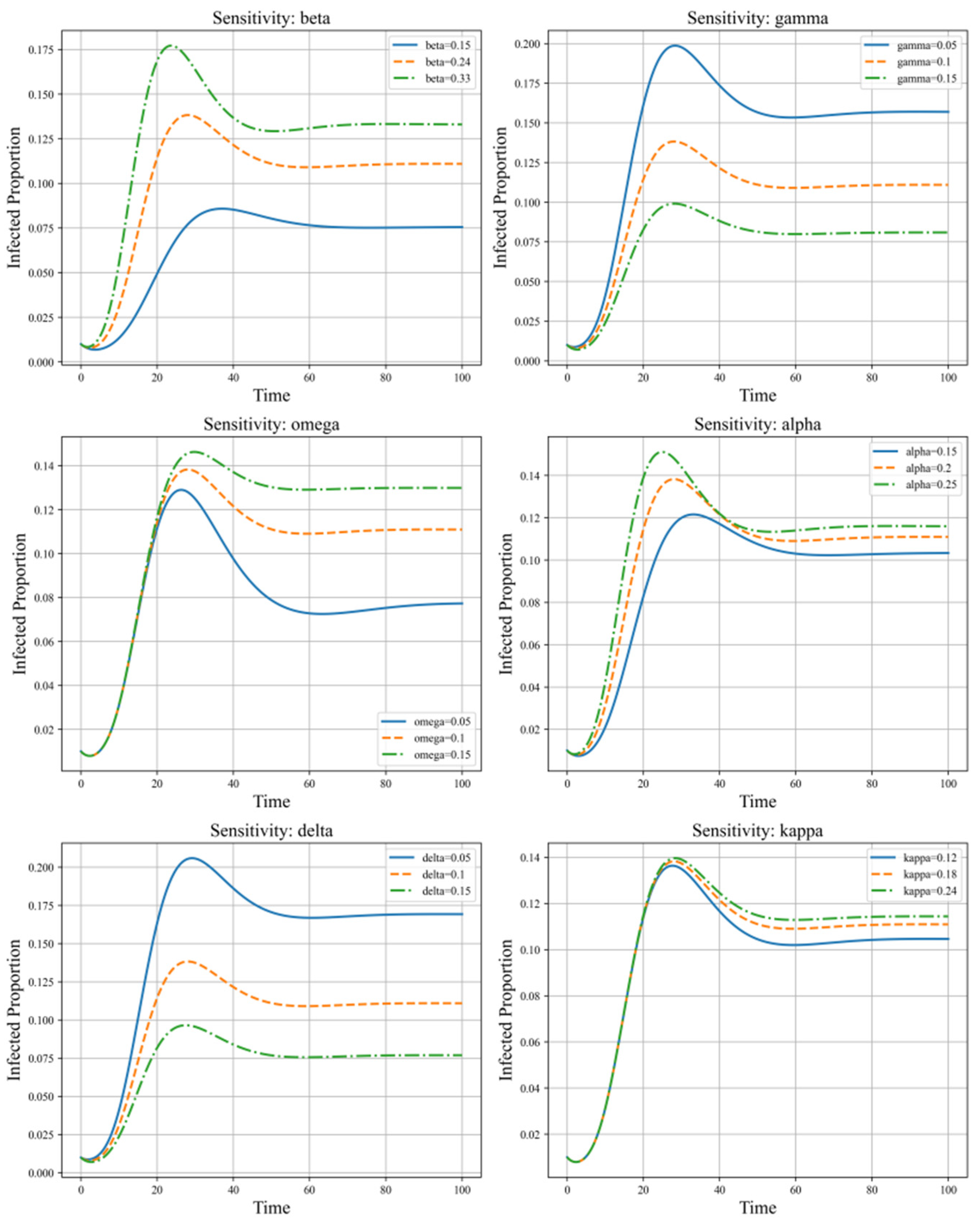
The sensitivity analysis in Figure 4 demonstrates that the transmission rate β , natural recovery rate γ , and quarantine rate δ have the strongest impact on the peak height and transmission speed of risk spread, corresponding to the three mechanisms of “acceleration-amplification”, “inhibition-accelerated decay”, and “quarantine-peak reduction.”
The exposed-to-infectious transition rate α determines the speed at which latent risks transform into overt risks and significantly affects the timing and height of the peak. The immunity-loss rate ω primarily influences the sustained infection levels in the tail of the risk transmission curve. In this model, the quarantine-recovery rate κ has the least sensitivity and can be considered a secondary regulatory parameter.
Therefore, in the design of prevention and control strategies, priority should be given to rapidly reducing the risk peak by reducing β and increasing γ and δ , while taking into account the control of immune loss and ensuring that the tail infection level is under control.

4. Simulation of Rescue Strategies

In Section 2, we constructed an empirical scale-free network of 36 listed Chinese banks. In this section, we generate a simulated scale-free network with the same node structure to evaluate crisis-time rescue strategies and derive policy recommendations for systemic-risk mitigation in the Chinese banking sector.

4.1. Assumptions

In a financial network, once contagion accelerates, rescue measures often become unavoidable. Although in the early phase of an outbreak, rescue actions typically do not directly alter the underlying transmission probabilities or immunity parameters, consistent with our model’s assumption of exogenous network parameters, intervention can nonetheless have pronounced short-term effects.
Specifically, by altering the distribution of banks across compartments, crisis-time bailouts can significantly reduce the peak infection fraction and shorten the crisis duration, even if they do not affect the long-run steady state. Accordingly, we adopt two evaluation metrics for bailout efficacy: the maximum fraction of infectious banks and the time at which this peak occurs. We fix the bailout “strength” at 20% of the total node count, that is, each rescue operation converts 20% of currently infectious banks into the immune compartment.

4.2. Parameters and Rescue-Strategy Design

For our network simulation, we initialize the compartmental proportions as follows: S ( 0 ) = 0.80, E ( 0 ) = 0.05, I 0 = 0.05, R ( 0 ) = 0.10. We then select a representative set of transmission and recovery parameters β , γ , ω , α , δ , κ = [0.24, 0.10, 0.10, 0.20, 0.10, 0.18] to benchmark the performance of different rescue strategies. All simulations are implemented in Python.
Based on the network’s topology, we compare three one-shot rescue strategies: the high-degree-first rescue strategy (priority is given to core nodes that have more connections with other nodes), the low-degree-first rescue strategy (priority is given to marginal nodes), and the balanced rescue strategy (uniform assistance is carried out without distinguishing the degree of nodes). By examining how each strategy influences the peak infection fraction and its timing, we assess their relative effectiveness in suppressing contagion under limited rescue resources.

4.3. The Impact of Rescue Timing on Strategy Effectiveness

In addition to selecting an appropriate rescue strategy, the timing of its implementation plays a critical role in determining its ultimate effectiveness. Identifying the optimal moment to intervene during a crisis, therefore, has important practical implications.

4.3.1. Impact of Rescue Timing on the Transmission Rate

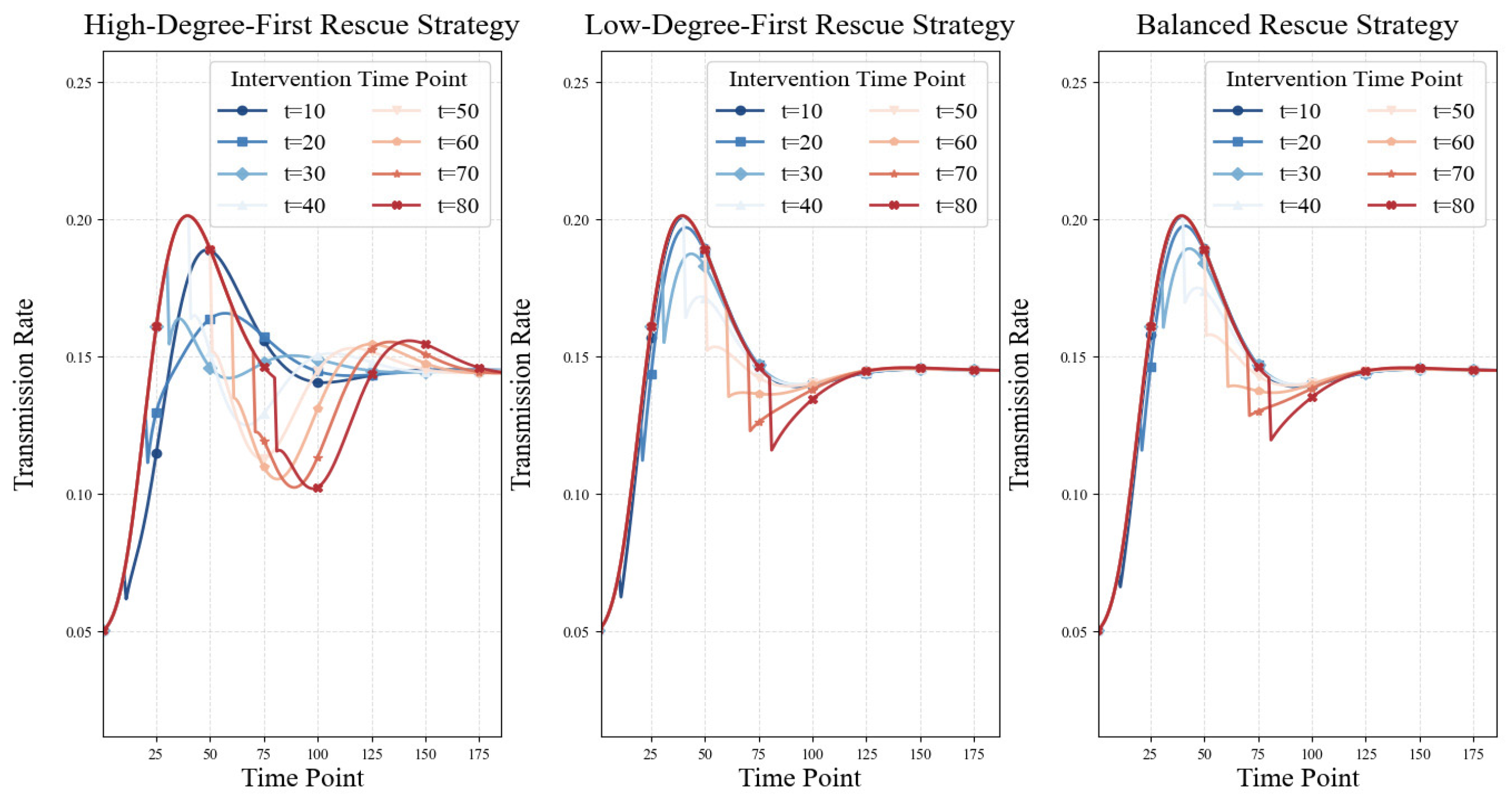
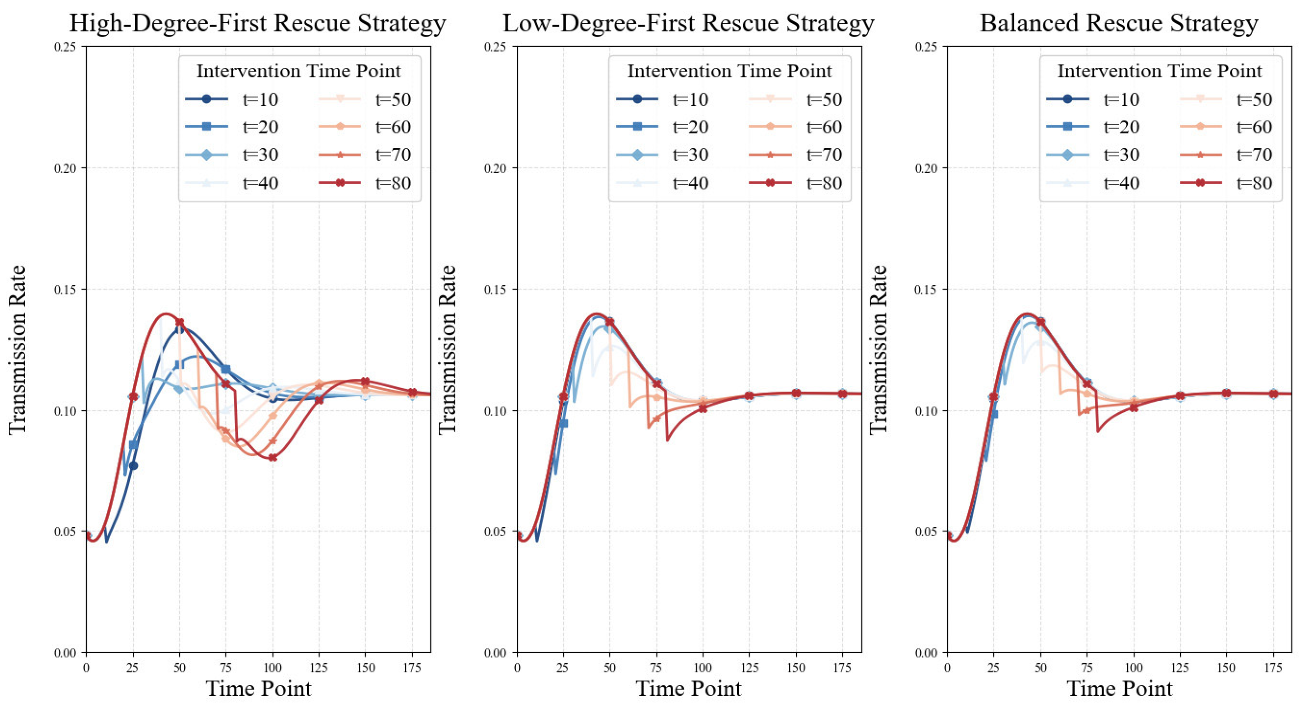
The overall proportion of distressed bank nodes   ( I ) , provides an intuitive measure of how deeply the crisis has penetrated the network and thus constitutes a key indicator of crisis evolution. To explore the effect of intervention timing, we perform a preliminary analysis by varying the time t , at which a fraction of infected nodes is “rescued” (moved from the distressed compartment back to the recovered compartments). Figure 5 shows, for each of eight equally spaced intervention times t = 10, 20, …, 80, the ensuing dynamics of I ( t ) under three different rescue-allocation strategies.
In the high-degree-first rescue strategy, the bank transmission rate after rescue at different specific times exhibits two major characteristics. First, the short-term effect is evident. After some banks receive assistance, the overall transmission rate in the banking network will continuously decline over a period of time, achieving a certain level of recovery. Second, there is still a noticeable “overshoot” phenomenon [14], which refers to the phenomenon where the transmission rate exceeds the long-term steady-state value.
Figure 5 above shows the temporal response of the network-wide infection proportion under three rescue-allocation strategies. The high-degree-first strategy effectively cuts transmission through major hubs and thus rapidly reduces the initial infection peak, but it can induce pronounced “overshoot” and subsequent rebounds when recovered nodes lose immunity or re-enter the susceptible pool. In the low-degree-first and balanced rescue strategies, the transmission rate often rebounds immediately after rescue because these strategies exert less direct control over highly connected infective banks, leaving the system vulnerable to re-seeding by banks closely linked to major crisis nodes; nonetheless, both strategies are more effective at mitigating the overshoot magnitude.
A sensitivity analysis reveals that increasing the quarantine rate preemptively weakens transmission chains, and delays in the exposed-to-infectious transition rate significantly alter the path of risk evolution. Raising the quarantine-recovery rate has only a modest impact on the infection peak, but by shortening each quarantine period, it frees up rescue resources and thus indirectly strengthens dynamic control. Accordingly, we modify the key parameters α , δ , κ =   [0.20, 0.10, 0.18] to α , δ , κ =   [0.15, 0.15, 0.23], and then re-evaluate the three rescue strategies. The results are plotted in Figure 6.
As shown in the figure, the transmission rates of the three rescue strategies have significantly decreased compared to the previous section, where only I node transfers to R nodes were performed. Meanwhile, the high-degree-first strategy still exhibits a clear short-term effect and also shows an “overshoot” phenomenon; the characteristics of the low-degree-first strategy and balanced rescue strategy remain consistent with the results from the previous section.

4.3.2. Impact of Rescue Timing on Strategy Effectiveness and the Optimal Rescue Time Point

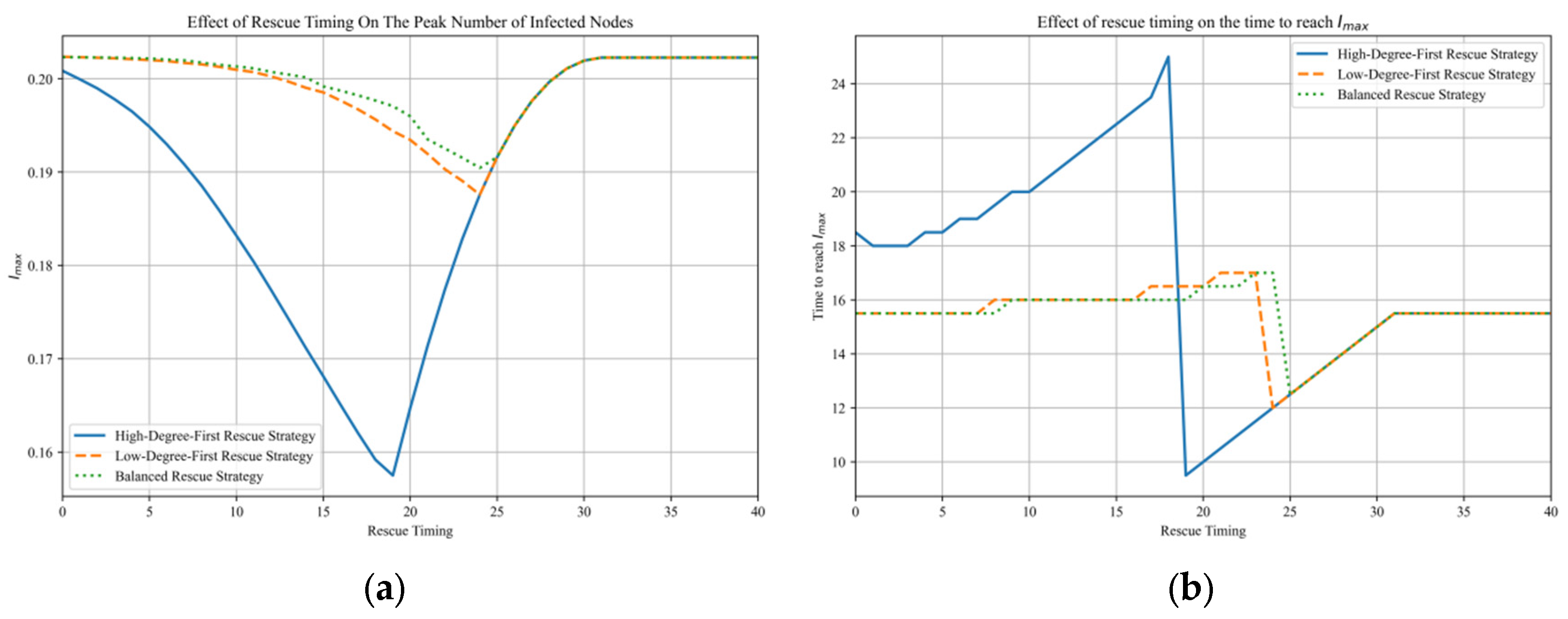
In this study, we select two key metrics to quantify the severity of contagion and thereby evaluate the effectiveness of rescue interventions: the maximum infection ratio   ( I m a x )   and the time at which this maximum infection ratio is reached   ( T m a x ) . The smaller the values of these two metrics, the less damage the contagion inflicts on the overall banking network, indicating a more effective strategy implementation.
According to Hu Zhihao et al. [14], there exists an optimal time point for implementing a rescue intervention during a single crisis episode. At this moment, the intervention yields the best outcome. This point is typically defined as the earliest time at which, once the rescue is applied, the total proportion of infected nodes in the network never exceeds the level observed at that moment. It is also referred to as the first non-worsening time point.
By simulating the contagion process under every possible rescue time point and recording the values of our metrics, we can assess the performance of three classes of strategies and determine the optimal timing for intervention. Figure 7 illustrates how these key metrics vary with the rescue time point under different strategies.
For the maximum transmission rate   ( I m a x ) , as the rescue time point is delayed, the peak infection ratio first decreases to a minimum, then increases steadily before eventually stabilizing. For the point at which the maximum transmission rate is reached   ( T m a x ) , as the rescue time is delayed, the time to reach the infection peak initially increases, reaches a local maximum, then sharply drops to a minimum, and subsequently rises gradually until it stabilizes.
Further comparative analysis shows that the high-degree-first rescue strategy performs best in our simulations, achieving a significant reduction in the infection peak. By prioritizing high-degree nodes early in the crisis, this strategy effectively reduces the number of infected nodes, thereby markedly decelerating the contagion across the network. However, this strategy is highly sensitive to the timing of intervention: if applied too early, it may prolong the time needed to reach the infection peak.
In contrast, the low-degree-first and balanced rescue strategies exhibit relatively poorer performance. Under the low-degree-first rescue strategy, resources are directed to peripheral nodes with low degrees, which fails to disrupt critical transmission pathways and does not substantially curb the spread. Nevertheless, when resources are scarce, this strategy can still delay infections among peripheral nodes and thus exert a mitigating effect on the contagion. The balanced rescue strategy, which allocates resources evenly, moderately lowers the peak infection ratio and results in a more gradual contagion spread throughout the network.

5. Conclusions

Our study, based on an SEIQRS contagion framework, uses numerical experiments to compare different rescue strategies, design a “Monitoring-Warning-Quarantine” crisis management architecture, and identify the optimal timing for interventions to maximize mitigation effects. The research finds that both the structural position of rescued institutions and the timing of interventions are critically important to the outcomes of systemic contagion. Therefore, a targeted policy design that combines topology-aware rescue prioritization with real-time monitoring can significantly enhance the resilience of the financial system.
Regarding rescue strategies, a “high-degree-first” approach is most effective at suppressing the infection peak when contagion spreads rapidly and early. While inferior on aggregate system metrics, a “low-degree-first” rescue strategy can be a valuable precision instrument for protecting socially or regionally important but less-connected institutions (e.g., rural credit unions). The “balanced allocation” strategy delivers moderate, robust damping across a wide range of scenarios, making it suitable when key nodes are indistinct or when political constraints require a broad distribution of support.
Furthermore, the proposed “Monitoring-Warning-Quarantine” framework, anchored on continuous, multi-dimensional monitoring and threshold-triggered interventions, enables regulators to act on emerging risks before they escalate. This approach shifts regulation from a reactive crisis response to a proactive, data-driven containment strategy, preventing the amplification of systemic risk by severing contagion channels at an early stage. The study also identifies a “sensitive time window” in which rescue measures yield the greatest marginal benefit, underscoring the decisive role of timing and providing a quantitative basis for shifting regulatory policy from ex-post bailouts to ex-ante prevention. Ultimately, these findings offer a quantitative basis for designing more resilient financial systems by embedding principles of network-aware prioritization and precise timing into macroprudential policy.
Looking ahead, our study opens up several important avenues for further exploration in the financial domain. First, to more accurately reflect reality, future research could investigate heterogeneous contagion rates. This could involve introducing degree-dependent parameters to differentiate the contagion speed between large, highly connected banks and small, less connected ones. This would allow for a more nuanced analysis of how different-sized institutions influence contagion dynamics.
Second, a significant direction for future research is to incorporate the impact of permanent institutional failures. While our current model treats “infection” as a reversible state of distress, in reality, some institutions may fail permanently. Future models could explore how permanent failures alter contagion dynamics and macroeconomic impacts, providing insights for more comprehensive crisis management strategies.

Author Contributions

Conceptualization, B.S. and Y.L.; Methodology, B.S. and Y.L.; Formal analysis, B.S. and Y.L.; Resources, B.S. and Y.L.; Writing—original draft, B.S. and Y.L.; Writing—review and editing, B.S. and Y.L.; Visualization, B.S. and Y.L.; Funding acquisition, B.S. All authors have read and agreed to the published version of the manuscript.

Funding

This work was supported by The Fundamental Research Funds for the Central Universities; Project of Research and Development Center for Mathematics Teaching in Colleges and Universities (CMC20240402); Education and Teaching Reform Fund of Central University of Finance and Economics (2024ZCJG09); Project of Talent Development Professional Committee of Chinese Society of Educational Development Strategy (24ZX05); Disciplinary Funding of Central University of Finance and Economics.

Data Availability Statement

Restrictions apply to the availability of these data. Data were obtained from CSMAR and are available from the authors at https://data.csmar.com/ (accessed on 20 August 2025) with the permission of CSMAR.

Conflicts of Interest

The authors declare no conflicts of interest.

References

  1. Allen, F.; Babus, A.; Carletti, E. Financial Connections and Systemic Risk; National Bureau of Economic Research: Cambridge, MA, USA, 2010. [Google Scholar]
  2. Hüser, A.C. Too interconnected to fail: A survey of the interbank networks literature. Netw. Theory Financ. 2015, 1, 1–50. [Google Scholar] [CrossRef]
  3. Kermack, W.O.; McKendrick, A.G. A contribution to the mathematical theory of epidemics. Proc. R. Soc. London. Ser. A Contain. Pap. A Math. Phys. Character 1927, 115, 700–721. [Google Scholar] [CrossRef]
  4. Teng, Y.; Ma, S.; Qian, Q.; Wang, G. SEIR-diffusion modeling and stability analysis of supply chain finance based on blockchain technology. Heliyon 2024, 10, e24981. [Google Scholar] [CrossRef] [PubMed]
  5. Ye, L.S. A Study of Risk Contagion in Selected Global Equity Markets Based on a Complex Network Contagion Model. Master’s Thesis, Fujian University of Technology, Fuzhou, China, 2023. [Google Scholar]
  6. Shi, X.Y.; Gao, H.L. SEIQR Infectious Disease Model with Media Effects and Age Structure. Appl. Math. 2025, 38, 435–445. [Google Scholar]
  7. Tian, Z.W.; Wang, L.; Liu, C. Information Dissemination Mechanism Analysis and Model Construction of Micro-blog Based on Complex Network. Inf. Sci. 2015, 33, 15–21. [Google Scholar]
  8. Tong, M.; He, Y. Systemic Risk and Liquidity Rescue in Complex Financial Networks: A Study Based on China’s Large-value Payment System. J. Financ. Res. 2012, 39, 20–33. [Google Scholar]
  9. Xu, T. Research on Contagion in Interbank Market and Control Strategies Based on the Integration of Complex Network and Multi-Agent. Ph.D. Thesis, Southeast University, Nanjing, China, 2017. [Google Scholar]
  10. Barabási, A.L.; Albert, R. Emergence of scaling in random networks. Science 1999, 286, 509–512. [Google Scholar] [CrossRef] [PubMed]
  11. Krapivsky, P.L.; Redner, S.; Leyvraz, F. Connectivity of growing random networks. Phys. Rev. Lett. 2000, 85, 4629. [Google Scholar] [CrossRef] [PubMed]
  12. Feng, W.F.; Mu, X.Y. Systemic Financial Risk Contagion in Bank Interbank Lending Based on Complex Network. Ningxia Soc. Sci. 2023, 4, 135–140. [Google Scholar]
  13. Van den Driessche, P.; Watmough, J. Reproduction numbers and sub-threshold endemic equilibria for compartmental models of disease transmission. Math. Biosci. 2002, 180, 29–48. [Google Scholar] [CrossRef] [PubMed]
  14. Hu, Z.H.; Li, X.H. Contagion and Bailout Strategy in Complex Financial Networks—SIRS Model on the Chinese Scale-free Financial Network. Financ. Trade Econ. 2017, 38, 101–114. [Google Scholar]
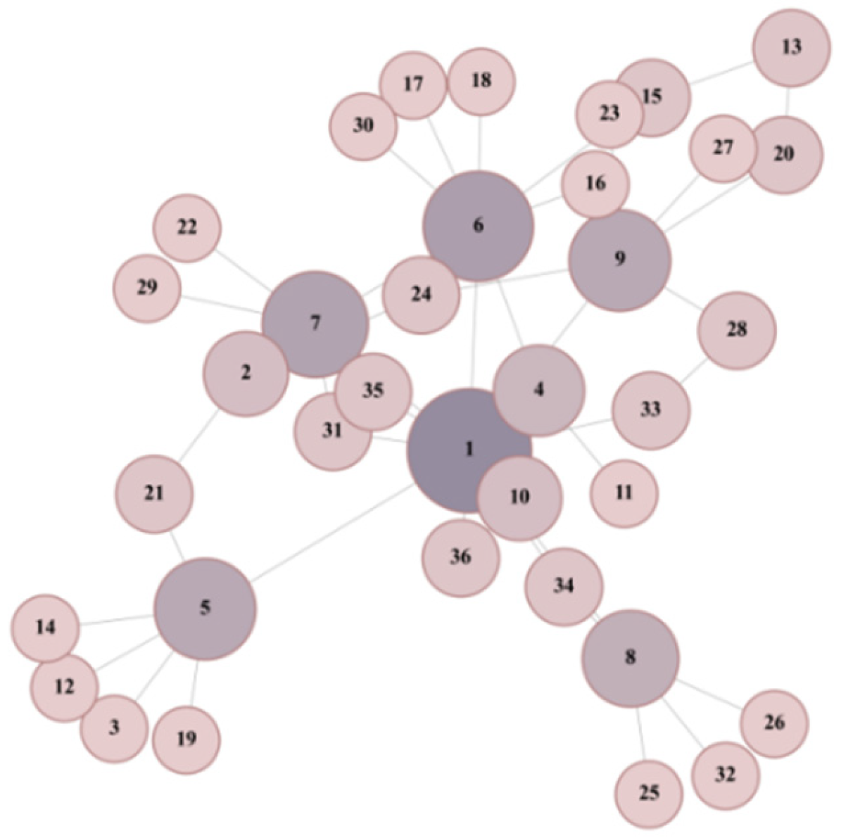
Figure 1. Interbank lending network topology (a dynamic directed graph constructed based on the matrix, where node size and color depth represent bank connectivity, and edges indicate actual lending relationships, illustrating the interbank lending activities among 36 banks. The numerical labels represent the bank sequence numbers sorted by scale of interaction).
Mathematics 13 03059 g001
Figure 2. Schematic diagram of the SEIQRS dynamic model (12).
Mathematics 13 03059 g002
Figure 3. The dynamic simulation results of the SEIQRS model on a heterogeneous network (in the plot, solid lines of different colors trace the time evolution of each compartment’s fraction: blue for susceptible (S), orange for exposed (E), green for infectious (I), red for quarantined (Q), and purple for recovered (R). The horizontal axis denotes time ( T i m e ) , and the vertical axis shows the node proportion ( P r o p o r t i o n ) . The ratio of the four types of nodes in the network is S ( 0 ) = 0.80, E ( 0 ) = 0.05, I 0 = 0.05, R ( 0 ) = 0.10; the parameters in the model are set to β , γ , ω , α , δ , κ = [0.24, 0.10, 0.10, 0.20, 0.10, 0.18]).
Mathematics 13 03059 g003
Figure 4. SEIQRS Model parameter sensitivity analysis (the subplots show the sensitivity of the transmission rate β , natural recovery rate γ , immunity-loss rate ω , exposed-to-infectious transition rate α , quarantine rate δ , and quarantine-recovery rate κ to different values. The colors and line styles in each subplot correspond to the different values of their respective parameters. The ratio of the four types of nodes in the network is S ( 0 ) = 0.80, E ( 0 ) = 0.05, I 0 =   0.05, R ( 0 ) = 0.10; the parameters in the sensitivity analysis are set separately to β = [0.15, 0.24, 0.33], γ = [0.05, 0.1, 0.15], ω = [0.05, 0.1, 0.15], α = [0.15, 0.2, 0.25], δ = [0.05, 0.1, 0.15], κ = [0.12, 0.18, 0.24]).
Mathematics 13 03059 g004
Figure 5. Dynamic response of the overall infection proportion under three strategies (the subplots show the dynamic effects of different rescue strategies on the proportion of distressed bank nodes in the network at eight specific time points when t = 10, 20, …, 80 under three strategies: high-degree-first strategy, low-degree-first strategy, and balanced rescue strategy).
Mathematics 13 03059 g005
Figure 6. The implementation effect of the three adjusted rescue strategies (the subplots, respectively, illustrate the dynamic impacts of implementing different rescue strategies on the overall proportion of distressed bank nodes in the network at eight specific time points t = 10, 20, …, 80, after reducing the exposed-to-infectious transition rate, increasing the quarantine rate, and improving the quarantine-recovery rate).
Mathematics 13 03059 g006
Figure 7. Variation of key metrics with rescue timing under different strategies. The subplots, respectively, illustrate the dynamic impacts of implementing different rescue strategies on the overall proportion of distressed bank nodes in the network at eight specific time points t = 10, 20, …, 80, after reducing the exposed-to-infectious transition rate, increasing the quarantine rate, and improving the quarantine-recovery rate: (a) description of the dynamic impacts of implementing different rescue strategies on the maximum infection ratio ( I m a x ) ; (b) description of the dynamic impacts of implementing different rescue strategies on the time at which this maximum infection ratio is reached ( T m a x ) .
Mathematics 13 03059 g007
Table 1. Selected Chinese banks (abbreviated bank names).
No.Bank NameNo.Bank NameNo.Bank Name
1ABC13SHBANK25CDCB
2ICBC14BOB26LZYH
3CCB15PSBC27CQBANK
4BOC16JSBANK28XMBANK
5CIB17CZBANK29ZZBANK
6BCM18NBBANK30QDCCB
7SPDB19HZCB31QDRCB
8CMBC20NJCB32QLBANK
9CMB21CQRCB33CSRCB
10CEB22SHRCB34RFRCB
11HXBANK23CSCB35XABANK
12SPABANK24BOSZ36SZRCB
Table 2. Model parameter settings.
SymbolDefinitionDescription
S SusceptibleA financial institution not yet hit by risk, but can be infected via network connections.
E ExposedA financial institution that has encountered risk but is not yet infectious; enters I after a latent period.
I InfectiousA financial institution currently experiencing risk and capable of transmitting it to others.
Q QuarantinedA financial institution isolated by regulators and temporarily unable to spread risk.
R RecoveredA financial institution that has recovered from risk but may lose immunity and become susceptible again over time.
β Transmission RateThe probability per contact that an infectious bank infects an undistressed bank.
α Exposed-to-infectious Transition RateThe rate at which exposed banks become infectious.
δ Quarantine RateThe rate at which infectious banks are isolated by regulators.
γ Natural Recovery RateThe rate at which infectious banks recover on their own without quarantine.
κ Quarantine-Recovery RateThe rate at which quarantined banks recover and become immune.
ω Immunity-Loss RateThe rate at which recovered banks lose immunity and return to the susceptible state.
Disclaimer/Publisher’s Note: The statements, opinions and data contained in all publications are solely those of the individual author(s) and contributor(s) and not of MDPI and/or the editor(s). MDPI and/or the editor(s) disclaim responsibility for any injury to people or property resulting from any ideas, methods, instructions or products referred to in the content.