General Decay Stability of Theta Approximations for Stochastic Delay Hopfield Neural Networks

Abstract

This paper investigates the general decay stability of the stochastic linear theta (SLT) method and the split-step theta (SST) method for stochastic delay Hopfield neural networks. The definition of general decay stability for numerical solutions is formulated. Sufficient conditions are derived to ensure the general decay stability of the SLT and SST methods, respectively. The key findings reveal that, under the derived sufficient conditions, both the SLT and SST methods can achieve general decay stability when $\theta \in \left[{\displaystyle \frac{1}{2}},1\right]$, while for the case of $\theta \in \left[0,{\displaystyle \frac{1}{2}}\right)$, the stability can also be guaranteed, which requires a stronger constraint on the step size. Finally, numerical examples are provided to demonstrate the effectiveness and validity of the theoretical results.

1. Introduction

Stochastic delay Hopfield neural networks (SDHNNs) have emerged as a cornerstone in the study of stochastic differential equations, offering powerful modeling frameworks for a diverse range of phenomena across multiple disciplines. Their applications span critical areas such as content-addressable memory systems, pattern recognition algorithms, and optimization theory, underscoring their practical significance in both theoretical research and real-world problem-solving. As a result, this class of stochastic delay differential equations has garnered substantial attention from scholars, with extensive explorations documented in the existing literature [1,2,3,4,5,6,7,8].

Stability analysis stands as a pivotal and compelling research direction for SDHNNs, as it directly governs the reliability and performance of these networks in practical applications. To address this, various stability criteria are established to investigate the stability of SDHNNs, such as [1,5]. Ref. [1] focused on the Euler numerical solution and established conclusions regarding exponential stability, while other works have explored different stability properties under varying conditions. In [2], the almost sure (a.s.) exponential stability of the Euler method and backward Euler method was researched. The mean square stability of split step Maruyama methods was considered in [3]. Ref. [7] studies a stochastic Hopfield neural network with multiple time-varying delays and Poisson jumps, proving analytical solutions’ stability and Euler method’s mean square stability. Ref. [8] explores delayed stochastic Hopfield neural network’s global behavior via random attractors, with conditions for their exponential attraction to stationary solutions. Recent studies on stability and stabilization of stochastic nonlinear systems, such as finite-time criteria [9], discrete-time stabilization [10], and fractional-order system methods [11,12], provide valuable insights for analyzing SDHNNs’ numerical stability.

The stability of numerical solutions in Hopfield neural networks, in general, holds immense significance. This is particularly true for SDHNNs, where the explicit analytical solutions are generally unavailable. This inherent lack of explicit analytical solutions elevates the importance of numerical solutions to an even greater degree, making them indispensable tools for conducting in-depth analysis and accurate simulation of SDHNNs. Among the existing numerical techniques, the theta family of methods has shown promise for solving stochastic differential equations, yet their stability behavior when applied to SDHNNs requires further scrutiny, such as [13,14,15,16,17,18,19,20]. Ref. [13] examined the exponential mean square stability of theta approximations for stochastic differential equations. Ref. [16] extended this by discussing the mean square exponential stability of theta methods for stochastic delay differential equations with neutral terms. Ref. [19] employed backward Euler approximation to investigate the general decay stability of nonlinear stochastic integro-differential equations, highlighting the growing interest in general decay stability as a more flexible and realistic stability criterion. Ref. [20] studied the mean square exponential stability of SST method and SLT method for SDHNNs.

The study of randomness impacts is of crucial importance in stability research ([21,22]). Specifically, Refs. [14,17,18,22] primarily discuss the mean square stability, almost sure stability, and asymptotically stability in probability, whereas [19] explore the more general concept of general decay stability. However, systematic studies on the general decay stability of key theta-type methods, specifically the SLT method and the SST method, for SDHNNs remain limited. To address this gap, we make the following contributions.

• Define general decay stability for the SLT and SST solutions of multi-delay SDHNNs, establishing a unified theoretical foundation;
• Derive sufficient conditions ensuring stability, explicitly linking parameters $\theta$ and step size h to decay rates;
• Reveal a critical phase transition: for $\theta \in [1/2,1]$, stability holds unconditionally, whereas $\theta \in [0,1/2)$ necessitates stricter step-size constraints.

Our work extends to two key aspects: (i) handling heterogeneous delays ${\tau }_j$, and (ii) establishing general decay stability (vs. mean-square exponential in [20]). This provides practitioners with explicit guidance for parameter selection in applications such as digital communication systems, where delays are integer multiples of a fixed step size.

The following is the organizational structure. In Section 2, we will introduce the notations, model and assumptions. Section 3 will investigate the general decay stability of the SST approximation. In Section 4, the general decay stability of the SLT approximation is studied. Finally, in Section 5, we provide a specific example to validate the conclusions.

2. Model and Assumptions

Let $(\mathsf{\Omega },\mathcal{F},{\left\{{\mathcal{F}}_t\right\}}_{t\ge 0},\mathbb{P})$ be a complete probability space with a filtration ${\left\{{\mathcal{F}}_t\right\}}_{t\ge 0}$. ${\left\{{\mathcal{F}}_t\right\}}_{t\ge 0}$ is increasing and right continuous, and ${\mathcal{F}}_0$ contains all $\mathbb{P}$-null sets. For $\tau >0$, $C([-\tau ,0],{\mathbb{R}}^n)$ represents the family of continuous functions from $[-\tau ,0]$ to ${\mathbb{R}}^n$ with norm ${\parallel \psi \parallel }_{\tau }={sup}_{-\tau \le \theta \le 0}|\psi (\theta )|$, in which $|·|$ represents the Euclidean norm in ${\mathbb{R}}^n$. $C_{{\mathcal{F}}_0}^b([-\tau ,0],{\mathbb{R}}^n)$ represents the family of all ${\mathcal{F}}_0$-measurable bounded $C([-\tau ,0],{\mathbb{R}}^n)$-valued random variables. $\{B(t)={(B_1(t),\dots ,B_n(t))}^T,t\ge 0\}$ is a standard Brownian motion of the n dimension defined in the probability space.

In this paper, we consider the SDHNNs as follows.

$$\left\{\begin{array}{cc}\hfill d{x}_i(t)=& [-c_i{x}_i(t)+\sum _{j=1}^n{a}_{ij}{f}_j(x_j(t))+\sum _{j=1}^n{b}_{ij}{g}_j(x_j(t-{\tau }_j))]dt+{\sigma }_i(x_i(t))d{B}_i(t),\hfill \\ \hfill x_i(t)=& {\xi }_i(t),-{\tau }_i\le t\le 0,\hfill \end{array}\right.$$

(1)

where $i=1,2,\dots ,n$, n is an integer that represents the number of neurons. $x_i(t)\in \mathbb{R}$ is the state variable of the ith neuron at time $t>0$, $f_j$, $g_j$ indicate the response of the jth neuron to input when the time is t and $t-{\tau }_j$, respectively. ${\tau }_j$ is a non-negative constant time delay in the signal transmission between neurons, which can take different values due to varying paths, embodying heterogeneous delays. ${\sigma }_i$ corresponds to the intensity of random disturbance on the ith neuron. $c_i$ is the rate of resetting its potential state when the unit encounters external stochastic disturbance. $a_{ij}$ and $b_{ij}$ weight the strength of the jth neuron on the ith unit. Let $\xi ={({\xi }_1(s),\dots ,{\xi }_n(s))}^T,-{\tau }_{\max }\le s\le 0$, in which ${\tau }_{\max }={max}_i{\tau }_i$ and ${\xi }_i(t)\in C_{{\mathcal{F}}_0}^b([-{\tau }_i,0],\mathbb{R})$ is an initial function when $t\in \left[-{\tau }_i,0\right]$.

Remark 1.

Clearly, time delays in the model represent delayed interactions between neurons. Compared with [1,14], the existence of multiple time delays complicates the reasoning process when deriving stability conclusions for numerical schemes. This paper shows that the time delays do not directly affect these stability criteria.

There exist many numerical schemes for stochastic ordinary differential equations. In [13], the SLT and SST methods are proposed for studying stochastic differential systems. In this paper, these two methods will be used to investigate SDHNNs.

Applying the SST method to Equation (1) yields

$$\left\{\begin{array}{cc}\hfill y_i^k=& x_i^k+\theta [-c_i{y}_i^k+\sum _{j=1}^n{a}_{ij}{f}_j(y_j^k)+\sum _{j=1}^n{b}_{ij}{g}_j(y_j^{k-m_j})]h,\hfill \\ \hfill x_i^{k+1}=& x_i^k+[-c_i{y}_i^k+\sum _{j=1}^n{a}_{ij}{f}_j(y_j^k)+\sum _{j=1}^n{b}_{ij}{g}_j(y_j^{k-m_j})]h+{\sigma }_i(y_i^k)\Delta B_i^k,\hfill \end{array}\right.$$

(2)

where $h>0$ is a step size satisfying ${\tau }_j=m_{j}h$ for some positive integer m. $t_k=kh$, $x_i^k$ is the SST approximate solution of $x_i(t_k)$. If $t_k\le 0$, $x_i^k=\xi (t_k),k=-m,-m+1,\dots ,-1,0$. The $\Delta B_i^k=B_i(t_{k+1})-B_i(t_k)$ is Brownian increment.

Applying the SLT method to Equation (1) yields

$$\begin{array}{cc}\hfill y_i^{k+1}=& y_i^k+\theta [-c_i{y}_i^{k+1}+\sum _{j=1}^n{a}_{ij}{f}_j(y_j^{k+1})+\sum _{j=1}^n{b}_{ij}{g}_j(y_j^{k-m_j+1})]h\hfill \\ & +(1-\theta )[-c_i{y}_i^k+\sum _{j=1}^n{a}_{ij}{f}_j\left(y_j^k\right)+\sum _{j=1}^n{b}_{ij}{g}_j(y_j^{k-m_j})]h+{\sigma }_i\left(y_i^k\right)\Delta B_i^k,\hfill \end{array}$$

(3)

where $y_i^k$ is the SLT approximate solution of $x_i(t_k)$.

Through derivation and calculation, it is interesting to note that the approximation $y_i$ in (3) is equal to the intermediate variable $y_i$ in (2). Thus, we can adopt the above unified notation in both the SST method and the SLT method.

Remark 2.

In SST and SLT methods, the requirements for ${\tau }_i$ may seem somewhat idealized. However, such requirements are easily satisfied or self-evident in practical applications. For example, one can impose that all ${\tau }_i$ are rational numbers. Alternatively, in digital communication systems, there exists an inherent communication step size, and all delays are integer multiples of this step size.

Remark 3.

When $\theta =0$, both the SST and SLT methods degenerate into the discrete Euler method in [1]. This indicates that the methods studied in our paper possess greater universality and generality, including the classical scheme as a special case.

SLT is actually the classical theta approximation, which is simpler and more widely used than the SST method. The goal of this paper is to investigate the general decay stability of numerical solutions (2) and (3). Firstly, the definition of decay function, namely $\varphi$-type function, is given as follows.

Definition 1.

If a function $\varphi (t):R\to (0,\infty )$ meets the following conditions:

(1) 

$\varphi (t)\in C(R;R^{+})$ is nondecreasing;

(2) 

$\varphi (0)=1,\varphi (\infty )=\infty$;

(3) 

$\varphi (s)\le \varphi (t)\varphi (s-t)$ for $s,t\ge 0$;

(4) 

$\phi =\underset{t\ge 0}{sup}[{\displaystyle \frac{{\varphi }^{\prime }(t)}{\varphi (t)}}]<\infty$.

then, $\varphi (t)$ is said to be ϕ-type function.

Remark 4.

It is straightforward to verify that commonly used functions such as $e^{\alpha t}$ (for exponential growth/decay) and ${(1+t)}^{\beta }$ (for polynomial growth/decay), where $\alpha ,\beta >0$, satisfy all four conditions outlined in the above definition. Hence, they are all ϕ-type functions.

We then present the definitions of general decay stability for numerical methods.

Definition 2.

For any positive step size h, a numerical solution $x_i^k,k\ge 0$ is generally decay stable if under any initial $\xi (kh)(k=-m,-m+1,\dots ,-1,0)$, and there exists a positive constant ε such that $x_i^k$ satisfies

$$\begin{array}{c}\hfill \underset{k\to \infty }{lim\; sup}{\displaystyle \frac{log|x_i^k|}{log\varphi (kh)}}<-\epsilon a.s..\end{array}$$

Remark 5.

According to condition (1–2) in Definition 1, we have $\varphi (t)\ge 1$ for all $t\ge 0$, which implies $ln(\varphi (t))\ge 0$. Mathematically, ε quantifies the convergence rate of the system state, governing the decay speed of the attenuation function—a larger ε implies faster convergence. In SDHNNs, it characterizes the decay rate of the energy function, reflecting how quickly the network stabilizes from its initial state. If the function ϕ in Definition 2 is replaced by $e^{\alpha t}$ or ${(1+t)}^{\beta }$, the general decay stability can be reduced to almost sure exponential stability and almost sure polynomial stability, respectively.

In order to obtain the stability of the numerical methods, we impose the following assumption.

Assumption 1.

$f_j(0)=g_j(0)=0$, ${\sigma }_i(0)=0$. $f_j$, $g_j$, ${\sigma }_i$ satisfy the global Lipschitz condition with Lipschitz constants ${\alpha }_j$, ${\beta }_j$, $L_i$, respectively.

Under this assumption, Equation (1) has a globally unique strong solution $x(t)=x(t,\xi )$ for $t\ge 0$, which is a measurable, sample-continuous and ${\mathcal{F}}_t$-adapted process with the initial function $\xi ={({\xi }_1,\dots ,{\xi }_n)}^T$.

Similar to [1], the following assumption is presented to ensure the general decay stability of the numerical scheme under the SST and SLT methods, which reflects the characteristic of weak interactions in the network and is a common type of stability condition widely applied in large-scale systems.

Assumption 2.

For $i=1,2,\dots ,n$,

$$-2c_i+2\sum _{j=1}^n|a_{ij}|{\alpha }_j+2\sum _{j=1}^n|b_{ij}|{\beta }_j+L_i^2<0.$$

(4)

To establish the stability theorem, the following result is required.

Lemma 1.

Under Assumption 1 and 2, the numerical scheme under the SST and SLT methods is well defined.

Proof of Lemma 1.

This lemma can be proven similarly to Lemma 3.2 in [20]. □

3. General Decay Stability of SST Approximation

To derive the key results of this section, we first introduce necessary notations to standardize the analysis, and present a critical lemma that serves as a foundational tool for theoretical development.

Suppose Assumption 1 and Assumption 2 hold, let $\overline{m}={max}_j\left\{m_j\right\}$. For $i=1,2,\dots ,n$, we define

$$\begin{array}{c}\hfill S_i(\epsilon ,h)={\tilde{P}}_i(h)+\sum _{j=1}^n{\tilde{Q}}_j(h)+{\varphi }^{\epsilon }\left(\overline{m}h\right)\sum _{j=1}^n{\tilde{R}}_j(h),\end{array}$$

and

$$\begin{array}{c}\hfill {\widehat{S}}_i(\epsilon ,h)={\widehat{P}}_i(h)+\sum _{j=1}^n{\widehat{Q}}_j(h)+{\varphi }^{\epsilon }\left(\overline{m}h\right)\sum _{j=1}^n{\widehat{R}}_j(h),\end{array}$$

where

$$\begin{array}{cc}\hfill P_i(h)=& -2c_{i}h+h\sum _{j=1}^n|a_{ij}|{\alpha }_j+h\sum _{j=1}^n|b_{ij}|{\beta }_j+\left(1-2\theta \right)c_i^2{h}^2+h{L}_i^2,\hfill \\ \hfill Q_j(h)=& h|a_{ij}|{\alpha }_j+\left(1-2\theta \right)h^2|a_{ij}|{\alpha }_j(\sum _{r=1}^n|a_{ir}|{\alpha }_r)+\left(1-2\theta \right)h^2|a_{ij}|{\alpha }_j\sum _{j=1}^n|b_{ij}|{\beta }_j,\hfill \\ \hfill R_j(h)=& h|b_{ij}|{\beta }_j+\left(1-2\theta \right)h^2|b_{ij}|{\beta }_j(\sum _{r=1}^n|b_{ir}|{\beta }_r)+\left(1-2\theta \right)h^2|a_{ij}|{\alpha }_j\sum _{j=1}^n|b_{ij}|{\beta }_j,\hfill \\ \hfill {\tilde{P}}_i(h)=& \left(1-{\varphi }^{-\epsilon }\left(h\right)\right)\left(1+\theta h\right)+\left(1-{\varphi }^{-\epsilon }\left(h\right)\right)\theta h\left(1+\theta h\right)c_i^2+P_i(h),\hfill \\ \hfill {\tilde{Q}}_j(h)=& 2\left(1-{\varphi }^{-\epsilon }\left(h\right)\right)\theta h\left(1+\theta h\right)|a_{ij}|{\alpha }_j(\sum _{r=1}^n|a_{ir}|{\alpha }_r)+Q_j(h),\hfill \\ \hfill {\tilde{R}}_j(h)=& 2\left(1-{\varphi }^{-\epsilon }\left(h\right)\right)\theta h\left(1+\theta h\right)|b_{ij}|{\beta }_j(\sum _{r=1}^n|b_{ir}|{\beta }_r)+R_j(h)\hfill \\ \hfill {\widehat{P}}_i(h)=& \left(1-{\varphi }^{-\epsilon }\left(h\right)\right)\left(1+\theta h\right)+\left(1-{\varphi }^{-\epsilon }\left(h\right)\right)\theta h\left(1+\theta h\right)c_i^2-2c_{i}h\hfill \\ \hfill & +h\sum _{j=1}^n|a_{ij}|{\alpha }_j+h\sum _{j=1}^n|b_{ij}|{\beta }_j+h{L}_i^2,\hfill \\ \hfill {\widehat{Q}}_j(h)=& 2\left(1-{\varphi }^{-\epsilon }\left(h\right)\right)\theta h\left(1+\theta h\right)|a_{ij}|{\alpha }_j(\sum _{r=1}^n|a_{ir}|{\alpha }_r)+h|a_{ij}|{\alpha }_j,\hfill \\ \hfill {\widehat{R}}_j(h)=& 2\left(1-{\varphi }^{-\epsilon }\left(h\right)\right)\theta h\left(1+\theta h\right)|b_{ij}|{\beta }_j(\sum _{r=1}^n|b_{ir}|{\beta }_r)+h|b_{ij}|{\beta }_j.\hfill \end{array}$$

If $\theta \in [0,{\displaystyle \frac{1}{2}})$, let $h^{\ast }(\theta )={min}_i(h_i(\theta ))$, in which $h_i={\displaystyle \frac{2c_i-2{\sum }_{j=1}^n|a_{ij}|{\alpha }_j-2{\sum }_{j=1}^n|b_{ij}|{\beta }_j-L_i^2}{(1-2\theta )(c_i^2+{\left({\sum }_{j=1}^n|a_{ij}|{\alpha }_j+{\sum }_{j=1}^n|b_{ij}|{\beta }_j\right)}^2)}}$.

To obtain the stability result for SST, the following lemma is given to discuss the solvability of two equations under different conditions satisfied by the parameter $\theta$.

Lemma 2.

Suppose Assumptions 1 and 2 hold, $i=1,2,\dots ,n$,

(1) 

For any $\theta \in [0,{\displaystyle \frac{1}{2}})$, if $h\in (0,h^{\ast })$, the equation $S_i(\epsilon ,h)=0$ with respect to the variable ε has a unique solution.

(2) 

For any $\theta \in [{\displaystyle \frac{1}{2}},1]$ and any $h>0$, the equation ${\widehat{S}}_i(\epsilon ,h)=0$ with respect to the variable ε has a unique solution.

Proof. 

(1) Fix $\theta \in [0,{\displaystyle \frac{1}{2}})$ and $h\in (0,h^{\ast })$; based on the definition of $S_i(\epsilon ,h)$, we get

$$\begin{array}{cc}\hfill S_i^{\prime }(\epsilon ,h){\mid }_{\epsilon }=& {\varphi }^{-\epsilon }\left(h\right)ln\varphi \left(h\right)\left(1+\theta h\right)[1+\theta h{c}_i^2+2\theta h\sum _{j=1}^n|a_{ij}|{\alpha }_j(\sum _{r=1}^n|a_{ir}|{\alpha }_r)]\hfill \\ \hfill & +2{\varphi }^{\epsilon }\left(m_{j}h\right)ln\varphi \left(m_{j}h\right)\left(1-{\varphi }^{-\epsilon }\left(h\right)\right)\theta h(1+\theta h)\sum _{j=1}^n|b_{ij}|{\beta }_j(\sum _{r=1}^n|b_{ir}|{\beta }_r)\hfill \\ \hfill & +2{\varphi }^{\epsilon }\left(m_{j}h\right){\varphi }^{-\epsilon }\left(h\right)ln\varphi \left(h\right)\theta h(1+\theta h)\sum _{j=1}^n|b_{ij}|{\beta }_j(\sum _{r=1}^n|b_{ir}|{\beta }_r)\hfill \\ \hfill & +{\varphi }^{\epsilon }\left(m_{j}h\right)ln\varphi \left(m_{j}h\right)[h\sum _{j=1}^n|b_{ij}|{\beta }_j+\left(1-2\theta \right)h^2\sum _{j=1}^n|b_{ij}|{\beta }_j(\sum _{r=1}^n|b_{ir}|{\beta }_r)]\hfill \\ \hfill & +{\varphi }^{\epsilon }\left(m_{j}h\right)ln\varphi \left(m_{j}h\right)(1-2\theta )h^2\sum _{j=1}^n|a_{ij}|{\alpha }_j\sum _{j=1}^n|b_{ij}|{\beta }_j\hfill \end{array}$$

$ln(\varphi (h))>0,ln(\varphi (m_{j}h))>0$, then we have $S_i^{\prime }>0$.

Additionally,

$$\begin{array}{cc}\hfill S_i(0,h)=& (1-2\theta )h^2[c_i^2+\sum _{j=1}^n|a_{ij}|{\alpha }_j·(\sum _{r=1}^n|a_{ir}|{\alpha }_r)+\sum _{j=1}^n|b_{ij}|{\beta }_j·(\sum _{r=1}^n|b_{ir}|{\beta }_r)\hfill \\ & +2\sum _{j=1}^n|a_{ij}|{\alpha }_j·\sum _{j=1}^n|b_{ij}|{\beta }_j]+h(-2c_i+2\sum _{j=1}^n|a_{ij}|{\alpha }_j+2\sum _{j=1}^n|b_{ij}|{\beta }_j+L_i^2).\hfill \end{array}$$

Because $h<h^{\ast },1-2\theta >0$, and Assumption 2 holds, we derive $S_i(0,h)<0$. Furthermore, it is straightforward to show that ${lim}_{\epsilon \to \infty }S\left(\epsilon ,h\right)=\infty$. Therefore, by the intermediate value theorem for continuous functions, the equation $S_i(\epsilon ,h)=0$ admits a unique solution.

(2) For the case $\theta \in [{\displaystyle \frac{1}{2}},1]$, the proof is completely similar and is provided in Appendix A.

The proof is completed. □

In light of the above lemma, for $\theta \in [0,{\displaystyle \frac{1}{2}})$, let ${\epsilon }_i^{\ast }(h)$ denote the unique solution to $S_i(\epsilon ,h)=0$, and define ${\epsilon }^{\ast }(h)={min}_{1\le i\le n}{\epsilon }_i^{\ast }(h)$, which will be shorted to ${\epsilon }^{\ast }$ below. Similarly, for $\theta \in [{\displaystyle \frac{1}{2}},1]$, let ${\widehat{\epsilon }}_i^{\ast }(h)$ denote the unique solution to ${\widehat{S}}_i(\epsilon ,h)=0$, and define ${\widehat{\epsilon }}^{\ast }(h)={min}_{1\le i\le n}{\widehat{\epsilon }}_i^{\ast }(h)$, which will be shorted to ${\widehat{\epsilon }}^{\ast }$ below.

We now present the following theorem to establish the general decay stability of the SST approximation (2).

Theorem 1.

Suppose Assumptions 1 and 2 hold.

(1) 

For any $\theta \in [0,{\displaystyle \frac{1}{2}})$, and $h\in (0,h^{\ast })$, the numerical solution ${\left\{x_i^k\right\}}_{k\ge 0}$ of the SST method (2) satisfies

$$\begin{array}{c}\hfill \underset{k\to \infty }{lim\; sup}{\displaystyle \frac{log|x_i^k|}{log\varphi (kh)}}<-{\displaystyle \frac{{\epsilon }^{\ast }}{2}},a.s.,i=1,\dots ,n,\end{array}$$

that is, the numerical solution of the SST method is generally decay stable.

(2) 

For any $\theta \in [{\displaystyle \frac{1}{2}},1]$, and $h>0$, the numerical solution ${\left\{x_i^k\right\}}_{k\ge 0}$ in SST method (2) satisfies

$$\begin{array}{c}\hfill \underset{k\to \infty }{lim\; sup}{\displaystyle \frac{log|x_i^k|}{log\varphi (kh)}}<-{\displaystyle \frac{{\widehat{\epsilon }}^{\ast }}{2}},a.s.,i=1,\dots ,n,\end{array}$$

that is, the numerical solution of the SST method is generally decay stable.

Proof. 

(1) For a fixed parameter $\theta \in [0,{\displaystyle \frac{1}{2}})$ and any time step h within the range $(0,h^{\ast })$. From the numerical scheme (2) of SST method, one can get

$$\begin{array}{cc}\hfill |x_i^{k+1}{|}^2=& |x_i^k{|}^2+{[-c_i{y}_i^k+\sum _{j=1}^n{a}_{ij}{f}_j(y_j^k)+\sum _{j=1}^n{b}_{ij}{g}_j(y_j^{k-m_j})]}^2{h}^2+{\sigma }_i^2(y_i^k){(\Delta B_i^k)}^2\hfill \\ \hfill & +2x_i^k[-c_i{y}_i^k+\sum _{j=1}^n{a}_{ij}{f}_j(y_j^k)+\sum _{j=1}^n{b}_{ij}{g}_j(y_j^{k-m_j})]h+2x_i^k{\sigma }_i(y_i^k)\Delta B_i^k\hfill \\ \hfill & +2h[-c_i{y}_i^k+\sum _{j=1}^n{a}_{ij}{f}_j(y_j^k)+\sum _{j=1}^n{b}_{ij}{g}_j(y_j^{k-m_j})]{\sigma }_i(y_i^k)\Delta B_i^k\hfill \\ \hfill =& |x_i^k{|}^2+{[-c_i{y}_i^k+\sum _{j=1}^n{a}_{ij}{f}_j(y_j^k)+\sum _{j=1}^n{b}_{ij}{g}_j(y_j^{k-m_j})]}^2{h}^2+h{\sigma }_i^2(y_i^k)\hfill \\ \hfill & +2x_i^k[-c_i{y}_i^k+\sum _{j=1}^n{a}_{ij}{f}_j(y_j^k)+\sum _{j=1}^n{b}_{ij}{g}_j(y_j^{k-m_j})]h+m_k,\hfill \end{array}$$

(5)

where

$$\begin{array}{cc}\hfill m_k=& {\sigma }_i^2(y_i^k)[{(\Delta B_i^k)}^2-h]+2x_i^k{\sigma }_i(y_i^k)\Delta B_i^k\hfill \\ & +2h[-c_i{y}_i^k+\sum _{j=1}^n{a}_{ij}{f}_j(y_j^k)+\sum _{j=1}^n{b}_{ij}{g}_j(y_j^{k-m_j})]{\sigma }_i(y_i^k)\Delta B_i^k.\hfill \end{array}$$

(6)

From (2), it is straightforward to derive that

$$\begin{array}{c}\hfill x_i^k=y_i^k-\theta [-c_i{y}_i^k+\sum _{j=1}^n{a}_{ij}{f}_j(y_j^k)+\sum _{j=1}^n{b}_{ij}{g}_j(y_j^{k-m_j})]h.\end{array}$$

(7)

Substituting Equation (7) into Equation (2), we obtain

$$\begin{array}{cc}\hfill |x_i^{k+1}{|}^2=& |x_i^k{|}^2+2y_i^k[-c_i{y}_i^k+\sum _{j=1}^n{a}_{ij}{f}_j(y_j^k)+\sum _{j=1}^n{b}_{ij}{g}_j(y_j^{k-m_j})]h\hfill \\ & +h{\sigma }_i^2(y_i^k)+(1-2\theta ){[-c_i{y}_i^k+\sum _{j=1}^n{a}_{ij}{f}_j(y_j^k)\sum _{j=1}^n{b}_{ij}{g}_j(y_j^{k-m_j})]}^2{h}^2+m_k.\hfill \end{array}$$

(8)

Together with Assumption 1, it leads to

$$\begin{array}{cc}\hfill |x_i^{k+1}{|}^2\le & |x_i^k{|}^2+2|y_i^k|[-c_i|y_i^k|+\sum _{j=1}^n|a_{ij}|{\alpha }_j|y_j^k|+\sum _{j=1}^n|b_{ij}|{\beta }_j|y_j^{k-m_j}|]h+h{L}_i^2{|y_i^k|}^2\hfill \\ \hfill & +\left(1-2\theta \right)[-c_i|y_i^k|+\sum _{j=1}^n|a_{ij}|{\alpha }_j|y_j^k|+\sum _{j=1}^n|b_{ij}|{\beta }_j|y_j^{k-m_j}{|]}^2{h}^2+m_k.\hfill \end{array}$$

(9)

By virtue of the inequality $2ab\left|x\right|\left|y\right|\le ab[{\left|x\right|}^2+{\left|y\right|}^2]$, we derive

$$\begin{array}{c}\hfill |x_i^{k+1}{|}^2\le |x_i^k{|}^2+P_i(h)|y_i^k{|}^2+\sum _{j=1}^n{Q}_j(h)|y_j^k{|}^2+\sum _{j=1}^n{R}_j(h){|y_j^{k-m_j}|}^2+m_k,\end{array}$$

Utilizing the properties of $\varphi$-type function, we can obtain

$$\begin{array}{cc}\hfill & {\varphi }^{{\epsilon }_i^{\ast }}\left(\left(k+1\right)h\right)|x_i^{k+1}{|}^2-{\varphi }^{{\epsilon }_i^{\ast }}\left(kh\right){|x_i^k|}^2\hfill \\ \hfill & \le {\varphi }^{{\epsilon }_i^{\ast }}\left(\left(k+1\right)h\right)\left(1-{\varphi }^{-{\epsilon }_i^{\ast }}\left(h\right)\right)|x_i^k{|}^2+{\varphi }^{{\epsilon }_i^{\ast }}\left(\left(k+1\right)h\right)[P_i(h)|y_i^k{|}^2+\sum _{j=1}^n{Q}_j(h){|y_j^k|}^2\hfill \\ \hfill & +\sum _{j=1}^n{R}_j(h)|y_j^{k-m_j}{|}^2]+{\varphi }^{{\epsilon }_i^{\ast }}\left(\left(k+1\right)h\right)m_k.\hfill \end{array}$$

(10)

Furthermore, Equation (7) yields

$$\begin{array}{cc}\hfill |x_i^k{|}^2=& |y_i^k{|}^2+{\theta }^2{h}^2[-c_i|y_i^k|+\sum _{j=1}^n|a_{ij}|{\alpha }_j|y_j^k|+\sum _{j=1}^n|b_{ij}|{\beta }_j|y_j^{k-m_j}{|]}^2-2\theta h|y_i^k|[-c_i|y_i^k|\hfill \\ & +\sum _{j=1}^n|a_{ij}|{\alpha }_j|y_j^k|+\sum _{j=1}^n|b_{ij}|{\beta }_j|y_j^{k-m_j}|]\hfill \\ \hfill \le & \left(1+\theta h\right)|y_i^k{|}^2+\theta h\left(1+\theta h\right)[-c_i|y_i^k|+\sum _{j=1}^n|a_{ij}|{\alpha }_j|y_j^k|+\sum _{j=1}^n|b_{ij}|{\beta }_j|y_j^{k-m_j}{|]}^2\hfill \\ \hfill \le & \left(1+\theta h\right)|y_i^k{|}^2+\theta h\left(1+\theta h\right)[c_i^2|y_i^k{|}^2+2\sum _{j=1}^n|a_{ij}|{\alpha }_j(\sum _{r=1}^n|a_{ir}|{\alpha }_r)|y_j^k{|}^2\hfill \\ & +2\sum _{j=1}^n|b_{ij}|{\beta }_j(\sum _{r=1}^n|b_{ir}|{\beta }_r)|y_j^{k-m_j}{|}^2].\hfill \end{array}$$

(11)

By substituting (11) into (10), one gets

$$\begin{array}{cc}\hfill & {\varphi }^{{\epsilon }_i^{\ast }}\left(\left(k+1\right)h\right)|x_i^{k+1}{|}^2-{\varphi }^{{\epsilon }_i^{\ast }}\left(kh\right){|x_i^k|}^2\hfill \\ \hfill & \le {\varphi }^{{\epsilon }_i^{\ast }}\left(\left(k+1\right)h\right){\tilde{P}}_i(h)|y_i^k{|}^2+{\varphi }^{{\epsilon }_i^{\ast }}\left(\left(k+1\right)h\right)\sum _{j=1}^n{\tilde{Q}}_j(h){|y_j^k|}^2\hfill \\ \hfill & +{\varphi }^{{\epsilon }_i^{\ast }}\left(\left(k+1\right)h\right)\sum _{j=1}^n{\tilde{R}}_j(h){|y_j^{k-m_j}|}^2+{\varphi }^{{\epsilon }_i^{\ast }}\left(\left(k+1\right)h\right)m_k.\hfill \end{array}$$

Through recursion, we can obtain

$$\begin{array}{cc}\hfill & {\varphi }^{{\epsilon }_i^{\ast }}\left(\left(k+1\right)h\right){|x_i^{k+1}|}^2\hfill \\ \hfill & \le |x_i^0{|}^2+\sum _{p=0}^k{\varphi }^{{\epsilon }_i^{\ast }}\left(\left(p+1\right)h\right){\tilde{P}}_i(h)|y_i^p{|}^2+\sum _{p=0}^k{\varphi }^{{\epsilon }_i^{\ast }}\left(\left(p+1\right)h\right)\sum _{j=1}^n{\tilde{Q}}_j(h){|y_j^p|}^2\hfill \\ \hfill & +\sum _{p=0}^k{\varphi }^{{\epsilon }_i^{\ast }}\left(\left(p+1\right)h\right)\sum _{j=1}^n{\tilde{R}}_j(h){|y_j^{p-m_j}|}^2+\sum _{p=0}^k{\varphi }^{{\epsilon }_i^{\ast }}\left(\left(p+1\right)h\right)m_p.\hfill \end{array}$$

(12)

According to

$$\begin{array}{cc}\hfill & \sum _{p=0}^k{\varphi }^{{\epsilon }_i^{\ast }}\left(\left(p+1\right)h\right)\sum _{j=1}^n{\tilde{R}}_j(h){|y_j^{p-m_j}|}^2\hfill \\ \hfill =& \sum _{j=1}^n{\tilde{R}}_j(h)\sum _{p=0}^k{\varphi }^{{\epsilon }_i^{\ast }}((p+1)h){|y_j^{p-m_j}|}^2\hfill \\ \hfill =& \sum _{j=1}^n{\tilde{R}}_j(h)\sum _{p=-m_j}^{k-m_j}{\varphi }^{{\epsilon }_i^{\ast }}((p+1+m_j)h){|y_j^p|}^2\hfill \\ \hfill \le & \sum _{j=1}^n{\tilde{R}}_j(h){\varphi }^{{\epsilon }_i^{\ast }}(\overline{m}h)\sum _{p=-\overline{m}}^k{\varphi }^{{\epsilon }_i^{\ast }}((p+1)h){|y_j^p|}^2\hfill \\ \hfill \le & \sum _{p=0}^k{\varphi }^{{\epsilon }_i^{\ast }}((p+1)h){\varphi }^{{\epsilon }_i^{\ast }}(\overline{m}h)\sum _{j=1}^n{\tilde{R}}_j(h)|y_j^p{|}^2+\sum _{p=-\overline{m}}^{-1}{\varphi }^{{\epsilon }_i^{\ast }}((p+1)h){\varphi }^{{\epsilon }_i^{\ast }}(\overline{m}h)\sum _{j=1}^n{\tilde{R}}_j(h){|y_j^p|}^2,\hfill \end{array}$$

then

$$\begin{array}{cc}\hfill & {\varphi }^{{\epsilon }_i^{\ast }}\left(\left(k+1\right)h\right){|x_i^{k+1}|}^2\hfill \\ \hfill & \le |x_i^0{|}^2+\sum _{p=-\overline{m}}^{-1}{\varphi }^{{\epsilon }_i^{\ast }}((p+1)h){\varphi }^{{\epsilon }_i^{\ast }}(\overline{m}h)\sum _{j=1}^n{\tilde{R}}_j(h){|y_j^p|}^2+\sum _{p=0}^k{\varphi }^{{\epsilon }_i^{\ast }}\left(\left(p+1\right)h\right)m_p\hfill \\ \hfill & +\sum _{p=0}^k{\varphi }^{{\epsilon }_i^{\ast }}((p+1)h)[{\tilde{P}}_i(h)+\sum _{j=1}^n{\tilde{Q}}_j(h)+{\varphi }^{{\epsilon }_i^{\ast }}(\overline{m}h)\sum _{j=1}^n{\tilde{R}}_j(h)]\underset{j}{max}|y_j^p{|}^2\hfill \\ \hfill & =A_i+B_i+M_k+\sum _{p=0}^k{\varphi }^{{\epsilon }_i^{\ast }}((p+1)h)S_i({\epsilon }_i^{\ast },h)\underset{j}{max}|y_j^p{|}^2,\hfill \end{array}$$

where

$$\begin{array}{cc}\hfill A_i& =|x_i{|}^2,\hfill \\ \hfill B_i& =\sum _{p=-m_j}^{-1}{\varphi }^{{\epsilon }_i^{\ast }}\left(m_{j}h\right){\varphi }^{\epsilon }\left(\left(p+1\right)h\right)\sum _{j=1}^n{\tilde{R}}_j(h){|y_j^p|}^2,\hfill \\ \hfill M_k& =\sum _{p=0}^k{\varphi }^{{\epsilon }_i^{\ast }}\left(\left(p+1\right)h\right)m_p.\hfill \end{array}$$

Clearly, $A_i$ is a non-negative ${\mathcal{F}}_0$-measurable random variable and $B_i$ is a non-negative random variable, with both being independent of the time variable k. Because ${\epsilon }_i^{\ast }$ is the solution of $S_i(\epsilon ,h)=0$, and ${\epsilon }^{\ast }=min{\epsilon }_i^{\ast }$, we can get

$$\begin{array}{c}\hfill {\varphi }^{{\epsilon }^{\ast }}\left(\left(k+1\right)h\right)|x_i^{k+1}{|}^2\le {\varphi }^{{\epsilon }_i^{\ast }}\left(\left(k+1\right)h\right){|x_i^{k+1}|}^2\le A_i+B_i+M_k.\end{array}$$

(13)

According to non-negative semi-martingale convergence theorem in [19], for finite random variable $\delta >0$, ${lim\; sup}_{k\to \infty }{\varphi }^{{\epsilon }^{\ast }}(kh){|x_i^k|}^2\le \delta$, which means

$$\begin{array}{c}\hfill \underset{k\to \infty }{lim\; sup}{\displaystyle \frac{log|x_i^k|}{log\varphi (kh)}}<-{\displaystyle \frac{{\epsilon }^{\ast }}{2}},i=1,2,\dots ,na.s..\end{array}$$

(14)

(2) The proof for the case $\theta \in [{\displaystyle \frac{1}{2}},1]$ is entirely analogous. It suffices to note that $\theta \in [0,{\displaystyle \frac{1}{2}})$ along with the simplifications of the coefficients $P_i(h),Q_j(h),R_j(h)$, and consequently ${\epsilon }^{\ast }$. The detailed derivation is omitted herein.

The proof of this theorem is completed. □

Remark 6.

It follows from the above theorem that, if $\theta \in [{\displaystyle \frac{1}{2}},1]$, the numerical solution of the SST method satisfies the general decay stability for any step size; meanwhile, if $\theta \in [0,{\displaystyle \frac{1}{2}})$, a necessary upper bound on the step size must exist to ensure such stability. This indicates that the closer the numerical simulation is to the fully implicit Euler interpolation, the more relaxed the conditions for guaranteeing the general decay stability become.

4. General Decay Stability of SLT Approximation

The following theorem establishes the general decay stability of the SLT approximation (3).

Theorem 2.

Suppose Assumptions 1 and 2 hold, then $h^{\ast },{\epsilon }^{\ast },{\widehat{\epsilon }}^{\ast }$ are defined identically to those in Theorem 1.

(1) 

For any $\theta \in [0,{\displaystyle \frac{1}{2}})$, and $h\in (0,h^{\ast })$, the numerical solution ${y_i^k}_{k\ge 0}$ of the SLT method satisfies

$$\begin{array}{c}\hfill \underset{k\to \infty }{lim\; sup}{\displaystyle \frac{log|y_i^k|}{log\varphi (kh)}}<-{\displaystyle \frac{{\epsilon }^{\ast }}{2}},i=1,2,\dots ,na.s.,\end{array}$$

that is, the numerical solution of the SLT method is generally decay stable.

(2) 

For any $\theta \in [{\displaystyle \frac{1}{2}},1]$, and $h>0$, the numerical solution ${y_i^k}_{k\ge 0}$ in SLT method (3) satisfies

$$\begin{array}{c}\hfill \underset{k\to \infty }{lim\; sup}{\displaystyle \frac{log|y_i^k|}{log\varphi (kh)}}<-{\displaystyle \frac{{\widehat{\epsilon }}^{\ast }}{2}},i=1,2,\dots ,na.s.,\end{array}$$

that is, the numerical solution of the SLT method is generally decay stable.

Proof. 

(1) From Equation (7), we can get

$$\begin{array}{cc}\hfill |x_i^k{|}^2=& |y_i^k{|}^2-2\theta h[-c_i{y}_i^k+\sum _{j=1}^n{a}_{ij}{f}_j(y_j^k)+b_{ij}{g}_j(y_j^{k-m_j})]y_i^k\hfill \\ & +{\theta }^2{h}^2{[-c_i{y}_i^k+\sum _{j=1}^n{a}_{ij}{f}_j(y_j^k)+\sum _{j=1}^n{b}_{ij}{g}_j(y_j^{k-m_j})]}^2\hfill \\ \hfill \ge & |y_i^k{|}^2-2\theta h[-c_i{y}_i^k+\sum _{j=1}^n{a}_{ij}{f}_j(y_j^k)+b_{ij}{g}_j(y_j^{k-m_j})]y_i^k.\hfill \end{array}$$

(15)

Based on Assumption 1, we have

$$\begin{array}{cc}\hfill & 2(-c_i{y}_i^k+\sum _{j=1}^n{a}_{ij}{f}_j(y_j^k)+b_{ij}{g}_j(y_j^{k-m_j}))y_i^k\hfill \\ \hfill \le & -2c_i|y_i^k{|}^2+\sum _{j=1}^n|a_{ij}|{\alpha }_j(|y_i^k{|}^2+|y_j^k{|}^2)+\sum _{j=1}^n|b_{ij}|{\beta }_j(|y_i^k{|}^2+|y_j^{k-m_j}{|}^2)\hfill \\ \hfill =& (-2c_i+\sum _{j=1}^n|a_{ij}|{\alpha }_j+\sum _{j=1}^n|b_{ij}|{\beta }_j)|y_i^k{|}^2+\sum _{j=1}^n|a_{ij}|{\alpha }_j|y_j^k{|}^2+\sum _{j=1}^n|b_{ij}|{\beta }_j{|y_j^{k-m_j}|}^2.\hfill \end{array}$$

(16)

Together with (15) and Assumption 2, one can estimate further that

$$\begin{array}{cc}\hfill |y_i^k{|}^2& \le |x_i^k{|}^2+2\theta h[-c_i{y}_i^k+\sum _{j=1}^n{a}_{ij}{f}_j(y_j^k)+b_{ij}{g}_j(y_j^{k-m_j})]y_i^k\hfill \\ \hfill & \le |x_i^k{|}^2+\theta h[-2c_i+2\sum _{j=1}^n{a}_{ij}{\alpha }_j+2\sum _{j=1}^n|b_{ij}|{\beta }_j]\underset{j}{max}\left\{|y_i^k|,|y_j^{k-m_j}|\right\}\hfill \\ \hfill & \le |x_i^k{|}^2.\hfill \end{array}$$

(17)

Along with the general decay stability of SST approximation in Theorem 1, it follows that

$$\begin{array}{c}\hfill \underset{k\to \infty }{lim\; sup}{\displaystyle \frac{log|y_i^k|}{log\varphi (kh)}}\le \underset{k\to \infty }{lim\; sup}{\displaystyle \frac{log|x_i^k|}{log\varphi (kh)}}<-{\displaystyle \frac{{\epsilon }^{\ast }}{2}}a.s.,\end{array}$$

for $k\ge 0$ and $i=1,2,\dots ,n$.

(2) The proof for the case $\theta \in [{\displaystyle \frac{1}{2}},1]$ is entirely analogous, and the detailed derivation is omitted herein.

The proof of this theorem is completed. □

5. Numerical Example

In this section, we will provide an example to validate the results we have obtained. Let $\{B(t),t\ge 0\}$ be a scalar Brownian motion. Consider the following two-dimensional stochastic delay Hopfield neural network on $t\ge 0$.

$$\begin{array}{cc}\hfill \left(\begin{array}{c}{x}_1(t)\hfill \\ x_2(t)\hfill \end{array}\right)=-C& \left(\begin{array}{c}{x}_1(t)\hfill \\ x_2(t)\hfill \end{array}\right)dt+A\left(\begin{array}{c}f\left(x_1(t)\right)\hfill \\ f\left(x_2(t)\right)\hfill \end{array}\right)dt\hfill \\ \hfill & +D\left(\begin{array}{c}g\left(x_1(t-1)\right)\hfill \\ g\left(x_2(t-2)\right)\hfill \end{array}\right)dt+\left(\begin{array}{c}{\sigma }_1{x}_1(t)\\ {\sigma }_2{x}_2(t)\end{array}\right)dB(t).\hfill \end{array}$$

(18)

The initial values are $x_1(t)=t+1,t\in \left[-1,0\right]$ and $x_2(t)=t+1,t\in \left[-2,0\right]$, respectively. Let $f\left(x\right)=sin\left(x\right)$, $g\left(x\right)=x$,

$$C=\left(\begin{array}{cc}20& 0\\ 0& 20\end{array}\right),A=\left(\begin{array}{cc}2& -4\\ -5& 3\end{array}\right),D=\left(\begin{array}{cc}-3& 1\\ 4& 2\end{array}\right),\sigma =\left(\begin{array}{c}1\\ -2\end{array}\right).$$

It can be easily calculated that ${\alpha }_j={\beta }_j=1,j=1,2$. $L_1=1,L_2=2$. Obviously, Assumption 1 is satisfied. Then, through computation,

$$\begin{array}{c}\hfill -2c_i+2\sum _{j=1}^n|a_{ij}|{\alpha }_j+2\sum _{j=1}^n|b_{ij}|{\beta }_j+L_i^2=-19,i=1,\end{array}$$

$$\begin{array}{c}\hfill -2c_i+2\sum _{j=1}^n|a_{ij}|{\alpha }_j+2\sum _{j=1}^n|b_{ij}|{\beta }_j+L_i^2=-8,i=2,\end{array}$$

and therefore, Assumption 2 is also satisfied. According to Theorem 1, the SST method for Equation (1) is generally decay stable for the case of $h<h^{\ast }$, in which

$$\begin{array}{c}\hfill h^{\ast }=\underset{i}{min}\left\{h_i\right\}={\displaystyle \frac{2c_i-2{\sum }_{j=1}^n|a_{ij}|{\alpha }_j-2{\sum }_{j=1}^n|b_{ij}|{\beta }_j-L_i^2}{(1-2\ast \theta )\left(c_i^2+{\left({\sum }_{j=1}^n|a_{ij}|{\alpha }_j+{\sum }_{j=1}^n|b_{ij}|{\beta }_j\right)}^2\right)}}<0.0224.\end{array}$$

Then, we provide a remark below to show the analysis of these results.

Remark 7.

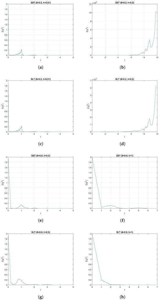
As demonstrated in Figure 1a–d, for $\theta =0.2$ (which belongs to $[0,{\displaystyle \frac{1}{2}})$), the SST and SLT methods exhibit distinct stability behaviors depending on the step size h. Specifically, when $h=0.01$ (which is less than the theoretically derived upper bound $h^{\ast }\approx 0.0224$), both methods converge to zero, satisfying the general decay stability as guaranteed by Theorems 1 and 2. In contrast, when $h=0.2$ (exceeding $h^{\ast }$), the numerical solutions fail to converge to zero in these examples.

For $\theta =0.9$ (belonging to $[{\displaystyle \frac{1}{2}},1]$), as shown in Figure 1e–h, both the SST and SLT methods remain stable even for larger step sizes ($h=0.2$ and $h=1$). This aligns with the theoretical results that stability is guaranteed for any positive step size in this θ interval, without additional constraints on h.

These numerical observations are consistent with our theoretical conclusions, highlighting that the stability of the SST and SLT methods is closely related to the choice of θ and, for $\theta \in [0,{\displaystyle \frac{1}{2}})$, the step size being bounded by $h^{\ast }$ is a sufficient condition to ensure general decay stability. It should be noted, however, that the derived condition $h\in (0,h^{\ast })$ is a sufficient condition rather than a necessary one. Thus, a step size slightly larger than $h^{\ast }$ does not necessarily imply instability; the guarantee of stability under such circumstances requires further analysis.

6. Conclusions

It is well-known that most stochastic delay Hopfield neural networks lack explicit analytical solutions, making it necessary to introduce numerical approximation methods such as the SST method to study their stochastic dynamics. In this paper, we consider both the SST and SLT methods, with the core objective of showing that both exhibit general decay stability under reasonable conditions. Our work further advances this field by addressing heterogeneous delays and establishing general decay stability, thereby providing explicit parameter selection guidance for applications like digital communication systems where delays are integer multiples of a fixed step.

References

- Li, R.; Pang, W.; Leung, P.K. Exponential stability of numerical solutions to stochastic delay hopfield neural networks. Neurocomputing 2010, 73, 920–926. [Google Scholar] [CrossRef]
- Liu, L.; Zhu, Q. Almost sure exponential stability of numerical solutions to stochastic delay Hopfield neural networks. Appl. Math. Comput. 2015, 266, 698–712. [Google Scholar] [CrossRef]
- Rathinasamy, A.; Narayanasamy, J. Mean square stability and almost sure exponential stability of two step Maruyama methods of stochastic delay Hopfield neural networks. Appl. Math. Comput. 2019, 348, 126–152. [Google Scholar] [CrossRef]
- Zhang, F.; Fei, C.; Fei, W. Stability of stochastic Hopfield neural networks driven by G-Brownian motion with time-varying and distributed delays. Neurocomputing 2023, 520, 320–330. [Google Scholar] [CrossRef]
- Tan, J.; Tan, Y.; Guo, Y.; Feng, J. Almost sure exponential stability of numerical solutions for stochastic delay Hopfield neural networks with jumps. Phys. Stat. Mech. Its Appl. 2020, 545, 123782. [Google Scholar] [CrossRef]
- Feng, L.; Cao, J.; Liu, L. Stability analysis in a class of Markov switched stochastic Hopfield neural networks. Neural Process. Lett. 2019, 50, 413–430. [Google Scholar] [CrossRef]
- Xu, H.; Luo, H.; Fan, X.Q. Stability of stochastic delay Hopfield neural network with Poisson jumps. Chaos Solitons Fractals 2024, 187, 115404. [Google Scholar] [CrossRef]
- Hu, W.; Zhu, Q.; Kloeden, P.E.; Duan, Y. Random attractors of a stochastic Hopfield neural network model with delays. Qual. Theory Dyn. Syst. 2024, 23, 222. [Google Scholar] [CrossRef]
- Cheng, M.; Zhao, J.; Xie, X.; Sun, Z. A novel finite-time stability criteria and controller design for nonlinear impulsive systems. Appl. Math. Comput. 2024, 479, 128876. [Google Scholar] [CrossRef]
- Zhang, T.; Xu, S.; Zhang, W. New approach to feedback stabilization of linear discrete time-Varying stochastic systems. IEEE Trans. Auto. Contr. 2025, 70, 2004–2011. [Google Scholar] [CrossRef]
- Rguigui, H.; Elghribi, M. Separation principle for Caputo-Hadamard fractional-order fuzzy systems. Asian J. Control 2025. [Google Scholar] [CrossRef]
- Rguigui, H.; Elghribi, M. Practical stabilization for a class of tempered fractional-order nonlinear fuzzy systems. Asian J. Control 2025, 1–7. [Google Scholar] [CrossRef]
- Huang, C. Exponential mean square stability of numerical methods for systems of stochastic differential equations. J. Comput. Appl. Math. 2012, 236, 4016–4026. [Google Scholar] [CrossRef]
- Huang, C. Mean square stability and dissipativity of two classes of theta methods for systems of stochastic delay differential equations. J. Comput. Appl. Math. 2014, 259, 77–86. [Google Scholar] [CrossRef]
- Mao, X. Convergence rates of the truncated Euler–Maruyama method for stochastic differential equations. J. Comput. Appl. Math. 2016, 296, 362–375. [Google Scholar] [CrossRef]
- Zong, X.; Wu, F.; Huan, C.G. Exponential mean square stability of the theta approximations for neutral stochastic differential delay equations. J. Comput. Appl. Math. 2015, 286, 172–185. [Google Scholar] [CrossRef]
- Liu, L.; Zhu, Q. Mean square stability of two classes of theta method for neutral stochastic differential delay equations. J. Comput. Appl. Math. 2016, 305, 55–67. [Google Scholar] [CrossRef]
- Li, M.; Deng, F. Almost sure stability with general decay rate of neutral stochastic delayed hybrid systems with Lévy noise. Nonlinear Anal. Hybrid Syst. 2017, 24, 171–185. [Google Scholar] [CrossRef]
- Liu, L.; Deng, F.; Qu, B.; Fang, J. General decay stability of backward Euler–Maruyama method for nonlinear stochastic integro-differential equations. Appl. Math. Lett. 2023, 135, 108406. [Google Scholar] [CrossRef]
- Liu, L.; Deng, F.; Zhu, Q. Mean square stability of two classes of theta methods for numerical computation and simulation of delayed stochastic Hopfield neural networks. J. Comput. Appl. Math. 2018, 343, 428–477. [Google Scholar] [CrossRef]
- Zhao, J.; Yuan, Y.; Sun, Z.; Xie, X. Applications to the dynamics of the suspension system of fast finite time stability in probability of p-norm stochastic nonlinear systems. Appl. Math. Comput. 2023, 457, 128221. [Google Scholar] [CrossRef]
- Cao, Y.; Zhao, J.; Sun, Z. State feedback stabilization problem of stochastic high-order and low-order nonlinear systems with time-delay. AIMS Math. 2023, 8, 3185–3203. [Google Scholar] [CrossRef]
Disclaimer/Publisher’s Note: The statements, opinions and data contained in all publications are solely those of the individual author(s) and contributor(s) and not of MDPI and/or the editor(s). MDPI and/or the editor(s) disclaim responsibility for any injury to people or property resulting from any ideas, methods, instructions or products referred to in the content. |
© 2025 by the authors. Licensee MDPI, Basel, Switzerland. This article is an open access article distributed under the terms and conditions of the Creative Commons Attribution (CC BY) license (https://creativecommons.org/licenses/by/4.0/).