Article

A New Proximal Iteratively Reweighted Nuclear Norm Method for Nonconvex Nonsmooth Optimization Problems

1
School of Mathematical Sciences, Nanjing Normal University of Special Education, Nanjing 210038, China
2
School of Microelectronics and Data Science, Anhui University of Technology, Ma’anshan 243032, China
3
School of Mathematics and Physics, Suqian University, Suqian 223800, China
4
Key Laboratory of Numerical Simulation for Large Scale Complex Systems, Ministry of Education, Nanjing 210023, China
5
School of Artificial Intelligence, Nanjing Normal University of Special Education, Nanjing 210038, China
*
Author to whom correspondence should be addressed.
Mathematics 2025, 13(16), 2630; https://doi.org/10.3390/math13162630
Submission received: 9 July 2025 / Revised: 13 August 2025 / Accepted: 13 August 2025 / Published: 16 August 2025
(This article belongs to the Special Issue Decision Making and Optimization Under Uncertainty)

Abstract

This paper proposes a new proximal iteratively reweighted nuclear norm method for a class of nonconvex and nonsmooth optimization problems. The primary contribution of this work is the incorporation of line search technique based on dimensionality reduction and extrapolation. This strategy overcomes parameter constraints by enabling adaptive dynamic adjustment of the extrapolation/proximal parameters (αk, βk, μk). Under the Kurdyka–Łojasiewicz framework for nonconvex and nonsmooth optimization, we prove the global convergence and linear convergence rate of the proposed algorithm. Additionally, through numerical experiments using synthetic and real data in matrix completion problems, we validate the superior performance of the proposed method over well-known methods.

1. Introduction

1.1. Problem Description

This work addresses a nonconvex and nonsmooth optimization problem within the real matrix space R m × n ( m n )
min X Ψ ( X ) : = f ( X ) + i = 1 m g ( σ i ( X ) ) ,
where σ i ( X ) denotes the i-th singular value of X, f is differentiable and the gradient is Lipschitz continuous with constant L f , g is differentiable concave and the gradient is Lipschitz continuous with constant L g and g ( t ) > 0 for any t [ 0 , + ) .
It is easy to see that i = 1 m g ( σ i ( X ) ) is nonconvex and nonsmooth due to the nonsmoothness of σ i ( X ) and the concavity of g. Thus, the overall function Ψ is nonconvex and nonsmooth even though f is differentiable (may be nonconvex). Note the generality of problem (1), it has a wide applications, such as image processing [1], machine learning [2] and multiple category classification [3]. To illustrate this point, consider the well-known image recovery problem. In such a scenario, f ( X ) = 1 2 A ( X ) b 2 (A is a linear operator and b is a vector or matrix) generally represents the quadratic loss function, which is used to measure recovery performance. Consequently, f is always differentiable. On the other hand, i = 1 m g ( σ i ( X ) ) is a nonconvex regularized term that is employed to obtain a low rank solution. Some common nonconvex regularized terms, including L p , Log, ETP, Geman and Laplace can be found in [1,4]. The validity of the assumption of g can be verified through the nonnegativity of its second order derivatives and the median theorem.

1.2. Related Work

It is precisely because of the popularity and scope of problem (1) that there is a lot of related work, as can be seen in [5,6,7,8,9,10,11,12,13]. One of the more competitive methods is the well-known General Iterative Shrinkage and Thresholding (GIST) algorithm [14,15]. Applying the GIST algorithm to solve (1) needs to compute the proximal operator of a DC function i = 1 m g ( σ i ( X ) ) . Unfortunately, this assumption of i = 1 m g ( σ i ( X ) ) is less likely to be satisfied, since the DC decomposition of i = 1 m g ( σ i ( X ) ) is not known in general. Thus, based on the key fact that nonnegativity and monotone decrease of g , Lu et al. [4] proposed Proximal Iteratively Reweighed Nuclear Norm algorithm (PIRNN). Sun et al. [16] refined the related convergence conclusions. Later, Ge et al. [1] gave the PIRNN with a more general Extrapolation (PIRNNE) and proved the convergence under the same assumptions. The concrete iterative scheme can be read as
{ (2) Y k : = X k + α k X k X k 1 (3) Z k : = X k + β k X k X k 1 (4) X k + 1 : = prox i = 1 m μ k w i k σ i ( X ) Y k μ k f Z k
where α k [ 0 , 1 ) , β k [ 0 , 1 ] are the extrapolation stepsizes, { μ k } is a nondecreasing parameter sequence, ω i k : = g ( σ i ( X k ) ) and for any Y R m × n ,
prox i = 1 m μ k w i k σ i ( X ) ( Y ) : = arg min X i = 1 m w i k σ i ( X ) + 1 2 μ k X Y F 2 .
(4) has a closed-form solution if 0 w 1 k w 2 k w m k . In other words, for any Y R m × n , one has U S ( Λ ) V prox i m μ w i k σ i ( X ) ( Y ) , where U Λ V is the SVD of Y, S ( Λ ) = diag { ( Λ i , i μ k w i k ) + } 1 i m with ( a ) + = max { a , 0 } for any a R .
Meanwhile, Phan et al. [17] devised an acceleration framework utilizing the partial singular value decomposition of reduced-dimensional matrices rather than full matrices, conditioned upon parameter specifications with α k = 0 , β k = k k + 3 and μ k = μ . Xu et al. [18] integrated rank estimation via enhanced Gerschgorin disk analysis with learnable submatrix recovery, demonstrating state-of-the-art performance. Separately, Wen et al. [19] formulated an alternative accelerated matrix completion methodology employing continuation protocols and randomized truncated SVD, parameterized by α k = β k = 0 and μ k + 1 = max { η μ k , μ min } , η < 1 . Generalized framework [20] leveraged ADMM for nonconvex nonsmooth low-rank recovery with rigorous convergence guarantees. Some recent methods also combine other regularization techniques. Alternative regularization strategies included an image reconstruction factorization model using a total variation regularizer [21], a truncated error model using the difference between the nuclear norm and Frobenius norm for impulse noise processing [22], and an accelerated iterative reweighted nuclear norm method combined with active manifold identification [23]. This paper focuses on the efficient computation of (5) based on PIRNNE. To the best of our knowledge, suitable parameter selection makes these algorithms have good numerical performance. The most famous optimal parameter choice is the Nesterov’s acceleration, such as FISTA [24] and APG [25]. The optimal choice involving the inertial and proximal parameters of PIRNNE for the nonconvex nonsmooth problems considered in this paper are not explicit, which makes the algorithm unable to maintain its advantage. Whether there is an adaptive parameter selection is our concern.

1.3. Our Contribution

Fortunately, the line search strategy is widely used for nonconvex vector optimization to overcome restrictions on the involved parameters [26,27,28,29,30,31]. This strategy allows the parameters to be chosen initially with some aggressive values that are not below a specific threshold, and then updates adaptively parameters at each iteration according to the line search criterion, which can improve the numerical performance in implementation. A natural approach is to incorporate the line search strategy to the PIRNNE by updating the parameters α k , β k and μ k . adaptively. Therefore, the main contributions of this paper are as follows:
  • We propose a Proximal Iteratively Reweighted Nuclear Norm algorithm with Extrapolation and Line Search, denoted by PIRNNE-LS. This framework integrates line search with extrapolation and dimensionality reduction, circumventing parametric limitations. Parameters withinthe proposed method initialize aggressively above defined thresholds then undergo criterion-driven adaptive recalibration per iteration.
  • We prove the subsequential convergence that each generated sequence converges to a stationary point of the considered problem. Especially, when the line search is monotone, we further establish its global convergence and linear convergence rate under the Kurdyka–Łojasiewicz framework.
  • We conduct some experiments to evaluate the performance of the proposed method for solving the matrix completion problem. Some numerical results are reported the effectiveness and superiority of our proposed method.
The remainder of this paper is organized as follows. Section 2 provides the preliminaries needed for the theoretical analysis in the subsequent sections. Section 3 details PIRNNE-LS for the specified problem. Section 4 analyzes the subsequential convergence. Specifically, we discuss the global convergence and linear convergence rate under the Kurdyka–Łojasiewicz framework in the case of monotone line search. Section 5 reports numerical results on synthetic and empirical datasets. Concluding conclusions appear in Section 6.

2. Preliminaries

In this section, we recall some definitions and properties which will be used in the analysis.

2.1. Basic Concepts in Variational and Convex Analysis

For an extended-real-valued function J : = R n ( , ] , its domain is defined by dom ( J ) : = { x R n : J ( x ) < + } . If dom ( J ) and J ( x ) > for any x dom ( J ) , we say the function J is proper. If it is lower semicontinuous, we say it is closed. For any subset T R n and any point x R n , the distance from x to T is defined by dist ( x , T ) : = inf { y x | y T } , and we have that dist ( x , T ) = for all x when T = .
Next, we give the definition of subdifferential which plays a central role in nonconvex optimization.
Definition 1
([32,33]). (Subdifferentials) Let J : R n ( , ] be a proper and lower semicontinuous function.
(i) 
For a given x dom ( J ) , the Fréchet subdifferential of J at x, written by ^ J ( x ) , is the set of all vectors u R n that satisfy
lim y x inf y x J ( y ) J ( x ) u , y x y x 0 .
When x dom ( J ) , we set ^ J ( x ) = .
(ii) 
The limiting subdifferential, or simply the subdifferential, of J at x, written by J ( x ) , is defined by
J ( x ) : = { u R n | x k x , s . t . J ( x k ) J ( x ) and u k ^ J ( x k ) u as k } .
(iii) 
A point x is called the (limiting) critical point or stationary point of J if it satisfies 0 J ( x ) , and the set of critical points of J is denoted by critJ.
Assumption 1.
Ψ ( X ) + iff X F .

2.2. Kurdyka–Łojasiewicz Property

Now we recall the Kurdyka–Łojasiewicz (KL) property [33,34,35], which would help us to establish the global convergence. Many functions have KL properties, like semi-algebraic functions defined in an o minimal structure, and others discussed in [32].
Definition 2.
(KL property and KL function) Let J : R n ( , ] be a proper and lower semicontinuous function.
(i) 
The function J is said to have KL property at x dom ( J ) if there exists η ( 0 , + ] , a neighborhood U of x , and a continuous and concave function φ : [ 0 , η ) R + such that
(a) 
φ ( 0 ) = 0 and φ is continuously differentiable on ( 0 , η ) with φ > 0 ;
(b) 
for all x U { z R n | J ( x ) < J ( z ) < J ( x ) + η } , the following KL inequality holds:
φ ( J ( x ) J ( x ) ) dist ( 0 , J ( x ) ) 1 .
(ii) 
If J satisfies the KL property at each point of dom ( J ) , then J is called a KL function.
Let Φ η be the set of function φ which satisfies the involved conditions in Definition 2 (i). In the following, we give a uniformized KL property which was established in [33].
Lemma 1
([33], Lemma 6). (Uniformized KL property) Let Ω be a compact set and J : R n ( , ] be a proper and lower semicontinuous function. Assume that J is a constant on Ω and satisfies the KL property at each point of Ω. Then, there exists ζ , η > 0 and φ Φ η such that for all x ¯ Ω and all x in the following intersection
{ z R n | dist ( z , Ω ) < ζ } { z R n | J ( x ¯ ) < J ( x ) < J ( x ¯ ) + η } ,
one has
φ ( J ( x ) J ( x ¯ ) ) dist ( 0 , J ( x ) ) 1 .

3. The Proposed Method

This section advances a novel computational framework addressing the nonconvex and nonsmooth optimization problem (1). Under the functional decomposition of f in (1), we posit existence of convex functions f 1 and f 2 exhibiting Lipschitz continuous gradients such that f : = f 1 f 2 . Consistent with established literature [1,36,37,38,39], the Lipschitz constant L f governing f conforms to L f L , where f 1 and f 2 possess respective Lipschitz moduli L > 0 and l 0 under the condition L l . The formal computational architecture is instantiated in Algorithm 1.
Algorithm 1 PIRNNE-LS for solving (1)
Choose η 1 , η 2 , τ , p min ( 0 , 1 ) , α max , β max , d > 0 , δ [ 0 , 1 ) , 0 < μ min 1 δ L + 2 d μ max .
For given X 0 R m × n , X 1 = X 0 , let E ˜ 0 : = Ψ ( X 0 ) and set k : = 0 .
while stopping criterion is not satisfied, do
    Step 1. Choose α k 0 [ 0 , α max ] , β k 0 [ 0 , β max ] and μ k 0 [ μ min , μ max ] , set α k : = α k 0 , β k : = β k 0 , μ k : = μ k 0 , then
    (1a) Compute Y k ,   Z k by (2) and (3), respectively.
    (1b) Compute the SVD of Y k μ k f ( Z k ) , i.e., Y k μ k f ( Z k ) : = U ˜ k Λ ˜ k ( V ˜ k ) ;
    Compute the singular value of X k , and let w i k : = g ( σ i ( X k ) ) for i = 1 , , m .
    (1c) Compute
X k + 1 : = U ˜ k S ( Λ ˜ k ) ( V ˜ k ) ,

    where S ( Λ ˜ k ) : = diag { ( Λ ˜ i , i k μ k w i k ) + } 1 i m .
    (1d) If
E δ ( X k + 1 , X k , μ k ) E ˜ k d 2 X k + 1 X k F 2 ,

    is satisfied, go to Step 2, where E δ is defined in (9). Otherwise, set α k = η 1 α k , β k = η 2 β k , μ k = max { τ μ k , μ min } and go to Step (1a).
   Step 2.  E ˜ k + 1 = p k E δ ( X k + 1 , X k , μ k ) + ( 1 p k ) E ˜ k for p k [ p min , 1 ] , then let k = k + 1 and go to Step 1.
end while
Within Algorithm 1, analogous to references [28,31], we postulate the potential function:
E δ ( U , V , μ ) : = Ψ ( V ) + δ 4 μ U V F 2 ,
where E δ : R m × n × R m × n × R + ( , ] and δ [ 0 , 1 ) signifies an assigned nonnegative constant. Moreover, Algorithm 1 permits the selection of arbitrary initial values α k 0 [ 0 , α max ] , β k 0 [ 0 , β max ] and μ k 0 ( μ min , μ max ] per iteration. Subsequent adaptive refinement occurs governed by the line search criterion (8). This methodology markedly enhances the procedure’s adaptability and numerical efficiency. Furthermore, contingent upon specific conditions, users may initially and intuitively select μ min and μ max ; subsequently, determination of d ensues based upon their stipulated conditions.
Remark 1. 
Observe that PIRNNE-LS still necessitates computing the singular value decomposition of a large-scale Y k μ k f ( Z k ) , potentially exorbitant. The subsequent lemma ensures X k + 1 is derivable through a reduced matrix’s SVD. Y k μ k f ( Z k ) has q ^ singular values Λ ˜ i 1 , i 1 k Λ ˜ i q ^ , i q ^ k such that Λ ˜ i j , i j k > μ k w i j k . Henceforth Algorithm 1 yields: U q ^ ˜ k Λ q ^ ˜ k ( V q ^ ˜ k ) : = ( u ˜ i 1 k , , u ˜ i q ^ k ) d i a g ( Λ ˜ i 1 , i 1 k ,   , Λ ˜ i q ^ , i q ^ k ) ( v ˜ i 1 k , , v ˜ i q ^ k ) as the rank- q ^ SVD of Y k μ k f ( Z k ) , where u ˜ i j k and v ˜ i j k denote left and right singular vectors for Λ ˜ i j , i j k , respectively.
Lemma 2 
([17]). Let Q be a R m × q matrix with orthogonal columns, U q ^ ˜ k Λ q ^ ˜ k ( V q ^ ˜ k ) be the rank- q ^ SVD of Y k μ k f ( Z k ) , U Q ˜ k Λ Q ˜ k ( V Q ˜ k ) be the SVD of Q ( Y k μ k f ( Z k ) ) , and s p a n ( U q ^ ˜ k ) s p a n ( Q ) , where q q ^ . Thus, X k + 1 : = Q U Q ˜ k S ( Λ Q ˜ k ) ( V Q ˜ k ) is a solution to (5), where S ( Λ Q ˜ k ) = d i a g ( [ ( Λ Q ˜ k ) i j , i j μ k w i j k ] + ) i 1 i j i q ^ .

4. Convergence Analysis

This section mainly delineates subsequential convergence, global convergence and linear convergence rate. We start by analyzing the convergence of the subsequence.

4.1. Subsequential Convergence of Nonmontone Line Search

Initially, we establish monotone nonincreasing property of the sequence { E δ ( X k + 1 , X k , μ k ) } .
Lemma 3. 
Let { X k } be the sequence generated by Algorithm 1. If for any k 0 , the parameters α k , β k and μ k satisfy
μ k < 1 L , α k μ k δ ( 1 μ k L ) 16 μ k 1 , a n d β k δ ( 1 μ k L ) 4 μ k 1 ( 4 μ k L 2 + L + l ) .
Then, we have
E δ ( X k + 1 , X k , μ k ) E δ ( X k , X k 1 , μ k 1 ) μ k L 1 + δ 4 μ k X k + 1 X k F 2 .
Proof. 
Since X k + 1 is a minimizer of the optimization problem in (4), we get
i = 1 m w i k σ i ( X k + 1 ) i = 1 m w i k σ i ( X k ) + f ( Z k ) , X k X k + 1 + 1 2 μ k X k Y k F 2 1 2 μ k X k + 1 Y k F 2 .
From the Lipschitz continuity of f with the modulus L f and L f L , it follows from ([40], Lemma 1.2.3) that
f ( X k + 1 ) f ( Z k ) + f ( Z k ) , X k + 1 Z k + L 2 X k + 1 Z k F 2 .
Similarly to the technique of ([1], Lemma 4), we get
f ( X k + 1 ) + i = 1 m w i k σ i ( X k + 1 ) f ( X k ) i = 1 m w i k σ i ( X k ) 1 2 μ k X k Y k F 2 1 2 μ k X k + 1 Y k F 2 + L 2 X k + 1 Z k F 2 + l 2 X k Z k F 2 .
Next, it follows from (2) and (3) that
X k Y k = α k ( X k X k 1 ) , X k + 1 Y k = X k + 1 X k α k ( X k X k 1 ) , X k Z k = β k ( X k X k 1 ) , X k + 1 Z k = X k + 1 X k β k ( X k X k 1 ) .
Merging (14), (15), the concavity of g and the definition of E δ in (9), we have
E δ ( X k + 1 , X k , μ k ) E δ ( X k , X k 1 , μ k 1 ) = f ( X k + 1 ) + i = 1 m g ( σ i ( X k + 1 ) ) + δ 4 μ k X k + 1 X k F 2 f ( X k ) i = 1 m g ( σ i ( X k ) ) δ 4 μ k 1 X k X k 1 F 2 f ( X k + 1 ) f ( X k ) + i = 1 m w i k ( σ i ( X k + 1 ) σ i ( X k ) ) + δ 4 μ k X k + 1 X k F 2 δ 4 μ k 1 X k X k 1 F 2 1 2 μ k α k 2 X k X k 1 F 2 1 2 μ k ( X k + 1 X k ) α k ( X k X k 1 ) F 2 + L 2 ( X k + 1 X k ) β k ( X k X k 1 ) F 2 + l 2 β k 2 X k X k 1 F 2 + δ 4 μ k X k + 1 X k F 2 δ 4 μ k 1 X k X k 1 F 2 = 1 2 μ k X k + 1 X k F 2 + α k μ k X k + 1 X k , X k X k 1 + L 2 X k + 1 X k F 2 + L 2 β k 2 X k X k 1 F 2 L β k X k + 1 X k , X k X k 1 + l 2 β k 2 X k X k 1 F 2 + δ 4 μ k X k + 1 X k F 2 δ 4 μ k 1 X k X k 1 F 2 ,
By using the Young inequality, we obtain
α k μ k X k + 1 X k F · X k X k 1 F 1 μ k L 8 μ k X k + 1 X k F 2 + 2 α k 2 μ k ( 1 μ k L ) X k X k 1 F 2 ,
and
L β k X k + 1 X k F · X k X k 1 F 1 μ k L 8 μ k X k + 1 X k F 2 + 2 μ k β k 2 L 2 1 μ k L X k X k 1 F 2 .
Substituting above two inequalities into (16), we have
E δ ( X k + 1 , X k , μ k ) E δ ( X k , X k 1 , μ k 1 ) μ k L 1 + δ 4 μ k X k + 1 X k F 2 + 2 α k 2 μ k ( 1 μ k L ) + L 2 β k 2 + l 2 β k 2 + 2 μ k β k 2 L 2 1 μ k L δ 4 μ k 1 X k X k 1 F 2 .
Furthermore, it follows from (10) that
( L + l ) 2 β k 2 + 2 μ k β k 2 L 2 1 μ k L δ 8 μ k 1 and 2 α k 2 μ k ( 1 μ k L ) δ 8 μ k 1 .
Hence, the assertion (11) follows immediately. The proof is completed. □
Lemma 4. 
(Well-definedness of the line search criterion) Let { X k } be the sequence generated by Algorithm 1. Then, for any k 0 , criterion (8) shall be satisfied within finite inner iterations.
Proof. 
This proof advances via contradiction. Initial focus rests upon k = 0 . Observe that μ 0 = μ ˜ 0 with μ min μ ˜ 0 1 δ L + 2 d holds incontrovertibly after finite inner iterations. Here, Y 0 = X 0 and Z 0 = X 0 . Then, from (4), we have
i = 1 m w i 0 σ i ( X 1 ) i = 1 m w i 0 σ i ( X 0 ) + f ( X 0 ) , X 0 X 1 1 2 μ ˜ 0 X 1 Y 0 F 2 ,
where w i 0 = g ( σ i ( X 0 ) ) . From ([40], Lemma 1.2.3), we obtain
f ( X 1 ) f ( X 0 ) f ( X 0 ) , X 1 X 0 + L 2 X 1 X 0 F 2 .
Together with the concavity of g, we have
Ψ ( X 1 ) Ψ ( X 0 ) = f ( X 1 ) + i = 1 m g ( σ i ( X 1 ) ) f ( X 0 ) i = 1 m g ( σ i ( X 0 ) ) f ( X 1 ) f ( X 0 ) + i = 1 m w i k ( σ i ( X 1 ) σ i ( X 0 ) ) L 2 X 1 X 0 F 2 1 2 μ ˜ 0 X 1 X 0 F 2 .
This inequality connotes that (11) holds. Since μ ˜ 0 1 δ L + 2 d 2 δ 2 ( L + d ) , the criterion (8) shall invariably hold. Suppose that there exists a smallest k > 0 such that the criterion (8) can not be satisfied. It means that the line search criterion (8) is satisfied for the former k 1 iterations. At the k 1 -th iteration, there exists μ k 1 such that
E δ ( X k , X k 1 , μ k 1 ) E ˜ k 1 d 2 X k X k 1 F 2 .
Thus, we have E ˜ k 1 E δ ( X k , X k 1 , μ k 1 ) . Further, Step 2 of Algorithm 1 defines E ˜ k 1 , and we obtain
E ˜ k = p k 1 E δ ( X k , X k 1 , μ k 1 ) + ( 1 p k 1 ) E ˜ k 1 p k 1 E δ ( X k , X k 1 , μ k 1 ) + ( 1 p k 1 ) E δ ( X k , X k 1 , μ k 1 ) = E δ ( X k , X k 1 , μ k 1 ) .
Since Algorithm 1’s Step (1d) necessitates μ k μ min , μ k = μ min becomes admissible. Similarly, from Step (1d) in Algorithm 1, we know that
α k μ k δ ( 1 μ k L ) 16 μ k 1 , a n d β k δ ( 1 μ k L ) 4 μ k 1 ( 4 μ k L 2 + L + l )
must be satisfied. Consequently, μ k = μ min and (10) are obtained. In addition, since d > 0 and δ [ 0 , 1 ) , it holds that 0 < μ min 1 δ L + 2 d and, thus, μ min L 1 + δ 4 μ min d 2 . Together with Lemma 3 and (17), we have
E δ ( X k + 1 , X k , μ min ) E ˜ k E δ ( X k + 1 , X k , μ min ) E δ ( X k , X k 1 , μ k 1 ) μ min L 1 + δ 4 μ min X k + 1 X k F 2 d 2 X k + 1 X k F 2 .
This necessitates satisfaction of line search criterion (8) at the k-th iteration, inducing contradiction. The proof is completed. □
We obtain the subsequential convergence of Algorithm 1 in the following Theorem.
Theorem 1. 
Let  { X k }  be the sequence generated by Algorithm 1. Then, we have
(i) 
the sequence  { E ˜ k }  is nonincreasing;
(ii) 
lim k X k + 1 X k F = 0 ;
(iii) 
{ X k }  is bounded and any cluster point  X ˜ = lim k X k i  of  { X k }  is a critical point of  Ψ .
Proof. 
(i)
Invoking line search criterion (8) and E ˜ k + 1 ’s definition in Algorithm 1, we have
E ˜ k + 1 = p k E δ ( X k + 1 , X k , μ k ) + ( 1 p k ) E ˜ k p k ( E ˜ k d 2 X k + 1 X k F 2 ) + ( 1 p k ) E ˜ k E ˜ k p min · d 2 X k + 1 X k F 2 .
It indicates the sequence { E ˜ k } is nonincreasing.
(ii)
Summing up (19) from k = 1 , , N , we obtain
p min · d 2 X k + 1 X k F 2 k = 1 N ( E ˜ k E ˜ k + 1 ) = E ˜ 1 E ˜ N + 1 = E δ ( X 1 , X 0 , μ 0 ) E δ ( X N + 1 , X N , μ N ) Ψ ( X 1 ) + δ 4 μ 0 X 1 X 0 F 2 Ψ ( X N ) Ψ ( X 1 ) + δ 4 μ 0 X 1 X 0 F 2 Ψ ̲ < ,
where the validity of the second inequality is deducible from (17), while the third stems directly from the definition of E δ specified in (9). And the last inequality follows from X 1 dom Ψ , μ 0 > 0 and δ 0 . From the fact that p min , d > 0 and N , the assertion (ii) is consequently established.
(iii)
The sequence { E ˜ k } exhibits a monotone decrease, an outcome established by the result (i). We have
E ˜ k E ˜ k 1 E ˜ 1 = Ψ ( X 1 ) + δ 4 μ 0 X 1 X 0 F 2 < .
Again, from the definition of E ˜ k and (8), we have
Ψ ( X 1 ) + δ 4 μ 0 X 1 X 0 F 2 E ˜ k = p k 1 E δ ( X k , X k 1 , μ k 1 ) + ( 1 p k 1 ) E ˜ k 1 E δ ( X k , X k 1 , μ k 1 ) Ψ ( X k ) .
Consequently, Ψ is upper-bounded. Reiterating Assumption 1, the sequence { X k } remains confined and contains at least one cluster point. Assign X ˜ as such a cluster point. Then, there exists a subsequence { X k j } of X k such that lim j X k j = X ^ . Then, next proof is similar to ([1], Proof of Theorem 1 (iii)); it is easy to derive that 0 Ψ ( X ˜ ) , which implies that X ˜ crit Ψ . This completes the proof. □

4.2. Global Convergence and Linear Convergence Rate of Monotone Line Search

This subsection primarily discusses the global convergence and linear convergence rate of the proposed monotone line search ( p k = 1 ) Algorithm 1 under the KL framework. First, we introduce the following two frequently used lemmas, whose proofs are similar to ([1], Lemma 5) and ([1], Lemma 6), so we will not repeat them here. We proceed to use the notation Δ k : = X k X k 1 in this subsection.
Lemma 5. 
Let { X k } be the sequence generated by Algorithm 1. Then, there exist some K N and b > 0 such that for all k K , there exists ω k + 1 E δ ( X k + 1 , X k , μ k ) such that
ω k + 1 F b ( Δ k + 1 F + Δ k F ) .
Denote the cluster point set of { X k + 1 , X k , μ k } by Ξ . Then, we summarize some properties of the cluster point set Ξ .
Lemma 6. 
Let  { X k }  be the sequence generated by Algorithm 1 with  p k = 1 . Then, we have
(i) 
Ξ is nonempty and  Ξ crit E δ ;
(ii) 
lim k dist ( ( X k + 1 , X k , μ k ) , Ξ ) = 0 ;
(iii) 
E δ  and Ψ are equal and constant on Ξ, i.e., there exists a constant κ such that for any  ( X ˜ , X ˜ , μ ˜ ) Ξ , E δ ( X ˜ , X ˜ , μ ˜ ) = Ψ ( X ˜ ) = κ .
Theorem 2. 
Let { X k } be the sequence generated by Algorithm 1 with p k = 1 for k ’s large enough and E δ is a KL function.
(i) 
The whole sequence { X k } manifests finite length k = 0 Δ k + 1 F < + and { X k } globally converges to a point X ˜ in crit Ψ .
(ii) 
Moreover, if the KL function can be taken in the form φ ( s ) = ρ s 1 t for some t ( 0 , 1 / 2 ] , the whole sequences X k and E δ X k + 1 , X k , μ k are linearly convergent.
Proof. 
(i)
Assume that ( X ˜ , X ˜ , μ ˜ ) Ξ crit E δ . Then, there exists a subsequence { ( X k i + 1 , X k i ,   μ k i ) } of { ( X k + 1 , X k , μ k ) } converging to ( X ˜ , X ˜ , μ ˜ ) . Let k 1 N be such that p k = 1 for all k k 1 , and we know that E ˜ k + 1 = E δ ( X k + 1 , X k , μ k ) . It follows from Theorem 1 (iii) and the continuity of Ψ that lim i Ψ ( X k i ) = Ψ ( X ˜ ) . Again from Theorem 1 (i) and (ii), we have lim k Δ k F = 0 , and { E δ ( X k + 1 , X k , μ k ) } is nonincreasing for all k k 1 . Thus, we get lim k E δ ( X k + 1 , X k , μ k ) = κ , and E δ ( X k + 1 , X k , μ k ) κ for all k k 1 .
If there exists an integer k ¯ such that E δ ( X k ¯ , X k ¯ 1 , μ k ¯ 1 ) = κ , then from (8), k k ¯ , we have
d 2 Δ k + 1 F 2 E δ ( X k , X k 1 , μ k 1 ) E δ ( X k + 1 , X k , μ k ) E δ ( X k ¯ , X k ¯ 1 , μ k ¯ 1 ) E δ ( X k + 1 , X k , μ k ) E δ ( X k ¯ , X k ¯ 1 , μ k ¯ 1 ) κ = 0 .
Thus, we have X k + 1 = X k for any k > k ¯ and the assertion k = 0 Δ k + 1 F < + holds directly. Otherwise, since { E δ ( X k + 1 , X k , μ k ) } is nonincreasing for all k k 1 , we have { E δ ( X k + 1 , X k , μ k ) } > κ for all k k 1 . Now, we consider the sequence { ( X k + 1 , X k , μ k ) } k = 0 . It follows from Lemma 6 that the cluster point set Ξ of { ( X k + 1 , X k , μ k ) } k = 0 is nonempty and compact, and for any ( X ˜ , X ˜ , μ ˜ ) Ξ , we have
E δ ( X ˜ , X ˜ , μ ˜ ) = Ψ ( X ˜ ) = κ .
Thus, for any η > 0 , there exists a nonnegative integer k 2 k 1 such that E δ ( X k + 1 , X k , μ k ) < κ + η for any k > k 2 . In addition, for any κ > 0 , there exists a positive integer k 3 k 1 such that dist ( ( X k + 1 , X k , μ k ) , Ξ ) < κ for all k > k 3 . Consequently, for any η , κ > 0 , k > k 4 : = max { k 2 , k 3 , K } , where K is given by Lemma 5, we have
dist ( ( X k + 1 , X k , μ k ) , Ξ ) < κ , and κ < E δ ( ( X k + 1 , X k , μ k ) < κ + η .
By using Lemma 1 with Ω : = Ξ , for any k k 4 , we have
φ ( E δ ( ( X k + 1 , X k , μ k ) κ ) dist ( 0 , E δ ( X k + 1 , X k , μ k ) ) 1 .
The remaining global convergence arguments are similar to ([1], Theorem 2); { X k } is a Cauchy sequence and, hence, it is convergent. By using Lemma 6 (i), there exists ( X ˜ , X ˜ , μ ˜ ) crit E δ with X ˜ crit Ψ such that lim k X k = X ˜ .
(ii)
Denote Θ k : = E δ ( X k , X k 1 , μ k 1 ) κ . It follows from (20) that
1 φ Θ k + 1 dist 0 , E δ X k + 1 , X k , μ k ( 1 t ) ρ b Θ k + 1 t Δ k + 1 + Δ k ( 1 t ) ρ b Θ k + 1 t 2 Δ k + 1 2 + 2 Δ k 2 ( 1 t ) ρ b Θ k + 1 t 4 / d E δ X k 1 , X k 2 , μ k 2 E δ X k + 1 , X k , μ k = c Θ k + 1 t Θ k 1 Θ k + 1 ,
where c = 2 ( 1 t ) ρ b / d , the second inequality follows from Lemma 5 and the fourth one follows from (8), together with the p k = 1 . Since Θ k 0 , there exists k 5 such that Θ k 1 . Then, for all k k 6 : = max k 4 , k 5 , it follows from (20) that for any k k 6 + 1 ,
Θ k Θ k 2 t c 2 Θ k 2 Θ k ,
which means that
Θ k c 2 1 + c 2 Θ k 2 .
So, the sequences E δ X 2 k + 1 , X 2 k , μ 2 k and E δ X 2 k , X 2 k 1 , μ 2 k 1 are both Q-linearly convergent. This indicates that the entire sequence E δ X k + 1 , X k , μ k is R-linearly convergent. By combining this with (8), we can infer that there exist N > 0 and k 0 and q ( 0 , 1 ) so that for each k k 0 , Δ k + 1 N q k . Consequently,
X k X i = k Δ i + 1 N 1 q q k ,
which means that { X k } is R-linearly convergent. This completes the proof. □

5. Numerical Results

This section evaluates the algorithm’s efficacy through resolution of the matrix completion problem:
min X i = 1 m g ( σ i ( X ) ) + 1 2 P Ω ( X ) Y F 2 ,
where Ω constitutes the sample index set while P Ω : R m × n R m × n operates linearly, preserving Ω entries intact and nullifying others. Define f : = f 1 f 2 , f 1 : = 1 2 P Ω ( X ) Y F 2 , f 2 : = 0 ; f 1 and f 2 exhibit Lipschitz constants L = 1 and l = 0 . Algorithm performance manifests using both synthetic and empirical datasets. Implementation employed MATLAB 2020a on a Windows 10 platform with Intel(R) Core(TM) i7-1165G7 processor (2.80 GHz) and 16 GB RAM. Testing prioritizes ETP and Log penalty functions, replicating parameter selections from [1,4] as predominantly optimal.

5.1. Synthetic Data

Within this synthetic trial, we fabricate a rank r matrix X as M L M R , where M L R m × r , and M R R r × n originate from MATLAB’s rand command. Half of the elements in X are randomly and uniformly missing. Here, the observed matrix Y = P Ω ( X ) , with λ 0 = Y , and λ : = λ t = 10 3 λ 0 in the model. Termination occurs when P Ω ( X ) Y 10 3 .
PIRNNE-LS integrates a line search strategy to eliminate parametric restrictions. Validating this approach, we examine ETP and Log nonconvex penalties under four p k scenarios: p k = p { 0.1 , 0.3 , 0.7 , 1 } , noting monotonicity when p = 1 and non-monotonicity for p < 1 . Tests employ m = n = 500 ,   r = 50 ,   α k 0 = 0.1 ,   β k 0 = 0.1 ,   μ k 0 = 1 for each k N , with Algorithm 1 (Step 1) parameters η 1 = 0.4 ,   η 2 = 0.35 ,   τ = 0.45 ,   d = 0.1 and δ = 0.1 . Maximum iterations cap at 1000. Figure 1 charts error metric evolution against CPU duration. Figure 1 indicates PIRNNE-LS with p = 0.7 and p = 1 markedly outperforms alternatives.

5.2. Real Images

In this subsection, we primarily undertake a comparative analysis of our proposed algorithm with APIRNN in [17] and PIRNNE in [1]. For the APIRNN and PIRNNE algorithms, the choice of involved parameters α k ,   β k is the same as in [1,17], respectively. To better demonstrate algorithmic enhancements, we implement (i) monotone line search ( p k 1 ), designated PIRNNE-mLS, and (ii) nonmonotone line search ( p k 0.7 ), designated PIRNNE-nLS.
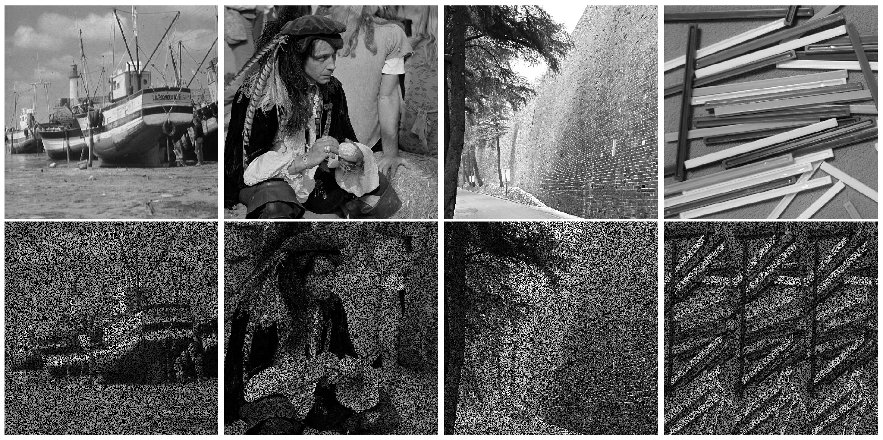
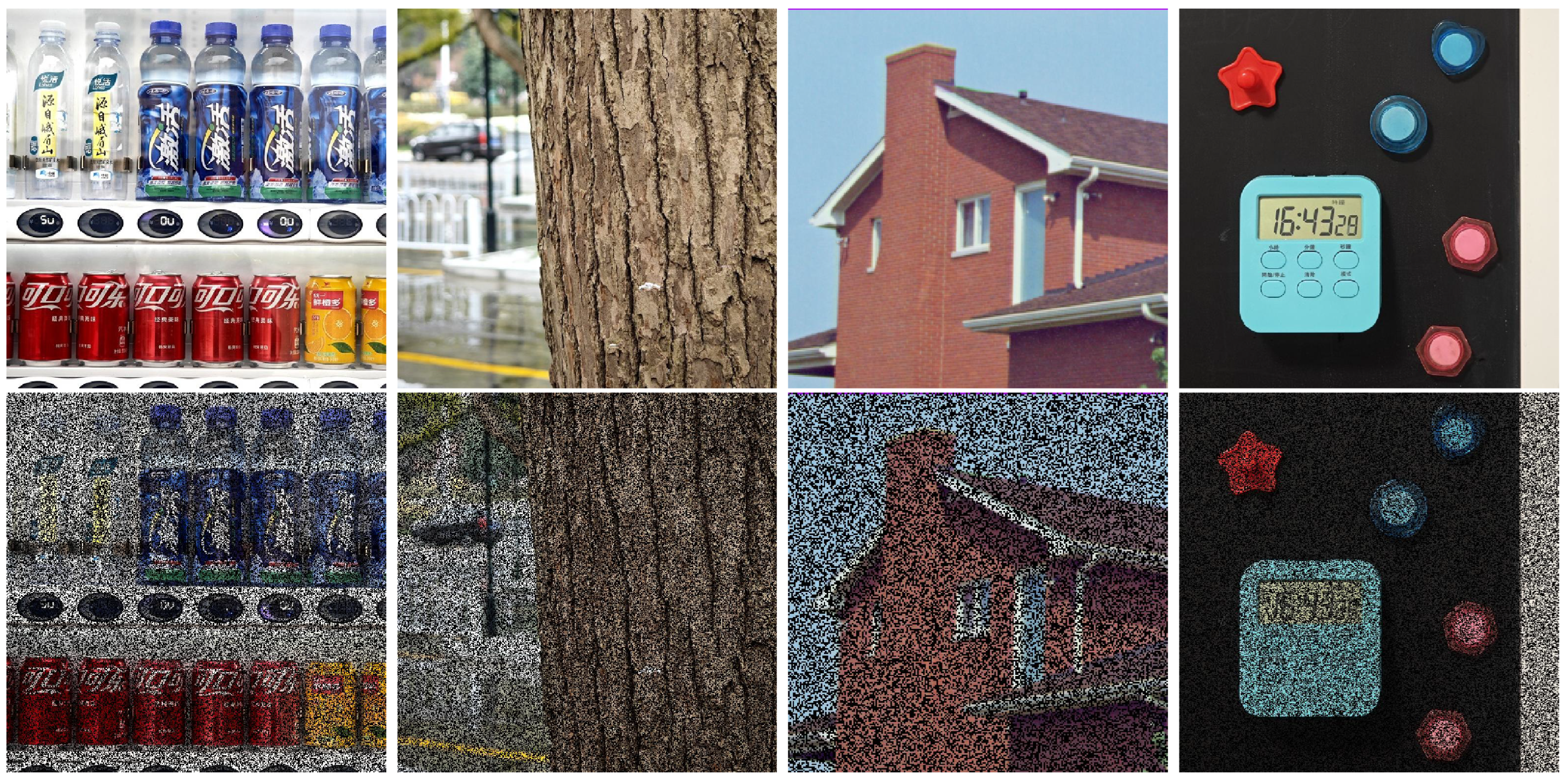
To more comprehensively demonstrate algorithmic efficacy, we constructed four 2D images, “Boat ( 512 × 512 )”, “Man ( 1024 × 1024 )”, “City Wall ( 512 × 512 )” and “Spillikins ( 512 × 512 )”, alongside four 3D counterparts, “Bottles ( 512 × 512 )”, “Texture ( 512 × 512 )”, “House ( 256 × 256 )”, “Clock ( 512 × 512 )”, visualized in Figure 2 and Figure 3. It is universally acknowledged that although not all authentic images possess low-rank characteristics, the essential information is primarily determined by the higher singular values. Consequently, it is feasible to recover corrupted images through low-rank approximation. For 3D imagery containing three separate channels, matrix completion executes independently per channel. The approach for selecting parameters remains identical to that employed in the artificial example, and the termination criterion is P Ω ( X ) Y 10 3 .
Due to space constraints, we concentrate upon the ETP penalty function to demonstrate recovery efficacy. The algorithm’s recovery capability quantifies via Signal-to-Noise Ratio (SNR), defined as
SNR ( u , u ¯ ) = 10 log 10 u u ¯ 2 u u 2 ,
where u and u ¯ signify the original image and mean of the original image, and u the reconstructed image.
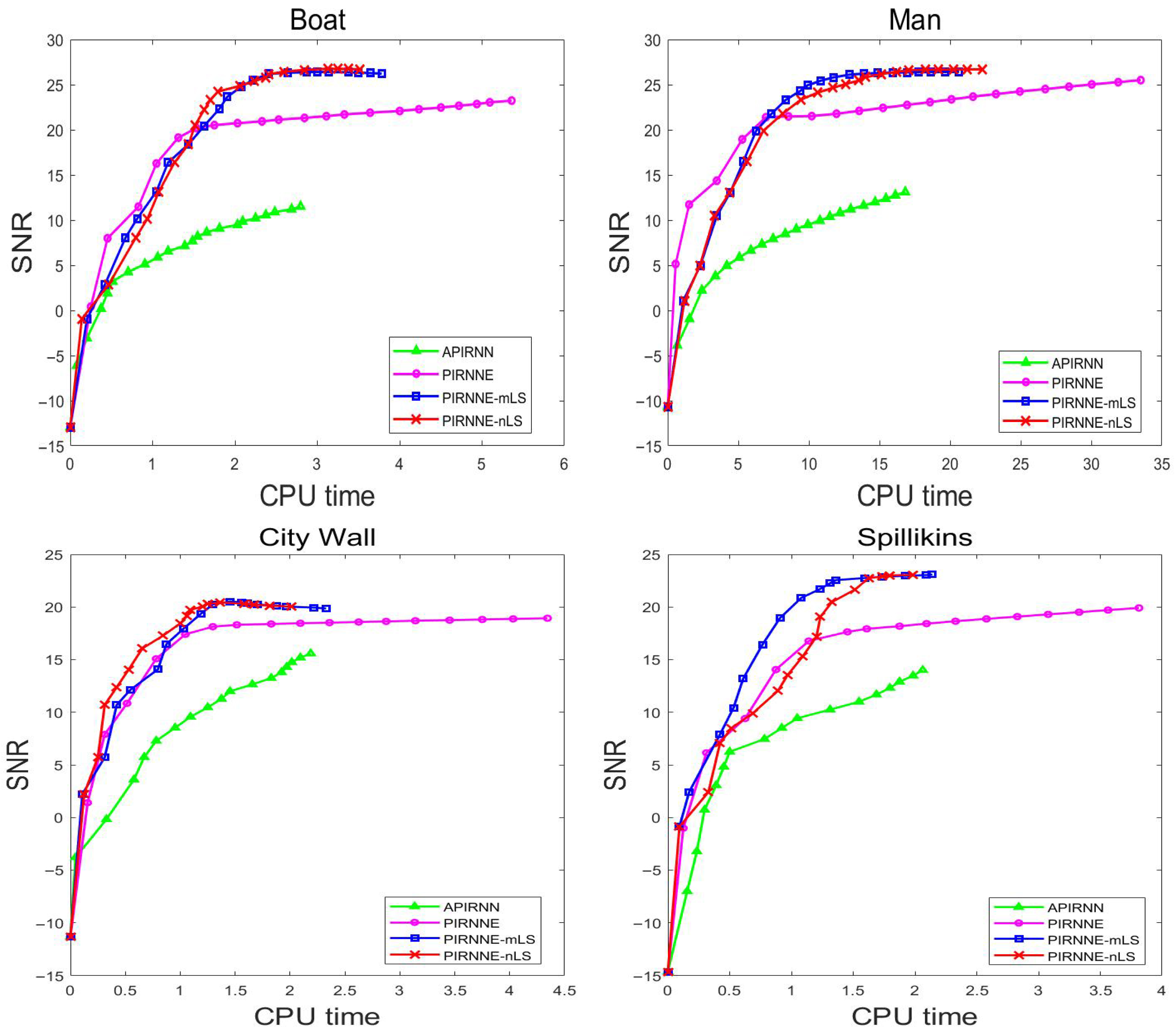
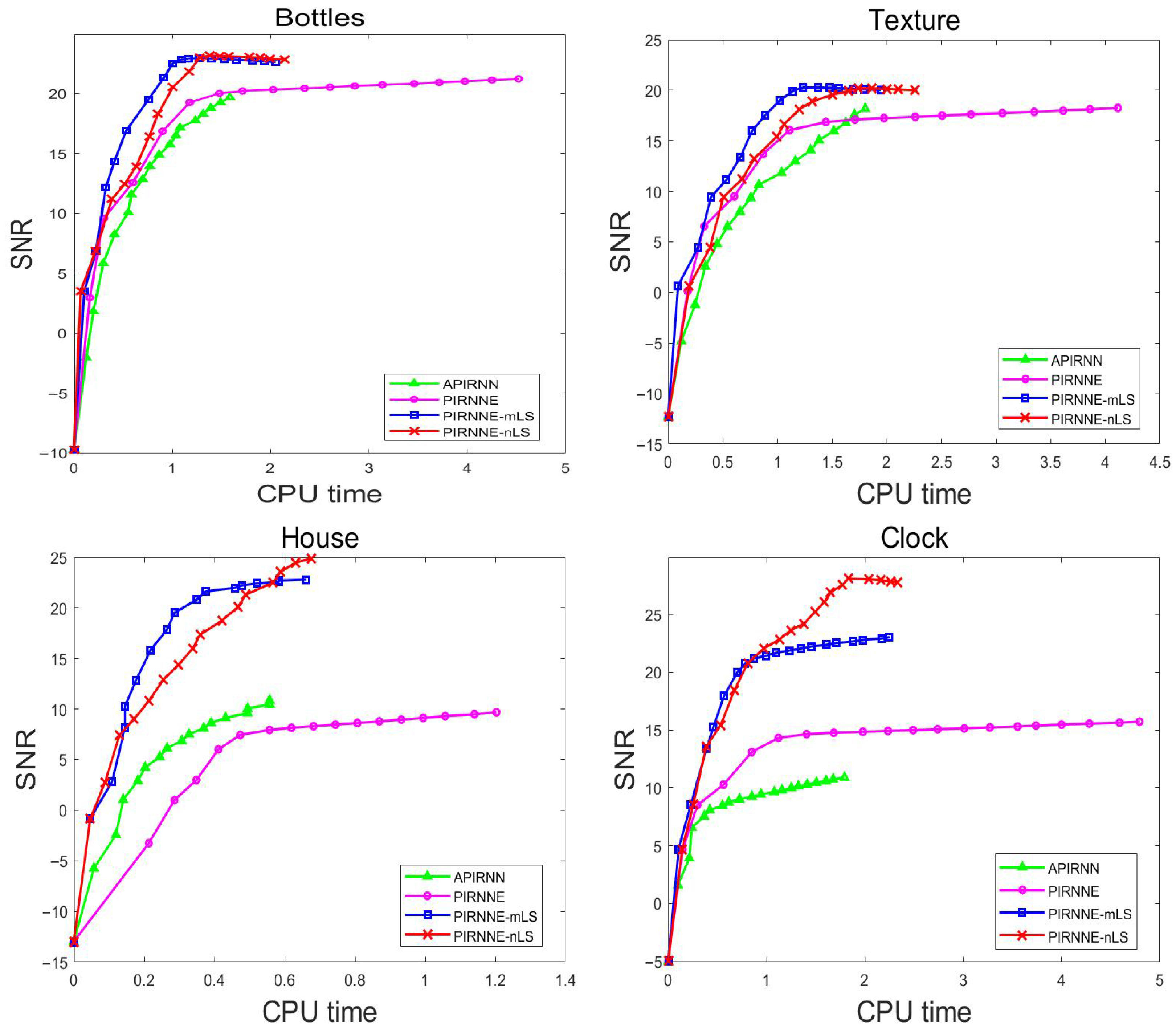
For this evaluation, random values perturb 50 % of image elements, with Ω denoting a set of random values. These corrupted images appear in Figure 2 and Figure 3’s second row. SNR values relative to CPU duration—required by four methods to attain minimal processing time—are plotted across Figure 4 and Figure 5. The results in Figure 4 and Figure 5 show that PIRNNE-LS (including PIRNNE-mLS and PIRNNE-nLS) outperforms traditional APIRNN and PIRNNE.
Furthermore, we report the number of iterations and CPU time in seconds and SNR values in Table 1. In the presented results, we use “Iter.”, “Time” and “SNR” to denote the number of iterations, CPU time in seconds and SNR value, respectively. In color images, Iter., Time and SNR represent the mean values of the three channels. From Table 1, we observe that our proposed PIRNNE-mLS and PIRNNE-nLS have better recovery performance.

5.3. Movie Recommendation System

In order to further evaluate the performance of the proposed algorithm, we test our algorithm on the MovieLens dataset [41]. MovieLens dataset contains anonymous ratings of movies by users. Three subsets of the dataset are employed: 100 K, 1 M and 10 M, with varying numbers of users, movies and ratings as described in Table 2.
The experiments were conducted on a workstation equipped with an Intel Xeon Gold 5218R processor (20 cores/40 threads), 64 GB of RAM and dual NVIDIA GeForce RTX 4090 GPU. The software environment is Ubuntu 22.04.4 LTS and MATLAB R2020a. The key measuring metrics are computational efficiency via GPU seconds (Time), recovery accuracy via RMSE and the objective value, which are adopted to determine the algorithm’s superiority. The comparative results of different algorithms on the MovieLens dataset subsets are presented in Table 3. It should be emphasized that our advantages are not apparent with small data. However, our algorithms have a marked advantage with big data.

6. Conclusions

This paper addresses a class of nonconvex and nonsmooth optimization problems that are commonly encountered in various applications. Based on existing dimension reduction and extrapolation techniques, we propose a more generalized proximal iterative reweighted nuclear norm method. This method utilizes a line search mechanism to avoid parameter constraints, thereby providing greater flexibility in parameter selection. As a result, it is feasible to expand the application of this method in the future. In theory, we prove the subsequential convergence. Furthermore, for the case of monotone line search, we prove the global convergence and linear convergence rate of the algorithm under the KL framework. Finally, we validate the effectiveness of the algorithm through numerical results on synthetic and real data. We will construct a new nonconvex optimization model with distributed characteristics and design corresponding algorithms [42,43] based on the low rank of matrix. This will be our future research work.

Author Contributions

Conceptualization, Z.G.; methodology, Z.G.; formal analysis, Z.G.; writing—original draft preparation, Z.G.; software, X.Z.; validation, X.Z. and S.Z.; writing—review and editing, Z.G., S.Z., X.Z. and Y.C.; visualization, X.Z. and S.Z. All authors have read and agreed to the published version of the manuscript.

Funding

This research was funded by the National Natural Science Foundation of China (12471290), Natural Science Research of the Jiangsu Higher Education Institutions of China (20KJA520003), Six Talent Peaks Project of Jiangsu Province (JY-051), Open Fund of the Key Laboratory of NSLSCS, Ministry of Education, Suqian Sci&Tech Program (M202206) and Qing Lan Project.

Data Availability Statement

The original contributions presented in this study are included in the article. Further inquiries can be directed to the corresponding author.

Conflicts of Interest

The authors declare no conflicts of interest.

References

  1. Ge, Z.L.; Zhang, X.; Wu, Z.M. A fast proximal iteratively reweighted nuclear norm algorithm for nonconvex low-rank matrix minimization problems. Appl. Numer. Math. 2022, 179, 66–86. [Google Scholar] [CrossRef]
  2. Argyriou, A.; Evgeniou, T.; Pontil, M. Convex multi-task feature learning. Mach. Learn. 2008, 73, 243–272. [Google Scholar] [CrossRef]
  3. Amit, Y.; Fink, M.; Srebro, N.; Ullman, S. Uncovering shared structures in multiclass classification. In Proceedings of the the 24th International Conference on Machine Learning, Corvallis, OR, USA, 20–24 June 2007. [Google Scholar] [CrossRef]
  4. Lu, C.Y.; Tang, J.H.; Yan, S.C.; Lin, Z.C. Generalized nonconvex nonsmooth low-rank minimization. In Proceedings of the 2014 IEEE Conference on Computer Vision and Pattern Recognition, Columbus, OH, USA, 23–28 June 2014; IEEE Computer Society: Washington, DC, USA, 2014; pp. 4130–4137. [Google Scholar]
  5. Dong, W.S.; Shi, G.M.; Li, X.; Ma, Y.; Huang, F. Compressive sensing via nonlocal low-rank regularization. IEEE Trans. Image Process. 2014, 23, 3618–3632. [Google Scholar] [CrossRef]
  6. Fazel, M.; Hindi, H.; Boyd, S.P. Log-det heuristic for matrix rank minimization with applications to Hankel and Euclidean distance matrices. In Proceedings of the 2003 American Control Conference, Denver, CO, USA, 4–6 June 2003; IEEE: New York, NY, USA, 2003; pp. 2156–2162. [Google Scholar]
  7. Hu, Y.; Zhang, D.B.; Ye, J.P.; Li, X.L.; He, X.F. Fast and accurate matrix completion via truncated nuclear norm regularization. IEEE Trans. Pattern Anal. 2013, 35, 2117–2130. [Google Scholar] [CrossRef]
  8. Lu, C.Y.; Zhu, C.B.; Xu, C.Y.; Yan, S.C.; Lin, Z.C. Generalized singular value thresholding. In Proceedings of the 29th AAAI Conference on Artificial Intelligence, Austin, TX, USA, 25–30 January 2015; pp. 1215–1221. [Google Scholar] [CrossRef]
  9. Todeschini, A.; Caron, F.; Chavent, M. Probabilistic low-rank matrix completion with adaptive spectral regularization algorithms. Adv. Neural Inf. Process. Syst. 2013, 26, 845–853. [Google Scholar]
  10. Toh, K.C.; Yun, S.W. An accelerated proximal gradient algorithm for nuclear norm regularized linear least squares problems. Pac. J. Optim. 2010, 6, 615–640. [Google Scholar]
  11. Zhang, X.; Peng, D.T.; Su, Y.Y. A singular value shrinkage thresholding algorithm for folded concave penalized low-rank matrix optimization problems. J. Glob. Optim. 2024, 88, 485–508. [Google Scholar] [CrossRef]
  12. Tao, T.; Xiao, L.H.; Zhong, J.Y. A Fast Proximal Alternating Method for Robust Matrix Factorization of Matrix Recovery with Outliers. Mathematics 2025, 13, 1466. [Google Scholar] [CrossRef]
  13. Cui, A.G.; He, H.Z.; Yuan, H. A Designed Thresholding Operator for Low-Rank Matrix Completion. Mathematics 2024, 12, 1065. [Google Scholar] [CrossRef]
  14. Gong, P.H.; Zhang, C.S.; Lu, Z.S.; Huang, J.H.Z.; Ye, J.P. A general iterative shrinkage and thresholding algorithm for non-convex regularized optimization problems. In Proceedings of the 30th International Conference on Machine Learning, Atlanta, GA, USA, 16–21 June 2013; pp. 37–45. [Google Scholar]
  15. Nakayama, S.; Narushima, Y.; Yabe, H. Inexact proximal DC Newton-type method for nonconvex composite functions. Comput. Optim. Appl. 2024, 87, 611–640. [Google Scholar] [CrossRef]
  16. Sun, T.; Jiang, H.; Cheng, L.Z. Convergence of proximal iteratively reweighted nuclear norm algorithm for image processing. IEEE Trans. Image Process. 2017, 26, 5632–5644. [Google Scholar] [CrossRef]
  17. Phan, D.N.; Nguyen, T.N. An accelerated IRNN-Iteratively Reweighted Nuclear Norm algorithm for nonconvex nonsmooth low-rank minimization problems. J. Comput. Appl. Math. 2021, 396, 113602. [Google Scholar] [CrossRef]
  18. Xu, Z.Q.; Zhang, Y.L.; Ma, C.; Yan, Y.C.; Peng, Z.L.; Xie, S.L.; Wu, S.Q.; Yang, X.K. LERE: Learning-Based Low-Rank Matrix Recovery with Rank Estimation. In Proceedings of the 38th AAAI Conference on Artificial Intelligence, Vancouver, BC, Canada, 20–27 February 2024; pp. 16228–16236. [Google Scholar] [CrossRef]
  19. Wen, Y.W.; Li, K.X.; Chen, H.F. Accelerated matrix completion algorithm using continuation strategy and randomized SVD. J. Comput. Appl. Math. 2023, 429, 115215. [Google Scholar] [CrossRef]
  20. Zhang, H.M.; Qian, F.; Shi, P.; Du, W.L.; Tang, Y.; Qian, J.J.; Gong, C.; Yang, J. Generalized Nonconvex Nonsmooth Low-Rank Matrix Recovery Framework With Feasible Algorithm Designs and Convergence Analysis. IEEE Trans. Neur. Net. Lear. 2023, 34, 5342–5353. [Google Scholar] [CrossRef] [PubMed]
  21. Li, B.J.; Pan, S.H.; Qian, Y.T. Factorization model with total variation regularizer for image reconstruction and subgradient algorithm. Pattern Recogn. 2026, 170, 112038. [Google Scholar] [CrossRef]
  22. Guo, H.Y.; Huang, Z.H.; Zhang, X.Z. Low rank matrix recovery with impulsive noise. Appl. Math. Lett. 2022, 134, 108364. [Google Scholar] [CrossRef]
  23. Wang, H.; Wang, Y.; Yang, X.Y. Efficient Active Manifold Identification via Accelerated Iteratively Reweighted Nuclear Norm Minimization. J. Mach. Learn. Res. 2024, 25, 1–44. [Google Scholar]
  24. Beck, A.; Teboulle, M. A fast iterative shrinkage-thresholding algorithm for linear inverse problems. SIAM J. Imaging Sci. 2009, 2, 183–202. [Google Scholar] [CrossRef]
  25. Li, H.; Lin, Z.C. Accelerated proximal gradient methods for nonconvex programming. Adv. Neural Inf. Process. Syst. 2015, 28, 377–387. [Google Scholar]
  26. Grippo, L.; Lampariello, F.; Lucidi, S. A nonmonotone line search technique for Newton’s method. SIAM J. Numer. Anal. 1986, 23, 707–716. [Google Scholar] [CrossRef]
  27. Wright, S.J.; Nowak, R.; Figueiredo, M.A.T. Sparse reconstruction by separable approximation. IEEE Trans. Signal Process. 2008, 57, 2479–2493. [Google Scholar] [CrossRef]
  28. Wu, Z.M.; Li, C.S.; Li, M.; Andrew, L. Inertial proximal gradient methods with Bregman regularization for a class of nonconvex optimization problems. J. Glob. Optim. 2021, 79, 617–644. [Google Scholar] [CrossRef]
  29. Liu, J.Y.; Cui, Y.; Pang, J.S.; Sen, S. Two-stage stochastic programming with linearly bi-parameterized quadratic recourse. SIAM J. Optimiz. 2020, 30, 2530–2558. [Google Scholar] [CrossRef]
  30. Wang, J.Y.; Petra, C.G. A sequential quadratic programming algorithm for nonsmooth problems with upper-C2 Objective. SIAM J. Optimiz. 2023, 33, 2379–2405. [Google Scholar] [CrossRef]
  31. Yang, L. Proximal gradient method with extrapolation and line search for a class of nonconvex and nonsmooth problems. J. Optimiz. Theory App. 2024, 200, 68–103. [Google Scholar] [CrossRef]
  32. Attouch, H.; Bolte, J.; Svaiter, B.F. Convergence of descent methods for semi-algebraic and tame problems: Proximal algorithms, forward-backward splitting, and regularized Gauss-Seidel methods. Math. Program. 2013, 137, 91–129. [Google Scholar] [CrossRef]
  33. Bolte, J.; Sabach, S.; Teboulle, M. Proximal alternating linearized minimization for nonconvex and nonsmooth problems. Math. Program. 2014, 146, 459–494. [Google Scholar] [CrossRef]
  34. Kurdyka, K. On gradients of functions definable in o-minimal structures. Ann. I. Fourier 1998, 48, 769–783. [Google Scholar] [CrossRef]
  35. Attouch, H.; Bolte, J.; Redont, P.; Soubeyran, A. Proximal alternating minimization and projection methods for nonconvex problems: An approach based on the Kurdyka-Lojasiewicz inequality. Math. Oper. Res. 2010, 35, 438–457. [Google Scholar] [CrossRef]
  36. Ge, Z.L.; Wu, Z.M.; Zhang, X. An extrapolated proximal iteratively reweighted method for nonconvex composite optimization problems. J. Glob. Optim. 2023, 86, 821–844. [Google Scholar] [CrossRef]
  37. Guo, K.; Han, D.R. A note on the Douglas-Rachford splitting method for optimization problems involving hypoconvex functions. J. Glob. Optim. 2018, 72, 431–441. [Google Scholar] [CrossRef]
  38. Wen, B.; Chen, X.J.; Pong, T.K. Linear convergence of proximal gradient algorithm with extrapolation for a class of nonconvex nonsmooth minimization problems. SIAM J. Optimiz. 2017, 27, 124–145. [Google Scholar] [CrossRef]
  39. Wu, Z.M.; Li, M. General inertial proximal gradient method for a class of nonconvex nonsmooth optimization problems. Comput. Optim. Appl. 2019, 73, 129–158. [Google Scholar] [CrossRef]
  40. Nesterov, Y. Introductory Lectures on Convex Optimization: A Basic Course; Springer: New York, NY, USA, 2013. [Google Scholar] [CrossRef]
  41. Harper, F.M.; Konstan, J.A. The MovieLens Datasets: History and Context. ACM TiiS 2015, 5, 1–19. [Google Scholar] [CrossRef]
  42. Li, S.; Li, Q.W.; Zhu, Z.H.; Tang, G.G.; Wakin, M.B. The global geometry of centralized and distributed low-rank matrix recovery without regularization. IEEE Signal Proc. Let. 2020, 27, 1400–1404. [Google Scholar] [CrossRef]
  43. Doostmohammadian, M.; Gabidullina, Z.R.; Rabiee, H.R. Nonlinear perturbation-based non-convex optimization over time-varying networks. IEEE Trans. Netw. Sci. Eng. 2024, 11, 6461–6469. [Google Scholar] [CrossRef]
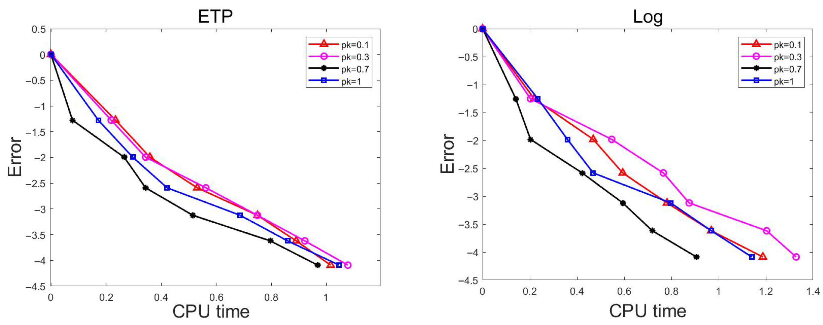
Figure 1. Evolution of the error value with respect to the CPU time.
Mathematics 13 02630 g001
Figure 2. The list of pictures in order: Boat, Man, City Wall and Spillikins. First row: original images, second row: noisy images.
Mathematics 13 02630 g002
Figure 3. The list of pictures in order: Bottles, Texture, House and Clock. First row: original images, second row: noisy images.
Mathematics 13 02630 g003
Figure 4. Evolution of SNR values of Boat, Man, City Wall and Spillikins with respect to the CPU time.
Mathematics 13 02630 g004
Figure 5. Evolution of SNR values of Bottles, Texture, House and Clock with respect to the CPU time.
Mathematics 13 02630 g005
Table 1. Numerical results of tested algorithms with Boat, Man, City Wall, Spillikins, Bottles, Texture, House and Clock.
APIRNNPIRNNEPIRNNE-mLSPIRNNE-nLS
Iter.TimeSNRIter.TimeSNRIter.TimeSNRIter.TimeSNR
Boat1213.9419.49512.8723.96431.9026.23431.9026.69
Man11730.0223.295623.9026.644515.6126.354415.4126.79
City Wall561.4317.88401.6119.08381.0519.74350.9620.05
Spillikins681.5720.05591.9622.39341.0323.08331.0123.09
Bottles664.7621.92566.3422.26463.1022.50382.9822.74
Texture574.7219.81526.0919.55423.1320.94352.8021.95
House1091.1721.961142.7421.37390.5823.94380.5524.76
Clock22912.1020.4315517.3624.92555.0124.28473.3027.99
Table 2. Dataset descriptions. The number of users, items and ratings used in each dataset.
Dataset UsersMoviesRatings
MovieLens100 K9431682100,000
1 M60403449999,714
10 M69,87810,67710,000,054
Table 3. Comparative results of tested algorithms on the MovieLens dataset subsets.
Dataset MethodTimeRMSEObjective Value
MovieLens100 KAPIRNN2.061.0410 6.4081 × 10 2
PIRNNE1.111.0216 7.8860 × 10 2
PIRNNE-mLS2.001.0468 5.9634 × 10 2
PIRNNE-nLS1.981.0450 6.1770 × 10 2
1 MAPIRNN6.240.8855 1.1575 × 10 5
PIRNNE7.881.0343 1.2641 × 10 5
PIRNNE-mLS5.230.8844 1.0311 × 10 5
PIRNNE-nLS5.220.8844 1.0311 × 10 5
10 MAPIRNN28.230.9483 1.9444 × 10 6
PIRNNE238.861.0063 2.1513 × 10 6
PIRNNE-mLS14.490.9483 1.9435 × 10 6
PIRNNE-nLS13.780.9483 1.9435 × 10 6
Disclaimer/Publisher’s Note: The statements, opinions and data contained in all publications are solely those of the individual author(s) and contributor(s) and not of MDPI and/or the editor(s). MDPI and/or the editor(s) disclaim responsibility for any injury to people or property resulting from any ideas, methods, instructions or products referred to in the content.