Model Reduction in Parallelization Based on Equivalent Transformation of Block Bi-Diagonal Toeplitz Matrices for Two-Dimensional Discrete-Time Systems

Abstract

This study proposes a parallel model reduction method for two-dimensional discrete-time systems, utilizing Krawtchouk moments and equivalent transformation. This work makes two significant contributions. First, we introduce a projection subspace that is independent of the input as well as of the Krawtchouk parameters, thus ensuring robustness. Second, we propose an efficient parallel algorithm for computing the basis of the projection subspace. With the difference relation of Krawtchouk polynomials and the analytic identity theorem, we obtain the explicit formula for the Krawtchouk moments of the state, which is input-dependent and Krawtchouk-parameter-dependent. We derive a projection subspace that is independent of both input and Krawtchouk parameter, such that it is equivalent to the subspace spanned by the Krawtchouk moments. Further, we propose a parallel strategy based on the equivalent transformation of the block bi-diagonal Toeplitz matrices with bi-diagonal blocks to compute the basis of the projection subspace, facilitating acceleration of the model reduction process on high-performance computers. Moreover, we analyze the Krawtchouk moment invariants of the proposed parallel method. Finally, the effectiveness of the proposed method is illustrated by two numerical examples.

1. Introduction

In virtually all scientific and engineering disciplines, mathematical modelling of physical systems often leads to complex high-order systems, described by large-scale differential or difference equations [1,2,3,4]. Direct simulation of these complex high-order systems is generally not recommended due to the excessive computational burden. Consequently, in practical applications, it is desirable to design a lower-order system to replace the high-order system according to certain given criteria. Model reduction is a powerful tool for generating a lower-order model that accurately approximates the responses of the original system while preserving important dynamical properties [5,6,7,8,9]. Such a reduced system serves as an efficient alternative for analysis, control, and synthesis. Over the past few decades, extensive research has been conducted on model reduction for one-dimensional systems, encompassing a variety of efficient techniques, such as the balanced truncation methods [10,11,12,13,14], the moment matching methods [15], the orthogonal polynomial methods [16,17], the optimal model reduction methods [18,19,20,21,22] and so on.

Multi-dimensional systems, governed by differential equations or difference equations, arise naturally in various engineering applications, including control theory and signal processing [23,24]. As a special case, the analysis and synthesis of two-dimensional systems have received much attention and have been extensively studied. This kind of system represents the propagation in two independent directions, which occur in various engineering fields [25,26]. To represent a two-dimensional system in the state-space form, several generalized descriptions are presented in literature, where the well known ones are the Roesser model [25] and the Fornasini-Machesini local state-space (FMLSS) model [26]. The analysis, simulation, and design of two-dimensional systems are challenging due to their two-dimensional variables, which introduce significant difficulty and complexity.

However, many established results for one-dimensional systems are not directly applicable to two-dimensional systems. Numerous researchers are dedicated to investigating model reduction for two-dimensional systems and have proposed various effective methods. For two-dimensional filters, the concepts of local reachability and observability are initially defined, and the reachable and observable realizations are subsequently discussed [27]. In addition, the generalizations of reachability and observability Gramians to two-dimensional discrete-time systems are explored in [28]. Based on the two-dimensional Gramians, the balanced realization of two-dimensional discrete-time systems is proposed and the frequency error bounds for reduced systems are given [29]. For two-dimensional discrete-time systems with separable denominators, balanced truncation methods based on frequency-domain interval Gramians are proposed [30,31]. In addition, ${\mathcal{H}}_{\infty }$ model reduction techniques are proposed for handling two-dimensional discrete-time systems. For two-dimensional discrete-time systems described by the Roesser model, the literature [32] solves the ${\mathcal{H}}_{\infty }$ model reduction problem by using the linear matrix inequality (LMI) technique, and the solvability conditions for the two-dimensional reduced systems are derived. Besides, the ${\mathcal{H}}_{\infty }$ model reduction problem for two-dimensional discrete-time systems with parameter uncertainty is discussed in [33]. To enhance the approximation performance over a specific frequency interval, the authors in [34] explore the generalized ${\mathcal{H}}_{\infty }$ model reduction for stable two-dimensional discrete-time systems, where the resulting reduced models are stable and have a prescribed generalized ${\mathcal{H}}_{\infty }$ performance index.

Orthogonal polynomial-based methods have been studied for different kinds of dynamical systems, such as bilinear systems [35], time-delay systems [17,36,37], and parametric system [38,39,40]. These literatures have demonstrated the effectiveness and practicability of orthogonal polynomial methods. The inherent orthogonality and compact representation of polynomial moments make them particularly suitable for devoloping the model reduction methods for discrete-time systems. Specifically, the model reduction methods based on the polynomial moment derived from bivariate discrete orthogonal polynomials are proposed for two-dimensional discrete-time systems [41]. However, the current orthogonal polynomial-based methods typically construct projection subspaces by solving large-scale linear systems for the expansion coefficients, which leads to significant computational burden. Moreover, the resulting reduced systems may exhibit sensitivity to variations in inputs and polynomial parameters, potentially compromising their robustness. This implies that the selection of inputs and polynomial parameters can affect the result of the reduced systems, which may introduce ambiguity regarding the optimal choices for inputs and polynomial parameters.

Motivated by this, we propose a parallel model reduction method based on the Krawtchouk moments and the equivalent transformation of block bi-diagonal Toeplitz matrix for two-dimensional discrete-time systems. The present work comprises two primary contributions: the construction of an input-independent and Krawtchouk-parameter-independent projection subspace, and the development of a parallel strategy to compute the basis of the projection subspace. Utilizing the difference relation of Krawtchouk polynomials, the forward terms in the two-dimensional discrete-time system are approximated in the subspace spanned by bivariate discrete-time polynomials with the product of Krawtchouk polynomials. By applying the analytic identity theorem, we obtain the explicit formula related to the Krawtchouk moments of the state, which is input-dependent and Krawtchouk-parameter-dependent. By analyzing the subspace spanned by the Krawtchouk moments, we prove that this subspace is equivalent to the subspace spanned by a sequence of input-independent and Krawtchouk-parameter-independent vectors. By iteratively computing these vectors, the projection matrix is obtained to reduce the original system. However, with the increase of the scale of the original system, this process will cause the huge computational burden. For this, we further investigate the parallel strategy for computing the bases of the projection subspace. By defining two scaling matrices and using the block diagonalization technique, a parallel strategy is proposed to equivalently solve the linear equations and compute the basis of the projection subspace. The parallel strategy enables the transformation of the block bi-diagonal Toeplitz matrices into a block-diagonal form, facilitating the decoupling of computations of the basis of the projection subspace. This structural transformation allows for independent and concurrent processing of each block, significantly enhancing the method’s parallelizability and computational efficiency. This also enables acceleration of the model reduction process using high performance computers. Theoretical analysis shows that the resulting reduced system can preserve the first several Krawtchouk moments of the original system. Finally, the numerical experiment is given to demonstrate the efficiency of the proposed method.

The structure of this paper is as follows. In Section 2, we review essential definitions and properties of Krawtchouk polynomials and Krawtchouk moments, and formally formulate the model reduction problem addressed in this study. In Section 3, we present a parallel model reduction method for two-dimensional discrete-time systems that is independent of both the inputs and the Krawtchouk parameters. And we also analyze the properties of the proposed method in this section. Numerical experiments are presented to illustrate the effectiveness of the proposed methods in Section 4. We end the paper with a short conclusion and discussion in Section 5.

Notations: Throughout the paper, we adopt the notational conventions commonly used in matrix computation literature. Specifically, $I_k$ denotes the $k\times k$ identity matrix, $A^T$ denotes the transpose of the matrix A. We use $\left({\displaystyle \genfrac{}{}{0pt}{}{i}{j}}\right)$ to denote binomial coefficients and use ${\left(i\right)}_j$ to denote Pochhammer’s symbol, which is defined by ${\left(i\right)}_j=(i+j-1)(i+j-2)\cdots (i+1)i$ for $j\ge 1$ and ${\left(i\right)}_j=1$ for $j=0$. We use $\mathrm{span}\{a_0,a_1,\cdots ,a_{r-1}\}$ to denote the space spanned by the vectors $a_i$ with $i=0,1,\cdots ,r-1$, and apply $\mathrm{colspan}\left\{V\right\}$ to denote the space spanned by the columns of V. For the constants i and $j<i$, we denote the matrix $H_{i,j}=\left[\begin{array}{cc}0& 0\\ I_{i-j}& 0\end{array}\right]\in {\mathbb{R}}^{i\times i}$.

2. Preliminaries

This section commences with a presentation of the fundamental definitions and mathematical properties underlying Krawtchouk polynomials. Subsequently, the notion of Krawtchouk moments is defined through orthogonal projection operations in the subspace spanned by bivariate discrete-time polynomials. After that, we formulate the model reduction problem for two-dimensional discrete-time systems.

2.1. Krawtchouk Polynomials and Krawtchouk Moments

In this section, we present an overview of the essential concepts and expressions associated with Krawtchouk polynomials and revisit the definition of Krawtchouk moments. For further details on Krawtchouk polynomials, one can refer to [39,42,43]. The k-th order Krawtchouk polynomial is defined as follows

$${\mathcal{K}}_k(i;p_K,N_K)={(-p_K)}^k\left({\displaystyle \genfrac{}{}{0pt}{}{N_K}{k}}\right){}_{2}F_1\left(-k,-i,-N_K;{\displaystyle \frac{1}{p_K}}\right)$$

where $i,k=0,1,\cdots ,N_K$, $N_K>0$, and $p_K\in (0,1)$ is the Krawtchouk parameter. Here, ${}_{2}F_1$ is the hypergeometric function and defined as

$${}_{2}F_1\left(a,b,c;z\right)=\sum _{k=0}^{+\infty }{\displaystyle \frac{{\left(a\right)}_k{\left(b\right)}_k}{{\left(c\right)}_k}}{\displaystyle \frac{z^k}{k!}}.$$

The set of $(N_K+1)$ Krawtchouk polynomials forms a complete set of discrete basis functions with weight function

$$\omega (i;p_K,q_K,N_K)=\left({\displaystyle \genfrac{}{}{0pt}{}{N_K}{i}}\right)p_K^i{q}_K^{N_K-i},$$

where $q_K=1-p_K$. These polynomials satisfy the orthogonality relation

$$\sum _{i=0}^{N_K}\omega (i;p_K,q_K,N_K){\mathcal{K}}_k(i;p_K,N_K){\mathcal{K}}_l(i;p_K,N_K)=\rho (k,p_K,q_K,N_K){\delta }_{kl},$$

for all $k,l=0,1,\cdots ,N_K$, where ${\delta }_{kl}$ is the Kronecker delta function, and

$$\rho (k,p_K,q_K,N_K)=\left({\displaystyle \genfrac{}{}{0pt}{}{N_K}{k}}\right)p_K^k{q}_K^k.$$

From [43], the difference relation for the Krawtchouk polynomials is represented by the forward difference operator, denoted as ${\Delta }_{+}$, and is expressed as:

$${\Delta }_{+}{\mathcal{K}}_k(i;p_K,N_K)={\mathcal{K}}_{k-1}(i;p_K,N_K-1),$$

(1)

where ${\Delta }_{+}{\mathcal{K}}_k(i;p_K,N_K)={\mathcal{K}}_k(i+1;p_K,N_K)-{\mathcal{K}}_k(i;p_K,N_K)$. This relation reveals a recursive structure inherent to the Krawtchouk polynomials. However, the difference relation of Krawtchouk polynomials contains ${\mathcal{K}}_{k-1}(i;p_K,N_K-1)$ about $N_K-1$, which poses a challenge when attempting to directly obtain the expansion coefficients required for model reduction processes. To address this, the explicit difference relation is derived in [38], i.e.,

$${\Delta }_{+}{\mathcal{K}}_k(i;p_K,N_K)=\sum _{s=0}^{k-1}{p}_K^s{\mathcal{K}}_{k-s-1}(i;p_K,N_K).$$

(2)

Krawtchouk moments have extensive applications in the field of image processing. For the functions with two-dimensional variables, we present a brief introduction about the extended definition of Krawtchouk moments. For simplicity, we denote the bivariate discrete-time polynomials with the product of Krawtchouk polynomials ${\mathcal{K}}_k(i;p_K,N_K){\mathcal{K}}_l(j;p_K,N_K)$ as ${\mathcal{K}}_{k,l}^{i,j}$, where $k,l=0,1,\dots ,N_K$. For the function $f(i,j)$ with the discrete-time variables $i,j$, it can be expanded in the subspace spanned by bivariate discrete-time polynomials with the product of Krawtchouk polynomials, i.e.,

$$f(i,j)=\sum _{k=0}^{N_K}\sum _{l=0}^{N_K}{f}_{k,l}{\mathcal{K}}_{k,l}^{i,j},$$

where $f_{k,l}$ is defined as the Krawtchouk moments of the function $f(i,j)$ and computed by

$$f_{k,l}=\sum _{i=0}^{N_K}\sum _{j=0}^{N_K}{\displaystyle \frac{\omega (i;p_K,q_K,N_K)\omega (j;p_K,q_K,N_K)}{\rho (k,p_K,q_K,N_K)\rho (l,p_K,q_K,N_K)}}{\mathcal{K}}_{k,l}^{i,j}f(i,j).$$

This expansion allows for the efficient representation of the function $f(i,j)$ in terms of its Krawtchouk moments, which can be used for model reduction of two-dimensional systems.

2.2. Model Reduction Problem of Two-Dimensional Discrete-Time Systems

Consider the two-dimensional discrete-time system described by FMLSS model in the states of the form

$$\left\{\begin{array}{cc}\hfill x(i+1,j+1)& =A_{1}x(i,j+1)+A_{2}x(i+1,j)+B_{1}u(i,j+1)+B_{2}u(i+1,j),\hfill \\ \hfill y(i,j)& =Cx(i,j)+Du(i,j),\hfill \end{array}\right.$$

(3)

where $A_1,A_2\in {\mathbb{R}}^{n\times n}$, $B_1,B_2\in {\mathbb{R}}^{n\times p}$, $C\in {\mathbb{R}}^{q\times n}$, and $D\in {\mathbb{R}}^{q\times p}$. The variable $x(i,j)\in {\mathbb{R}}^n$ is the state, $u(i,j)\in {\mathbb{R}}^p$ is the input which belongs to $l_2\{[0,+\infty ),[0,+\infty )\}$, and $y(i,j)\in {\mathbb{R}}^q$ is the output.

In this paper, we aim to explore the time-domain model reduction method based on the Galerkin projection. Concretely, we first construct a projection subspace defined by the projection matrix $V\in {\mathbb{R}}^{n\times r}$ with $V^{T}V=I_r$. Then, the solution $x(i,j)$ is approximated in the subspace spanned by the columns of V, i.e., $x(i,j)\approx V\widehat{x}(i,j)$. Consequently, we obtain

$$\left\{\begin{array}{cc}\hfill \widehat{x}(i+1,j+1)& ={\widehat{A}}_1\widehat{x}(i,j+1)+{\widehat{A}}_2\widehat{x}(i+1,j)+{\widehat{B}}_{1}u(i,j+1)+{\widehat{B}}_{2}u(i+1,j),\hfill \\ \hfill \widehat{y}(i,j)& =\widehat{C}\widehat{x}(i,j)+\widehat{D}u(i,j),\hfill \end{array}\right.$$

(4)

where ${\widehat{A}}_1,{\widehat{A}}_2\in {\mathbb{R}}^{r\times r}$, ${\widehat{B}}_1,{\widehat{B}}_2\in {\mathbb{R}}^{r\times p}$, $\widehat{C}\in {\mathbb{R}}^{q\times r}$, and $\widehat{D}=D$. The variables $\widehat{x}(i,j)\in {\mathbb{R}}^r$ and $\widehat{y}(i,j)\in {\mathbb{R}}^q$ represent the state and output of the reduced system (4), respectively. Next, we explore a novel model reduction method that is both parallelizable and independent of inputs and Krawtchouk parameters. The proposed method is based on the equivalent transformation of block bi-diagonal Toeplitz matrices whose block elements are also block bi-diagonal Toeplitz matrices.

3. Model Reduction in Parallelization Based on Equivalent Transformation of Block Bi-Diagonal Toeplitz Matrices

In this section, we first explore the time-domain model reduction process utilizing Krawtchouk moments for the two-dimensional discrete-time system (3), and derive an equivalent projection subspace that is independent of both the inputs and the Krawtchouk parameters. To compute the basis of the projection subspace, we propose a parallel strategy based on the equivalent transformation of block bi-diagonal Toeplitz matrices. Furthermore, we analyze the Krawtchouk moment invariants of the proposed parallel method.

3.1. Equivalent Input-Independent and Krawtchouk-Parameter-Independent Projection Subspace

Now, we derive an equivalent projection subspace that is independent of both the inputs and the Krawtchouk parameters, and propose the input-independent and Krawtchouk-parameter-independent model reduction process for the two-dimensional discrete-time system (3). In the subspace spanned by bivariate discrete-time polynomials with the product of Krawtchouk polynomials, the state $x(i,j)$ and the input $u(i,j)$ in the system (3) can be approximated as

$$x(i,j)\approx \sum _{k=0}^{r_1-1}\sum _{l=0}^{r_2-1}{x}_{k,l}{\mathcal{K}}_{k,l}^{i,j},u(i,j)\approx \sum _{k=0}^{r_1-1}\sum _{l=0}^{r_2-1}{u}_{k,l}{\mathcal{K}}_{k,l}^{i,j},$$

(5)

where $r_1,r_2\ll n$, $x_{k,l}\in {\mathbb{R}}^n$ and $u_{k,l}\in {\mathbb{R}}^p$ are respectively Krawtchouk moments of the state and the input. With the difference relation (2) of Krawtchouk polynomials, the variables in the system (3) can be approximated as

$$\begin{array}{cc}\hfill x(i+1,j+1)\approx & \sum _{k=0}^{r_1-1}\sum _{l=0}^{r_2-1}{x}_{k,l}\left({\mathcal{K}}_{k,l}^{i,j}+\sum _{s=0}^{k-1}{p}_K^s{\mathcal{K}}_{k-s-1,l}^{i,j}+\sum _{t=0}^{l-1}{p}_K^t{\mathcal{K}}_{k,l-t-1}^{i,j}\right.\hfill \\ \hfill +& \left.\sum _{s=0}^{k-1}\sum _{t=0}^{l-1}{p}_K^{s+t}{\mathcal{K}}_{k-s-1,l-t-1}^{i,j}\right),\hfill \\ \hfill x(i+1,j)\approx & \sum _{k=0}^{r_1-1}\sum _{l=0}^{r_2-1}{x}_{k,l}\left({\mathcal{K}}_{k,l}^{i,j}+\sum _{s=0}^{k-1}{p}_K^s{\mathcal{K}}_{k-s-1,l}^{i,j}\right),\hfill \\ \hfill x(i,j+1)\approx & \sum _{k=0}^{r_1-1}\sum _{l=0}^{r_2-1}{x}_{k,l}\left({\mathcal{K}}_{k,l}^{i,j}+\sum _{t=0}^{l-1}{p}_K^t{\mathcal{K}}_{k,l-t-1}^{i,j}\right),\hfill \\ \hfill u(i+1,j)\approx & \sum _{k=0}^{r_1-1}\sum _{l=0}^{r_2-1}{u}_{k,l}\left({\mathcal{K}}_{k,l}^{i,j}+\sum _{s=0}^{k-1}{p}_K^s{\mathcal{K}}_{k-s-1,l}^{i,j}\right),\hfill \\ \hfill u(i,j+1)\approx & \sum _{k=0}^{r_1-1}\sum _{l=0}^{r_2-1}{u}_{k,l}\left({\mathcal{K}}_{k,l}^{i,j}+\sum _{t=0}^{l-1}{p}_K^t{\mathcal{K}}_{k,l-t-1}^{i,j}\right),\hfill \end{array}$$

Substituting the above expansions into the two-dimensional discrete-time system (3), and with the analytic identity theorem of the bivariate discrete-time polynomials with the product of Krawtchouk polynomials ${\mathcal{K}}_k(i;p_K,N_K){\mathcal{K}}_l(j;p_K,N_K)(k=0,1,\cdots ,r_1,l=0,1,\cdots ,r_2-1)$, we obtain the explicit formula of the Krawtchouk moment $x_{k,l}$, i.e.,

$$\begin{array}{cc}\hfill & F{x}_{k,l}+\sum _{s=0}^{r_1-2-k}{p}_K^s{F}_1{x}_{k+s+1,l}+\sum _{t=0}^{r_2-2-l}{p}_K^t{F}_2{x}_{k,l+t+1}+\sum _{s=0}^{r_1-2-k}\sum _{t=0}^{r_2-2-l}{p}_K^{s+t}{x}_{k+s+1,l+t+1}\hfill \\ \hfill & =(B_1+B_2)u_{k,l}+\sum _{s=0}^{r_1-2-k}{p}_K^s{B}_2{u}_{k+s+1,l}+\sum _{t=0}^{r_2-2-l}{p}_K^t{B}_1{u}_{k,l+t+1},\hfill \end{array}$$

(6)

where $F=(I_n-A_1-A_2)$, $F_1=(I_n-A_2)$, and $F_2=(I_n-A_1)$.

By iteratively computing (6), we derive the projection subspace $\mathrm{span}\{x_{k,l},k=0,1,\cdots ,r_1-1,l=0,1,\cdots ,r_2-1\}$ for the model reduction of the two-dimensional discrete-time system (3). However, the computational process of the coefficient $x_{k,l},$ depends on both the input $u(i,j)$ and the Krawtchouk polynomials parameter $p_K$, which leads to the projection subspace $\mathrm{span}\{x_{k,l},k=0,1,\cdots ,r_1,l=0,1,\cdots ,r_2-1\}$ is input-dependent and Krawtchouk-parameter-dependent. This implies that the choices of the input and the Krawtchouk polynomials parameter can affect the result of the reduced two-dimensional discrete-time system and leaves ambiguity regarding which input is superior and which polynomial parameters are preferable. To address this issue, we are devoted to finding an input-independent and Krawtchouk-parameter-independent projection subspace, such that it is equivalent to the subspace $\mathrm{span}\{x_{k,l},k=0,1,\cdots ,r_1-1,l=0,1,\cdots ,r_2-1\}$ for arbitrary input and any $p_K\in (0,1)$, which is given in Theorem 1.

Theorem 1.

For arbitrary input $u(i,j)$ and arbitrary Krawtchouk polynomials parameter $p_K\in (0,1)$, the subspace spanned by the Krawtchouk moments $\{x_{k,l},k=0,1,\cdots ,r_1-1,l=0,1,\cdots ,r_2-1\}$ is equivalent to the input-independent and Krawtchouk-parameter-independent projection subspace

$$\mathcal{V}=\mathrm{span}\{v_{k,l},k=0,1,\cdots ,r_1-1,l=0,1,\cdots ,r_2-1\},$$

and $v_{k,l}\in {\mathbb{R}}^{n\times p}$ satisfies

$$F{v}_{k,l}+F_1{v}_{k-1,l}+F_2{v}_{k,l-1}+v_{k-1,l-1}={\Xi }_{k,l},$$

(7)

where ${\Xi }_{k,l}=\mathbf{0}$ except ${\Xi }_{0,0}=(B_1+B_2),{\Xi }_{1,0}=B_2$, and ${\Xi }_{0,1}=B_1$; $v_{k,l}=\mathbf{0}$ for $k<0$ or $l<0$.

Proof. 

For simplicity, we denoted by $\tilde{F}=F^{-1}$, ${\tilde{F}}_1=-F_1$, and ${\tilde{F}}_2=-F_2$. We first prove that the result of this theorem holds by showing $x_{k,l}\in \mathcal{V}$ with $k=r_1-1$ and $l=r_2-1$. For arbitrary input $u(i,j)$ and $p_K\in (0,1)$, we have

$$x_{r_1-1,r_2-1}=\tilde{F}(B_1+B_2)u_{r_1-1,r_2-1}=u_{r-1}{v}_{0,0}\in \mathcal{V}.$$

Next, we use mathematical induction to prove that $x_{k,r_2-1}\in \mathcal{V}$ holds for $k=r_1-2,r_1-3,\cdots ,0$. For $k=r_1-2,r_1-3,\cdots ,0$, assume that

$$x_{k_1,r_2-1}=v_{0,0}{u}_{k_1,r_2-1}+\sum _{s=1}^{r_1-1-k_1}\left(\sum _{s_1=0}^{s-1}\left({\displaystyle \genfrac{}{}{0pt}{}{s-1}{s_1}}\right)p_K^{s_1}{v}_{s-s_1,0}\right)u_{k_1+s,r_2-1}$$

holds for $k<k_1\le r_1-1$. From the explicit formula of the Krawtchouk moments in (6), we have

$$\begin{array}{cc}\hfill x_{k,r_2-1}=& \tilde{F}(B_1+B_2)u_{k,r_2-1}+\sum _{s=0}^{r_1-1-k}{p}_K^s\left(\tilde{F}{\tilde{F}}_1{x}_{k+s+1,r_2-1}+\tilde{F}{B}_2{u}_{k+s+1,r_2-1}\right)\hfill \\ \hfill =& v_{0,0}{u}_{k,r_2-1}+\sum _{s=0}^{r_1-1-k}{p}_K^s\left(\tilde{F}{\tilde{F}}_1{v}_{0,0}{u}_{k+s+1,r_2-1}+\tilde{F}{B}_2{u}_{k+s+1,r_2-1}\right.\hfill \\ \hfill & \left.+\sum _{s_1=1}^{r_1-2-k-s}\left(\sum _{s_2=0}^{s_1-1}\left({\displaystyle \genfrac{}{}{0pt}{}{s_1-1}{s_2}}\right)p_K^{s_2}\tilde{F}{\tilde{F}}_1{v}_{s_1-s_2,0}\right)u_{k+s+s_1+1,r_2-1}\right)\hfill \\ \hfill =& v_{0,0}{u}_{k,r_2-1}+\sum _{s=0}^{r_1-1-k}{p}_K^s\left(v_{1,0}{u}_{k+s+1,r_2-1}+\sum _{s_1=1}^{r_1-2-k-s}\left(\sum _{s_2=0}^{s_1-1}\left({\displaystyle \genfrac{}{}{0pt}{}{s_1-1}{s_2}}\right)\right.\right.\hfill \\ \hfill & \times \left.\left.p_K^{s_2}{v}_{s_1-s_2+1,0}\right)u_{k+s+s_1+1,r_2-1}\right)\hfill \\ \hfill =& v_{0,0}{u}_{k,r_2-1}+(v_{1,0}{u}_{k+1,r_2-1}+v_{2,0}{u}_{k+2,r_2-1}+(v_{3,0}+p_K{v}_{2,0})u_{k+3,r_2-1}+\cdots )\hfill \\ \hfill & +(p_K{v}_{1,0}{u}_{k+2,r_2-1}+p_K{v}_{2,0}{u}_{k+3,r_2-1}+p_K(v_{3,0}+p_K{v}_{2,0})u_{k+4,r_2-1}+\cdots )\hfill \\ \hfill & +(p_K^2{v}_{1,0}{u}_{k+3,r_2-1}+p_K^2{v}_{2,0}{u}_{k+4,r_2-1}+\cdots )+\cdots +p_K^{r_1-2-k}{v}_{1,0}{u}_{r_1-1,r_2-1}\hfill \\ \hfill =& v_{0,0}{u}_{k,r_2-1}+\sum _{s=1}^{r_1-1-k}\left(\sum _{s_1=0}^{s-1}\left({\displaystyle \genfrac{}{}{0pt}{}{s-1}{s_1}}\right)p_K^{s_1}{v}_{s-s_1,0}\right)u_{k+s,r_2-1}\in \mathcal{V}.\hfill \end{array}$$

To further substantiate Theorem 1, we apply mathematical induction on the index l to demonstrate that $x_{r_1-1,l}\in \mathcal{V}$ holds for $l=r_2-2,r_2-3,\cdots ,0$. For $l=r_2-2,r_2-3,\cdots ,0$, assume that

$$x_{r_1-1,l_1}=v_{0,0}{u}_{r_1-1,l_1}+\sum _{t=1}^{r_2-1-,l_1}\left(\sum _{t_1=0}^{t-1}\left({\displaystyle \genfrac{}{}{0pt}{}{t-1}{t_1}}\right)p_K^{t_1}{v}_{0,t-t_1}\right)u_{r_1-1,l_1+t}$$

holds for $l<l_1\le r_2-1$. According to (6), we have

$$\begin{array}{cc}\hfill x_{r_1-1,l}=& \tilde{F}(B_1+B_2)u_{r_1-1,l}+\sum _{t=0}^{r_2-1-l}{p}_K^t\left(\tilde{F}{\tilde{F}}_2{x}_{r_1-1,l+t+1}+\tilde{F}{B}_1{u}_{r_1-1,l+t+1}\right)\hfill \\ \hfill =& v_{0,0}{u}_{r_1-1,l}+\sum _{t=0}^{r_2-1-l}{p}_K^t\left(\tilde{F}{\tilde{F}}_2{v}_{0,0}{u}_{r_1-1,l+t+1}+\tilde{F}{B}_1{u}_{r_1-1,l+t+1}\right.\hfill \\ \hfill & \left.+\sum _{t_1=1}^{r_2-2-l-t}\left(\sum _{t_2=0}^{t_1-1}\left({\displaystyle \genfrac{}{}{0pt}{}{t_1-1}{t_2}}\right)p_K^{t_2}\tilde{F}{\tilde{F}}_2{v}_{0,t_1-t_2}\right)u_{r_1-1,l+t+1+t_1}\right)\hfill \\ \hfill =& v_{0,0}{u}_{r_1-1,l}+\sum _{t=0}^{r_2-1-l}{p}_K^t\left(v_{0,1}{u}_{r_1-1,l+t+1}+\sum _{t_1=1}^{r_2-2-l-t}\left(\sum _{t_2=0}^{t_1-1}\left({\displaystyle \genfrac{}{}{0pt}{}{t_1-1}{t_2}}\right)\right.\right.\hfill \\ \hfill & \times \left.\left.p_K^{t_2}{v}_{0,t_1-t_2+1}\right)u_{r_1-1,l+t+1+t_1}\right)\hfill \\ \hfill =& v_{0,0}{u}_{r_1-1,l}+(v_{0,1}{u}_{r_1-1,l+1}+v_{0,2}{u}_{r_1-1,l+2}+(v_{0,3}+p_K{v}_{2,2})u_{r_1-1,l+3}+\cdots )\hfill \\ \hfill & +(p_K{v}_{0,1}{u}_{r_1-1,l+2}+p_K{v}_{0,2}{u}_{r_1-1,l+3}+p_K(v_{0,3}+p_K{v}_{0,2})u_{r_1-1,l+4}+\cdots )\hfill \\ \hfill & +(p_K^2{v}_{0,1}{u}_{r_1-1,l+3}+p_K^2{v}_{0,2}{u}_{r_1-1,l+4}+\cdots )+\cdots +p_K^{r_2-2-l}{v}_{0,1}{u}_{r_1-1,r_2-1}\hfill \\ \hfill =& v_{0,0}{u}_{r_1-1,l}+\sum _{t=1}^{r_2-1-l}\left(\sum _{t_1=0}^{t-1}\left({\displaystyle \genfrac{}{}{0pt}{}{t-1}{t_1}}\right)p_K^{t_1}{v}_{0,t-t_1}\right)u_{r_1-1,l+t}\in \mathcal{V}.\hfill \end{array}$$

Further, we assume that

$$x_{k_1,r_2-2}=\sum _{t=0}^1\left(v_{0,t}{u}_{k_1,r_2-2+t}+\sum _{s=1}^{r_1-1-k_1}\left(\sum _{s_1=0}^{s-1}\left({\displaystyle \genfrac{}{}{0pt}{}{s-1}{s_1}}\right)p_K^{s_1}{v}_{s-s_1,t}\right)u_{k_1+s,r_2-2+t}\right)$$

holds for $k<k_1\le r_1-1$ with $k=r_1-2,r_1-3,\cdots ,0$. Then, it obtains

$$\begin{array}{cc}\hfill x_{k,r_2-2}=& \sum _{s=0}^{r_1-2-k}{p}_K^s\tilde{F}{\tilde{F}}_1{x}_{k+s+1,r_2-2}+\tilde{F}{\tilde{F}}_2{x}_{k,r_2-1}-\sum _{s=0}^{r_1-2-k}{p}_K^s\tilde{F}{x}_{k+s+1,r_2-1}\hfill \\ \hfill & +\tilde{F}(B_1+B_2)u_{k,r_2-2}+\tilde{F}{B}_1{u}_{k,r_2-1}+\sum _{s=0}^{r_1-2-k}{p}_K^s\tilde{F}{B}_2{u}_{k+s+1,r_2-2}\hfill \\ \hfill =& v_{0,0}{u}_{k,r_2-2}+v_{0,1}{u}_{k,r_2-1}+\sum _{s=0}^{r_1-2-k}{p}_K^s(\tilde{F}{\tilde{F}}_1{v}_{0,1}+\tilde{F}{\tilde{F}}_2{v}_{1,0}-\tilde{F}{v}_{0,0})u_{k+s+1,r_2-1}\hfill \\ \hfill & +\sum _{t=0}^1\left(\sum _{s=0}^{r_1-3-k}{p}_K^s\sum _{s_1=0}^{r_1-2-k-s}\left(\sum _{s_2=0}^{s_2-1}\left({\displaystyle \genfrac{}{}{0pt}{}{s_1-1}{s_2}}\right)p_K^{s_2}\tilde{F}{\tilde{F}}_1{v}_{s_1-s_2,t}\right)u_{k+s+1+s_1,r_2-2+t}\right)\hfill \\ \hfill & +\sum _{s=0}^{r_1-2-k}{p}_K^s{v}_{1,0}{u}_{k+s+1,r_2-2}+\sum _{s=2}^{r_1-1-k}\left(\sum _{s_1=0}^{s-2}\left({\displaystyle \genfrac{}{}{0pt}{}{s-1}{s_1}}\right)p_K^{s_1}\tilde{F}{\tilde{F}}_2{v}_{s-s_1,0}\right)u_{k+s,r_2-1}\hfill \\ \hfill & -\sum _{s=0}^{r_1-3-k}{p}_K^s\sum _{s_1=0}^{r_1-2-k-s}\left(\sum _{s_2=0}^{s_2-1}\left({\displaystyle \genfrac{}{}{0pt}{}{s_1-1}{s_2}}\right)p_K^{s_2}\tilde{F}{v}_{s_1-s_2,0}\right)u_{k+s+1+s_1,r_2-1}\hfill \\ \hfill =& v_{0,0}{u}_{k,r_2-2}+v_{0,1}{u}_{k,r_2-1}+\sum _{s=0}^{r_1-2-k}{p}_K^s(v_{1,0}{u}_{k+s+1,r_2-2}+v_{1,1}{u}_{k+s+1,r_2-1})\hfill \\ \hfill & +\sum _{s=2}^{r_1-1-k}\left(\sum _{s_1=0}^{s-2}\left({\displaystyle \genfrac{}{}{0pt}{}{s-1}{s_1}}\right)p_K^{s_1}(\tilde{F}{\tilde{F}}_1{v}_{s-s_1-1,1}+\tilde{F}{\tilde{F}}_2{v}_{s-s_1,0}-\tilde{F}{v}_{s-s_1-1,0})\right)u_{k+s,r_2-2}\hfill \\ \hfill & +\sum _{s=2}^{r_1-1-k}\left(\sum _{s_1=0}^{s-2}\left({\displaystyle \genfrac{}{}{0pt}{}{s-1}{s_1}}\right)p_K^{s_1}{v}_{s-s_1,0}\right)u_{k+s,r_2-2}\hfill \\ \hfill =& \sum _{t=0}^1\left(v_{0,t}{u}_{k,r_2-2+t}+\sum _{s=1}^{r_1-1-k}\left(\sum _{s_1=0}^{s-1}\left({\displaystyle \genfrac{}{}{0pt}{}{s-1}{s_1}}\right)p_K^{s_1}{v}_{s-s_1,t}\right)u_{k+s,r_2-2+t}\right)\hfill \end{array}$$

Hence, we conclude that $x_{k,r_2-2}\in \mathcal{V}$ for $k=r_1-2,r_1-3,\cdots ,0$. Similar to the analysis of $x_{k,r_2-2}$, utilizing mathematical induction repeatedly, one can have

$$x_{k,l}=\sum _{s=0}^{r_1-1-k}\sum _{t=0}^{r_2-1-l}\left(\sum _{s_1=0}^{\varsigma \left(s\right)}\sum _{t_1=0}^{\varsigma \left(t\right)}\left({\displaystyle \genfrac{}{}{0pt}{}{\varsigma \left(s\right)}{s_1}}\right)\left({\displaystyle \genfrac{}{}{0pt}{}{\varsigma \left(t\right)}{t_1}}\right)p_K^{s_1+t_1}{v}_{s-s_1,t-t_1}\right)u_{k+s,l+t}\in \mathcal{V},$$

where the function $\varsigma \left(i\right)=max\{0,i-1\}$, $k=r_1-2,r_1-3,\cdots ,0$, and $l=r_2-2,r_2-3,\cdots ,0$. This completes the proof of this theorem.    □

Theorem 1 establishes that the projection subspace $\mathcal{V}$ is independent of both the input and the Krawtchouk polynomials parameter $p_K$. Consequently, we use the projection subspace $\mathcal{V}$ to construct the reduced wo-dimensional discrete-time system (4). To speed up the model reduction process, we propose a parallel strategy that leverages the equivalent transformation of block bi-diagonal Toeplitz matrices to compute the basis of the projection subspace.

3.2. Parallel Model Reduction Method Based on Equivalent Transformation of Block Bi-Diagonal Toeplitz Matrices

Let $v_l={[v_{0,l}^T,v_{1,l}^T,\cdots ,v_{r_1-1,l}^T]}^T$ and $v={[v_0^T,v_1^T,\cdots ,v_{r_2-1}^T]}^T$. We denote by

$$\mathcal{G}=I_{r_2}\otimes {\mathcal{G}}_1+H_{r_1,1}\otimes {\mathcal{G}}_2\in {\mathbb{R}}^{n{r}_1{r}_2\times n{r}_1{r}_2}$$

with ${\mathcal{G}}_1=I_{r_1}\otimes F+H_{r_1,1}\otimes F_1\in {\mathbb{R}}^{n{r}_1\times n{r}_1}$ and ${\mathcal{G}}_2=I_{r_1}\otimes F_2+H_{r_1,1}\otimes I_n\in {\mathbb{R}}^{n{r}_1\times n{r}_1}$. Then, the vector v can be obtained by the following linear equation

$$\mathcal{G}v=\mathcal{B},$$

(8)

where $\mathcal{B}={[{\mathcal{B}}_1^T,{\mathcal{B}}_2^T,\mathbf{0},\cdots ,\mathbf{0}]}^T\in {\mathbb{R}}^{n{r}_1{r}_2}$, ${\mathcal{B}}_1={[{(B_1+B_2)}^T,B_2^T,\mathbf{0},\cdots ,\mathbf{0}]}^T\in {\mathbb{R}}^{n{r}_1}$, and ${\mathcal{B}}_2={[B_1^T,\mathbf{0},\cdots ,\mathbf{0}]}^T\in {\mathbb{R}}^{n{r}_1}$. From the expression of the matrix $\mathcal{G}$, one can find that it is an block bi-diagonal matrix with bi-diagonal blocks. For the two-dimensional discrete-time system (3), it would lead to huge computational cost and computational time when directly solving the linear Equation (8). Thus, a parallel strategy based on the equivalent transformation of block bi-diagonal Toeplitz matrices is proposed to solve (8).

In the following, the block-diagonalization $\mathcal{G}$ is obtained by the equivalent transformation. Specifically, we define the scaling matrix ${\mathcal{S}}_1$ as

$${\mathcal{S}}_1=\sum _{s=0}^{r_2-1}{H}_{r_2,s}\otimes {(-{\mathcal{G}}_2{\mathcal{G}}_1^{-1})}^s.$$

Since the matrix ${\mathcal{S}}_1$ is nonsingular, it could not change the solution to the linear algebraic Equation (8) by left-multiplying the matrix ${\mathcal{S}}_1$. Namely, the linear algebraic Equation (8) is equivalent to

$${\mathcal{S}}_1\mathcal{G}v={\mathcal{S}}_1\mathcal{B},$$

where ${\mathcal{S}}_1\mathcal{B}={[{\psi }_0^T,{\psi }_1^T,\cdots ,{\psi }_{r_2-1}^T]}^T$, ${\psi }_0={\mathcal{B}}_1$, and ${\psi }_l={\left(-{\mathcal{G}}_2{\mathcal{G}}_1^{-1}\right)}^l{\mathcal{B}}_1+{\left(-{\mathcal{G}}_2{\mathcal{G}}_1^{-1}\right)}^{l-1}{\mathcal{B}}_2$ for $l=1,2,\cdots ,r_2-1$. According to the expressions of the matrices ${\mathcal{S}}_1$ and $\mathcal{G}$, it has

$$\mathcal{S}\mathcal{G}=\left[\begin{array}{cccc}{\mathcal{G}}_1& 0& \cdots & 0\\ 0& {\mathcal{G}}_1& \cdots & 0\\ ⋮& ⋮& & ⋮\\ 0& \cdots & 0& {\mathcal{G}}_1\end{array}\right].$$

Thereby, the vectors v can be obtained by solving the following equivalent linear algebraic equation with block-diagonal matrix

$$\left[\begin{array}{cccc}{\mathcal{G}}_1& 0& \cdots & 0\\ 0& {\mathcal{G}}_1& \cdots & 0\\ ⋮& ⋮& \ddots & ⋮\\ 0& 0& \cdots & {\mathcal{G}}_1\end{array}\right]\left[\begin{array}{c}{v}_0\\ v_1\\ ⋮\\ v_{r_2-1}\end{array}\right]=\left[\begin{array}{c}{\psi }_0\\ {\psi }_1\\ ⋮\\ {\psi }_{r_2-1}\end{array}\right].$$

This implies that we can independently compute $v_l$ by

$${\mathcal{G}}_1{v}_l={\psi }_l.$$

(9)

For the matrix ${\mathcal{G}}_1$ in (9), its order is $n{r}_1\times n{r}_1$, which shows that it is also difficult to directly solve the linear algebraic Equation (9). From the expression of ${\mathcal{G}}_1$, we know that ${\mathcal{G}}_1$ is a block bi-diagonal matrix. Thus, we further solve the linear algebraic Equation (9) in a similar manner. Concretely, we define the scaling matrix ${\mathcal{S}}_2$ as

$${\mathcal{S}}_2=\sum _{s=0}^{r_1-1}{H}_{r_1,s}\otimes {(-F_1{F}^{-1})}^s.$$

For $l=0,1,\dots ,r_2-1$, it could not change the solution to the linear algebraic Equation (9) by left-multiplying the matrix ${\mathcal{S}}_2$ because of the non-singularity of the matrix ${\mathcal{S}}_2$. Partition ${\psi }_l={[{\psi }_{0,l}^T,{\psi }_{1,l}^T,\cdots ,{\psi }_{r_1-1,l}^T]}^T$, where ${\psi }_{k,l}\in {\mathbb{R}}^n$ for $k=0,1,\cdots ,r_1-1$. Thereby, the linear algebraic Equation (9) is equivalent to

$${\mathcal{S}}_2{\mathcal{G}}_1{v}_l={\mathcal{S}}_2{\psi }_l,$$

where

$${\mathcal{S}}_2{\mathcal{G}}_1=\left[\begin{array}{cccc}F& 0& \cdots & 0\\ 0& F& \cdots & 0\\ ⋮& ⋮& & ⋮\\ 0& 0& \cdots & F\end{array}\right],{\mathcal{S}}_2{\psi }_l=\left[\begin{array}{c}{\psi }_{0,l}\\ -F_1{F}^{-1}{\psi }_{0,l}+{\psi }_{1,l}\\ ⋮\\ \sum _{s=0}^{r_1-1}{\left(-F_1{F}^{-1}\right)}^s{\psi }_{r_1-1-s,l}\end{array}\right].$$

Further, the vectors $v_l(l=0,1,\cdots ,r_2-1)$ can be obtained by solving the following equivalent linear algebraic equation with block-diagonal matrix

$$\left[\begin{array}{cccc}F& 0& \cdots & 0\\ 0& F& \cdots & 0\\ ⋮& ⋮& \ddots & ⋮\\ 0& 0& \cdots & F\end{array}\right]\left[\begin{array}{c}{v}_{0,l}\\ v_{1,l}\\ ⋮\\ v_{r_1-1,l}\end{array}\right]=\left[\begin{array}{c}{\psi }_{0,l}\\ -F_1{F}^{-1}{\psi }_{0,l}+{\psi }_{1,l}\\ ⋮\\ \sum _{s=0}^{r_1-1}{\left(-F_1{F}^{-1}\right)}^s{\psi }_{r_1-1-s,l}\end{array}\right],$$

which implies that we can independently compute $v_{k,l}$ by

$$F{v}_{k,l}=\sum _{s=0}^k{\left(-F_1{F}^{-1}\right)}^s{\psi }_{k-s,l}.$$

(10)

By solving (10) in parallel, the vectors $v_{k,l}(k=0,1,\cdots ,r_1-1,l=0,1,\cdots ,r_2-1)\in {\mathbb{R}}^n$ are yielded and the equivalent input-independent and Krawtchouk-parameter-independent projection subspace $\mathcal{V}$ is obtained. By the orthonormalization of $v_{k,l}(k=0,1,\cdots ,r_1-1,l=0,1,\cdots ,r_2-1)\in {\mathbb{R}}^n$, the projection matrix $V\in {\mathbb{R}}^{n\times r}(r\le r_1{r}_2)$ can be obtained. Utilizing the projection matrix V, we thus obtain the reduced two-dimensional discrete-time system (4) with ${\widehat{A}}_1=V^T{A}_{1}V,{\widehat{A}}_2=V^T{A}_{2}V$, ${\widehat{B}}_1=V^T{B}_1,{\widehat{B}}_2=V^T{B}_2$, $\widehat{C}=CV$, and $\widehat{D}=D$.

The main steps of the proposed parallel input-independent and Krawtchouk-parameter-independent model reduction method based on the equivalent transformation of block bi-diagonal Toeplitz matrices for two-dimensional discrete-time systems is summarized in Algorithm 1.

Algorithm 1 Parallel input-independent and Krawtchouk-parameter-independent model reduction method based on equivalent transformation of block bi-diagonal Toeplitz matrices

Require: The two-dimensional discrete-time system (3), the positive integers $r_1,r_2$. Ensure: The reduced two-dimensional discrete-time system (4). 1. Parallel compute $v_{k,l}$ by solving the linear algebraic Equation (10) for $k=0,1,\cdots ,r_1-1,l=0,1,\cdots ,r_2-1$. 2. Obtain the projection matrix $V\in {\mathbb{R}}^{n\times r}$ by $\mathrm{span}\{v_{k,l},k=0,1,\cdots ,r_1-1,l=0,1,\cdots ,r_2-1\}\subseteq \mathrm{colspan}\left\{V\right\}$. 3. Compute the matrices: ${\widehat{A}}_1=V^T{A}_{1}V,{\widehat{A}}_2=V^T{A}_{2}V$, ${\widehat{B}}_1=V^T{B}_1,{\widehat{B}}_2=V^T{B}_2$, and $\widehat{C}=CV$. 4. Output the reduced two-dimensional discrete-time system (4).

Remark 1.

In Algorithm 1, the computation of the projection matrix does not require either iterative evaluation of the recursion relation (7) or solving the large-scale linear Equation (8). The designed parallel strategy transforms the block bi-diagonal Toeplitz structure into block-diagonal form, decoupling each bidiagonal subproblem. As a result, each block can be processed independently and concurrently-greatly accelerating the model reduction on high performance computing platforms.

3.3. Krawtchouk Moment Invariants

In the following, we analyze the invariable coefficient property of Algorithm 1. Before going on, the reduced state variable $\widehat{x}(i,j)$ and the outputs $y(i,j),\widehat{y}(i,j)$ are expanded in the subspace spanned by Krawtchouk polynomials and approximated as

$$y(i,j)\approx \sum _{k=0}^{r_1-1}\sum _{l=0}^{r_2-1}{y}_{k,l}{\mathcal{K}}_{k,l}^{i,j},\widehat{x}(i,j)\approx \sum _{k=0}^{r_1-1}\sum _{l=0}^{r_2-1}{\widehat{x}}_{k,l}{\mathcal{K}}_{k,l}^{i,j},\widehat{y}(i,j)\approx \sum _{k=0}^{r_1-1}\sum _{l=0}^{r_2-1}{\widehat{y}}_{k,l}{\mathcal{K}}_{k,l}^{i,j},$$

(11)

where the coefficients ${\widehat{x}}_{k,l}\in {\mathbb{R}}^r$ and $y_{k,l},{\widehat{y}}_{k,l}\in {\mathbb{R}}^q$ for $k=0,1,\cdots ,r_1-1,l=0,1,\cdots ,r_2-1$. After that, we have the following theorem.

Theorem 2.

Let $y_{k,l}$ and ${\widehat{y}}_{k,l}$ be the expansion coefficients of the output $y(i,j)$ and $\widehat{y}(i,j)$ of the two-dimensional discrete-time system (3) and the reduced two-dimensional discrete-time systems (4) obtained by Algorithm 1, respectively. Then, it holds $y_{k,l}={\widehat{y}}_{k,l}$ for $k=0,1,\cdots ,r_1-1$ and $l=0,1,\cdots ,r_2-1$.

Proof. 

Denote by $\widehat{F}={(I_r-{\widehat{A}}_1-{\widehat{A}}_2)}^{-1}$, ${\widehat{F}}_1=({\widehat{A}}_2-I_r)$, and ${\widehat{F}}_2=({\widehat{A}}_1-I_r)$. Similar to $v_{k,l}(k=0,1,\cdots ,r_1-1,l=0,1,\cdots ,r_2-1)$, we define

$$\left\{\begin{array}{cc}\hfill {\widehat{v}}_{0,0}& =\widehat{F}({\widehat{B}}_1+{\widehat{B}}_2),\hfill \\ \hfill {\widehat{v}}_{1,0}& =\widehat{F}{\widehat{F}}_1{\widehat{v}}_{0,0}+\widehat{F}{\widehat{B}}_2,\hfill \\ \hfill {\widehat{v}}_{k,0}& =\widehat{F}{\widehat{F}}_1{\widehat{v}}_{k-1,0},k=2,3,\cdots ,r_1-1\hfill \\ \hfill {\widehat{v}}_{0,1}& =\widehat{F}{\widehat{F}}_2{\widehat{v}}_{0,0}+\widehat{F}{\widehat{B}}_1,\hfill \\ \hfill {\widehat{v}}_{0,l}& =\widehat{F}{\widehat{F}}_2{\widehat{v}}_{0,l-1},l=2,3,\cdots ,r_2-1\hfill \\ \hfill {\widehat{v}}_{k,l}& =\widehat{F}{\widehat{F}}_1{\widehat{v}}_{k-1,l}+\widehat{F}{\widehat{F}}_2{\widehat{v}}_{k,l-1}-\widehat{F}{\widehat{v}}_{k-1,l-1},k=1,2,\cdots ,r_1-1,l=1,2,\cdots ,r_2-1.\hfill \end{array}\right.$$

In the following, we first prove $V{\widehat{v}}_{k,l}=v_{k,l}$ for $k=0,1,\cdots ,r_1-1,l=0,1,\cdots ,r_2-1$ by inductive reasoning. According to the process of constructing the projection matrix V, there exist vectors ${\zeta }_{k,l}\in {\mathbb{R}}^r$ such that $v_{k,l}=V{\zeta }_{k,l}$ for $k=0,1,\cdots ,r_1-1$, and $l=0,1,\cdots ,r_2-1$. Thereby, we have

$$\begin{array}{cc}\hfill V{\widehat{v}}_{0,0}=& V\widehat{F}{V}^T(B_1+B_2)=V\widehat{F}{V}^{T}F{F}^{-1}(B_1+B_2)=V\widehat{F}{V}^{T}FV{\zeta }_{0,0}\hfill \\ \hfill =& V\widehat{F}(I_r-{\widehat{A}}_1-{\widehat{A}}_2){\zeta }_{0,0}=V{\zeta }_{0,0}=v_{0,0},\hfill \\ \hfill V{\widehat{v}}_{1,0}=& V\widehat{F}({\widehat{F}}_1{\widehat{v}}_{0,0}+{\widehat{B}}_2)=V\widehat{F}{V}^T(F_{1}V{\widehat{v}}_{0,0}+B_2)=V\widehat{F}{V}^T(F_1{v}_{0,0}+B_2)\hfill \\ \hfill =& V\widehat{F}{V}^{T}F{F}^{-1}(F_1{v}_{0,0}+B_2)=V\widehat{F}{V}^{T}F{v}_{1,0}=V\widehat{F}{V}^{T}FV{\zeta }_{1,0}=V{\zeta }_{1,0}=v_{1,0},\hfill \\ \hfill V{\widehat{v}}_{0,1}=& V\widehat{F}({\widehat{F}}_2{\widehat{v}}_{0,0}+{\widehat{B}}_1)=V\widehat{F}{V}^T(F_{2}V{\widehat{v}}_{0,0}+B_2)=V\widehat{F}{V}^T(F_2{v}_{0,0}+B_1)\hfill \\ \hfill =& V\widehat{F}{V}^{T}F{F}^{-1}(F_2{v}_{0,0}+B_1)=V\widehat{F}{V}^{T}F{v}_{0,1}=V\widehat{F}{V}^{T}FV{\zeta }_{0,1}=V{\zeta }_{0,1}=v_{0,1}.\hfill \end{array}$$

Assume that it holds $V{\widehat{v}}_{k-1,0}=v_{k-1,0}$ for $k=2,3,\cdots ,r_2-1$. Thus, for the case of k, it has

$$\begin{array}{cc}\hfill V{\widehat{v}}_{k,0}=& V\widehat{F}{\widehat{F}}_1{\widehat{v}}_{k-1,0}=V\widehat{F}{V}^T{F}_{1}V{\widehat{v}}_{k-1,0}=V\widehat{F}{V}^{T}F{F}^{-1}{F}_1{v}_{k-1,0}\hfill \\ \hfill & =V\widehat{F}{V}^{T}F{v}_{k,0}=V\widehat{F}{V}^{T}FV{\zeta }_{k,0}=V{\zeta }_{k,0}=v_{k,0}\hfill \end{array}$$

Similarly, assume that $V{\widehat{v}}_{0,l-1}=v_{0,l-1}$ for $l=2,3,\cdots ,r_2-1$. Thus, for the case of l, it has

$$\begin{array}{cc}\hfill V{\widehat{v}}_{0,\widehat{l}}=& V\widehat{F}{\widehat{F}}_2{\widehat{v}}_{0,l-1}=V\widehat{F}{V}^T{F}_{2}V{\widehat{v}}_{0,l-1}=V\widehat{F}{V}^{T}F{F}^{-1}{F}_2{v}_{0,l-1}\hfill \\ \hfill =& V\widehat{F}{V}^{T}F{v}_{0,l}=V\widehat{F}{V}^{T}FV{\zeta }_{0,l}=V{\zeta }_{0,l}=v_{0,l}.\hfill \end{array}$$

Further, assume that it holds $V{\widehat{v}}_{k-1,l}=v_{k-1,l}$, $V{\widehat{v}}_{k,l-1}=v_{k,l-1}$, and $V{\widehat{v}}_{k-1,l-1}=v_{k-1,l-1}$ for $k=1,2,\cdots ,r_1-1,l=1,2,\cdots ,r_2-1$. Thus, for the case of $k,l$, it has

$$\begin{array}{cc}\hfill V{\widehat{v}}_{k,l}=& V\widehat{F}(V^T{F}_{1}V{\widehat{v}}_{k-1,l}+V^T{F}_{2}V{\widehat{v}}_{k,l-1}-V^{T}V{\widehat{v}}_{k-1,l-1})\hfill \\ \hfill =& V\widehat{F}{V}^{T}F{F}^{-1}(F_1{v}_{k-1,l}+F_2{v}_{k,l-1}-v_{k-1,l-1})\hfill \\ \hfill =& V\widehat{F}{V}^{T}F{v}_{k,l}=V\widehat{F}{V}^{T}FV{\zeta }_{k,l}=V{\zeta }_{k,l}=v_{k,l}\hfill \end{array}$$

Therefore, one has $V{\widehat{v}}_{k,l}=v_{k,l}$ for $k=0,1,\cdots ,r_1-1$ and $l=0,1,\cdots ,r_2-1$.

Similar to the proof of Theorem 1, the Krawtchouk polynomials expansion coefficients ${\widehat{x}}_{k,l}$ can be rewritten as

$${\widehat{x}}_{k,l}=\sum _{s=0}^{r_1-1-k}\sum _{t=0}^{r_2-1-l}\left(\sum _{s_1=0}^{\varkappa \left(s\right)}\sum _{t_1=0}^{\varkappa \left(t\right)}\left({\displaystyle \genfrac{}{}{0pt}{}{\varkappa \left(s\right)}{s_1}}\right)\left({\displaystyle \genfrac{}{}{0pt}{}{\varkappa \left(t\right)}{t_1}}\right)p_K^{s_1+t_1}{\widehat{v}}_{s-s_1,t-t_1}\right)u_{k+s,l+t}.$$

According to the result of $V{\widehat{v}}_{\tilde{k},\tilde{l}}=v_{k,l}$, it yields $V{\widehat{x}}_{k,l}=x_{k,l}$ holds on for $k=0,1,\cdots ,r_1-1$ and $l=0,1,\cdots ,r_2-1$. Substituting the expansions of $x(i,j)$, $\widehat{x}(i,j)$, $y(i,j)$, $\widehat{y}(i,j)$, and $u(i,j)$ into the output equations of the original system (3) and the reduced system (4), and with the analytic identity theorem of the bivariate discrete-time polynomials with the product of Krawtchouk polynomials ${\mathcal{K}}_k(i;p_K,N_K){\mathcal{K}}_l(j;p_K,N_K)(k=0,1,\cdots ,r_1,l=0,1,\cdots ,r_2-1)$, it has $y_{k,l}=C{x}_{k,l}+D{u}_{k,l}$ and ${\widehat{y}}_{k,l}=\widehat{C}{\widehat{x}}_{k,l}+\widehat{D}{u}_{k,l}$. Thus, for $k=0,1,\cdots ,r_1-1,l=0,1,\cdots ,r_2-1$, we can have the following conclusion with the property of $V{\widehat{x}}_{k,l}=x_{k,l}$:

$${\widehat{y}}_{k,l}=\widehat{C}{\widehat{x}}_{k,l}+\widehat{D}{u}_{k,l}=CV{\widehat{x}}_{k,l}+D{u}_{k,l}=C{x}_{k,l}+D{u}_{k,l}=y_{k,l}.$$

This completes the proof. □

Remark 2.

Theorem 2 guarantees that, for any input and any choice of Krawtchouk parameters, the reduced two-dimensional discrete-time system constructed via Algorithm 1 faithfully preserves the leading Krawtchouk moments of the original system. This preservation ensures that the further analyses based on the output of the reduced system remain robust and insensitive to variations in input or parameter selection. Furthermore, leveraging the properties of Krawtchouk moment invariants, one can further obtain the error between the original system and the reduced two-dimensional discrete-time system from property of Krawtchouk moment invariants, i.e., $|y(i,j)-\widehat{y}(i,j)|={\sum }_{k=r_1}^{\infty }{\sum }_{l=r_2}^{\infty }|y_{k,l}-{\widehat{y}}_{i,j}|{\mathcal{K}}_{k,l}^{i,j}.$

4. Numerical Examples

In this section, we validate the feasibility and effectiveness of the proposed model reduction method in Algorithm 1 through two test cases. All computations are performed on an Intel(R) Core(TM) CPU i9-13900HX (2.20 GHz) with 64 GB RAM, and all simulation results are generated in Matlab Version 23.2.0.2380103 (R2023b).

Example 1: We first consider the Roesser model of the $(6,6)$-order two-dimensional separable denominator system in [30,31]. The FMLSS model of the two-dimensional discrete-time system can be easily obtained by converting the Roesser model by using the formula (2.11) in [44]. Thereby, we have the 12-order two-dimensional discrete-time system (3) with the following system matrices

$$A_1=\left[\begin{array}{cc}{A}_{1a}& A_{1b}\\ 0& 0\end{array}\right],A_2=\left[\begin{array}{cc}0& 0\\ 0& A_{2a}\end{array}\right],B_1=\left[\begin{array}{c}{B}_{1a}\\ 0\end{array}\right],B_2=\left[\begin{array}{c}0\\ B_{2a}\end{array}\right],$$

and $C=[C_1,C_2]$, $D=\left[0.3000\right]$, where

$$\begin{array}{cc}\hfill A_{1a}& =\left[\begin{array}{cccccc}\hfill -0.8827& \hfill 0.2467& \hfill -0.0197& \hfill -0.2019& \hfill -0.0448& \hfill 0.0147\\ \hfill 0.1298& \hfill 0.6887& \hfill 0.4814& \hfill 0.2131& \hfill 0.2621& \hfill 0.0536\\ \hfill -0.0160& \hfill -0.4338& \hfill 0.8053& \hfill -0.3793& \hfill -0.0374& \hfill 0.0076\\ \hfill 0.1479& \hfill -0.1130& \hfill -0.3140& \hfill -0.5244& \hfill 0.5713& \hfill 0.1098\\ \hfill -0.0877& \hfill -0.1005& \hfill -0.0245& \hfill -0.0376& \hfill -0.0684& \hfill 0.6729\\ \hfill 0.0698& \hfill -0.0601& \hfill 0.0085& \hfill 0.2492& \hfill -0.1493& \hfill 0.6582\end{array}\right],\hfill \\ \hfill A_{1b}& =\left[\begin{array}{cccccc}\hfill -0.4224& \hfill -0.1627& \hfill 0.117& \hfill 0.2617& \hfill -0.0794& \hfill 0.0541\\ \hfill -0.0054& \hfill -0.4688& \hfill 0.1862& \hfill -0.1331& \hfill 0.0445& \hfill 0.0116\\ \hfill -0.0915& \hfill -0.0561& \hfill -0.0515& \hfill -0.0676& \hfill -0.0148& \hfill -0.0139\\ \hfill 0.1479& \hfill -0.1130& \hfill -0.3140& \hfill -0.5244& \hfill 0.5713& \hfill 0.1098\\ \hfill -0.0877& \hfill -0.1005& \hfill -0.0245& \hfill -0.0376& \hfill -0.0684& \hfill 0.6729\\ \hfill -0.2692& \hfill -0.0191& \hfill -0.0885& \hfill 0.1150& \hfill -0.0227& \hfill -0.0201\end{array}\right],\hfill \\ \hfill A_{2a}& =\left[\begin{array}{cccccc}\hfill -0.5743& \hfill 0.1868& \hfill 0.2313& \hfill -0.3841& \hfill 0.0765& \hfill -0.0121\\ \hfill -0.6532& \hfill 0.18740& \hfill -0.3837& \hfill 0.1191& \hfill 0.0107& \hfill -0.0187\\ \hfill -0.0827& \hfill -0.7194& \hfill -0.5015& \hfill -0.1799& \hfill 0.0444& \hfill 0.0050\\ \hfill 0.1685& \hfill 0.3515& \hfill -0.6241& \hfill -0.1327& \hfill 0.1096& \hfill 0.0708\\ \hfill 0.0111& \hfill 0.0186& \hfill 0.0134& \hfill -0.4412& \hfill -0.7812& \hfill 0.0168\\ \hfill 0.0000& \hfill 0.0041& \hfill -0.0396& \hfill 0.1736& \hfill -0.2118& \hfill -0.9188\end{array}\right],\hfill \\ \hfill B_{1a}& ={10}^{-4}\times {\left[\begin{array}{cccccc}\hfill 0.1080& \hfill 0.0521& \hfill 0.5807& \hfill 0.0838& \hfill 0.1324& \hfill -0.4289\end{array}\right]}^T,\hfill \\ \hfill B_{2a}& ={10}^{-4}\times {\left[\begin{array}{cccccc}\hfill -0.0082& \hfill 0.0048& \hfill -0.0013& \hfill -0.0016& \hfill 0.0007& \hfill -0.0005\end{array}\right]}^T,\hfill \\ \hfill C_1& =\left[\begin{array}{cccccc}\hfill -0.0058& \hfill -0.0049& \hfill 0.0008& \hfill 0.0050& \hfill 0.0028& \hfill -0.0002\end{array}\right],\hfill \\ \hfill C_2& =\left[\begin{array}{cccccc}\hfill -0.0001& \hfill -0.0005& \hfill 0.0017& \hfill 0.0015& \hfill 0.0019& \hfill -0.0006\end{array}\right].\hfill \end{array}$$

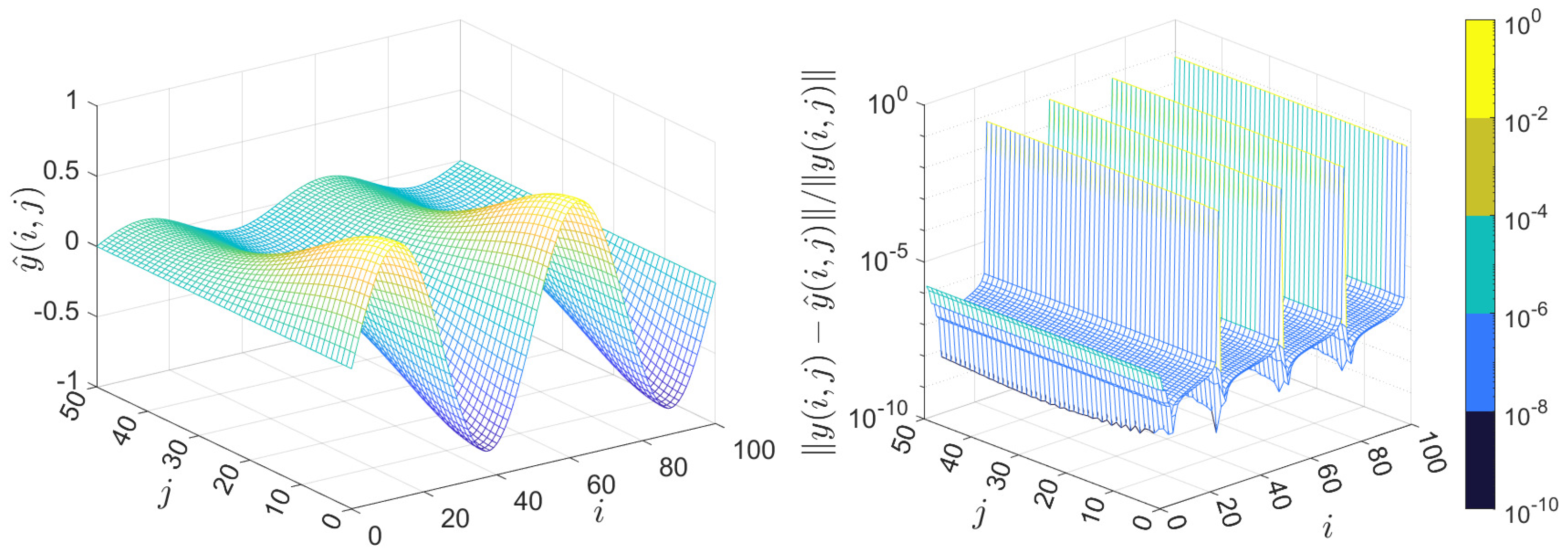
The transient responses $y(i,j)$ of the original system is shown in Figure 1 for the input $u(i,j)=sin\left(0.04\pi i\right)exp(cos(0.02\pi j\left)\right)$. We set $r_1=r_2=2$. Then, we can obtain the 4-order reduced two-dimensional discrete-time system (4) by Algorithm 1 and the reduced system matrices are given in the following

$${\widehat{A}}_1\left[\begin{array}{cc}{\widehat{A}}_1& {\widehat{B}}_1\\ {\widehat{A}}_2& {\widehat{B}}_2\\ \widehat{C}& \hfill \widehat{D}\end{array}\right]=\left[\begin{array}{ccccc}\hfill 0.8300& \hfill 0.0621& \hfill 0.3735& \hfill -0.0237& \hfill -5.2633\times {10}^{-5}\\ \hfill 0.0414& \hfill 0.2578& \hfill -0.2641& \hfill 0.2011& \hfill 1.0881\times {10}^{-5}\\ \hfill -0.0602& \hfill -0.4854& \hfill 0.4097& \hfill -0.4249& \hfill -1.9618\times {10}^{-5}\\ \hfill -0.0143& \hfill 0.1279& \hfill 0.4671& \hfill 0.5833& \hfill -4.5634\times {10}^{-6}\\ \hfill 0.0000& \hfill -0.0046& \hfill -0.0023& \hfill -0.0004& \hfill -4.4226\times {10}^{-9}\\ \hfill -0.0050& \hfill 0.5864& \hfill 0.3132& \hfill 0.0754& \hfill 3.9803\times {10}^{-7}\\ \hfill -0.0024& \hfill 0.2502& \hfill 0.1114& \hfill 0.0595& \hfill 2.1701\times {10}^{-7}\\ \hfill 0.0002& \hfill -0.0201& \hfill -0.0308& \hfill -0.0080& \hfill 2.0098\times {10}^{-7}\\ \hfill 0.0045& \hfill 0.0012& \hfill -0.0018& \hfill 0.0019& \hfill 0.3000\end{array}\right].$$

The transient responses of the 4-order reduced two-dimensional discrete-time system and the relative errors for the original system and its reduced system are given in Figure 2. Simulation results show that the relative errors are almost less than ${10}^{-7}$ and can reach to ${10}^{-10}$ at some times. However, at the points of $i=25,50,75,100$, the relative error increases significantly, rising to the order of ${10}^{-2}$. This spike is attributed to the fact that at these instants the true system outputs are vanishingly small (on the order of ${10}^{-7}$), which amplifies the computed relative error due to the denominator being close to zero. Additionally, without reconstructing the reduced system, we choose another input $u(i,j)=exp(sin(0.04\pi i\left)\right)exp(cos(0.02\pi j\left)\right)$, the transient responses and corresponding relative errors for the original system and reduced system are shown in Figure 3 and Figure 4. It is clearly observed that the output of the reduced system obtained by Algorithm 1 can well approximate the output of original two-dimensional discrete-time system for different input in this example.

Example 2: Here, we consider a two-dimensional discrete-time system of dimension n. The matrices $A_1\in {\mathbb{R}}^{n\times n}$ and $A_2\in {\mathbb{R}}^{n\times n}$ are given by

$$A_1=\left[\begin{array}{ccccc}0.01& 0.03& 0& & \\ 0.02& 0.01& 0.03& & \\ & \ddots & \ddots & \ddots & \\ & & 0.02& 0.01& 0.03\\ & & 0& 0.02& 0.01\end{array}\right],A_2=\left[\begin{array}{ccccc}0.07& 0.09& 0& & \\ 0.08& 0.07& 0.09& & \\ & \ddots & \ddots & \ddots & \\ & & 0.08& 0.07& 0.09\\ & & 0& 0.08& 0.07\end{array}\right].$$

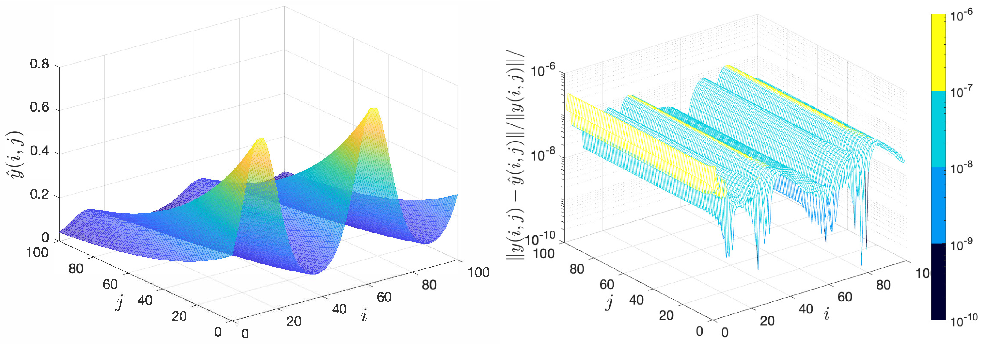
The matrices $B_1={[0.1,0.1,\cdots ,0.1]}^T$, $B_2=2B_1,C=B_1^T$, and $D=3.14$. For simulation, the order of the original system is set to be $n=5000$ and the input is $u(i,j)=-sin\left({\displaystyle \frac{i}{5}}\right){\left({\displaystyle \frac{30-j}{60}}\right)}^2$. We set $r_1=2,r_2=5$. Implementing the parallel input-independent and Krawtchouk-parameter-independent model reduction method in Algorithm 1, a 10-order reduced two-dimensional discrete-time system (4) is constructed. The transient response $y(i,j)$ of the original system is shown in Figure 5. Meanwhile, the transient response of the 10-order reduced two-dimensional discrete-time system and the relative errors for the original system and its reduced system are given in Figure 6. It is observed from the simulation results that the relative errors are almost less than ${10}^{-10}$ and can reach to ${10}^{-12}$ at some times, which indicates that the reduced two-dimensional discrete-time system obtained by Algorithm 1 has a good approximation to the original system.

To obtain the projection matrix V, an alternative method of computing the expansion coefficients $x_{k,l}(k=0,1,\cdots ,r_1-1,l=0,1,\cdots ,r_2-1)$ is to directly solve the large-scale linear algebraic Equation (8). In this example, the CPU times of constructing the projection matrix by Algorithm 1 and by directly solving the linear algebraic Equation (8) are 45.35 s and 102.17 s, respectively. This shows that the proposed parallel model reduction method is effective to speed up model reduction process of the 5000-order two-dimensional discrete-time system.

5. Conclusions

This paper discussed the model reduction via Krawtchouk moments for two-dimensional discrete-time systems. With the difference relation of Krawtchouk polynomials and the analytic identity theorem, the explicit formula related to the Krawtchouk moments of the state was given. To maintain the robustness of the reduced system for the input and Krawtchouk parameter, the subspace spanned by a sequence of input-independent and Krawtchouk-parameter-independent vectors was firstly derived, which was equivalent to the subspace spanned by the Krawtchouk moments for arbitrary input and arbitrary Krawtchouk parameter. Furthermore, instead of directly solving the large-scale linear equation, we designed a parallel strategy based on the equivalent transformation of block bi-diagonal Toeplitz matrices with bi-diagonal blocks to compute the basis of the projection subspace, which could speed up the construction of the reduced two-dimensional discrete-time systems. Then, we proposed the parallel input-independent and Krawtchouk-parameter-independent model reduction method based on the equivalent transformation and the block diagonalization technique. Further, we analyzed the Krawtchouk moment invariants of the proposed method. Numerical experiments showed that the reduced systems could approximate the original system and the proposed method could speed up the model reduction process on high performance computers. The proposed method also has several limitations. For two-dimensional systems not in FMLSS form (e.g., Roesser models), the resulting reduced system may fail to preserve the original state-space structure. Furthermore, the proposed method belongs to the time-domain method. Further exploration is needed into parallel model reduction methods in the frequency-domain for two-dimensional discrete-time systems.

References

1. Bechtold, T.; Schrag, G.; Feng, L.H. System-Level Modeling of MEMS; Wiley-VCH: Weinheim, Germany, 2013. [Google Scholar] [CrossRef]
2. Benner, P.; Cohen, A.; Ohlberger, M.; Willcox, K. Model Reduction and Approximation: Theory and Algorithms; SIAM: Philadelphia, PA, USA, 2017. [Google Scholar] [CrossRef]
3. Li, T.; Wang, B. Continuous-stage symplectic adapted exponential methods for charged-particle dynamics with arbitrary electromagnetic fields. Adv. Comput. Math. 2023, 49, 89. [Google Scholar] [CrossRef]
4. Li, M.; Nikan, O.; Qiu, W.; Xu, D. An efficient localized meshless collocation method for the two-dimensional Burgers-type equation arising in fluid turbulent flows. Eng. Anal. Bound. Elem. 2022, 144, 44–54. [Google Scholar] [CrossRef]
5. Urban, K.; Patera, A.T. An improved error bound for reduced basis approximation of linear parabolic problems. Math. Comput. 2013, 83, 1599–1615. [Google Scholar] [CrossRef]
6. Benner, P.; Breiten, T. Two-sided projection methods for nonlinear model order reduction. SIAM J. Sci. Comput. 2015, 37, B239–B260. [Google Scholar] [CrossRef]
7. Luo, Z.D.; Li, Y.J. A preserving precision mixed finite element dimensionality reduction method for unsaturated flow problem. Mathematics 2022, 10, 4391. [Google Scholar] [CrossRef]
8. Zimmermann, R.; Cheng, K. Randomized greedy magic point selection schemes for nonlinear model reduction. Adv. Comput. Math. 2024, 50, 81. [Google Scholar] [CrossRef]
9. Chellappa, S.; Feng, L.H.; Benner, P. Accurate error estimation for model reduction of nonlinear dynamical systems via data-enhanced error closure. Comput. Methods Appl. Mech. Eng. 2024, 420, 116712. [Google Scholar] [CrossRef]
10. Moore, B.C. Principal component analysis in linear systems: Controllability, observability, and model reduction. IEEE Trans. Autom. Control 1981, 26, 17–32. [Google Scholar] [CrossRef]
11. Pontes Duff, I.; Grundel, S.; Benner, P. New Gramians for switched linear systems: Reachability, observability, and model reduction. IEEE Trans. Autom. Control 2020, 65, 2526–2535. [Google Scholar] [CrossRef]
12. Benner, P.; Goyal, P. Balanced truncation for quadratic-bilinear control systems. Adv. Comput. Math. 2024, 50, 88. [Google Scholar] [CrossRef]
13. Jiang, S.; Cheng, Y.; Cheng, Y.; Huang, Y.Q. Generalized multiscale finite element method and balanced truncation for parameter-dependent parabolic problems. Mathematics 2023, 11, 4965. [Google Scholar] [CrossRef]
14. Tang, M.; Xiao, Z.H.; Zulfiqar, U. Structure-preserving low-rank model reduction for second-order time-delay systems. Mathematics 2025, 13, 474. [Google Scholar] [CrossRef]
15. Feng, L.H.; Benner, P. On error estimation for reduced-order modeling of linear non-parametric and parametric systems. ESAIM Math. Model. Numer. Anal. 2021, 55, 561–594. [Google Scholar] [CrossRef]
16. Jiang, L.J.; Ma, L.L. A hybrid model reduction method for stochastic parabolic optimal control problems. Comput. Methods Appl. Mech. Eng. 2020, 370, 113–244. [Google Scholar] [CrossRef]
17. Xu, K.L.; Jiang, Y.L.; Li, Z.; Li, L. Model reduction of discrete time-delay systems based on Charlier polynomials and high-order Krylov subspaces. Linear Algebra Appl. 2023, 661, 222–246. [Google Scholar] [CrossRef]
18. Yan, W.Y.; Lam, J. An approximate approach to H2 optimal model reduction. IEEE Trans. Autom. Control 1999, 44, 1341–1358. [Google Scholar] [CrossRef]
19. Jiang, Y.L.; Xu, K.L. Riemannian modified Polak-Ribière-Polyak conjugate gradient order reduced model by tensor techniques. SIAM J. Matrix Anal. Appl. 2020, 41, 432–463. [Google Scholar] [CrossRef]
20. Xu, K.L.; Jiang, Y.L. Riemannian geometric-nonlinear conjugate gradient model order reduction of linear port-Hamiltonian systems on finite frequency intervals. IEEE Trans. Autom. Control 2024, 69, 3317–3324. [Google Scholar] [CrossRef]
21. Borghi, A.; Breiten, T. H2 optimal rational approximation on general domains. Adv. Comput. Math. 2024, 50, 28. [Google Scholar] [CrossRef]
22. Xu, K.L.; Dong, L.H.; Wang, B.; Li, Z. Preserving-periodic Riemannian descent model reduction of linear discrete-time periodic systems with isometric vector transport on product manifolds. Appl. Math. Lett. 2025, 171, 109692. [Google Scholar] [CrossRef]
23. Rogers, E.; Galkowski, K.; Paszke, W.; Moore, K.L.; Bauer, P.H.; Hladowski, L.; Dabkowski, P. Multidimensional control systems: Case studies in design and evaluation. Multidimens. Syst. Signal Process. 2015, 26, 895–939. [Google Scholar] [CrossRef]
24. Barnett, A.; Wu, B.; Veerapaneni, S. Spectrally accurate quadratures for evaluation of layer potentials close to the boundary for the 2D Stokes and Laplace equations. SIAM J. Sci. Comput. 2015, 37, B519–B542. [Google Scholar] [CrossRef]
25. Roesser, R. A discrete state-space model for linear image processing. IEEE Trans. Autom. Control 1975, 20, 1–10. [Google Scholar] [CrossRef]
26. Fornasini, E.; Marchesini, G. Doubly-indexed dynamical systems: State-space models and structural properties. Math. Syst. Theory 1978, 12, 59–72. [Google Scholar] [CrossRef]
27. Fornasini, E.; Marchesini, G. State-space realization theory of two-dimensional filters. IEEE Trans. Autom. Control 1976, 21, 484–492. [Google Scholar] [CrossRef]
28. Lu, W.S.; Lee, E.B.; Zhang, Q.T. Balanced approximation of two-dimensional and delay-differential systems. Int. J. Control 1987, 46, 2199–2218. [Google Scholar] [CrossRef]
29. Imran, M.; Imran, M. Model order reduction framework for discrete-time systems with error bound via balanced structure. Int. J. Syst. Sci. 2022, 53, 3081–3094. [Google Scholar] [CrossRef]
30. Ghafoor, A.; Sreeram, V. Model reduction via limited frequency interval Gramians. IEEE Trans. Circuits Syst. Regul. Pap. 2008, 55, 2806–2812. [Google Scholar] [CrossRef]
31. Kumar, D.; Sreeram, V.; Du, X. Model reduction using parameterized limited frequency interval Gramians for 1-D and 2-D separable denominator discrete-time systems. IEEE Trans. Circuits Syst. Regul. Pap. 2018, 65, 2571–2580. [Google Scholar] [CrossRef]
32. Du, H.L.; Xie, L.H.; Soh, Y.C. H reduced-order approximation of 2-D digital filters. IEEE Trans. Circuits Syst. Fundam. Theory Appl. 2001, 48, 688–698. [Google Scholar] [CrossRef]
33. Gao, H.J.; Lam, J.; Wang, C.H.; Xu, S.Y. H model reduction for uncertain two-dimensional discrete systems. Optim. Control Appl. Methods 2005, 26, 199–227. [Google Scholar] [CrossRef]
34. Li, X.W.; Lam, J.; Cheung, K.C. Generalized H model reduction for stable two-dimensional discrete systems. Multidimens. Syst. Signal Process. 2016, 27, 359–382. [Google Scholar] [CrossRef]
35. Wang, X.L.; Jiang, Y.L. Model reduction of discrete-time bilinear systems by a Laguerre expansion technique. Appl. Math. Model. 2016, 40, 6650–6662. [Google Scholar] [CrossRef]
36. Samuel, E.R.; Knockaert, L.; Dhaene, T. Model order reduction of time-delay systems using a Laguerre expansion technique. IEEE Trans. Circuits Syst. Regul. Pap. 2014, 61, 1815–1823. [Google Scholar] [CrossRef]
37. Brugnano, L.; Frasca-Caccia, G.; Iavernaro, F.; Vespri, V. A new framework for polynomial approximation to differential equations. Adv. Comput. Math. 2022, 48, 76. [Google Scholar] [CrossRef]
38. Li, Z.; Jiang, Y.L. Parallel input-independent model order reduction for discrete-time parametric systems. IEEE Trans. Autom. Control 2023, 68, 4359–4366. [Google Scholar] [CrossRef]
39. Li, Z.; Jiang, Y.L. Parallel model order reduction methods based on structured matrix analysis for discrete-time systems with parametric uncertainty. J. Comput. Appl. Math. 2023, 426, 115088. [Google Scholar] [CrossRef]
40. Xu, K.L.; Li, Z.; Benner, P. Parametric interpolation model order reduction on Grassmann manifolds by parallelization. IEEE Trans. Circuits Syst. II Express Briefs 2025, 72, 198–202. [Google Scholar] [CrossRef]
41. Wang, Z.H.; Jiang, Y.L.; Xu, K.L. Reduced-order state-space models for two-dimensional discrete systems via bivariate discrete orthogonal polynomials. Math. Comput. Simul. 2023, 212, 441–456. [Google Scholar] [CrossRef]
42. Yap, P.T.; Paramesran, R.; Ong, S.H. Image analysis by Krawtchouk moments. IEEE Trans. Image Process. 2003, 12, 1367–1377. [Google Scholar] [CrossRef]
43. Beals, R.; Wong, R. Special Functions: A Graduate Text; Cambridge University Press: New York, NY, USA, 2010. [Google Scholar]
44. Du, C.L.; Xie, L.H. H Control and Filtering of Two-Dimensional Systems; Springer: Berlin/Heidelberg, Germany, 2002. [Google Scholar] [CrossRef]
Figure 1. Transient responses of the 12-order two-dimensional discrete-time system, u ( i , j ) = sin ( 0.04 π i ) exp ( cos ( 0.02 π j ) ) .
Mathematics 13 02565 g001
Figure 2. Transient responses of the 4-order reduced two-dimensional discrete-time system and the relative output errors, u ( i , j ) = sin ( 0.04 π i ) exp ( cos ( 0.02 π j ) ) , r 1 = r 2 = 2 .
Mathematics 13 02565 g002
Figure 3. Transient responses of the 12-order two-dimensional discrete-time system, u ( i , j ) = exp ( sin ( 0.04 π i ) ) exp ( cos ( 0.02 π j ) ) .
Mathematics 13 02565 g003
Figure 4. Transient responses of the 4-order reduced two-dimensional discrete-time system and the relative output errors, u ( i , j ) = exp ( sin ( 0.04 π i ) ) exp ( cos ( 0.02 π j ) ) , r 1 = r 2 = 2 .
Mathematics 13 02565 g004
Figure 5. Transient responses of the 5000-order two-dimensional discrete-time system, u ( i , j ) = sin ( i 5 ) ( 30 j 60 ) 2 .
Mathematics 13 02565 g005
Figure 6. Transient responses of the 10-order reduced two-dimensional discrete-time system and the relative output errors, u ( i , j ) = sin ( i 5 ) ( 30 j 60 ) 2 , r 1 = 2 , r 2 = 5 .
Mathematics 13 02565 g006
Disclaimer/Publisher’s Note: The statements, opinions and data contained in all publications are solely those of the individual author(s) and contributor(s) and not of MDPI and/or the editor(s). MDPI and/or the editor(s) disclaim responsibility for any injury to people or property resulting from any ideas, methods, instructions or products referred to in the content.