A Clustering Algorithm for Large Datasets Based on Detection of Density Variations

Abstract

Clustering algorithms help handle unlabeled datasets. In large datasets, density-based clustering algorithms effectively capture the intricate structures and varied distributions that these datasets often exhibit. However, while these algorithms can adapt to large datasets by building clusters with arbitrary shapes by identifying low-density regions, they usually struggle to identify density variations. This paper proposes a Variable DEnsity Clustering Algorithm for Large datasets (VDECAL) to address this limitation. VDECAL introduces a large-dataset partitioning strategy that allows working with manageable subsets and prevents workload imbalance. Within each partition, relevant objects subsets characterized by attributes such as density, position, and overlap ratio are computed to identify both low-density regions and density variations, thereby facilitating the building of the clusters. Extensive experiments on diverse datasets show that VDECAL effectively detects density variations, improving clustering quality and runtime performance compared to state-of-the-art DBSCAN-based algorithms developed for clustering large datasets.

1. Introduction

Clustering aims to divide datasets into groups called clusters. The objects of a cluster must be similar and different from those of other clusters [1,2,3,4,5]. The clustering problem has appeared in various disciplines and contexts, reflecting the broad applicability of this technique, probably due to one of its main characteristic: the ability to deal with unlabeled data [6,7,8,9,10]. The broad applicability of clustering has motivated the development of several algorithms adapted to different types of datasets, such as stream datasets [11], categorical or numerical datasets [12], high dimensional datasets [13,14], point clouds [15], large datasets [16], and others. Recently, due to the increasing amount of data generated by current information systems, the development of clustering algorithms capable of processing large datasets has become an important research topic [17,18,19].

Clustering large datasets presents several challenges, including the development of efficient techniques to handle them effectively [20]. However, this is not the only challenge to consider. Clustering large datasets should also address the diversity in the data, which follows unknown distributions [21,22]. Therefore, several clustering algorithms for large datasets employ approaches that allow the construction of clusters with arbitrary shapes, i.e., that do not necessarily follow a Gaussian distribution [23].

The density-based clustering approach builds clusters by establishing connectivity relationships between objects in the dataset and identifying regions with at least a predetermined number of points. This approach creates clusters with arbitrary shapes and allows for dealing with noisy data [24,25,26]. However, due to the inherent properties of the density-based approach, it requires a high number of comparisons between objects in the dataset [27]. For this reason, density-based clustering algorithms must use scalable approaches such as sampling, data projection, parallelism, and distributed techniques to process large datasets [28,29,30,31].

In addition to the use of scalable approaches, techniques for building clusters rapidly and reducing the number of comparisons between the elements in the dataset without losing the advantages of density-based clustering, are required. The most common way for building clusters with arbitrary shapes is identifying high-density regions separated by low-density regions.

However, a practical issue in large datasets arises when clusters are not separated by low-density regions, but by density variations in regions with approximately homogeneous densities [32,33]. Building clusters using information about density variations is helpful in problems such as segmenting objects in medical images [34,35,36,37] or reconstructing objects from point clouds generated by sensors [38,39,40]. These problems have in common the detection of clusters of interest by identifying changes in the distribution of objects belonging to the dataset.

Building clusters using density variations has been studied for small datasets but has not been addressed for large datasets [32,33,41,42,43]. For this reason, this paper introduces a clustering algorithm that builds clusters with arbitrary shapes in large datasets called Variable DEnsity Clustering Algorithm for Large datasets (VDECAL). VDECAL identifies density variations to build clusters, aiming to improve clustering quality while processing large datasets. Our experiments on synthetic and standard public datasets, commonly used to assess clustering algorithms, demonstrated that the proposed algorithm, VDECAL, has the best compromise between runtime and quality.

Our contributions include the following:

• A new large-dataset partitioning strategy that allows working with manageable subsets and prevents workload imbalance. This strategy could be used in other large-dataset clustering algorithms.
• A new strategy to build clusters by identifying density variations and low-density regions in large datasets.
• Based on the above, we also contribute with the Variable DEnsity Clustering Algorithm for Large datasets VDECAL.

The rest of this work is organized as follows. Section 2 presents the related work. Section 3 introduces the proposed algorithm. Section 4 shows an experimental evaluation of the proposed algorithm. Section 5 presents the conclusions and future work.

2. Related Work

The increasing amount of data generated by current information systems requires the development of algorithms capable of processing large amounts of data by overcoming the challenges that large datasets present, such as volume, variety, and velocity [44].

To address the growing amount of information, distributed architectures (such as Apache Spark and Hadoop) have been designed [23,27,45,46,47]. For this reason, most recent density-based algorithms are designed to be scalable for these architectures, employing techniques like partitioning, sampling, and others to handle large datasets [28].

Numerous algorithms address clustering in large datasets. This work focuses on density-based methods, as they manage challenges common in large datasets, such as noise and arbitrary cluster shapes, among others. These methods are particularly well-suited for capturing the complex structures and variability found in such data. The analyzed methods are presented below.

DBSCAN [48] is the cornerstone of density-based clustering, so it is not surprising that algorithms for processing large datasets are based on it. SDBSCAN [30] was proposed in 2016 to have a comparable version of DBSCAN for large datasets. To do this, SDBSCAN uses three phases: Partitioning, Processing, and Clustering. First, the large dataset is randomly partitioned; second, each partition is analyzed with DBSCAN; and third, the resulting clusters are grouped based on the distance between their centroids. Like SDBSCAN, other algorithms use the phases of partitioning, processing, and clustering to process large datasets by executing most of the process in parallel to reduce the runtime. DBSCAN-PSM [49] improves the partitioning process and the parallel processing using a k-d Tree, which reduces the number of I/O operations. In addition, the clustering process was also enhanced by reviewing the proximity of the local clusters’ borders.

RNN-DBSCAN algorithm [50], proposed in 2018, builds clusters using nearest neighbors approach to identify density variations. For this, the k-nearest neighbors for every object are calculated and the distance between them are compared to determine if they can be in the same cluster. A k-d tree is employed to speed up the search of the k-nearest neighbors. The algorithm does not mention that it processes large datasets.

Finally, RS-DBSCAN [51], proposed in 2024, is an algorithm designed to process large datasets, built on top of the RNN-DBSCAN algorithm. RS-DBSCAN partitions the dataset, and every partition is processed independently with RNN-DBSCAN. From the local clusters, a set of representative objects are selected. Then, RNN-DBSCAN is applied to classify all representative objects globally. Finally, the dataset is clustered using these representative objects. This process is faster than RNN-DBSCAN; however, it cannot detect density variations, as opposed to RNN-DBSCAN.

Another widely used technique in density-based algorithms for processing large datasets is the identification of density peaks (high-density regions), which can quickly obtain the cluster centers by drawing the decision diagram by using the calculation of local density and relative distance. Below are some algorithms that build clusters based on density peaks [52].

FastDPeak [53], proposed in 2020, is an algorithm built on top of the DPeak algorithm and designed to process large datasets. FastDPeak builds clusters by identifying the dataset’s density peaks and also uses a three-phases partitioning process. The partitioning phase is performed using the kNN algorithm. The processing phase picks up the ideas of the DPeak algorithm applied to the partitions created in the first phase. The results are grouped by creating a DPeak tree that contains information about the density peaks and the objects associated with these peaks. Using the DPeak tree as a tool, the clusters are built.

The KDBSCAN algorithm [54], proposed in 2021, is also a three-phase partitioning algorithm. In the first phase, the dataset is partitioned using the K-Means++ algorithm [55], using a reduced number of iterations without achieving convergence; this algorithm works in the same way as K-Means, with the difference that the selection of initial centroids is not random. In the second phase, KDBSCAN, like S-DBSCAN or DBSCAN-PSM algorithm, uses DBSCAN to process the partitions. In the clustering phase, the "close" clusters are identified by analyzing the distances between their centroids, and then those close clusters are grouped again with DBSCAN.

KNN-BLOCK DBSCAN [56], proposed in 2021, improves the quality of DBSCAN and speeds up the processing of large datasets. This algorithm merges the partitioning and processing phases in a version of the KNN algorithm called FLANN. In this phase, three groups of objects are created: core blocks, non-core blocks, and noise. In the merging phase, clusters are formed by connecting core blocks when they are densely reachable. Non-core blocks near clusters are merged to form clusters. Noise and non-core blocks that are not near a cluster are discarded. KNN-BLOCK DBSCAN builds clusters based on identifying density peaks; however, this approach assumes that the cluster center has a higher density than the surroundings, in addition to the fact that there is a low-density region between the clusters, as Huan Yan stated in their paper on the ANN-DPC algorithm [57], which explores this approach on smaller datasets.

In 2023, the GB-DP algorithm [58] was introduced as a three-phase clustering algorithm based on detecting density peaks. First, GB-DP partitions the dataset using K-Means; the clusters built are called granular balls. It then uses the characteristics of these granular balls, such as density and distance, to build a decision graph for identifying density peaks. In the last phase, granular balls and the points they represent are assigned to their nearest peaks, allowing for the build of clusters. This way of building clusters is partition-based rather than density-based.

Though the mentioned algorithms employ partitioning to create dataset sections, it is important to note that partitioning is not the only option. Other algorithms select a dataset sample to create a preliminary version of the clusters. This reduces runtime by performing operations with a higher load on the selected sample. Usually, after processing the sample, these algorithms extrapolate the results to the rest of the dataset.

For example, in 2019, DBSCAN++ [59] was proposed as an alternative to using DBSCAN on large datasets by following sample selection. DBSCAN++ selects a random subset of the dataset that is large enough to be meaningful but small enough to be processed by DBSCAN. DBSCAN processes the selected subset to build the clusters. The rest of the dataset is clustered by assigning each element to the nearest cluster. This algorithm reduces the runtime and maintains the quality of DBSCAN as long as the selected subset is representative of the dataset.

Improved K-Means [60], proposed in 2020, has emerged as an alternative that combines partition-based algorithm techniques with density-based algorithm techniques. This can be used to build arbitrarily shaped clusters in large datasets. Improved K-Means, like DBSCAN++, selects a sample from the dataset and uses it to identify reference objects that represent the highest density regions. Clusters are formed using these reference objects. The remaining objects are assigned to the closest cluster, using the reference objects and a distance function.

The OP-DBSCAN algorithm [61], proposed in 2022, also uses sample selection to analyze large datasets. OP-DBSCAN selects a set of objects from the dataset close to each other; this set is called the operational dataset. Then, the operational dataset is clustered using DBSCAN. Next, OP-DBSCAN finds the boundaries of the previously computed clusters. Finally, OP-DBSCAN computes the objects closest to the previously determined boundaries; these objects now form the operational dataset. This process is repeated until the entire dataset is analyzed, constantly updating the operational dataset. Although the sample is more controlled and computed multiple times, the goal of selecting a sample is to reduce the number of comparisons between objects, thus reducing the runtime.

UP-DPC [62], proposed in 2024, is also a sampling-based framework for cluster building, operating through four steps. It begins by sampling a random subset of the dataset and identifying local density peaks through partitioning. Then, it constructs a similarity graph between these peaks and the samples. The graph is refined to improve accuracy. Finally, the density of local peaks is calculated and the significant ones are selected as initial cluster labels, thus clustering all objects in the dataset. Although UP-DPC uses density-based techniques to identify density peaks, clusters are built by assigning objects to the nearest peak, being a partitional technique which limits the type of clusters built.

As seen in the above works, current density-based clustering algorithms for large datasets aim to identify clusters by detecting high-density regions separated by low-density boundaries. This approach relies on well-defined, low-density separation zones, which can limit the effectiveness of clustering algorithms like SDBSCAN and KDBSCAN. Moreover, traditional partitioning methods, such as random partitioning or K-Means, may result in imbalanced partitions. Thus, an opportunity area for research is the development of clustering algorithms for large datasets that enable the identification of cluster boundaries via low-density areas or density fluctuations and by utilizing balanced partitioning to ensure equitable workload distribution when clustering large datasets.

3. Proposed Algorithm

This section introduces the proposed Variable DEnsity Clustering Algorithm for Large datasets (VDECAL). The main goal of VDECAL is to create clusters with arbitrary shapes in large datasets using density-based techniques. Unlike previously studied clustering algorithms that focus on identifying low-density regions that can be used as boundaries for clustering, VDECAL also identifies variations in the density of nearby regions, allowing the separation of clusters with density variations. This approach aims to improve the clustering quality of clustering without increasing the runtime in large datasets.

3.1. Preliminary Definitions

Density-based clustering is an approach in which clusters are defined as sets of objects distributed in the data space in a continuous region with high object density (with many objects). Regions with few objects are called low-density regions. In this way, clusters are separated by low-density regions. Objects in low-density regions are considered as noise [25].

One way to quantify the density of a region is to calculate the number of objects near a reference point. The set of objects near a reference point is called the neighborhood of the reference point. To determine if two objects are nearby, a parameter $ϵ$ indicates the maximum distance between two objects to be considered close [63]; in this sense, a $ϵ$-neighborhood is defined as follows.

Definition 1.

ϵ-Neighborhood. Consider a set of objects $O=\{o_1,o_2,\dots ,o_n\}$ in a k-dimensional space ${\mathbb{R}}^k$, a distance function $Distance:{\mathbb{R}}^k\times {\mathbb{R}}^k\to \mathbb{R}$, and a distance threshold $ϵ\in {\mathbb{R}}^{+}$. The ϵ-neighborhood of an object x, denoted by $N_{ϵ}\left(x\right)$, is as follows:

$$N_{ϵ}\left(x\right)=\{o\in O|Distance(x,o)\le ϵ\}$$

(1)

A second parameter, $minPts$, indicates whether the neighborhood of an object is dense enough to be considered a high-density region or, on the contrary, whether it is a low-density region. An object that exceeds the specified density ($minPts$) is called a core object [63].

Definition 2.

Core object. Consider a set of objects $O=\{o_1,o_2,\dots ,o_n\}$ in a k-dimensional space ${\mathbb{R}}^k$, a distance threshold $ϵ\in {\mathbb{R}}^{+}$ and a minimum density $minPts\in {\mathbb{Z}}^{+}$. An object $o_i\in O$ is called a core object if $|N_{ϵ}\left(o_i\right)|\ge minPts$.

Identifying core objects in a dataset and connecting them by their common objects is the most commonly used technique by density-based algorithms to build clusters. However, this requires comparisons among multiple objects. In large datasets, this process can be time-consuming. To assess this problem, our proposed algorithm reduces the number of calculations by using only selected reference points to determine the density of a region. For this purpose, the concept of a relevant object subset was introduced.

Definition 3.

Relevant object subset. Consider a set of objects $O=\{o_1,o_2,\dots ,o_n\}$ in a k-dimensional space ${\mathbb{R}}^k$, a distance threshold $ϵ\in {\mathbb{R}}^{+}$, and an object $c\in {\mathbb{R}}^k$. A relevant object subset R in the set O is represented as a 3-tuple $(M,{ϵ}_R,c)$, where $c\in {\mathbb{R}}^k$ is the centroid of the relevant object subset, ${ϵ}_R\in {\mathbb{R}}^{+}$ defines the size of the neighborhood, and $M\subset O$ contains objects within the relevant object subset such that $M=N_{{ϵ}_R}\left(c\right)$.

Therefore, the density of a relevant object subset is defined as follows.

Definition 4.

Density of a relevant object subset. Consider a relevant object subset $R=(M,{ϵ}_R,c)$. The density of R, denoted as $\rho \left(R\right)$, is the number of objects in the set M.

$$\rho \left(R\right)=\left|M\right|$$

(2)

Relevant object subsets with a density less than $minPts$ represent low-density regions. The drawback of using only low-density regions for cluster building is that some datasets may lack defined low-density regions. In such cases, clusters could be identified by assessing density variations between neighboring relevant object subsets.

Figure 1a depicts a dataset where a low-density region separates two clusters. In this scenario, it is possible to use the parameters $ϵ$ and $minPts$ to define the low-density region between clusters and separate them. Figure 1b represents a dataset where no low-density region exists between clusters. There only exists a density variation.

3.2. Variable DEnsity Clustering Algorithm for Large Datasets (VDECAL)

VDECAL aims to build clusters with arbitrary shapes in large datasets, and it is divided into three stages: dataset partitioning, finding relevant object subsets, and clustering relevant object subsets. In the first stage, dataset partitioning, the dataset is divided into independent segments, which reduces the number of comparisons between objects. In the next stage, finding relevant object subsets, VDECAL computes relevant object subsets for each partition. Finally, in the last stage, clustering relevant object subsets, the characteristics of the relevant object subsets, such as proximity, density, and their associated objects, are used to build the resulting clusters.

3.2.1. Dataset Partitioning

In the literature, a common approach for partitioning is using K-Means++. Without reaching the convergence for partitioning, the dataset produces good results because it creates partitions of nearby objects. However, unbalanced subsets may occur. When the subsets are unbalanced, the workload accumulates in the subsets with more objects. In extreme cases, this could lead to the partitioning stage becoming useless. To assess imbalanced subsets, we propose a recursive partitioning method.

The proposed dataset partitioning splits the dataset using K-Means++ (without reaching convergence) into two subsets. If the size of some of the resulting subsets exceeds the partition size t, it is partitioned again using K-Means++. This process continues until all partitions have less objects than t. This method is described in Algorithm 1.

Algorithm 1 Algorithm for dataset partitioning.

procedure Partition(Dataset D, partition size t)      Initialize an empty list $partitionList$      if number of elements in $D>t$ then          Divide D into two parts $D_1$ and $D_2$ using the K-Means++ algorithm.          $subset{s}_1$ = Partition ($D_1$, t)          $subset{s}_2$ = Partition ($D_2$, t)          Merge $subset{s}_1$ and $subset{s}_2$ into $partitionList$.      else          Add D to $partitionList$ as a partition.      end if      return $partitionList$ end procedure

Figure 2 compares two methods for dividing a dataset: K-Means++ and our proposed approach. In K-Means++ configured to create four partitions (see Figure 2a), we observe that most of the dataset’s objects are concentrated in a single partition. This leads to an uneven distribution of objects across partitions, causing workload imbalance. In contrast, our method (see Figure 2b), with $t=2000$, creates two partitions in the same region, effectively distributing the workload more evenly.

3.2.2. Finding Relevant Object Subsets

This stage aims to find a set of relevant object subsets for each partition P generated in the first stage, using a distance threshold $ϵ$. These relevant object subsets are computed according to Definition 3, which states that a relevant object subset is a 3-tuple $R=(M,{ϵ}_R,c)$: the set M contains the objects represented by the relevant object subset. The distance ${ϵ}_R$ defines the size of the neighborhood that the relevant object subset R covers. Finally, c is the centroid of the relevant object subset R.

All objects in a partition P are analyzed to calculate the relevant object subsets. For each object, o in P, that has not been previously added to a relevant object subset, a new relevant object subset R is created from o. All objects p in P whose distance to o is less than or equal to $ϵ$ are selected, whether or not they have been added to another relevant object subset, to create a relevant object subset $R=(M,{ϵ}_R,c)$ with o. These selected objects, including o, form the set M. From M, the centroid c is calculated as the mean of all the objects in M, and ${ϵ}_R$ is defined as the distance from c to the farthest object in M. This process ends when all objects in P have been added to one or more relevant object subsets. This process is shown in Algorithm 2.

Algorithm 2 Algorithm for finding relevant object subsets in a partition.

procedure FindRelevantObjectSubsets(partition P, distance threshold $ϵ$)      Initialize an empty list $relevantObjectSubsets$      for each object o in P do           if o is not visited then              $M=\{p\in P$ such that $Distance(o,p)\le ϵ\}$              $c=$ centroid of M              ${ϵ}_R={max}_{i=1,\dots ,\left|M\right|}Distance(c,m_i)$              Create a new relevant object subset R = ($M,{ϵ}_R,c)$              Add R to $relevantObjectSubsetSubsets$              Mark each object in M and o as visited           end if      end for      return $relevantObjectSubsets$ end procedure

3.2.3. Clustering Relevant Object Subsets

The final stage of the VDECAL algorithm involves building clusters using the relevant object subsets identified in the previous stage. This process relies on identifying overlaps and density variations among these relevant object subsets. Building clusters from the relevant object subsets begins by discarding those not meeting the minimum density requirement set by the parameter $minPts$ (see Definition 4).

The next step is to identify the relevant object subsets in the same cluster. Each pair of relevant object subsets is examined to determine if their neighborhoods overlap and have similar densities. The criterion for determining when two relevant object subsets are close enough to share neighborhoods, meaning they overlap, is given in Definition 5.

Definition 5.

Overlap of relevant object subsets. Consider two relevant object subsets $R_1=(M_1,{ϵ}_1,c_1)$ and $R_2=(M_2,{ϵ}_2,c_2)$ and a distance function $Distance:{\mathbb{R}}^k\times {\mathbb{R}}^k\to \mathbb{R}$. $R_1$ has an overlap with $R_2$ if the following condition is fulfilled.

$$Distance(c_1,c_2)\le ({ϵ}_1+{ϵ}_2)$$

(3)

To determine if there is a density variation between two relevant object subsets, $R_1$ and $R_2$, we first need to identify their neighboring relevant object subsets. The neighboring relevant object subsets of $R_1$, denoted by $\Omega \left(R_1\right)$, are those that overlap with $R_1$, and similarly, the neighboring relevant object subsets of $R_2$, denoted by $\Omega \left(R_2\right)$, are those that overlap with $R_2$ (Definition 5). Once these neighbors are identified, the density of each neighboring relevant object subset $\rho \left(R\right)$ is obtained (Definition 4). Then, we calculate the mean ($\overline{x}$) and standard deviation ($\sigma$) of the densities for the neighboring relevant object subsets of $R_1$ and $R_2$, obtaining the mean and standard deviation of the densities for $R_1$ and those for $R_2$. Next, we calculate the Z-score of $R_1$ relative to the neighbors of $R_2$ and $R_2$ relative to the neighbors of $R_1$ according to Definition 6.

Definition 6.

Z-score of $R_2$ relative to the neighbors of $R_1$. Let $R_1=(M_1,{ϵ}_1,c_1)$ and $R_2=(M_2,{ϵ}_2,c_2)$ be two relevant object subsets. The Z-score of $R_2$ relative to the neighbors of $R_1$ is defined as:

$$Z(R_2,R_1)={\displaystyle \frac{\rho \left(R_2\right)-{\overline{x}}_{\Omega \left(\rho \left(R_1\right)\right)}}{{\sigma }_{\Omega \left(\rho \left(R_1\right)\right)}}}$$

(4)

where $\rho \left(R_2\right)$ is the density of $R_2$ (see Definition 4), ${\overline{x}}_{\Omega \left(\rho \left(R_1\right)\right)}$ is the mean of the densities of the neighboring relevant object subsets of $R_1$, and ${\sigma }_{R_1}$ is the standard deviation of the densities of the neighboring relevant object subsets of $R_1$.

The following definition states when there is a density variation between two relevant object subsets.

Definition 7.

Density variation between two relevant object subsets. Consider two relevant object subsets $R_1=(M_1,{ϵ}_1,c_1)$ and $R_2=(M_2,{ϵ}_2,c_2)$, and a density variation threshold $\delta \in {\mathbb{R}}^{+}$. There exists a density variation between $R_1$ and $R_2$ if any of the following conditions is fulfilled.

$$\delta \le |Z(R_1,R_2)|or\delta \le |Z(R_2,R_1)|.$$

Parameter $\delta$ should be determined in terms of the absolute Z-score. Z-score shows how many standard deviations a relevant object subset is from the mean of its neighbors. As a result, the values for $\delta$ must be between 0 and 4, since according to Shiffler [64] there are no absolute Z-scores that exceed 4 in limited sets.

VDECAL constructs an adjacency matrix using information about relevant object subsets that can be clustered using the overlap and density properties. In each cell $i,j$, the adjacency matrix contains a 1 if the relevant object subsets $R_i$ and $R_j$ overlaps and do not have a density variation, and 0 otherwise. With this adjacency matrix, the final clusters can be built by computing the connected components [65] (p. 552). Finally, each object in the dataset is assigned to a cluster by identifying the relevant object subsets to which it belongs. If it only belongs to relevant object subsets within the same cluster, it is assigned to that cluster. The object is labeled as noise if it belongs to a relevant object subset that was discarded because it did not meet the $minPts$ threshold. Finally, if the object belongs to relevant object subsets in different clusters, it will be assigned to the cluster with the relevant object subset with the closest centroid($c_R$).

In summary, given a large dataset, the proposed algorithm begins by partitioning the input dataset, employing K-Means++ as explained in Section 3.2.1. On each partition, the relevant object subsets are computed according to Section 3.2.2, which includes calculating the objects they represent, their centroids, and their neighborhood sizes. Next, we label the objects included in low-density relevant object subsets as noise. In Section 3.2.3, we construct a graph to connect the relevant object subsets after calculating them for all the partitions. The edges are made between overlapping relevant object subsets (Definition 5) that have similar density levels (Definition 7). The clusters emerge from building the connected components on the graph. In the final step, we assign each object not labeled as noise to a cluster by identifying the relevant object subsets to which it belongs. This clustering process is summarized in Algorithm 3.

Algorithm 3 VDECAL algorithm.

procedure VDECAL($D,ϵ,\mathrm{minPts},\delta ,t$)      Create a partition list of the dataset D using Partition($D,t$).      for each partition P in the partition list do           Find relevant object subsets in P using FindRelevantObjectSubsets$(P,ϵ)$.           Mark objects in relevant object subsets with density less than $minPts$ as noise.      end for      Build a graph connecting relevant object subsets           with overlapping neighborhoods (Definition 5) and           density variation below $\delta$ (Definition 7).      Extract clusters as connected components of the graph.      for each object o in D not marked as noise do           Assign o to the cluster of the nearest relevant object subset in its $ϵ$-neighborhood.      end for end procedure

3.3. Effect of the t, $ϵ$, $minPts$, and $\delta$ Parameters

VDECAL has four parameters: partition size (t), neighborhood size ($ϵ$), minimum number of objects per relevant object subset ($minPts$), and density variation threshold ($\delta$). The parameter t sets the partition size. Small values for this parameter generate more and smaller partitions, producing subsets with insufficient information to build relevant object subsets. Conversely, higher values generate fewer and larger partitions, which slow down the construction of relevant object subsets. According to our experiments, shown later, taking 20% of the dataset provides good results.

High values for $ϵ$ produce fewer relevant object subsets and reduce VDECAL’s runtime but may blur cluster boundaries. Low values for $ϵ$ improve boundary detection but increase VDECAL’s runtime. The parameter $minPts$ allows VDECAL to discard relevant object subsets in low-density regions, thereby differentiating high-density areas by separating relevant object subsets with overlapping neighborhoods. Regarding $ϵ$ and $minPts$, given that they are highly data-dependent, it is difficult to recommend a value for them.

VDECAL uses the Z-score to determine density variations. Shiffler [64] stated that absolute Z-scores cannot exceed 4, so $\delta$ must range from 0 to 4. VDECAL does not detect density variations when $\delta =4$; however, as $\delta$ decreases, more density variations are identified. When $\delta =0$, every relevant object subset constitutes a cluster. From our experiments, shown later, fixing delta around 2.5 produces good results.

Setting values for the VDECAL’s parameters, as with other density-based clustering algorithms, remains a challenging issue due to its dependence on the specific characteristics of the dataset.

3.4. Time Complexity

For this analysis, we considered the three stages of the algorithm: partitioning, processing, and clustering. The partitioning stage involves recursively dividing the dataset into two partitions using K-Means++ until each partition contains a maximum of t points. The time complexity of K-Means++ is $O\left(2in\right)$, where 2 is the number of partitions, i represents the iterations to determine the centroids, and n represents the number of reviewed objects. The worst-case scenario occurs when K-Means++ separates only one object in each iteration. We intentionally keep i small because achieving full convergence is not necessary for our purposes. In this context, the time complexity for the first stage can be expressed as:

$$\begin{array}{cc}\hfill \sum _{x=0}^{n-t}2i(n-x)& =-i(t-n-1)(t+n)\hfill \\ \hfill & =i{n}^2+in-i{t}^2+it\hfill \end{array}$$

where t represents the maximum number of elements per partition. By ignoring the constant terms, we can focus on the dominant term, which in this case is $n^2$, indicating a quadratic complexity of $O\left(n^2\right)$ for the first stage.

For the processing stage, the worst case occurs when a relevant object subset is built for every object in the partition. Since creating relevant object subsets involves comparing the objects in the partition against the relevant object subsets found, the number of operations in the worst case is expressed as $O\left(t^2(n/t)\right)=O\left(tn\right)$, where t is the maximum number of objects in the partition and $n/t$ is the number of partitions found. However, since t is a constant, the complexity of this stage is $O\left(n\right)$.

Finally, the clustering stage analyzes all the relevant object subsets found in the partitions. To determine if two relevant object subsets can be merged, they need to be compared against the rest, requiring $r^2$ operations, where r is the number of relevant objects subsets. The worst case is when the number of relevant object subsets found is equal to the number of objects in the dataset, resulting in $O\left(n^2\right)$. To build the clusters, connected components need to be built, which is $O\left(\right(n+m)logn)$ ([66], ch. 25, p. 24), where m is the number of overlapping relevant object subsets. Therefore, for this stage the complexity is $O(n^2+((n+m)logn)=O\left(n^2\right)$ in the worst case.

Given that the partitioning stage is $O\left(n^2\right)$, the processing stage is $O\left(n\right)$ and the clustering stage is $O\left(n^2\right)$. Considering the dominant terms in each stage, the time complexity of the VDECAL algorithm is $O\left(n^2\right)$. This complexity is similar to that of other recent density-based algorithms when their worst-case behavior is also considered [51,54]. For this reason, we include a runtime evaluation to empirically assess its performance.

4. Experiments and Results

This section presents the experiments conducted to assess the performance of the proposed algorithm, VDECAL. The experiments encompass an analysis of the algorithm’s stability and convergence, as well as its quality, runtime, and scalability regarding the number of objects and dimensions.

We include a comparison against state-of-the-art density-based clustering algorithms. The selected algorithms include DBSCAN [48], which serves as the reference algorithm for density-based clustering; IKMEANS [60], an algorithm for large datasets that performs sampling on the dataset; KDBSCAN [54], which is an improvement of DBSCAN for large datasets based on dataset partitioning; KNN-BLOCK DBSCAN [56], another algorithm for large datasets that identifies objects called core blocks; RNNDBSCAN [50], an algorithm that detects density variations; and RSDBSCAN [51], a recent enhancement of RNNDBSCAN designed for large datasets.

To allow a fair comparison with the state-of-the-art clustering algorithms, we implemented each algorithm in Python (latest v. 3.13.5), using the same data structures for input/output processing for all algorithms. Experiments were conducted on a computer with two Intel Xeon E5-2620 at 2.40 GHz processors, 256 GB RAM, and Linux Ubuntu 22.

4.1. Stability and Convergence

Clustering algorithms often involve randomness, which can impact their results and lead to variations across different runs. VDECAL introduces randomness during the dataset partitioning stage by employing K-Means++, which selects random objects as initial centroids for each partition. This experiment aims to evaluate the stability and convergence of VDECAL. To assess these characteristics, we performed multiple runs of the algorithm using different random seeds and the corresponding object processing orders generated by these seeds, while keeping all other parameters constant.

For this experiment, we used the Compound dataset from Tomas Barton’s repository [67]. Compound is widely used to assess density-based clustering algorithms, as it contains clusters with arbitrary shapes, noise, concentric clusters, clusters with varying densities, and clusters with close boundaries. The parameters used were $t=200$ (resulting in two partitions), $ϵ=1.5$, $minPts=3$, and $\delta =3$. These values allow VDECAL to build the known clusters in the Compound dataset.

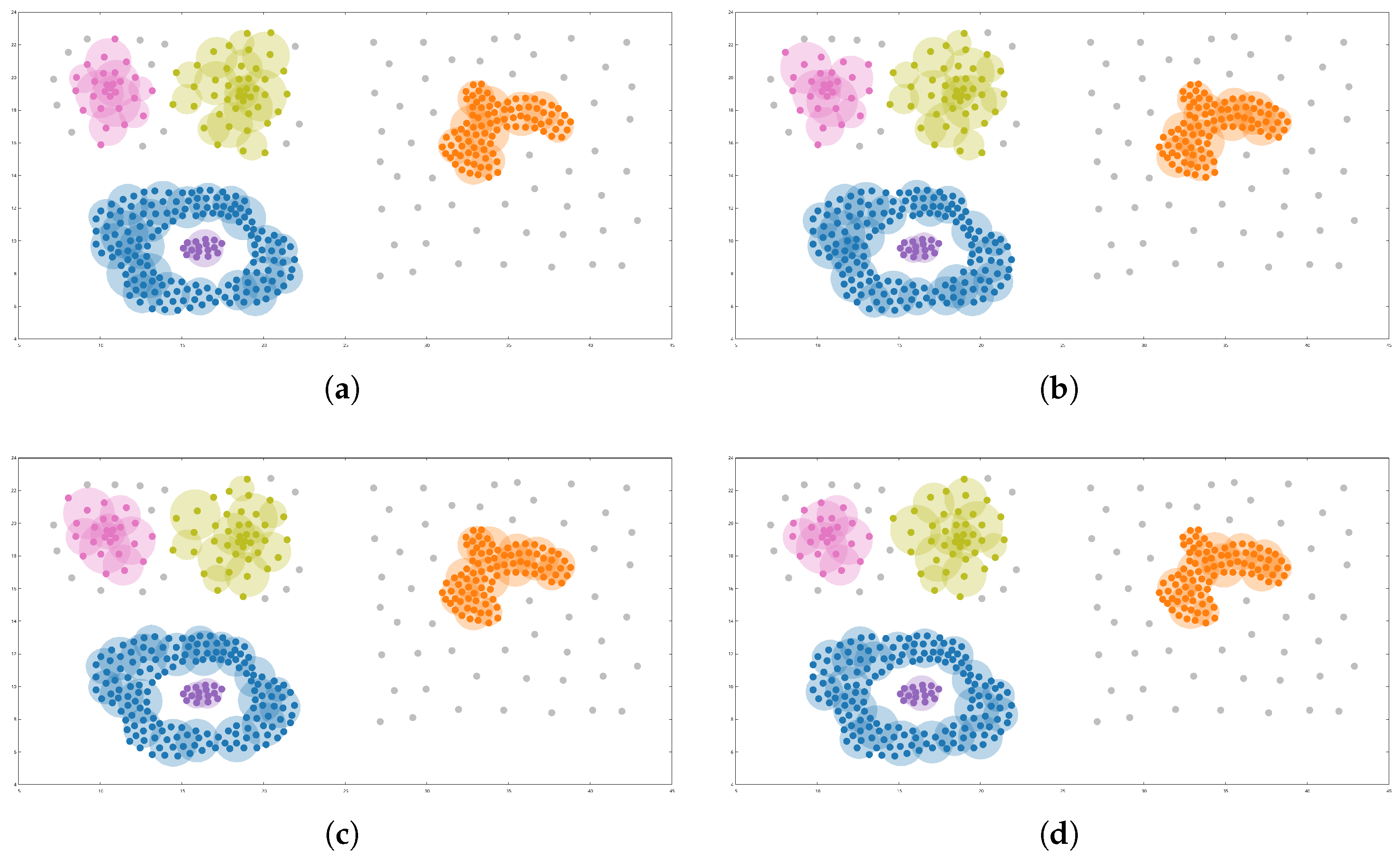
We executed the algorithm four times, using the same parameters while varying only the random seeds and orders in each run. For each execution, we recorded the clusters produced and the relevant object subsets used to build them. Figure 3 shows the results of these.

In this figure, objects labeled as noise are shown in gray, while the remaining objects are colored according to their assigned cluster. Larger circles represent the relevant object subsets identified by VDECAL, each colored to match its corresponding cluster. Figure 3 shows that all four runs converge to the same number of clusters with similar shapes. The objects in the concentric clusters (blue and purple) and the arbitrarily shaped cluster (orange) were always identified correctly, despite being derived from different relevant object subsets. The two remaining clusters (pink and green), which have ambiguous boundaries, were slightly affected by the algorithm’s random component. In Figure 3a, these clusters contained 27 and 43 objects, respectively; in Figure 3b, 28 and 42; in Figure 3c, 26 and 41; and in Figure 3d, 25 and 40 objects. The affected objects are located near cluster boundaries, where it is unclear whether an object belongs to one cluster or another or if it should be considered noise, which shows the VDECAL’s stability.

4.2. Quality

Three metrics were used to evaluate clustering quality, i.e., Adjusted Rand Index (ARI) [68], Adjusted Mutual Information (AMI) [69], and Normalized Mutual Information (NMI) [70], since these metrics are widely used in the literature for evaluating clustering algorithms. ARI adjusts for chance and measures the similarity between two clustering. AMI, also adjusted for chance, quantifies the shared information between the clusters and the ground truth, accounting for label distribution. NMI is based on Mutual Information (MI), which calculates how much knowing one clustering reduces the uncertainty about the other, and NMI normalizes this score. For all three metrics, a score of 1 implies a perfect matching. As the value decreases, the quality of the clustering also decreases.

All used metrics are external evaluation metrics and require labeled data to evaluate the clustering results. Therefore, we use a set of ten synthetic datasets (see

Table 1. Synthetic datasets used to evaluate clustering quality.

Dataset	Objects	Clusters	Dimensions
R15	600	15	2
Jain	373	2	2
complex8	2551	8	2
aggregation	788	7	2
Flame	240	2	2
2G_unbalance.txt	1050	2	2
Pathbased	300	3	2
Cluto-t4-8k	8000	7	2
Compound	399	6	2
Complex9	3031	9	2

) from the Tomas Barton’s repository [67], a benchmark widely used in the literature to evaluate density-based clustering algorithms. These datasets present diverse challenges, including arbitrary shapes, geometric shapes with noise, overlapping clusters separable by density, variations between clusters, smooth transitions between clusters, outliers, imbalanced clusters, differences in size and shapes, and the identification of weak connections, among others [71].

Since these datasets have been widely used for evaluating clustering algorithms, the parameter values that produce good clustering results for DBSCAN are well-known (${ϵ}_{dbs},minPt{s}_{dbs}$) [56]. Additionally, IKMEANS, KDBSCAN, KNN_BLOCK_DBSCAN, and our proposed algorithm (VDECAL) use the same parameters $ϵ$ and $minPts$. Thus, we employed these same values in our experiments and conducted further evaluations, changing these parameters values. For $ϵ$, we varied the values from ${ϵ}_{dbs}/2$ to $2{ϵ}_{dbs}$ with increments of 0.1, and for $minPts$, a range from 1 to $2minPt{s}_{dbs}$ with increments of 1. For those algorithms that require the number of nearest neighbors (K) as a parameter, such as RSDBSCAN and RNNDBSCAN, tests were conducted using values within the range of 2 to 30, with increments of 1, as recommended by the authors. For IKMEANS, which uses a sample size, the samples were established between 10% and 50% from the dataset size, in intervals of 5%. For those algorithms that require a number of partitions, such as KDBSCAN and RS-DBSCAN, the number of partitions was set between the range of 1 to 4 partitions. Finally, VDECAL requires the parameter $\delta$, the density variation threshold, to vary between 1 and 4 with increments of 0.1; moreover, the t parameter, defining the maximum partition size, takes values from 20% to 60% of the dataset size, with increments of 10%.

Table 2. Parameter values that produce the best-quality results.

Dataset	VDECAL	DBSCAN	IKM	KDBSCAN	RNNDBSCAN	RSDBSCAN	KNNBDBS
	($\mathit{t}$, $\mathsf{ϵ},\mathit{mPts},\mathsf{\delta }$)	($\mathsf{ϵ},\mathit{mPts}$)	($\mathsf{ϵ},\mathit{mPts}$)	($\mathit{P},\mathsf{ϵ},\mathit{mPts}$)	($\mathit{K}$)	(${\mathit{K}}_{\mathit{1}},{\mathit{K}}_{\mathit{2}}$)	($\mathsf{ϵ},\mathit{mPts}$)
R15	400, 0.5, 4, 3	0.35, 5	0.7, 1	2, 0.3, 1	12	2, 5	0.39, 5
Jain	200, 3.3, 1, 2.7	2.3, 4	2.6, 4	2, 2.26, 1	17	9, 4	2.34, 5
complex8	1300, 15.6, 3, 1.71	14.89, 4	11.3, 2	2, 14, 1	17	2, 10	14.9, 4
Aggregation	400, 1.8, 9, 1.9	1.6, 9	1.83, 2	2, 1.6, 9	14	2, 10	1.5, 8
Flame	120, 1.3, 4, 2.7	1.4, 9	1.45, 3	2, 1.45, 9	17	11, 3	1.4, 10
2G_unbalance	600, 0.14, 7, 2.7	0.1, 7	1.25, 1	2, 0.1, 4	14	3, 8	0.12, 9
pathbased	150, 1.7, 6, 2	1.6, 7	2.0, 2	2, 1.5, 6	11	3, 5	1.92, 8
cluto-t4-8k	4000, 9.7, 18, 2.4	9.5, 20	10.6, 2	2, 8.4, 15	16	3, 16	9, 15
compound	200, 1.5, 2, 3	1.3, 3	6.0, 4	2, 1.5, 2	10	5, 14	1.48, 3
complex9	1600, 15, 5, 2.7	12.1, 5	11.5, 2	2, 12.2, 1	25	2, 17	14.9, 5

shows the combinations of parameter values that produce the best-quality results for each algorithm.

Table 3. Performance on artificial datasets. Bold values indicate the best result(s) for each dataset.

Dataset	Metric	VDECAL	DBSCAN	IKM	KDBS	RNNDBS	RSDBS	KNNBDBS
R15	ARI	0.9927	0.9356	0.9264	0.8523	0.9891	0.9927	0.9500
	AMI	0.9938	0.9416	0.9591	0.9183	0.9907	0.9938	0.9544
	NMI	0.9942	0.9458	0.9626	0.9280	0.9913	0.9942	0.9577
Jain	ARI	1.0000	0.9349	0.3138	0.9420	1.0000	0.5313	0.9345
	AMI	1.0000	0.8476	0.5177	0.8795	1.0000	0.4141	0.8457
	NMI	1.0000	0.8485	0.5202	0.8800	1.0000	0.4154	0.8467
complex8	ARI	0.9723	0.9932	0.2360	0.9858	0.8735	0.5023	0.9490
	AMI	0.9737	0.9868	0.6085	0.9741	0.9239	0.6135	0.9472
	NMI	0.9739	0.9869	0.6168	0.9744	0.9245	0.6154	0.9478
aggregation	ARI	0.9956	0.9828	0.6318	0.9767	0.9956	0.9421	0.9781
	AMI	0.9923	0.9763	0.7588	0.9273	0.9923	0.9248	0.9705
	NMI	0.9924	0.9767	0.7638	0.9313	0.9924	0.9257	0.9710
Flame	ARI	0.9714	0.9387	0.3424	0.9396	0.9666	0.8229	0.9440
	AMI	0.9345	0.8722	0.5047	0.8873	0.9266	0.7293	0.8808
	NMI	0.9350	0.8731	0.5097	0.8880	0.9269	0.7302	0.8816
2G	ARI	0.9778	0.8244	0.0451	0.8565	0.9784	0.6592	0.8821
unbalance	AMI	0.9496	0.8094	0.1511	0.8369	0.9652	0.5411	0.8601
	NMI	0.9497	0.8102	0.1540	0.8377	0.9653	0.5421	0.8608
pathbased	ARI	0.9396	0.8032	0.5184	0.7738	0.5324	0.4671	0.8799
	AMI	0.9169	0.7799	0.5624	0.7381	0.5509	0.5319	0.8467
	NMI	0.9174	0.7813	0.5670	0.7454	0.5582	0.5362	0.8476
cluto-t4-8k	ARI	0.9522	0.9699	0.3878	0.9682	0.3866	0.6241	0.9709
	AMI	0.9376	0.9545	0.5011	0.9520	0.6595	0.6861	0.9575
	NMI	0.9377	0.9546	0.5017	0.9521	0.6618	0.6865	0.9576
compound	ARI	0.9385	0.9419	0.7957	0.9712	0.8817	0.6248	0.9634
	AMI	0.9305	0.9162	0.8372	0.9386	0.8994	0.6846	0.9315
	NMI	0.9320	0.9180	0.8403	0.9403	0.9020	0.6850	0.9330
complex9	ARI	1.0000	0.8806	0.4232	0.9470	0.9915	0.5480	0.9313
	AMI	1.0000	0.9491	0.6085	0.9525	0.9856	0.6852	0.9686
	NMI	1.0000	0.9494	0.6097	0.9527	0.9857	0.6864	0.9687

presents the best results of all the tests. These results show that our proposed algorithm, VDECAL, achieved the best result in 6 out of the 10 datasets evaluated, making it the top-performing algorithm. It was followed by RNNDBSCAN, which achieved the best results on three datasets, although in one, 2G unbalance was superior, and on the other two, Jain and aggregation RNNDBSCAN tied with VDECAL. It is important to highlight that both VDECAL and RNNDBSCAN are algorithms that consider density variations when building clusters. However, RNNDBSCAN is not designed for large datasets, which is reflected in the runtime experiments.

These experiments show that VDECAL achieved the best results on Jain, Aggregation, Flame, and Pathbased datasets. These datasets have clusters with arbitrary shapes and have density variations in continuous regions, which shows the proposed algorithm’s applicability to these kinds of datasets.

Detection of Density Variations

VDECAL’s ability to detect density variations allows it to create clusters that other algorithms cannot achieve. To illustrate this, we used a dataset named dense-disk-5000, also obtained from Tomas Barton’s repository [67]. This dataset has 5000 objects grouped in two clusters with different densities, the densest cluster is in the center of the dataset surrounded by a less dense cluster. The main characteristic of dense-disk-5000 is that there is no low-density area to separate the clusters; instead, there is a density variation between them (Figure 4a).

Upon analyzing the clusters built by the different algorithms with this dataset, we observed that DBSCAN marked the objects within the less dense cluster as noise (see the points in light gray), obtaining only the densest cluster (Figure 4b). However, this solution results in some information being discarded. KDBSCAN (Figure 4c) and KNN-BLOCK-DBSCAN (Figure 4d) have the same issue as DBSCAN. IKMEANS algorithm (Figure 4e) detected a high-density zone in the center of the dataset; however, the proximity among the objects of the less dense cluster leads to the incorrect detection of the cluster’s borders. The RNN-DBSCAN algorithm (Figure 4f) allows the detection of density variations, allowing it to separate the objects of the densest cluster; however, it cannot group the objects of the less dense cluster in a single cluster. Instead, it creates more clusters. The RS-DBSCAN algorithm (Figure 4g) built clusters similarly to RNN-DBSCAN, but the densest clusters’ borders were incorrectly identified. Finally, VDECAL (Figure 4h) detected density variations and can separate the objects into two clusters of different densities, resulting in a better separation of the two clusters.

4.3. Runtime

The datasets used in the quality evaluation pose challenges for cluster building; however, most of them contain a small number of objects, which limits the runtime analysis for large datasets. To assess this aspect, following Gholizadeh [54] and Hanafi [61], we used seven datasets from the UCI Machine Learning Repository [72], as they offer diversity in the number of dimensions and objects. In [54,61], values for $ϵ$ and $minPts$ are also suggested for each dataset, normalized within [0,1]. Consequently, we adopted these same values to set these parameters in the evaluated algorithms.

Table 4. Datasets and its parameters used in runtime evaluation.

Dataset	Objects	Dimensions	$\mathsf{ϵ}$	$\mathit{minPts}$
Abalone	4177	8	0.035	4
Dry_beam	13,611	16	0.16	4
Gas-drift	13,910	128	0.40	5
Magic	19,020	10	0.06	4
Letter	20,000	16	0.35	4
Nomao	34,465	118	1.98	5
Statlog (Shuttle)	58,000	9	0.02	5
Accelerometer	153,000	4	0.065	4
Skin Segmentation	245,057	3	0.01	4
Gas and position	416,153	9	0.003	20
3D Road Network	434,874	4	0.01	4
Poker-hand	1,000,000	10	0.25	10

shows the dataset name, the number of objects, the dimensions, and the values for $ϵ$ and $minPts$ used for IKMEANS, KDBSCAN, KNN_BLOCK_DBSCAN, and VDECAL. Additionally, IKMEANS uses a sample size parameter set to 10% of the dataset size, a value recommended by its authors. KDBSCAN and RS-DBSCAN use the number of partitions as a parameter, set to 5; higher values resulted in most of the dataset being marked as noise, preventing cluster formation. Our proposed algorithm, VDECAL, employs the $\delta$ parameter set to 2.5 for all the tests, a value experimentally determined to allow density variations. It also uses the t parameter, set to 20% of the dataset size, equivalent to creating five partitions. On the other hand, RNN-DBSCAN and RS-DBSCAN algorithms use a K parameter instead of these parameters, which was set to the same value as $minPts$, as recommended by the authors.

In this experiment, we analyze the runtime of six algorithms (VDECAL, RNNDBSCAN, RSDBSCAN, IKMEANS, KDBSCAN, KNN_BLOCK_DBSCAN) across the datasets listed in Table 4. Figure 5 shows the results on a graph with a logarithmic scale, where the runtime was recorded for each algorithm on each dataset; the datasets are ordered by increasing size and reported times to include effective CPU processing without input/output time. Note that if a dataset does not have a resulted runtime in the figure, it is because the algorithm exceeded 24 h, highlighting its limitations with large datasets.

KNN_BLOCK_DBSCAN processed 8 out of the 12 datasets, but exceeded the 24-h limit for the remaining four. Moreover, in all the datasets KNN_BLOCK_DBSCAN could process, it had the highest runtime out of the six clustering algorithms.

RNNDBSCAN and RSDBSCAN processed 11 out of the 12 datasets, but exceeded the 24-h limit for the largest dataset (Poker-hand). RNNDBSCAN’s runtime is among the highest. RSDBSCAN’s runtime exhibited a similar growth to RNNDBSCAN’s; however, RSDBSCAN outperformed RNNDBSCAN regarding runtime because it is an enhanced version for large datasets.

KDBSCAN processed 10 out of the 12 datasets. In medium-sized datasets such as Dry_beam, Letter, and Nomao, KDBSCAN outperformed VDECAL regarding runtime. However, as the size of the dataset increased, KDBSCAN’s runtime grew faster than VDECAL’s, making it unable to process the two largest datasets within the 24-h limit. In the Gas and Position dataset, although KDBSCAN’s runtime outperformed VDECAL’s and KDBSCAN’s runtime was 15 s while VDECAL’s runtime was up to 17 min, this variation on KDBSCAN’s runtime is because KDBSCAN marked all objects in the dataset as noise.

IKMEANS and VDECAL completed all 12 datasets within the 24-h limit. On the smaller datasets, VDECAL outperformed the IKMEANS runtime. On the largest datasets (Skin Segmentation, Gas and Position, 3D Road Network, and Poker-hand), IKMEANS shows better runtime compared to VDECAL. However, according to Section 4.2, IKMEANS is the algorithm with the worst clustering quality.

These results indicate that the proposed algorithm, VDECAL was faster than KNN_BLOCK_DBSCAN and RS-DBSCAN, which are the fastest, most accurate, and recent clustering algorithms for large datasets, with better or similar quality results.

4.4. Scalability

To assess VDECAL’s scalability, we conducted two experiments. The first experiment evaluates how the algorithm’s runtime scales with increasing dataset size by varying the number of objects. The second experiment evaluates the effect of data dimensionality on runtime, maintaining the number of objects fixed while varying the number of dimensions. The dataset used for these experiments is HIGGS, obtained from the UCI Machine Learning Repository [70]. This dataset has 11,000,000 objects, each with a dimensionality of 28. The parameters used for evaluation were set at epsilon = 1.0, minPts = 1100, and a partition size of 110,000. These parameters were chosen to generate two clusters within a reasonable runtime. While the clusters may not be optimal, they offer acceptable results given the time and computational limitations. We conducted each test ten times to account for the random component of VDECAL.

In the first experiment, we evaluated the scalability of VDECAL in terms of dataset size by increasing the number of objects. We used incremental portions of the HIGGS dataset, starting with 10% and progressively adding increments of 10% until reaching the full dataset size of 11,000,000 objects. Figure 6a depicts the results of how the runtime increases with the dataset size. The x-axis shows the portion of the dataset used, and the y-axis indicates the corresponding runtime (in minutes) required for VDECAL to process each portion. Each point in the figure has error bars, indicating the variability in runtime for the ten runs. Figure 6a shows that the VDECAL algorithm exhibits a proportional increase in runtime as the number of objects increases. This means that the algorithm scales well with increasing input size, as the runtime does not grow drastically. Thus, the VDECAL algorithm has good scalability, making it suitable for applications where the input size can vary significantly. The linear relationship between input size and runtime ensures predictable performance as the number of objects increases.

The second experiment evaluates the impact of data dimensionality on the runtime performance of VDECAL. For this experiment, we used only 10% of the original dataset. Initially, we used the 28 dimensions from the original dataset and progressively added 28 additional dimensions at each sample until we reached a total of 280 dimensions. To ensure that the distance between data objects does not change, all newly added dimensions were set to zero, which allows us to evaluate the impact of dimensionality on runtime without altering the data. Figure 6b depicts how runtime increases as the number of dimensions increases. The x-axis shows the number of dimensions, and the y-axis indicates the corresponding runtime (in minutes). Each point in the figure has error bars, indicating the variability in runtime for the ten runs. The results indicate that the runtime grows linearly as dimensionality increases. Figure 6b also shows that the runtime remains consistent across different dimensions, indicating that the VDECAL algorithm exhibits good scalability. In summary, both figures highlight the good scalability of VDECAL with increasing data size and dimensionality.

5. Conclusions and Future Works

This paper introduced VDECAL, a density-based clustering algorithm for efficiently handling large datasets. VDECAL operates through three stages. Initially, it partitions the dataset into segments of similar sizes to evenly distribute the computational workload. Subsequently, it identifies relevant object subsets characterized by attributes such as density, position, and overlap ratio, which are used for cluster building. Finally, using these relevant object subsets, VDECAL identifies low-density regions and density variations in the high-density regions to build the clusters. This way of building clusters enables VDECAL to reduce runtime without sacrificing clustering quality.

Our evaluation of VDECAL focuses on randomness, clustering quality, runtime performance, and scalability. Regarding randomness, our experiments show that VDECAL produces consistent results across different initial seeds and processing orders. Despite the random initialization, the algorithm consistently converges to similar clusters. Regarding clustering quality, from our experiments on a well-known repository widely used for assessing density-based clustering algorithms, we found that VDECAL shows quality improvement compared to state-of-the-art. The improvement in quality is obtained thanks to the density variation performed by our proposal, an unexplored approach in density-based clustering algorithms for large datasets.

Regarding runtime, the experiments show that our algorithm outperforms KNN BLOCK DBSCAN and RS-DBSCAN, the fastest, most accurate, and recent clustering algorithms for large datasets. Although IKMEANS was the fastest, its clustering quality is low compared to the other algorithms. The scalability experiments illustrate how VDECAL’s runtime changes when the number of objects and dimensions are increased. For dimensionality, VDECAL runtime is proportional to the number of dimensions. However, concerning the number of objects, VDECAL exhibits a slower growth rate, which is crucial when processing large datasets. This is achieved through the balanced distribution of workload proposed in the VDECAL partitioning stage.

The runtime efficiency of VDECAL relies on keeping a low number of relevant object subsets concerning the total dataset size, which is a limitation of our proposed algorithm. Another limitation is that in our proposed algorithm, the parameters require manual adjustment for each dataset. Future research could explore integrating statistical analysis techniques to detect density variations among relevant object subsets, potentially eliminating the need for specific thresholds as parameters. Additionally, considering the prevalent use of parallel processing techniques for accelerating computation and handling larger datasets, implementing VDECAL within frameworks such as MapReduce could offer promising improvements in scalability and performance.