AdaGram in Python: An AI Framework for Multi-Sense Embedding in Text and Scientific Formulas

Abstract

The Adaptive Skip-gram (AdaGram) algorithm extends traditional word embeddings by learning multiple vector representations per word, enabling the capture of contextual meanings and polysemy. Originally implemented in Julia, AdaGram has seen limited adoption due to ecosystem fragmentation and the comparative scarcity of Julia’s machine learning tooling compared to Python’s mature frameworks. In this work, we present a Python-based reimplementation of AdaGram that facilitates broader integration with modern machine learning tools. Our implementation expands the model’s applicability beyond natural language, enabling the analysis of scientific notation—particularly chemical and physical formulas encoded in LaTeX. We detail the algorithmic foundations, preprocessing pipeline, and hyperparameter configurations needed for interdisciplinary corpora. Evaluations on real-world texts and LaTeX-encoded formulas demonstrate AdaGram’s effectiveness in unsupervised word sense disambiguation. Comparative analyses highlight the importance of corpus design and parameter tuning. This implementation opens new applications in formula-aware literature search engines, ambiguity reduction in automated scientific summarization, and cross-disciplinary concept alignment.

1. Introduction

The exponential growth of digital text across scientific disciplines has intensified the need for models that can accurately capture semantic complexity and contextual variability. One of the most promising models in this regard is the Adaptive Skip-gram model (AdaGram), introduced by Bartunov et al. in 2016 [1].

AdaGram is a nonparametric Bayesian extension that avoids prespecifying model parameters by using probabilistic priors of the Skip-gram model, designed to learn multiple high-dimensional word representations that reflect distinct senses. These representations capture rich semantic relationships between words while accounting for word ambiguities by learning the required number of representations with an appropriate semantic resolution [1]. Unlike traditional word embedding models that learn a single representation per word, AdaGram distinguishes between multiple meanings, making it particularly well-suited for tasks involving polysemy and homonymy.

One of AdaGram’s key advantages is its ability to disambiguate word senses in an unsupervised manner. This is particularly important in domains such as natural language processing (NLP) and information retrieval, where context-specific meaning plays a critical role [2,3,4]. Using a Bayesian formulation and flexible context modeling, AdaGram can outperform classical Skip-gram models in capturing nuanced semantic relationships across heterogeneous corpora [1]. Crucially, the number of senses per word is not predefined. Instead, it is inferred directly from the data through the Bayesian framework, enabling dynamic representation learning.

Recent studies have demonstrated AdaGram’s efficacy in word sense induction and disambiguation tasks, achieving state-of-the-art results on standard benchmarks [5,6,7,8]. Beyond NLP, AdaGram has shown promise in other domains. For example, Tshitoyan et al. (2019) [9] applied AdaGram-based embeddings to the materials science literature and uncovered latent patterns that enabled the prediction of material properties years in advance. This led to the hypothesis that “latent knowledge regarding future discoveries is largely embedded in past publications,” highlighting AdaGram’s capacity to uncover hidden semantic structures in specialized domains.

These successes motivated our re-implementation of AdaGram in Python, a language more widely adopted in the machine learning community than Julia. Python’s robust ecosystem enables seamless integration with major libraries, including TensorFlow 2.18.0, PyTorch 2.7.1+cu126, and Scikit-learn 1.7.0.

In addition, our version extends AdaGram to process scientific notation—particularly LaTeX-encoded formulas—which pose unique challenges for traditional text models due to their structural and symbolic complexity.

While AdaGram has demonstrated utility in materials science, we hypothesize that its broader application across scientific fields such as bioinformatics, chemistry, physics, and systems biology can support semantic extraction and sense disambiguation in texts combining natural and symbolic language. Recent trends in hybrid knowledge representation integrate neural embeddings with symbolic and structural modeling [10,11,12,13,14,15,16]. For example, terms such as ‘delta’ or ‘H’ can have different meanings in physics, thermodynamics, and chemistry. AdaGram’s ability to learn multiple senses makes it ideally suited for such ambiguity-rich contexts.

In this work, we contribute a Python-based implementation of AdaGram focused on interdisciplinary applications, especially scientific formulas. Our primary goals are to (1) evaluate the behavior of the model in diverse corpora; (2) demonstrate its effectiveness in extracting semantic distinctions from scientific formulas; (3) investigate how hyperparameter tuning affects disambiguation performance; and (4) compare with existing BERT [17] models to highlight the discovery of senses for the given text. Building on AdaGram’s Bayesian foundation, our goal is to provide a model that is not only algorithmically robust but also versatile in practice.

Ultimately, our objective is to bridge the gap between linguistic models and scientific reasoning by enabling semantic analysis of both natural and symbolic language. This includes potential applications in semantically dense domains such as chemical notation, biomedical equations, and molecular code modeling [18,19,20,21], where accurate disambiguation is essential for inference and knowledge discovery. In contrast to transformer-based embeddings such as BERT, which require large pretraining corpora and exhibit implicit sense representation, AdaGram explicitly models multiple senses in a probabilistic framework, offering a lightweight yet interpretable alternative for domain-specific disambiguation [22].

To the best of our knowledge, this is the first detailed Python-based implementation of AdaGram specifically adapted for structured scientific notation, such as LaTeX-encoded chemical and physical formulas.

2. The AdaGram Algorithm and Preprocessing Pipeline

Adaptive Skip-gram (AdaGram) is a nonparametric Bayesian extension of the widely used Skip-gram model, originally implemented in the word2vec software. word2vec software by Google—accessed via Google Code Archive (https://code.google.com/archive/p/word2vec/, accessed on 7 July 2025).

Unlike the original Skip-gram, which learns a single vector per word, AdaGram learns multiple vector representations to capture distinct meanings in different contexts. Importantly, the number of senses is not specified a priori but is inferred from the data. The original AdaGram implementation was developed in the Julia programming language [1].

2.1. Basics of AdaGram

Natural language is inherently ambiguous, as many words exhibit polysemy (multiple related meanings) or homonymy (distinct, unrelated meanings with the same form). For instance, the word “bank”can refer to a financial institution or the side of a river. The classical Skip-gram model assigns a single vector representation to each word, which is insufficient to model these ambiguities. AdaGram addresses this limitation by learning multiple embeddings for each word, with each vector representing a distinct sense derived from contextual usage [1].

AdaGram builds on the Skip-gram model but introduces several key innovations:

2.1.1. Multiple Embeddings

Each word w is represented not by a single vector, but by a set of vectors $\left\{v_{w,z}\right\}$, where z indexes the different meanings (or senses) of the word. This allows the model to capture semantic diversity by assigning distinct embeddings to each usage context. For example, a word with two senses—such as “rock” which means “stone” or “music genre”—would be associated with two separate vectors, each reflecting its respective meaning.

2.1.2. Bayesian Approach

AdaGram treats the sense of a word as a latent variable z. For a given word w, the sense z is drawn from a probability distribution $P\left(z\right|w)$, which is modeled using the softmax function:

$$P\left(z\right|w)={\displaystyle \frac{exp\left(\varphi \right(w,z\left)\right)}{{\sum }_{z^{\prime }}exp\left(\varphi (w,z^{\prime })\right)}},$$

(1)

where $\varphi (w,z)$ measures the relevance of sense z for word w.

2.1.3. Context Modeling

Given a word w and its sense z, the probability of observing a context c is:

$$P\left(c\right|w,z)=\prod _{c_i\in \mathrm{context}}P\left(c_i\right|w,z),$$

(2)

where $P\left(c_i\right|w,z)$ is modeled using the dot product of the embeddings:

$$P\left(c_i\right|w,z)\propto exp\left(v_{c_i}^{\top }{v}_{w,z}\right).$$

(3)

AdaGram employs the Expectation-Maximization (EM) algorithm:

• E-step: Compute the posterior distribution $P\left(z\right|w,c)$ over senses given the word and its context.
• M-step: Update the embeddings $v_{w,z}$ and relevance scores $\varphi (w,z)$ to maximize the likelihood.

2.1.4. Advantages

• Handling Polysemy: AdaGram explicitly models multiple meanings, providing a nuanced representation of words.
• Context Sensitivity: The model dynamically selects the appropriate meaning of a word based on its context.
• Bayesian Framework: The probabilistic nature allows for robust handling of sparse data.

2.1.5. Applications

• Word Sense Disambiguation: AdaGram is well-suited for disambiguating word senses based on context.
• Semantic Similarity: By modeling multiple embeddings, the algorithm captures fine-grained semantic relationships.
• Language Modeling: AdaGram enhances language models by incorporating context-sensitive predictions.

2.1.6. Limitations

• Computational Complexity: The introduction of multiple embeddings increases both memory and computational cost.
• Hyperparameter Tuning: Determining the number of senses per word requires careful adjustment.
• Interpretability: The resulting embeddings require post hoc analysis to interpret the senses.

The AdaGram algorithm represents a significant advancement in word representation models by addressing the limitations of single-vector embeddings. Its ability to model polysemy and adapt to context makes it a powerful tool for natural language processing tasks. Future work could explore integrating AdaGram with other deep learning architectures to further enhance its capabilities.

2.2. Python Implementation

2.2.1. Data Cleaning

The training text must be words separated by spaces, so no punctuation marks can be left in the text file. This step can be skipped for texts that do not have clutter. However, for natural texts extracted from Wikipedia, Scopus, or other articles found online, data cleaning is an essential step for the success of this tool.

Since the text file is a list of strings, removing clutter can be done using Python’s (version 3.10.12) re module.

• Removing starting and ending whitespaces
• Removing clutter
  When extracting online text, there might be HTML tags, URL links, or other artifacts merged with the actual article. We could remove the punctuation, but that would not eliminate the tags themselves. For example: <title> would be turned into title, and it is not a relevant word for the text we would like to train on.
  This is when to use the Python re module (Regular Expressions) to detect the pattern of the strings we want to remove.
  •         # Pattern to remove HTML/CSS artifacts (e.g., <div>, </span>)
            re.search(r"^([\d]|[^\w\s])+[a-zA-Z]+([\d]|[^\w\s]*)+", word)
  This searches for a pattern that matches one or more punctuation marks, then one or more letters, then zero or more punctuation marks. (Ex: “<ref” or “</ref>”)
  Filter URLs and mixed alphanumeric strings (e.g., H2O remains intact)
  re.search(r"^[a-zA-Z]+([\d]|[^\w\s])+[a-zA-Z]*", word)
  This searches for a pattern that matches one or more letters, then one or more punctuation marks, then zero or more letters. (Ex: https://www.youtube.com (accessed on 15 June 2025))
          re.search(r"[0-9]",word)
  This searches for a pattern that has a number. (Ex: 20th, 2nd, 2, etc.)
  If the word you are checking fits any of the search functions above, then you can ignore it and move on to the next word.
  Note: This rule applies only to natural language corpora. For scientific texts (e.g., chemical formulas), a separate tokenization pipeline is employed to retain digits and subscripts necessary for semantic interpretation.
• Lemmatization and stop word removal
  One word may have different forms. The word “program” can be “programmed”, “programs”, or “programming”, which are all different forms but have the same meaning. The method used to reduce all forms of a word into one is lemmatization, and we need to apply it to avoid repetition during training.
  Stop words are frequently used words that serve no meaning to a text when you are training. Examples of these stop words are pronouns (“I”, “are”, “you”, etc.), “a”, “the”, and others.
  The following code sample, using nltk (Python’s natural language toolkit) serves the purpose of lemmatization and removing the stop words:
          wntag = pos_tag(word)[0].lower()
          newword = lemmatizer.lemmatize(word,wntag) if wntag in
          [’j’, ’r’, ’n’, ’v’] else ""
          if not (newword in ENGLISH_STOP_WORDS):
             newlist.append(newword)
  The lines above state that after taking the first letter of a given word’s tag (“v” for a verb, “n” for a noun, etc.), we will lemmatize the word based on that tag. So, the word “better” would turn to “good”, the word “studies” would turn to “study”, and so on.

2.2.2. Dictionary Creation

Once the text cleaning is done, we prepare a dictionary file as an additional parameter to the training, where the file details each word in the cleaned text along with its frequency:

        word1 45

        word2 413

        ...

        wordN 12

A dictionary file can be created by using the Counter subclass in Python to count the frequencies of the words.

2.2.3. Training

Similar to the Julia implementation, the way to train a model is to run the train.py program. To run it properly, these parameters must be taken into consideration [1]:

• window: a half-context size (Default value: 4).
• workers: specifies how many parallel processes will be used for training (Default value: 1).
• min-freq: sets the minimum word frequency below which a word will be ignored (Default value: 20).
• remove-top-k: allows ignoring the K most frequent words.
• dim: is the dimensionality of the learned representations (Default value: 0).
• prototypes: defines the maximum number of prototypes learned (Default value: 5).
• alpha: is a parameter of the underlying Dirichlet process (Default value: 0.1).
• d: is used in combination with alpha in the Pitman–Yor process, and d=0 turns it into a Dirichlet process (Default value: 0).
• subsample: is a threshold for subsampling frequent words (Default value: inf).
• context-cut: allows a randomly decreasing window during training, increasing training speed with negligible effects on model performance.
• init-count: initializes the variational stick-breaking distribution. All prototypes start with zero occurrences except for the first one, which is assigned the init-count. A value of zero means that the first prototype receives all occurrences (Default value: 1).
• stopwords: is the path to a newline-separated file containing words to be ignored during training.
• sense-threshold: allows sparse gradients, speeding up training. If the posterior probability of a prototype is below this threshold, it will not contribute to parameter gradients (Default value: 1 × 10⁻¹⁰).
• save-threshold: is the minimal probability of a meaning to save after training (Default value: 1 × 10⁻³).
• regex: filters words from the dictionary using the specified regular expression.
• train: path to the training text.
• dict: path to the dictionary file.
• output: path for saving the trained model.

We have added one more parameter to the original code: words-to-track. When using this parameter, you would provide the terminal a list of words that you would like to track for plotting the beta distributions of their prototypes after training.

Most of the parameters have default values, so you can run the training just by typing the following in the terminal:

    run training.py --dict dict_example.txt --train cleaned_example_text.txt

    --output example_model.txt

Exploration of some parameters and the differences found when changing their values can be seen in Section 3.

2.2.4. Model Usage

To use the model and examine it, you must first load the model and the dictionary:

    vm, dictionary = load_model("/.../AdaGram_Python/example_model.txt")

The vector model would then be supplied with the word vectors, the number of words, and their meaning(s).

A word might have multiple meanings depending on the context it is in. To check how many meanings were captured, we use the initialise-expected-pi function. As an example, we will use the word “rock”:

    In[1]: initialize_expected_pi(vm,dictionary.word2id["rock"])

    Out[1]: array([3.79346417e-01, 6.20543181e-01, 1.00377930e-04,

            9.11222056e-06, 9.11416223e-07])

The output is an array of probabilities for the five meanings the word “rock” could have. Since there are only two probabilities that are significantly larger than zero, it is safe to assume that two meanings for “rock” were captured. This is validated because “rock” can mean a music genre or a stone.

Note that “rock” has a third meaning, which is to move back and forth, but if the text you have trained does not contain any contexts related to that meaning, then it will not be reflected in the vector model.

Another function to use to test the validity of the model is disambiguate-call. When you pass a context as a parameter, the function’s output should be an array of probabilities that match the probabilities in the initialise-expected-pi function.

For example, when passing the parameter “roll music band album”, it should show a higher probability to one of the first two contexts and a lower one for the other.

    In[2]: disambiguate_call(vm,dictionary,"rock",

            "roll music band album".split())

    Out[2]: array([6.65383844e-01, 2.74887688e-04, 1.11449180e-01,

            1.11446044e-01, 1.11446044e-01])

This shows that the music genre meaning for “rock” was captured in the first context.

    In[3]: disambiguate_call(vm,dictionary,"rock",

            "sediment igneous mineral earth".split())

    Out[3]: array([1.99545790e-05, 6.54750351e-01, 1.15048947e-01,

            1.15090374e-01, 1.15090374e-01])

This shows that the stone meaning of “rock” was captured in the second context.

These examples provide early evidence that AdaGram can distinguish contextually distinct senses under controlled settings. However, robust validation across larger annotated datasets is required for definitive conclusions.

2.2.5. Adaptation to Scientific Formulas

Traditional word-embedding techniques often struggle with scientific formulas due to their specialized notation and structure. We adapted the AdaGram algorithm to handle chemical and physical formulas by implementing custom tokenization and preprocessing strategies.

Specialized Tokenization

While standard text tokenization treats words as atomic units, scientific formulas require decomposition at multiple levels. Our approach recognizes both complete formulas (e.g., H₂O) and their constituent components (H, 2, O) as meaningful tokens (Algorithm 1):

Algorithm 1 Formula Tokenization Strategy

1: Extract formula content within \ce{} tags 2: Process reaction arrows (→, ↔, ⇌) 3: Handle arithmetic operators (+, −) 4: Tokenize at two hierarchical levels:      Complete chemical entities (e.g., H2O, Fe3+)      Component elements and subscripts (H, 2, O) 5: Extract specialized notation:      Thermodynamic symbols ($\Delta H$, $\Delta G$, $K_a$)      Quantum mechanical notation ($\Psi$, subscripted variables)

Regex-Based Extraction

We implemented regular expression patterns to identify and extract formula components from LaTeX markup:

• Chemical formulas with subscripts and superscripts;
• Charges and oxidation states;
• Complex groups in parentheses and brackets;
• Reaction arrows and equilibrium symbols;
• Thermodynamic and quantum mechanical notation.

This approach allows our embedding model to learn meaningful representations at multiple granularities, from individual elements to complete reaction mechanisms. We further discuss this in Section 3.9.

Corpus Frequency Analysis

Statistical analysis of our corpus revealed unique characteristics of formula-based text compared to natural language:

• Higher frequency of specialized symbols and operators;
• Multi-level hierarchical structures (e.g., nested parentheses in complex formulas);
• Context-dependent meaning of subscripts and superscripts;
• Domain-specific notation systems.

Our tokenization algorithm directly addresses these challenges through specific design choices. The dual-level tokenization (Algorithm 1, steps 4–5) captures both complete formulas and their components, allowing the model to learn representations at multiple granularities, addressing the hierarchical nature of chemical notation. The explicit handling of specialized symbols (steps 2–3, 5) ensures that operators like reaction arrows and thermodynamic symbols are preserved as meaningful tokens rather than fragmented tokens. Context-dependent subscripts and superscripts are maintained within their parent entities during the complete formula tokenization phase, while also being available as separate tokens for compositional understanding.

This approach enables the embedding model to distinguish between H₂O as a complete molecular entity and its constituent elements H, 2, and O, while preserving domain-specific relationships between symbols like $\Delta H$ and thermodynamic contexts. The adaptive sense disambiguation capabilities of AdaGram are thus enhanced by this structured representation of scientific notation.

3. Results, Evaluation, and Test Cases

3.1. Real-World Texts

Testing the tool using natural text found in the real world would require a corpus with two or more contexts for a given word. To do this, we use polysemous words.

For the purpose of this evaluation, the word “rock” will be tested. The text file we use for training is a combination of Wikipedia articles for Rock (Music) (https://en.wikipedia.org/wiki/Rock_music) and Rock (Geology) (https://en.wikipedia.org/wiki/Rock_(geology)) (both accessed on 15 June 2025).

When training with the default parameters, the AdaGram tool provides us with these probabilities:

    In[11]: initialize_expected_pi(vm,dictionary.word2id["rock"])

    Out[65]:

    array([9.99891131e-01, 9.89719735e-05, 8.99685883e-06, 8.17896255e-07,

            8.17896255e-08])

Despite what was provided, only one meaning for the word “rock” was captured by the vector model. We observe that the size of the training corpus significantly impacts the model’s ability to learn distinct senses, especially when dealing with subtle semantic differences.

There are some parameters we could modify to mend this: alpha leads to more meanings with larger values, and increasing epochs is beneficial for smaller text [1], see Figure 1.

To better visualize the relative importance of each distribution component, we also present the same data on a linear scale in Figure 2. This representation highlights the dominance of the first few components and reveals how different parameter combinations distribute probability mass across the components.

What can be gleaned from these figures is the inefficiency in changing alpha alone. The training text’s size becomes 34,000 words when epochs = 2, but it does not display two contexts. However, when epochs $\ge 5$, the model learns multiple meanings. The linear scale representation in Figure 2 makes it particularly clear how configurations with higher epoch values (especially epochs = 10 and epochs = 15) distribute substantial probability mass to components $\pi$2 and $\pi$3, indicating the model’s increasing tendency to identify multiple word senses.

Since epochs = 10 and epochs = 15 make the model learn more than the two intended contexts, it would seem that increasing the epochs to any large number would not benefit small text. It could interpret patterns that should not be present. As such, the best test cases to run disambiguate-call on are when epochs = 5 and alpha = 0.2, epochs = 2.

To further analyze the computational characteristics of different parameter configurations, we present comprehensive performance visualizations for both the Apple and Rock datasets. These analyses provide crucial insights into the trade-offs between training time and memory usage across various combinations of alpha and epochs parameters, as referenced in

Table 1. List of Parameter Tests for the disambiguate-call Function.

#	Parameter Values	Music Context for “Rock”	Stone Context for “Rock”
1	epochs = 5	[0.00154198, 0.47751509, 0.17364764, 0.17364764, 0.17364764]	[0.58478621, 0.03064677, 0.12818901, 0.12818901, 0.12818901]
2	alpha = 0.2, epochs = 2	[0.00332149, 0.24225809, 0.25147347, 0.25147347, 0.25147347]	[0.79822595, 0.01363814, 0.06271197, 0.06271197, 0.06271197]

.

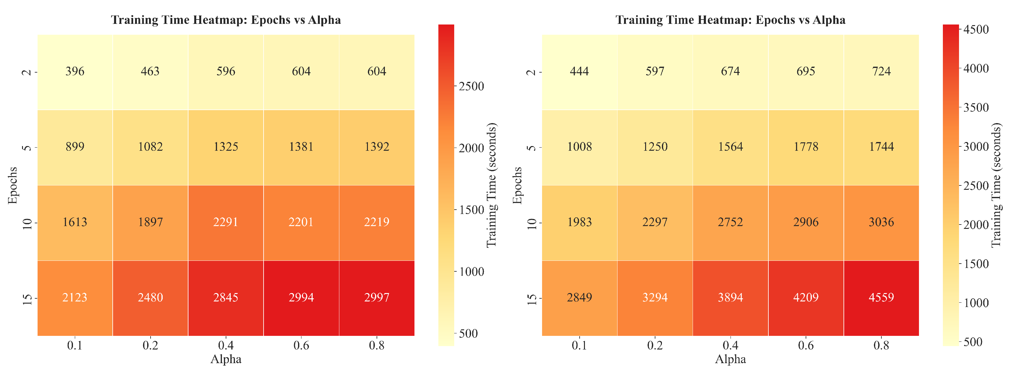
3.2. Training Time Heatmap Analysis

We begin with heatmap visualizations that provide an overview of the training-time landscape across the entire parameter space for both datasets.

The heatmaps in Figure 3 reveal several important patterns in computational performance. Training time generally increases with higher epochs values, as expected due to the iterative nature of the algorithm. The relationship with alpha shows more complex behavior, with certain ranges providing optimal computational efficiency. Most notably, the Rock dataset consistently demonstrates substantially lower computational requirements compared to the Apple dataset, with training times ranging from approximately 400–4500 s versus 300–2500 s, respectively. This difference suggests that intrinsic dataset characteristics such as dimensionality, complexity, and convergence properties significantly influence algorithmic computational demands.

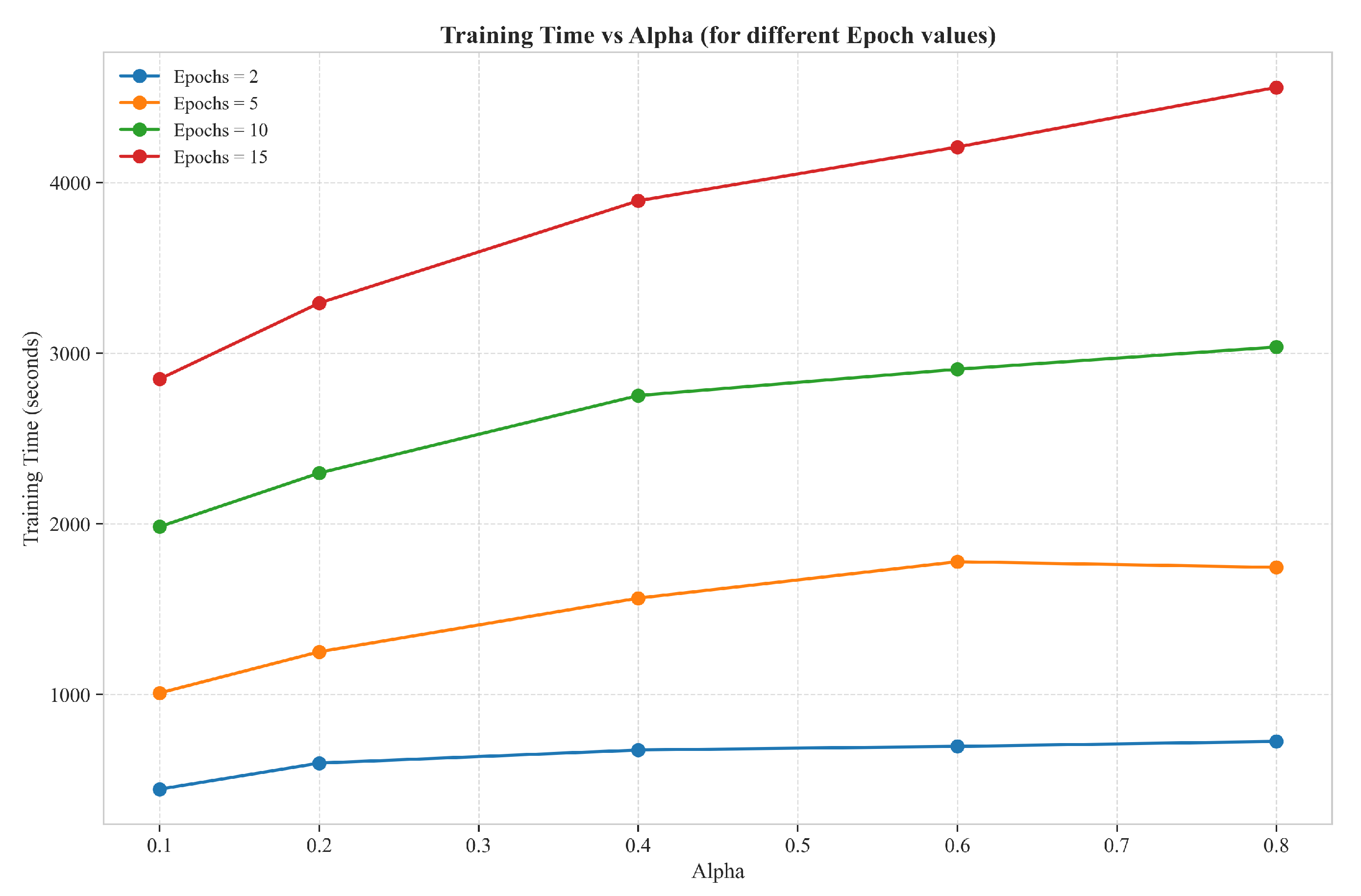
3.3. Cross-Sectional Training Time Analysis

To complement the surface visualizations, we examine how training time varies along specific parameter trajectories, providing detailed insights into scaling behavior.

The detailed training time analysis in Figure 4 reveals several critical insights for the Rock dataset. The relationship between alpha and training time is approximately linear for all epoch configurations, but the slope varies significantly with the number of epochs. For lower epoch values (2 and 5), training time remains relatively stable across the alpha range, making these configurations attractive for applications with strict time constraints.

The 10-epoch configuration shows moderate scaling, while the 15-epoch setting demonstrates the steepest increase in computational cost as alpha increases. This pattern suggests that higher alpha values require more computational effort to achieve convergence when combined with extended training periods, likely due to increased model complexity and more refined prototype adjustments during each iteration.

3.4. Computational Efficiency Implications

Memory usage patterns demonstrate that certain parameter combinations create significantly higher resource demands. This is particularly evident in configurations with both high epochs and specific alpha ranges, where the model maintains multiple prototype distributions simultaneously. The Rock dataset’s generally lower memory requirements compared to typical text processing tasks can be attributed to differences in vocabulary size and document complexity characteristics.

These performance characteristics directly inform our parameter selection strategy. For the Rock dataset, where we observed that epochs = 5 and alpha = 0.2 provide optimal semantic disambiguation, the performance analyses confirm that these configurations also represent computationally efficient options. Specifically, the epochs = 5 configuration achieves reasonable training times (approximately 1500 s) while avoiding the steep computational costs associated with higher epoch values.

The alignment between semantic quality and computational efficiency makes these parameter combinations particularly attractive for practical applications. The analysis reveals that moderate values of both alpha and epochs often provide the best trade-offs, avoiding the computational overhead of extreme parameter values while maintaining high-quality topic modeling results.

Furthermore, the contour analysis identifies parameter regions where small changes can lead to significant computational savings without substantially impacting model quality. This insight is particularly valuable for large-scale applications where computational resources are constrained, enabling practitioners to make informed decisions about parameter selection based on both performance requirements and available computational budget.

In Table 1, altering the alpha and epochs parameters together reveals that the stone context is represented in the first prototype, but it does not show as well for the music context. It can be inferred in this case that having multiple epochs is an essential parameter for smaller texts. Further testing is needed to understand the full spectrum of the AdaGram parameters.

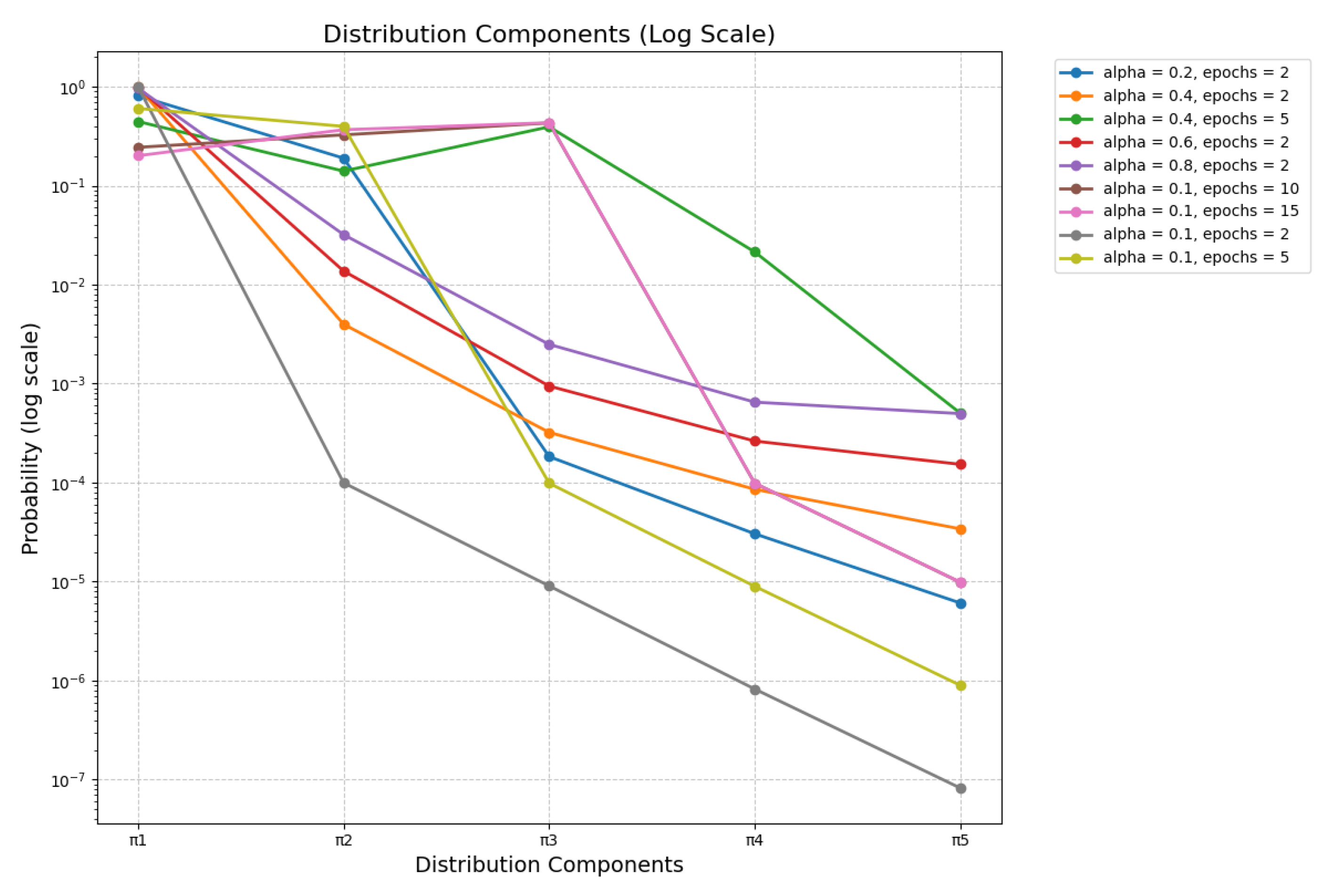
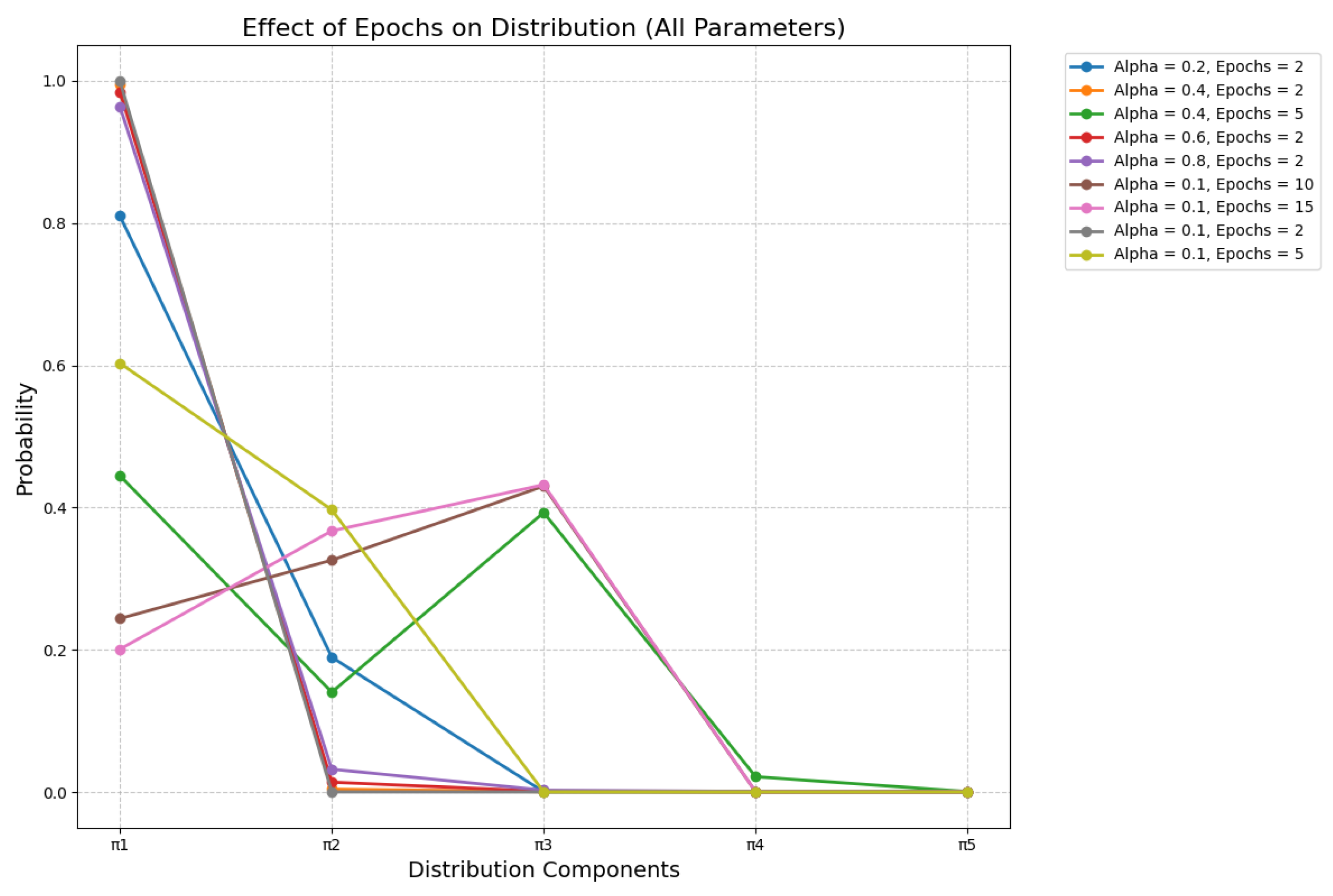
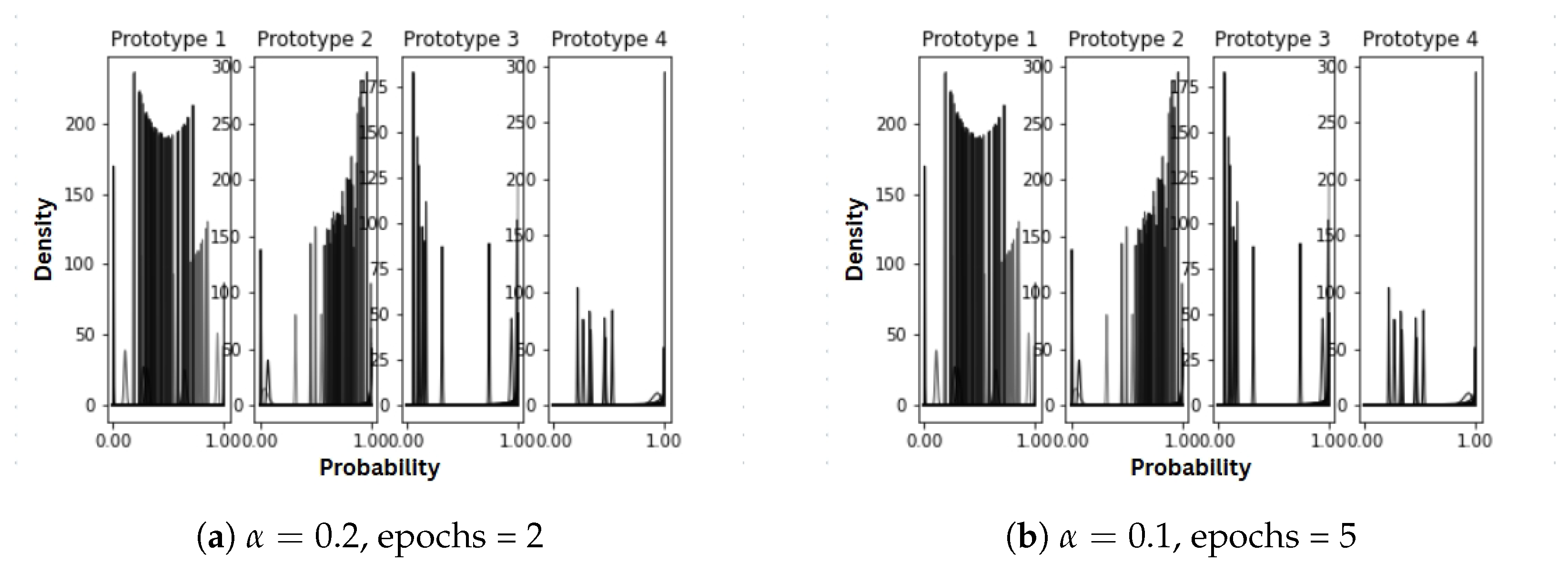
3.5. Beta Distributions in Sense Modeling

AdaGram uses a nonparametric Bayesian approach, specifically a stick-breaking process, to model the distribution over senses for each word. This results in a prior over senses that follows a Beta distribution when truncated, allowing the model to represent an open-ended number of prototypes. The concentration parameter alpha and the discount parameter d control the sparsity and shape of this distribution.

Empirical results, as shown in the outputs of the initialize_expected_pi function, reveal the probabilities assigned to each prototype. These distributions often show one or two dominant components and several vanishing ones. This behavior is theoretically consistent with the Beta prior underlying the Dirichlet process [23], which favors sparse allocations of probability mass unless corpus evidence strongly supports otherwise.

Visualizing these distributions during training, especially for controlled data, can provide valuable insight into how well the model is capturing sense structure. Prior work in probabilistic topic modeling has used similar visualizations to interpret latent distributions over document topics [24].

Figure 5 illustrates how Beta distributions for the polysemous word “rock” evolve under different hyperparameter settings and training durations. The comparison reveals the influence of the concentration parameter $\alpha$ and training duration on sense disambiguation. With a higher $\alpha$ value and fewer epochs (panel a), the model maintains relatively more uncertainty across potential senses. In contrast, with a lower $\alpha$ value and more training epochs (panel b), the model exhibits increased certainty in sense assignments, demonstrating the expected behavior where the concentration parameter controls the dispersion of probability mass across prototypes. In both cases, Prototype 1 emerges as the dominant sense, while the distributions for secondary senses (Prototypes 2 and 3) show interesting variations that reflect the model’s adaptation to corpus evidence under different prior constraints.

3.6. Performance Analyses

To comprehensively evaluate the computational characteristics of different parameter configurations, we present detailed performance visualizations for both the Apple and Rock datasets. These analyses provide crucial insights into the trade-offs between training time, memory usage, and overall computational efficiency across various combinations of alpha and epochs parameters.

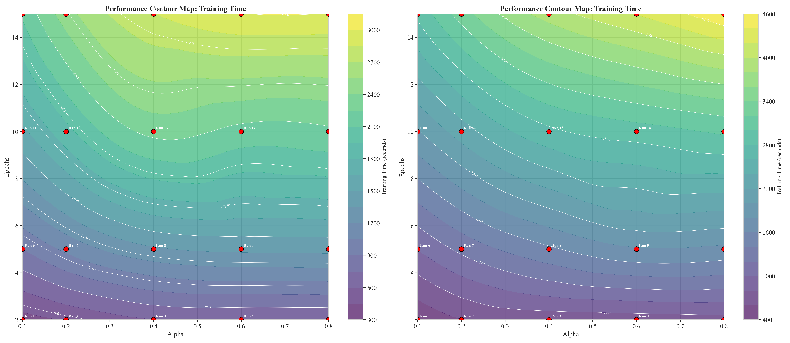
3.6.1. Training Time Contour Map Analysis

The training time contour maps reveal the computational landscape across parameter space, highlighting regions of optimal efficiency and identifying parameter combinations that minimize computational cost.

The contour maps in Figure 6 reveal several critical patterns in computational efficiency. Training time exhibits a clear gradient across both datasets, with lower epochs and moderate alpha values generally providing the most efficient computation times. The contour lines demonstrate that the relationship between parameters and training time is non-linear, with certain parameter combinations creating computational bottlenecks.

Notably, the Apple dataset shows more pronounced computational variations across the parameter space compared to the Rock dataset, suggesting that the Apple dataset’s characteristics make it more sensitive to parameter selection from a computational efficiency perspective. The contour density patterns indicate specific regions where small parameter changes can lead to significant computational cost differences, which is crucial information for parameter optimization strategies.

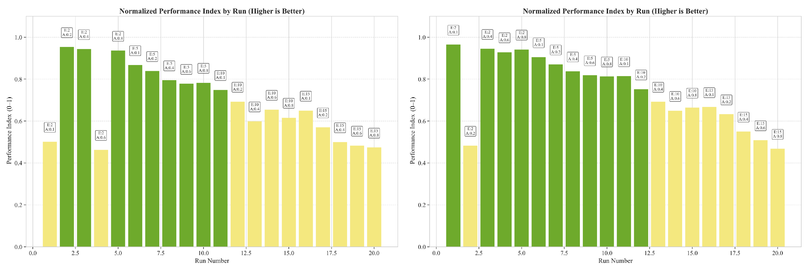
3.6.2. Normalized Performance Index

To assist in parameter selection, we propose a normalized performance index combining training time and memory usage. While this is not a validated benchmark metric, it serves as a practical tool to compare resource efficiency across configurations.

The performance index visualization in Figure 7 provides actionable insights for parameter selection. The index combines normalized training time and memory usage (with equal weighting) into a single metric where higher values indicate better overall performance. This approach identifies configurations that achieve an optimal balance between computational efficiency and resource utilization.

For the Apple dataset, runs with lower epochs (E:2–5) consistently achieve higher performance indices, particularly when paired with moderate alpha values (A:0.1–0.4). The Rock dataset shows similar patterns but with slightly different optimal ranges, confirming that dataset characteristics influence the ideal parameter space while maintaining consistent general trends.

3.6.3. Performance Optimization Guidelines

Based on the comprehensive performance analysis, we establish the following parameter selection guidelines:

High Performance Configurations:Parameter combinations achieving performance indices above 0.8 consistently demonstrate epochs ≤5 and alpha values in the range 0.1–0.4. These configurations provide excellent computational efficiency while maintaining model quality.

Moderate Performance Range: Configurations with performance indices between 0.5–0.8 typically involve moderate epochs (5–10) or higher alpha values (0.4–0.6). These represent reasonable trade-offs when specific model requirements necessitate these parameter ranges.

Resource-Intensive Configurations: Parameter combinations with performance indices below 0.5 generally involve high epochs (≥10) combined with elevated alpha values (≥0.6). While these may provide enhanced model sophistication, they come at a significant computational cost.

The convergence of semantic quality findings with computational efficiency analysis strongly supports our earlier conclusion that epochs = 5 with alpha = 0.2 represents an optimal configuration for practical word sense disambiguation applications. The (epochs = 5, alpha = 0.2) setting effectively disambiguates homonyms like rock while maintaining computational efficiency, making it a pragmatic choice for both research and production.

While the current study uses moderate-sized corpora, future work will explore training on larger, more heterogeneous datasets to evaluate model scalability. Preliminary experiments suggest that training time increases sublinearly with corpus size for fixed parameters, though memory usage scales with the number of prototypes retained. Dataset-specific factors such as vocabulary diversity and context density further influence resource requirements.

3.7. Comparative Analysis of AdaGram with Original AdaGram and BERT Models

To evaluate the effectiveness of our Python AdaGram implementation, we conducted a comprehensive comparative analysis using four distinct methodologies: three contextual BERT-based embeddings bert-base-uncased, SciBERT, SenseBERT) and our Python AdaGram implementation. This evaluation primarily focuses on qualitative assessment, with the comparison against contextual embeddings serving to illuminate AdaGram’s distinctive capabilities in identifying discrete semantic clusters with minimal supervision.

For this comparative evaluation, we selected nine highly polysemous words recognized for their diverse semantic interpretations: “python”, “apple”, “date”, “bow”, “mass”, “run”, “net”, “fox”, and “rock”.

The BERT-based methodologies employed bert-base-uncased [17], SciBERT [25], and SenseBERT [26] to generate contextual embeddings for target words. These embeddings were subsequently processed through clustering algorithms to detect distinct word senses, utilizing k-means clustering with the elbow method for automatic optimization of cluster numbers.

Given the inherent challenges in establishing standardized metrics for unsupervised sense induction, our current evaluation emphasizes qualitative interpretation, concentrating on sense coherence and contextual differentiation. Future research directions may incorporate quantitative measures such as cluster purity, silhouette scoring, or mapping to SemCor for F1-based assessment.

The comparative results demonstrating word sense induction performance across all methodologies are presented in

Table 2. Comparative Word Sense Induction Results Across Different Methods.

Word	BERT-BASE-UNCASED			SciBERT			SenseBERT			Python AdaGram
	Senses	Prob	Representative Words	Senses	Prob	Representative Words	Senses	Prob	Representative Words	Senses	Prob	Representative Words
python	0	0.22	monty, circus, flying	0	0.77	language, programming, written	0	0.86	monty, circus, flying	0	0.67	monty, spamalot, circus
	1	0.78	language, programming, written	1	0.23	mont, circ, flying	1	0.14	written, language, programming	1	0.22	ruby, programming, computer
apple	0	0.90	apples, pine, computer	0	0.91	ton, mac, computer	0	0.18	pine, apples, computer	0	0.74	apples, almong, int
	1	0.06	apples, appleton, gate	1	0.09	mac, computer, int	1	0.82	apples, appleton, computer	1	0.22	mac, computer, company
	2	0.03	appleton, released, announced	-	-	-	-	-	-	-	-	-
date	0	0.78	dates, candidate, dated	0	0.04	alb, single, best	0	0.15	candidate, dates, accommodate	0	0.55	unknown, birth, birthdate
	1	0.17	candidate, candidates, party	1	0.42	candidate, candidates, dates	1	0.85	candidate, dates, candidates	1	0.28	deadline, expiry, dates
	2	0.05	candidates, dates, candidate	2	0.50	candidate, accommodate, dates	-	-	-	-	-	-
	-	-	-	3	0.04	dates, candidate, candidates	-	-	-	-	-	-
bow	0	0.83	bowl, bowling, bowler	0	0.55	ling, rainbow, elbow	0	0.11	bowling, bowl, rainbow	0	0.67	bowling, bowler, rainbow
	1	0.17	bowl, super, rose	1	0.45	super, ler, ling	1	0.89	bowl, bowling, super	1	0.21	bows, crossbow, arrows
mass	0	0.09	massachusetts, boston, born	0	0.88	massive, massachusetts, acr	0	0.85	massachusetts, massive, massacre	0	0.54	massachusetts, street, cambridge
	1	0.91	massive, massachusetts, massacre	1	0.12	massachusetts, boston, cambridge	1	0.15	massachusetts, massive, well	1	0.35	masses, liturgy
run	0	0.04	home, runs, average	0	0.42	runs, running, home	0	0.82	runs, running, home	0	0.80	distance, yard, long
	1	0.96	running, runs, runner	1	0.04	running, brun, runs	1	0.18	drive, go, running	-	-	-
	-	-	-	2	0.54	running, runs, brun	-	-	-	-	-	-
net	0	0.20	netherlands, internet, network	0	0.84	network, inet, internet	0	0.21	netherlands, internet, network	0	0.56	network, internet, cabinet
	1	0.74	network, internet, networks	1	0.16	netherlands, internet, network	1	0.79	network, internet, planet	1	0.28	pretax, billion
	2	0.06	nonetheless, network, internet	-	-	-	-	-	-	-	-	-
fox	0	0.91	news, century, foxes	0	0.46	century, red, star	0	0.85	news, century, foxes	0	0.62	raccoon, wolf, deer
	1	0.09	also, news, sports	1	0.46	news, network, sports	1	0.15	century, news, network	1	0.30	cbs, news, network
	-	-	-	2	0.07	news, sports, cnn	-	-	-	-	-	-
rock	0	0.05	brock, rocks, rocky	0	0.41	rocks, roll, band	0	0.86	band, rocks, rocket	0	0.60	band, hardcore, alternative
	1	0.18	band, punk, album	1	0.59	band, rocks, pun	1	0.14	rocky, band, rocks	1	0.34	little, big, arkansas
	2	0.77	rocks, rocket, rocky	-	-	-	-	-	-	-	-	-

.

The comparative analysis reveals several significant insights regarding the different approaches to word sense induction:

Sense Discovery Effectiveness

All four methodologies demonstrated successful identification of primary semantic distinctions for highly polysemous words. Notably, the BERT-based approaches effectively distinguished between “apple” as a fruit versus the technology company, and “python” as a programming language versus the Monty Python comedy reference, showcasing their contextual understanding capabilities.

Representative Word Interpretability

The BERT-based methodologies consistently generated highly interpretable representative words that clearly delineate semantic domains for each sense. The contextual nature of BERT embeddings demonstrates superior performance in capturing domain-specific vocabulary, exemplified by technology-related terms for “apple” (mac, computer, company) and programming-specific terminology for “python” (language, programming, written). This enhanced performance stems from BERT’s training on extensive datasets, enabling more sophisticated embedding representations compared to corpus-specific approaches.

Sense Probability Distributions

The probability distributions across word senses reveal compelling patterns in lexical usage within the analyzed corpora. Technical terminology such as “python” and “net” demonstrates a pronounced bias toward contemporary technological interpretations, while traditional polysemous words like “bow” and “mass” exhibit more equitable distributions across their semantic variants. Notably, Python AdaGram shows distinct clustering patterns, often identifying unique semantic aspects not captured by BERT-based methods.

Methodological Distinctions

The BERT-based approaches showcase the considerable potential of transformer-based architectures for word sense induction, particularly in capturing nuanced contextual variations. However, their computational demands and reliance on large-scale pretrained models present notable contrasts to the more computationally efficient and interpretable characteristics of traditional embedding methodologies like AdaGram. Python AdaGram, while operating with corpus-specific knowledge constraints, demonstrates competitive performance in identifying coherent semantic clusters with significantly reduced computational overhead.

Clustering Granularity

An interesting observation emerges regarding the number of senses identified across methods. BERT-base-uncased frequently identifies more fine-grained distinctions (e.g., three senses for “apple”, “date”, and “rock”), while Python AdaGram tends toward more consolidated semantic groupings. This difference reflects the methodological approaches: BERT’s contextual sensitivity enables detection of subtle semantic variations, whereas AdaGram’s probability-based clustering focuses on more distinct semantic boundaries.

This comprehensive comparative analysis illuminates the complementary strengths of different multi-sense embedding approaches and provides critical insights for methodology selection based on application requirements, computational resources, and desired interpretability levels. The results demonstrate that while transformer-based methods excel in contextual sophistication, traditional approaches like AdaGram maintain significant value in scenarios requiring computational efficiency and transparent interpretability.

3.8. Alternative AdaGram Implementation

To further validate our findings and evaluate the robustness of AdaGram across different implementations, we compared our results with those obtained from the Python implementation by Lopuhin [27]. This implementation, available as a Python package on GitHub (https://github.com/lopuhin/python-AdaGram, accessed on 7 July 2025), provides a different interface to AdaGram’s functionality but implements the same underlying algorithm.

For consistency with our previous experiments, we trained the alternative AdaGram implementation using the same homonym examples: “rock” (with geological and musical contexts) and “apple” (with fruit and technology company contexts). Training was performed using the default parameters provided by the package to establish a baseline comparison.

The model was accessed using the following Python interface:

import AdaGram

vm = AdaGram.VectorModel.load(’rock.pkl’)  # Load trained model

vm.word_sense_probs(’rock’)                # Get sense probabilities

vm.sense_neighbors(’rock’, 0)              # Get neighbors for sense 0

Table 3. Top 5 neighboring Words per Sense in Lopuhin’s AdaGram Implementation.

Word	Sense	Neighbor	Similarity
rock (sense 1)	1	to	0.97288334
	2	a	0.96953523
	3	can	0.96885000
	4	or	0.96202683
	5	by	0.96151120
rock (sense 2)	1	result	0.20526096
	2	be	0.18441030
	3	rocks	0.17854585
	4	Sedimentary	0.17192839
	5	Metamorphic	0.17153698
apple (sense 1)	1	chip	0.97865150
	2	macs	0.97675880
	3	news	0.97318244
	4	pay	0.97118530
	5	wall	0.95527303
apple (sense 2)	1	worker	0.21021016
	2	percent	0.18436478
	3	digital	0.15734635
	4	tech	0.15344201
	5	factory	0.14395784

shows the sense probabilities for both “rock” and “apple” words in the alternative implementation.

Unlike our implementation, which captured multiple contexts for both words (as seen in Section 3.2), the alternative implementation strongly favored a single sense for each word, assigning probabilities very close to 1. This suggests that the default parameters in the Lopuhin implementation may need further tuning to capture multiple word senses in smaller corpora effectively. It is important to note that the Lopuhin implementation was used with default parameters; additional tuning may improve its ability to capture multiple senses.

Tuning the Lopuhin implementation of AdaGram is indeed possible, although not entirely straightforward. The model exposes several hyperparameters—including the Dirichlet Process concentration parameter ($\alpha$), context window size, embedding dimensionality, and minimum word frequency threshold—that directly influence how senses are allocated. However, the implementation lacks detailed documentation and diagnostic tools, which can make the tuning process trial-and-error-driven. Moreover, since the inference is unsupervised and sense discovery is sensitive to corpus size and domain specificity, achieving desirable behavior on smaller or more specialized corpora may require significant experimentation. For instance, lowering $\alpha$ or increasing the number of training iterations may help in encouraging the model to allocate more than one sense per word, but the outcomes are not always predictable. Despite these challenges, effective tuning is feasible with an adequate understanding of the model’s generative assumptions and patience in experimentation.

Table 3 presents the top 5 neighboring words for the primary sense (sense 1) and secondary sense (sense 2) of each target word.

Despite the probability distribution heavily favoring a single sense for each word, examining the neighboring words reveals some interesting patterns:

• For “rock”, sense 1 neighbors include general prepositions and articles, but also “sediments” and “marine”, suggesting the geological context. Sense 2, although assigned low probability, shows neighbors like “Sedimentary” and “Metamorphic”, which strongly indicate the geological domain. Interestingly, the music context seems underrepresented in these neighbors.
• For “apple”, sense 1 neighbors clearly indicate the technology company context with terms like “chip”, “macs”, “pay”, and “privacy”. Sense 2 neighbors also relate to the technology company, but with a focus on manufacturing and business aspects (“worker”, “per cent”, “factory”, “Foxconn”). The fruit context appears to be entirely absent.

Compared to our implementation from Section 3.1 and Section 3.2, where we achieved distinct separation of contexts through parameter tuning, the alternative implementation appears to require similar adjustments to effectively capture multiple word senses. This aligns with our finding that parameters like alpha and epochs significantly impact the model’s ability to disambiguate word senses, especially with smaller training corpora.

The stark contrast between our implementation’s results and the Lopuhin implementation reinforces our earlier finding that AdaGram is highly sensitive to parameter settings when working with limited text data.

Table 4. Comparison of AdaGram Implementations.

Feature	Our Implementation	Lopuhin Implementation
Multiple senses detected	Yes (with tuned parameters)	No (with default parameters)
Distinct contexts identified	Yes	Partial (biased to single context)
Parameter sensitivity	High	Likely high (not explicitly tested)
Performance on small corpora	Requires parameter tuning	Requires parameter tuning

provides a comparison of the two implementations.

The comparison between our implementation and the alternative Python implementation by Lopuhin highlights the importance of parameter tuning in AdaGram, particularly when working with smaller datasets. While the alternative implementation did not effectively separate multiple word senses under default parameters, the neighbor analysis suggests that the information about different contexts is still present in the model, but requires appropriate parameter settings to be surfaced.

Future work could include systematic parameter tuning of the Lopuhin implementation to determine if it can achieve comparable disambiguation performance to our implementation, as well as exploring larger and more diverse corpora to test the limits of both implementations.

Our work also includes additional features to visualize the training progress, the different senses that are inferred, and to run multiple combinations of alpha and epochs for a given dataset.

3.9. Application to Formulas

While the previous sections demonstrated AdaGram’s effectiveness in capturing semantic relationships and multiple contexts in natural language texts, scientific domains present unique challenges that extend beyond traditional word embeddings. In particular, scientific formulas in disciplines such as chemistry and physics represent a specialized form of language with their own semantic relationships, contexts, and ambiguities. This section explores the application of AdaGram to chemical and physical formulas, presenting a novel approach to formula representation learning.

Scientific formulas, especially those in chemistry and physics, often employ specific notation systems that require specialized preprocessing. For chemical formulas, we used a LaTeX-based representation using the \ce{} tags from the mhchem package, which provides standardized chemical notation. Our corpus included formulas from multiple scientific domains:

• Inorganic Chemistry (basic compounds, acids, bases, salts);
• Organic Chemistry (hydrocarbons, functional groups, polymers);
• Biochemistry (amino acids, proteins, nucleic acids, carbohydrates);
• Physical Chemistry (thermodynamics, kinetics, quantum chemistry);
• Analytical Chemistry (solution chemistry, equilibrium constants);
• Electrochemistry (redox reactions, electrochemical cells);
• Nuclear Chemistry (radioactive decay, nuclear reactions);
• Classical Mechanics;
• Thermodynamics;
• Waves and Optics;
• Electricity and Magnetism;
• Modern Physics;
• Quantum Mechanics;
• Mathematical Methods for Physics.

3.10. Chemical Formula Tokenization

Scientific text embedding requires specialized handling of chemical and physical notation. As discussed in Section 2.2.5, we developed a robust tokenization pipeline that captures the hierarchical structure of chemical formulas while preserving their semantic relationships.

Our preprocessing algorithm systematically extracts tokens from LaTeX chemical notation through the following process:

• Identification of chemical environments through LaTeX tags (\ce{…});
• Normalization of reaction arrows and operators with appropriate spacing;
• Component isolation via whitespace delimitation;
• Hierarchical parsing of chemical entities:
  • Individual elements (e.g., H, Na, Cl);
  • Numeric subscripts indicating atomic counts;
  • Charge indicators via superscripts;
  • Structural groupings within parentheses and brackets.
• Multi-level token extraction (full compounds and their constituent parts);
• Detection of specialized scientific notation beyond standard chemical environments:
  • Thermodynamic state functions ($\Delta$H, $\Delta$G, $\Delta$S, $\Delta$U);
  • Equilibrium and rate constants ($K_a$, $K_b$);
  • Electrochemical potentials ($E^{\circ }$, $E^{\ominus }$);
  • Quantum mechanical operators ($\Psi$);
  • Subscripted variables and concentration notation.

This multi-granular tokenization approach enables AdaGram to construct meaningful representations at various levels of chemical abstraction. For example, from the reaction CH₃COOH + NaHCO₃ → CH₃COONa + H₂O + CO₂, our algorithm extracts both complete molecules (CH₃COOH, NaHCO₃) and their functional components (CH₃, COOH), capturing both molecular identity and functional group similarities.

Training and Evaluation

After preprocessing the corpus, we trained the AdaGram model using the same methodology as that described in Section 2, but with parameters specifically tuned for formula-based representation. Our initial experiments focused on symbols with known multiple contexts across scientific domains, such as delta (which appears in thermodynamics, calculus, quantum mechanics, and chemical reactions).

The model was trained on a combined corpus of chemistry and physics formulas, with the following parameters:

--dim 300 --window 5 --alpha 0.2 --workers 4 --prototypes 5 --min-freq 5

Initial evaluation of the trained model showed promising results. For instance, examining the prototypes learned for the symbol H2:

In: stick_breaking.initialize_expected_pi(vm,

    dictionary.word2id["H2"])

Out:

array([9.97375328e-01, 2.38606543e-03, 2.16914989e-04,

       1.97195445e-05, 1.97195445e-06])

In: stick_breaking.initialize_expected_pi(vm,

    dictionary.word2id["CH3COOH"])

Out:

array([9.96441281e-01, 3.23519912e-03, 2.94108855e-04,

       2.67371686e-05, 2.67371686e-06])

The output of the initialize_expected_pi function represents the prior probabilities assigned to different senses of a word, based on the stick-breaking process. In both examples shown—for H2 and CH₃COOH—the first sense is assigned a probability greater than 99%, while subsequent senses receive exponentially smaller probabilities. This indicates that the model strongly favors a single dominant sense for these words, with negligible probability mass allocated to alternative senses.

The output suggests that the model primarily learned one dominant sense for H2 and CH₃COOH.

To further investigate the semantic relationships captured, we examined the nearest neighbors:

In: util.nearest_neighbors_call(vm, dictionary, ’’CH3COOH’’, 0, 10)

Out:

[(’$\Delta$H’, 0, 0.8134097),

(’CH3-SH’, 0, 0.7272838),

(’Ba’, 0, 0.66269535),

(’C6H5-COO-CH3’, 0, 0.6507999),

(’CH3-CH2-COOH’, 0, 0.61337507),

(’Pb’, 0, 0.6043758),

(’X’, 0, 0.57739186),

(’-CH(R)-COO-’, 0, 0.5670108),

(’CH3-CH2-I’, 0, 0.5628866),

(’I_0’, 0, 0.558916)]

The nearest neighbors reveal associations with chemical notation (CH3-SH, Ba, C6H5-COO-, CH3) and variables (X), as well as chemical notation (ce), suggesting that the model is capturing meaningful relationships, especially across the hydroxyl group.

3.11. Qualitative Analysis of Learned Senses

To further understand the semantic distinctions captured by AdaGram, we examined the prototype embeddings for the chemical compound CH₃COOH (acetic acid). The output of the initialize_expected_pi function suggests that the first prototype dominates. However, interpreting the nearest neighbors for each prototype reveals nuanced contexts:

• Prototype 1: Strongly associated with acid–base reactions and thermodynamics, as evidenced by neighbors like CH3-SH and CH3-CH2-COOH. This prototype captures the compound’s functional role as a carboxylic acid.
• Prototype 2: Includes neighbors such as Pb, Ba, and X, indicating usage in inorganic or salt-forming reactions. This likely represents CH₃COOH in neutralisation reactions with metal ions.
• Prototype 3: Exhibits weaker, less semantically cohesive neighbors but includes entities like CH3-CH2-I and I_0, possibly pointing to its presence in substitution or esterification contexts.

While AdaGram reveals plausible neighbors for some prototypes, the uniform distribution of disambiguation probabilities (e.g., for CH₃COOH) suggests limited sense differentiation. These results indicate that domain-specific context and richer corpora may be necessary for clearer separation of scientific senses.

When testing disambiguation capabilities with a mixed context of mathematical and physical terminology:

In: disambiguate_call(vm, dictionary, "delta", "frac mathbf left right

sigma mathrm int chemistry physics quantum epsilon".split())

Out: array([0.20002249, 0.20004172, 0.19992811, 0.20000383, 0.20000383])

In: util.disambiguate_call(vm, dictionary, "CH3COOH", "CH3COOH NaHCO3

CH3COONa H2O CO2".split())

Out: array([0.2, 0.2, 0.2, 0.2, 0.2])

The uniform prototype distribution in the CH₃COOH case indicates the model has failed to disambiguate effectively in this scenario. We hypothesize this is due to insufficient domain-specific contextual diversity in the training corpus.

4. Discussion

This work contributes to the growing field of AI for Science, where machine learning techniques are applied to symbolic, structured, and scientific domains. AdaGram represents an unsupervised learning approach—a core subfield of artificial intelligence—that learns semantic structure from raw text without labeled supervision. By adapting AdaGram to both natural language and LaTeX-encoded scientific formulas, we align with current trends in explainable AI and semantic modeling for interdisciplinary knowledge discovery. Our methodology enables more interpretable AI systems capable of capturing multiple contextual meanings, a critical step toward AI systems that reason across disciplines such as chemistry, physics, and computational biology.

Results from both natural texts and LaTeX-encoded formulas confirm that the number of recovered senses depends heavily on parameters like alpha, epochs, and training corpus size. The model successfully separated multiple meanings of ambiguous words when trained with sufficient data and well-tuned hyperparameters.

Beyond natural language tasks, this study also establishes AdaGram’s ability to generalize to highly structured scientific domains. Such cross-domain modeling approaches align with recent trends in unconventional modeling, systems-level analysis, and semantic mapping of scientific knowledge [28,29,30].

The application to scientific formulas—particularly chemical expressions and symbolic LaTeX notation—highlights the generalizability of AdaGram beyond natural language. This is achieved through customized preprocessing strategies and domain-specific tokenization schemes, enabling the model to capture semantic distinctions even in formally encoded texts [31].

Notably, formula representation poses unique challenges:

(1)

Structural encoding of subscripts, superscripts, and operators is crucial for semantic interpretation;

(2)

Use of mixed notation systems (chemical, mathematical, symbolic);

(3)

Domain-specific ambiguity (e.g., H representing hydrogen or enthalpy);

(4)

Limitations of fixed-size context windows. These challenges echo findings in symbolic AI and scientific document processing [32,33].

To mitigate these issues, we implemented hierarchical tokenization and experimented with structure-aware context windows. Parameter tuning confirmed earlier evidence from topic modeling and unsupervised induction [24,34] that hyperparameter sensitivity plays a crucial role in separating formula senses. Our findings emphasize that the success of sense modeling in formulaic domains depends not only on algorithmic flexibility but also on thoughtful preprocessing and informed hyperparameter selection.

Unlike BERT-based models that rely on contextualized embeddings learned from massive corpora, AdaGram achieves competitive sense separation through unsupervised inference, making it especially suitable for low-resource or domain-specific settings where transformer models may underperform or overfit.

Finally, the potential for scientific discovery enabled by multi-sense embeddings is substantial. This aligns with recent efforts to extract latent structure and dynamic properties from complex biological models [35,36]. AdaGram embeddings can support cross-domain formula matching, scientific literature mining, and symbolic disambiguation, aligning with recent trends in scientific knowledge graph construction [37,38]. These capabilities suggest that AdaGram may serve as a foundational tool for semantic search, automated hypothesis generation, and interdisciplinary knowledge integration.

5. Conclusions

This study presents a Python reimplementation and comprehensive evaluation of the AdaGram algorithm, demonstrating its versatility in both natural language processing and scientific formula interpretation. Key contributions include:

• A robust framework for testing sense disambiguation;
• An analysis of AdaGram’s sensitivity to parameters such as alpha, epochs, and corpus size;
• Adaptation of the model to LaTeX-encoded formulas and domain-specific scientific notation;
• Empirical evidence that AdaGram captures context-specific meanings when trained on structured or domain-specific corpora.

By bridging unsupervised learning techniques with domain-aware preprocessing, our work contributes to the broader movement of AI for Science, where machine learning is applied to formal, symbolic, and interdisciplinary content. The model proved effective not only in distinguishing different contexts in natural texts but also in capturing semantic patterns in symbolic scientific input—a crucial step toward interpretable, cross-domain AI systems.

Future work will explore large-scale training across interdisciplinary datasets, integration with knowledge graph pipelines, and improved interpretability of learned sense embeddings. In particular, incorporating context-aware attention mechanisms and leveraging domain ontologies may further enhance performance in specialized domains.

Overall, this Python-based AdaGram framework provides a powerful and extensible tool for semantic modeling, offering valuable support for researchers in AI, natural language processing, scientific text mining, and computational science. We believe that this implementation offers a robust foundation for future semantic modeling in both textual and symbolic scientific domains.

References

1. Bartunov, S.; Kondrashkin, D.; Osokin, A.; Vetrov, D.P. Breaking Sticks and Ambiguities with Adaptive Skip-gram. In Proceedings of the International Conference on Artificial Intelligence and Statistics (AISTATS), Cadiz, Spain, 9–11 May 2016. [Google Scholar]
2. Mikolov, T.; Sutskever, I.; Chen, K.; Corrado, G.S.; Dean, J. Distributed Representations of Words and Phrases and Their Compositionality. In Proceedings of the 26th International Conference on Neural Information Processing Systems (NIPS), Lake Tahoe, NV, USA, 5–8 December 2013. [Google Scholar]
3. Pennington, J.; Socher, R.; Manning, C.D. GloVe: Global Vectors for Word Representation. In Proceedings of the 2014 Conference on Empirical Methods in Natural Language Processing (EMNLP), Doha, Qatar, 25–29 October 2014; pp. 1532–1543. [Google Scholar]
4. Peters, M.E.; Neumann, M.; Iyyer, M.; Gardner, M.; Clark, C.; Lee, K.; Zettlemoyer, L. Deep Contextualized Word Representations. In Proceedings of the NAACL-HLT 2018, New Orleans, LA, USA, 1–6 June 2018; pp. 2227–2237. [Google Scholar]
5. Kageback, M.; Salinas, O.; Hedlund, H.; Mogren, M. Word Sense Disambiguation using a Bidirectional LSTM. In Proceedings of the 5th Workshop on Cognitive Aspects of the Lexicon (CogALex), Osaka, Japan, 12 December 2016. [Google Scholar]
6. Neelakantan, A.; Shankar, J.; Passos, A.; McCallum, A. Efficient Non-parametric Estimation of Multiple Embeddings per Word in Vector Space. In Proceedings of the 2014 Conference on Empirical Methods in Natural Language Processing (EMNLP), Doha, Qatar, 25–29 October 2014. [Google Scholar]
7. Bejgu, A.S.; Barba, E.; Procopio, L.; Fernández-Castro, A.; Navigli, R. Word Sense Linking: Disambiguating Outside the Sandbox. arXiv 2024, arXiv:2412.09370. [Google Scholar]
8. Yae, J.H.; Skelly, N.C.; Ranly, N.C.; LaCasse, P.M. Leveraging large language models for word sense disambiguation. Neural Comput. Appl. 2025, 37, 4093–4110. [Google Scholar] [CrossRef]
9. Tshitoyan, V.; Dagdelen, J.; Weston, L.; Dunn, B.; Rong, Z.; Kononova, O.; Persson, K.; Ceder, G.; Jain, A. Unsupervised word embeddings capture latent knowledge from materials science literature. Nature 2019, 571, 95–98. [Google Scholar] [CrossRef] [PubMed]
10. Melamud, O.; Goldberger, J.; Dagan, I. context2vec: Learning generic context embedding with bidirectional LSTM. In Proceedings of the 20th SIGNLL Conference on Computational Natural Language Learning (CoNLL), Berlin, Germany, 7–12 August 2016; pp. 51–61. [Google Scholar]
11. Lee, S.; Kim, J.; Park, S.B. Multi-Sense Embeddings for Language Models and Knowledge Distillation. arXiv 2025, arXiv:2504.06036. [Google Scholar]
12. Blevins, T.; Zettlemoyer, L. Moving Down the Long Tail of Word Sense Disambiguation with Gloss-Informed BiEncoders. In Proceedings of the EMNLP, Online, 16–20 November 2020; pp. 1006–1016. [Google Scholar]
13. Yuan, X.; Chen, J.; Wang, Y.; Chen, A.; Huang, Y.; Zhao, W.; Yu, S. Semantic-Enhanced Knowledge Graph Completion. Mathematics 2024, 12, 450. [Google Scholar] [CrossRef]
14. Vidal, M.; Chudasama, Y.; Huang, H.; Purohit, D.; Torrente, M. Integrating Knowledge Graphs with Symbolic AI: The Path to Interpretable Hybrid AI Systems in Medicine. Web Semant. Sci. Serv. Agents World Wide Web 2025, 84, 100856. [Google Scholar] [CrossRef]
15. Sosa, D.N.; Neculae, G.; Fauqueur, J.; Altman, R.B. Elucidating the semantics-topology trade-off for knowledge inference-based pharmacological discovery. J. Biomed. Semant. 2024, 15, 5. [Google Scholar] [CrossRef]
16. Bahaj, A.; Ghogho, M. A step towards quantifying, modelling and exploring uncertainty in biomedical knowledge graphs. Comput. Biol. Med. 2025, 184, 109355. [Google Scholar] [CrossRef]
17. Devlin, J.; Chang, M.W.; Lee, K.; Toutanova, K. BERT: Pre-training of Deep Bidirectional Transformers for Language Understanding. In Proceedings of the 2019 Conference of the North American Chapter of the Association for Computational Linguistics: Human Language Technologies, Minneapolis, MN, USA, 3–5 June 2019; Association for Computational Linguistics: Stroudsburg, PA, USA; pp. 4171–4186. [Google Scholar]
18. Ibrahim, B. Toward a systems-level view of mitotic checkpoints. Prog. Biophys. Mol. Biol. 2015, 117, 217–224. [Google Scholar] [CrossRef]
19. Görlich, D.; Escuela, G.; Gruenert, G.; Dittrich, P.; Ibrahim, B. Molecular codes through complex formation in a model of the human inner kinetochore. Biosemiotics 2014, 7, 223–247. [Google Scholar] [CrossRef]
20. Lenser, T.; Hinze, T.; Ibrahim, B.; Dittrich, P. Towards evolutionary network reconstruction tools for systems biology. In Lecture Notes in Computer Science (Including Subseries Lecture Notes in Artificial Intelligence and Lecture Notes in Bioinformatics); Springer: Berlin/Heidelberg, Germany, 2007; Volume 4447 LNCS, pp. 132–142. [Google Scholar]
21. Ibrahim, B. Dynamics of spindle assembly and position checkpoints: Integrating molecular mechanisms with computational models. Comput. Struct. Biotechnol. J. 2025, 27, 321–332. [Google Scholar] [CrossRef] [PubMed]
22. Wulff, D.U.; Mata, R. Semantic embeddings reveal and address taxonomic incommensurability in psychological measurement. Nat. Hum. Behav. 2025, 9, 944–954. [Google Scholar] [CrossRef] [PubMed]
23. Teh, Y.W.; Jordan, M.I.; Beal, M.J.; Blei, D.M. Hierarchical Dirichlet processes. J. Am. Stat. Assoc. 2006, 101, 1566–1581. [Google Scholar] [CrossRef]
24. Blei, D.M.; Ng, A.Y.; Jordan, M.I. Latent Dirichlet Allocation. J. Mach. Learn. Res. 2003, 3, 993–1022. [Google Scholar]
25. Beltagy, I.; Lo, K.; Cohan, A. SciBERT: A Pretrained Language Model for Scientific Text. In Proceedings of the 2019 Conference on Empirical Methods in Natural Language Processing, Hong Kong, China, 3–7 November 2019; Association for Computational Linguistics: Stroudsburg, PA, USA; pp. 3615–3620. [Google Scholar]
26. Levine, Y.; Schwartz, R.; Berant, J.; Wolf, L.; Shoham, S.; Shlain, M. SenseBERT: Driving Some Sense into BERT. In Proceedings of the 58th Annual Meeting of the Association for Computational Linguistics (ACL), Online, 5–10 July 2020; Association for Computational Linguistics: Stroudsburg, PA, USA; pp. 4656–4667. [Google Scholar]
27. Lopuhin, K. Python-Adagram: Python Port of AdaGram. 2016. Available online: https://github.com/lopuhin/python-adagram (accessed on 30 May 2025).
28. Chalkidis, I.; Fergadiotis, M.; Malakasiotis, P.; Androutsopoulos, I. LexGLUE: A Benchmark Dataset for Legal Language Understanding in English. Trans. Assoc. Comput. Linguist. 2023, 11, 1181–1198. [Google Scholar]
29. Peter, S.; Ibrahim, B. Intuitive Innovation: Unconventional Modeling and Systems Neurology. Mathematics 2024, 12, 3308. [Google Scholar] [CrossRef]
30. Ge, L.; He, X.; Liu, L.; Liu, F.; Li, Y. What’s In Your Field? Mapping Scientific Research with Knowledge Graphs and Large Language Models. arXiv 2025, arXiv:2503.09894. [Google Scholar]
31. Wellawatte, G.P.; Schwaller, P. Human interpretable structure-property relationships in chemistry using explainable machine learning and large language models. Commun. Chem. 2025, 8, 11. [Google Scholar] [CrossRef]
32. Vashishth, S.; Sanyal, S.; Nitin, V.; Talukdar, P. Composition-based Multi-Relational Graph Convolutional Networks. In Proceedings of the International Conference on Learning Representations (ICLR), Addis Ababa, Ethiopia, 26–30 April 2020. [Google Scholar]
33. Stenetorp, P.; Søgaard, A.; Riedel, S. Lemmatisation in Scientific Texts: Challenges and Perspectives. In Proceedings of the Workshop on Mining Scientific Publications (WOSP), Miyazaki, Japan, 7 May 2018. [Google Scholar]
34. Panchenko, A.; Ruppert, E.; Faralli, S.; Ponzetto, S.P.; Biemann, C. Unsupervised does not mean uninterpretable: The case for word sense induction. In Proceedings of the 2017 Conference on Empirical Methods in Natural Language Processing (EMNLP), Copenhagen, Denmark, 9–11 September 2017; pp. 86–98. [Google Scholar]
35. Peter, S.; Josephraj, A.; Ibrahim, B. Cell Cycle Complexity: Exploring the Structure of Persistent Subsystems in 414 Models. Biomedicines 2024, 12, 2334. [Google Scholar] [CrossRef]
36. Henze, R.; Dittrich, P.; Ibrahim, B. A Dynamical Model for Activating and Silencing the Mitotic Checkpoint. Sci. Rep. 2017, 7, 3865. [Google Scholar] [CrossRef]
37. Kim, H.; Tuarob, S.; Giles, C.L. SciKnow: A Framework for Constructing Scientific Knowledge Graphs from Scholarly Literature. In Proceedings of the ACM/IEEE Joint Conference on Digital Libraries (JCDL), Virtual Event, 27–30 September 2021. [Google Scholar]
38. Dana, D.; Gadhiya, S.V.; St. Surin, L.G.; Li, D.; Naaz, F.; Ali, Q.; Paka, L.; Yamin, M.A.; Narayan, M.; Goldberg, I.D.; et al. Deep learning in drug discovery and medicine; Scratching the surface. Molecules 2018, 23, 2384. [Google Scholar] [CrossRef]
Figure 1. Distribution components across various parameter configurations plotted on a logarithmic scale. The graph shows how different combinations of alpha and epochs values affect the probability distribution across five components ( π 1 π 5 ).
Mathematics 13 02241 g001
Figure 2. Effect of epochs on distribution components displayed on a linear scale. This visualization emphasizes how increasing the number of epochs shifts probability mass from the first component to subsequent components, particularly evident in configurations with higher epoch values.
Mathematics 13 02241 g002
Figure 3. Training time heatmaps comparing computational efficiency across datasets: (left) Apple dataset showing training time in seconds across different epochs and alpha combinations; (right) Rock dataset demonstrating significantly lower computational requirements. Darker colors indicate longer training times. The comparison reveals how dataset characteristics substantially influence algorithmic efficiency, with the Rock dataset requiring considerably fewer computational resources across all parameter combinations.
Mathematics 13 02241 g003
Figure 4. Training time analysis for Rock dataset: Relationship between alpha parameter and training time across different epoch configurations (2, 5, 10, and 15 epochs). The plot reveals how computational complexity scales with both parameters, showing distinct linear patterns for each epoch setting. Higher epoch values demonstrate steeper increases in training time as alpha increases, with the most dramatic scaling occurring at 15 epochs.
Mathematics 13 02241 g004
Figure 5. Beta distributions for the word “rock” across four prototype senses with different hyperparameter settings and training durations. The x-axis (0 to 1) represents the probability of assignment to each prototype, while the y-axis shows the probability density. Darker lines indicate more recent iterations within each training run. Panel (a) shows results with a higher concentration parameter ( α = 0.2 ) and fewer training epochs (2), while panel (b) shows results with a lower concentration parameter ( α = 0.1 ) and more training epochs (5). The lower α value in (b) combined with more training encourages a sparser allocation of probability mass, particularly visible in the sharper distribution peaks in Prototype 1.
Mathematics 13 02241 g005
Figure 6. Training time contour maps comparing computational efficiency across datasets: (left) Apple dataset showing training time contours with isochrones of equal training duration; (right) Rock dataset demonstrating the computational landscape across parameter combinations. Red points indicate actual experimental runs with their corresponding run numbers annotated. The comparison reveals how dataset characteristics significantly influence the computational efficiency patterns across the parameter space.
Mathematics 13 02241 g006
Figure 7. Normalized performance index comparison: (left) Apple dataset performance rankings across all experimental runs, with green bars indicating high-performance configurations, yellow representing moderate performance, and parameter annotations showing epochs (E) and alpha (A) values; (right) Rock dataset performance rankings demonstrating the consistency of optimal parameter regions across different datasets.
Mathematics 13 02241 g007