PHEV Routing with Hybrid Energy and Partial Charging: Solved via Dantzig–Wolfe Decomposition

Abstract

This study addresses the Plug-in Hybrid Electric Vehicle Routing Problem (PHEVRP), an extension of the classical VRP that incorporates energy mode switching and partial charging strategies. We propose a novel routing model that integrates three energy modes—fuel-only, electric-only, and hybrid—along with partial recharging decisions to enhance energy flexibility and reduce operational costs. To overcome the computational challenges of large-scale instances, a Dantzig–Wolfe decomposition algorithm is designed to efficiently reduce the solution space via column generation. Experimental results demonstrate that the hybrid-mode with partial charging strategy consistently outperforms full-charging and single-mode approaches, especially in clustered customer scenarios. To further evaluate algorithmic performance, an Ant Colony Optimization (ACO) heuristic is introduced for comparison. While the full model fails to solve instances with more than 30 customers, the DW algorithm achieves high-quality solutions with optimality gaps typically below 3%. Compared to ACO, DW consistently provides better solution quality and is faster in most cases, though its computation time may vary due to pricing complexity.

1. Introduction

With rapid economic growth and technological advancement, addressing global warming has emerged as a critical environmental priority. The transportation sector accounts for approximately 60% of global oil consumption and contributes about 23% of energy-related CO₂ emissions [1]. In this context, green logistics has become essential for achieving carbon neutrality.

Electric vehicles (EVs) offer significant environmental advantages but remain constrained in logistics due to frequent charging needs, limited driving range, and short battery life. Hybrid vehicles present a practical solution by combining two energy sources. Plug-in hybrid electric vehicles (PHEVs), which utilize both electricity and gasoline, offer a practical solution for reducing emissions while maintaining extended driving range; they are increasingly adopted by logistics companies, such as UPS, which has integrated over 1000 electric and plug-in hybrid vehicles into its delivery fleet to support sustainable operations [2].

Logistics transportation is traditionally optimized through the classical Vehicle Routing Problem (VRP), which aims to minimize operational costs via optimal vehicle routing [3]. With the evolution of vehicle technologies and energy considerations, the research community has proposed extensions such as the Electric Vehicle Routing Problem (EVRP) and, more recently, the Plug-in Hybrid Electric Vehicle Routing Problem (PHEVRP). The PHEVRP introduces additional decision dimensions, such as selecting the appropriate energy mode (electricity or fuel) and scheduling recharging events, while simultaneously considering traditional factors like time windows, customer demands, and routing constraints.

Despite recent advances, most existing works on vehicle routing with alternative fuels have focused on either battery-electric vehicles (BEVs) or traditional PHEVs with fixed strategies [4] or heavy reliance on network discretization [5]. These models often simplify energy usage by assuming full charging at stations or using threshold-based switching mechanisms. However, such assumptions limit flexibility and fail to capture the operational advantages of hybrid powertrains in dynamic delivery settings. For example, PHEVs can operate in three distinct modes—electric-only, fuel-only, and a hybrid combination—based on battery state, cost trade-offs, and route distance. Moreover, partial charging, which allows vehicles to charge only the required amount of electricity to reach their destination, has been rarely incorporated in the hybrid vehicle context despite its practical benefits in reducing idle time and increasing scheduling feasibility.

As illustrated in Figure 1, the PHEVRP accounts for three energy modes: (a–b) fuel-only, (c–d) electric-only, and (b–c) a hybrid mode that utilizes both electricity and fuel. This study also considers partial charging, enabling vehicles to recharge flexibly rather than fully at each station.

The integration of hybrid energy mode selection and partial charging decisions significantly increases the modeling complexity of the PHEVRP, introducing nonlinearities and discrete combinatorial choices that are difficult to handle in large-scale instances. Unlike many prior studies that rely on nonlinear formulations or extensive network discretization, we propose a compact mixed-integer linear model that captures the key operational features while remaining solvable by commercial optimization solvers. However, commercial solvers have never been able to solve large-scale examples. To address this, we propose a Dantzig–Wolfe decomposition (DW) [6] framework, which reformulates the problem into a restricted master problem and a pricing subproblem. This enables an efficient column generation procedure that dramatically reduces the solution space and enhances computational tractability. This enables an efficient column generation procedure that significantly reduces the solution space and improves computational tractability. Moreover, the proposed decomposition framework is flexible and can be adapted to other energy-aware vehicle routing contexts, such as electric scooter rebalancing [7], UAV path planning [8], and EV routing with dynamic charging states [9].

This paper makes two core contributions:

• Model Innovation: We formulate a novel hybrid-mode PHEVRP model that integrates customer time windows with partial charging decisions. The proposed model adopts a mixed-integer linear programming (MILP) formulation that accurately reflects hybrid energy usage and partial charging behavior and is solvable using standard commercial optimization solvers. (e.g., Gurobi).
• Algorithmic Innovation: We design a tailored Dantzig–Wolfe decomposition algorithm that enables efficient solution of large-scale PHEVRP instances. Compared to direct optimization, this method significantly accelerates computation while preserving high solution quality.

2. Literature Review

The Vehicle Routing Problem (VRP), first introduced by Dantzig and Ramser [3], aims to minimize the total cost of serving multiple customers through routes originating from and terminating at a central depot. Over the years, VRP has received considerable attention, leading to various extensions. The Capacitated Vehicle Routing Problem (CVRP) is a fundamental combinatorial optimization problem where a fleet of identical vehicles with limited capacities must fulfill customer demands, aiming to minimize the total cost while ensuring that each customer’s demand is met without exceeding vehicle capacities [10,11]. Another significant variant is the VRP with time windows (VRPTW), where customer visits are constrained within specific time intervals [12,13]. While classical VRPTW typically treats these constraints strictly (“hard” constraints), some studies introduce flexibility by allowing violations at associated costs, termed VRP with soft time windows [14]. Demir et al. [15] further expanded the VRP by incorporating realistic fuel consumption that depends on travel speed and real-time traffic conditions. To address the VRP effectively, researchers have developed exact algorithms, including branch-and-cut methods [16] and set-partitioning formulations [17,18]. Additionally, heuristic and metaheuristic algorithms, such as genetic algorithms [19], Tabu search [20], and various advanced metaheuristics [21,22,23], are widely applied to obtain high-quality solutions efficiently.

With the growth of green logistics, Electric Vehicle Routing Problems (EVRPs) have emerged due to the limited battery capacities and driving ranges of electric vehicles (EVs). An EVRP typically incorporates recharging station visits, which can occur multiple times or not at all, with dummy vertices used in modeling to facilitate repeated visits [24]. Schneider et al. [25] proposed an EVRP incorporating customer time windows and limited vehicle capacities. Recognizing practical economic advantages, Felipe et al. [26] extended this framework by allowing partial recharging and multiple recharging technologies. Schiffer and Walther [27] simultaneously optimized vehicle routing, recharging-station location, travel distances, vehicle usage, and overall costs. Several studies [28,29,30] have further considered mixed-fleet scenarios combining conventional and electric vehicles to represent real-world complexities. Rahmanifar et al. [31] examined battery swapping as an alternative to recharging, noting benefits in speed but highlighting the higher costs due to the extensive battery inventory required. To solve EVRP efficiently, Desaulniers et al. [32] developed a branch-price-and-cut method, while Keskin and Catay [33] proposed an adaptive large neighborhood search algorithm. Heuristic algorithms have also been extensively explored [26,34,35].

In recent years, Plug-in Hybrid Electric Vehicles (PHEVs) have gained traction in logistics operations due to their dual-fuel capability—electricity and gasoline. This energy flexibility allows compliance with emissions regulations while maintaining operational range. However, routing and energy management decisions, such as when to switch between modes or where to recharge, remain challenging. Traditional strategies often rely on fixed threshold rules, operating primarily on electricity until reaching a specified battery limit [36].

A variety of studies have addressed these challenges under different routing formulations. As summarized in

Table 1. Comparison of PHEV routing studies based on charging strategy, hybrid mode, and solution approach.

Papers	Problem	Charging Stations	Hybrid Mode	Method
[37]	SPP	Full only	Considered (nonlinear model)	Labeling + Dynamic Programming
[38]	SPP	Full only	Not considered	MILP + Heuristic
[39]	SPP	Full only	Considered (original graph)	MILP
[4]	SPP	Full only	Not considered	Exact + Approximation
[5]	VRP	Full only	Discretized energy levels	MINLP + Heuristic
[42]	VRP	Full only	Not considered	Hybrid metaheuristic
[40]	TSP	Full only	Considered (optimized per segment)	MINLP reformulated + Branch-and-Cut
This paper	VRP	Partial	Considered (continuous and switchable per arc)	Linear Model Dantzig–Wolfe Decomposition

, early work like Arslan et al. [37] and Murakami [38,39] modeled the Shortest Path Problem for PHEVs but assumed full charging and fixed-mode strategies. Nejad et al. [4] proposed exact and approximation algorithms but did not incorporate mode switching. More advanced efforts such as Bahrami et al. [5], Wu et al. [40], and Yu et al. [41] extended to the Vehicle Routing Problem or Traveling Salesman Problem and explored discretized or nonlinear formulations to capture hybrid behavior or energy feasibility constraints. Li et al. [42] developed a hybrid metaheuristic combining memetic algorithms, sequential variable neighborhood descent, and a revised 2-opt method.

Despite these advances, most models still fall short in one or more areas: limited charging flexibility (e.g., full charging only), fixed or discretized mode usage, or poor scalability for large instances. This paper addresses these limitations by proposing a linear model for the Vehicle Routing Problem of PHEVs, in which energy proportions (electricity and fuel) are treated as continuous decision variables for each arc. Partial recharging is explicitly modeled, and hybrid mode switching is allowed on a per-arc basis. Moreover, a Dantzig–Wolfe decomposition-based algorithm is introduced to solve large-scale instances effectively. This approach integrates both partial charging and continuous hybrid energy mode selection within a unified linear framework, while also addressing computational complexity through a decomposition-based solution method. The following section presents the detailed mathematical formulation of the proposed model.

3. Problem Description and Formulation

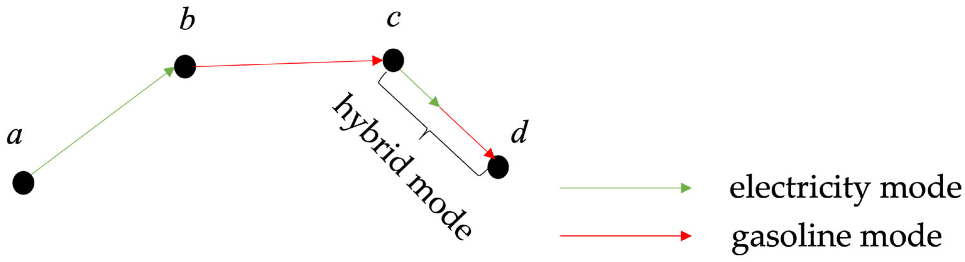
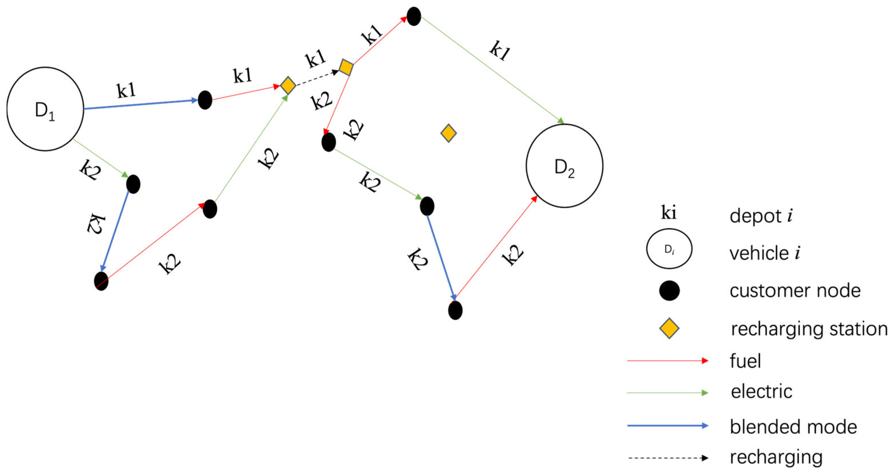
3.1. Problem Description

The Plug-in Hybrid Electric Vehicle Routing Problem (PHEVRP) is formulated on a complete graph G = (V, E). The vertex set V consists of an origin depot O, a destination depot D, a set of customers C = {v₁, v₂,…v_n}, and a set of recharging stations F = {f₁, f₂,…f_s}. Each edge in the set E, connecting any two vertices i, j ∈ V, has an associated distance d_i,j and travel time t_i,j.

A fleet of homogeneous PHEVs is assigned to distribute freight, each potentially undertaking a route visiting a subset of customers, departing from and returning to designated depots. Each customer i ∈ C has an associated demand ω_i and a predefined time window [r_i, l_i], within which service must commence. Vehicles arriving before or after these windows must wait or reschedule accordingly.

Each PHEV can operate in three modes: electric, gasoline, or hybrid mode, with hybrid mode allowing flexible switching between electricity and gasoline. Vehicles have uniform load capacity Z, battery capacity Q, and gasoline tank capacity Π. Partial recharging is allowed at recharging stations with a charging rate θ, and recharge time depends on the difference between battery levels upon arrival and departure. Since the fuel driving range significantly exceeds that of electric power in freight operations, refueling is not explicitly modeled in this study.

The primary objective of the PHEVRP is minimizing total operational costs, including vehicle investment costs, driver time costs, energy consumption expenses (fuel and electricity), and recharging expenses. Decision variables involve selecting routes and customer sequences for each PHEV, scheduling departures at each node, determining the energy usage proportions (gasoline, electric, or hybrid) for each arc, and managing battery recharge levels at stations. The hybrid mode cost for traversing an arc (i,j) is defined as follows:

$$cos{t}_{ij}=P_{i,j}^k{d}_{i,j}+F_{i,j}^k{d}_{i,j}$$

(1)

Here, $P_{i,j}^k$ denotes the proportion of distance covered by vehicle k using the electric mode on arc (i,j), while $F_{i,j}^k$ represents the corresponding proportion using the fuel mode, satisfying $P_{i,j}^k+F_{i,j}^k=1$. Figure 1 illustrates an example scenario of the described PHEVRP.

The proposed PHEVRP includes time window constraints (PHEVRP-TW), where each customer can have multiple disjoint time windows. A vehicle arriving between time windows must wait until the next available window begins. To make it clearer, Figure 2 illustrates an example of the PHEVRP.

For simplicity, we make the following assumptions:

• Fleet Consistency: Only one type of PHEV is used in the distribution.
• Linear Charging Behavior: The charging process is assumed to be linear, meaning that the amount of energy replenished is directly proportional to the charging time.

3.2. Formulation

The mathematical formulation involves a set of parameters and decision variables, which are summarized in

Table 2. Parameters and decision variables used in the model.

Parameters:
$O$	The set of origin node (depot) $v_0$
$C$	The set of customer nodes, $C \{v_1, v_2,... v_n\}$ , totally n customers
$D$	The set of destination node (the depot) $v_{n+1}$
$F$	The set of charging station node, $F=\{f_1, f_2,... f_s\}$ , totally s available charging stations
$m$	Total number of available vehicles
$K$	The set of vehicles, $K=\{p_1, p_2,... p_m\}$
$d_{ij}$	Distances between node i and j
$t_{ij}$	Travel time between node i and j
$T_{max}$	Maximum travel time for the route
${\epsilon }_i$	Service time at customer node i
${\omega }_i$	Demand at customer node i
[$r_i$ , li]	Time window limit for serving the customer i (i$\in$ I)
$e_i^k$	The remaining battery level for vehicle k that arrival at node i
$q_i^k$	The remaining battery level for vehicle k that departs node i
$u_i^k$	The remaining gasoline level for vehicle k that arrival at node i
${\lambda }_e$	The consumption rate of battery per distance
${\lambda }_f$	The consumption rate of gasoline per distance
$\theta$	Recharging rate
$Q$	Battery capacity for the vehicle
$\Pi$	Gasoline tank capacity for the vehicle
$Z$	Maximum load of commodity for the vehicle
${\sigma }_1$	The cost for vehicles travel time (i.e., salary for drivers)
${\sigma }_2$	The cost for charging at charging station
${\sigma }_3$	The cost for using a vehicle per day
${\sigma }_4$	The cost for using battery per distance
${\sigma }_5$	The cost for using gasoline per distance
Decision variable
$x_{i,j}^k$	Binary variable equal to 1 if a vehicle travels from node i to j and 0 otherwise
${\tau }_i^k$	Departure time for vehicle k at node i
$P_{i,j}^k$	The portion of distance for vehicle k passing through arc (i, j) with the electric mode activated
$F_{i,j}^k$	The proportion of distance for vehicle k passing through arc (i, j) with the fuel mode activated

.

We present the formulation, starting with the objective function.

$$\begin{gathered} min {\sigma }_1{\sum }_{k\in K}{\sum }_{i\in O\cup C\cup F}{\sum }_{j\in C\cup F\cup D|i\ne j}{x}_{i,j}^k t_{i,j} \\ {+\sigma }_2\sum _{k\in K}\sum _{i\in F}(q_i^k-e_i^k) \\ {+\sigma }_3\sum _{k\in K}\sum _{j\in C\cup F}{x}_{v_0 ,j}^k \\ {+\sigma }_4\sum _{k\in K}\sum _{i\in O\cup C\cup F}\sum _{j\in C\cup F\cup D|i\ne j}{P}_{i,j}^k{d}_{i,j} \\ {+\sigma }_5\sum _{k\in K}\sum _{i\in O\cup C\cup F}\sum _{j\in C\cup F\cup D|i\ne j}{F}_{i,j}^k{d}_{i,j} \end{gathered}$$

(2)

The objective function (2) includes five parts: time cost, charging cost, vehicle cost, electric consumption cost, and fuel consumption cost.

$$\sum _{k\in K}\sum _{i\in O\cup C\cup F}\sum _{j\in C\cup F\cup D|i\ne j}{x}_{i,j}^k=1 , \forall i\in C$$

(3)

$$\sum _{j\in C\cup D|i\ne j}{x}_{i,j}^k\le 1, \begin{array}{c}\forall i\in O\cup F\hfill \\ \forall k\in K\hfill \end{array}$$

(4)

$$\sum _{i\in O\cup C\cup F|i\ne j}{x}_{i,j}^k=\sum _{i\in C\cup F\cup D|i\ne j}{x}_{j,i}^k, \begin{array}{c}\forall j\in C\cup F,j\ne i\hfill \\ \forall k\in K\hfill \end{array}$$

(5)

$$1\le \sum _{k\in K}\sum _{j\in C\cup F\cup D}{x}_{v_0 ,j}^k\le m,$$

(6)

$$1\le \sum _{k\in K}\sum _{j\in O\cup C\cup F}{x}_{j ,v_{n+1}}^k\le m,$$

(7)

$${\tau }_i^k+\left(t_{i,j}+{\epsilon }_i\right)x_{i,j}^k-T_{max}\left(1-x_{i,j}^k\right)\le {\tau }_j^k, \begin{array}{c}\forall k\in K\hfill \\ \forall i\in O\cup C\hfill \\ \forall j\in C\cup F\cup D,j\ne i\hfill \end{array}$$

(8)

$${\tau }_i^k+t_{i,j}{x}_{i,j}^k+\theta (q_i^k-e_i^k)-{(T}_{max}+\theta Q)\left(1-x_{i,j}^k\right)\le {\tau }_j^k, \begin{array}{c}\forall k\in K\hfill \\ \forall i\in F\hfill \\ \forall j\in C\cup F\cup D,j\ne i\hfill \end{array}$$

(9)

$${r_i\le \tau }_i^k\le l_i, \begin{array}{c}\forall k\in K\hfill \\ \forall i\in C\hfill \end{array}$$

(10)

$$\sum _{i\in O\cup C\cup F}\sum _{j\in C\cup F\cup D|i\ne j}{{\omega }_{i}x}_{i,j}^k\le Z, \forall k\in K$$

(11)

$$0\le e_j^k\le e_i^k-{\lambda }_e{P}_{i,j}^k{d}_{i,j}+Q\left(1-x_{i,j}^k\right), \begin{array}{c}\forall k\in K\hfill \\ \forall i\in O\cup C\hfill \\ \forall j\in C\cup F\cup D,j\ne i\hfill \end{array}$$

(12)

$$0\le e_j^k\le q_i^k-{\lambda }_e{P}_{i,j}^k{d}_{i,j}+Q\left(1-x_{i,j}^k\right), \begin{array}{c}\forall k\in K\hfill \\ \forall i\in F\hfill \\ \forall j\in C\cup F\cup D,j\ne i\hfill \end{array}$$

(13)

$$0\le u_j^k\le u_i^k-{\lambda }_f{F}_{i,j}^k{d}_{i,j}+\Pi \left(1-x_{i,j}^k\right), \begin{array}{c}\forall k\in K\hfill \\ \forall i\in O\cup C\cup F\hfill \\ \forall j\in C\cup F\cup D,j\ne i\hfill \end{array}$$

(14)

$$P_{i,j}^k+F_{i,j}^k=x_{i,j}^k, \begin{array}{c}\forall k\in K\hfill \\ \forall i\in O\cup C\cup F\hfill \\ \forall j\in C\cup F\cup D,j\ne i\hfill \end{array}$$

(15)

Constraints (3) ensure that each customer is visited exactly once by exactly one vehicle. Constraints (4) restrict each depot and charging station to have at most one successor, preventing multiple visits by different vehicles. Constraints (5) enforce flow conservation, ensuring that the number of arcs entering and leaving each customer or charging station is balanced for every vehicle. Constraints (6) and (7) ensure that at least one and at most m vehicles depart from the origin depot and return to the destination depot, respectively. Constraints (8) and (9) enforce temporal consistency along the vehicle’s route but differ in the type of node they apply to and the components they include. Constraint (8) applies to customer or origin nodes and accounts for both travel time and service duration at the departure node. In contrast, Constraint (9) applies to charging stations, where no service time is considered, but the time required for partial battery recharging is included using the term $\theta (q_i^k-e_i^k)$. In both constraints, the binary variable $x_{i,j}^k$ functions as an activation switch: when arc (i, j) is traversed ($x_{i,j}^k=1$), the corresponding timing constraint is fully enforced; otherwise, it is relaxed by a sufficiently large penalty term—either $T_{max}$ or $T_{max}+\theta Q$—to preserve linearity.

Constraints (10) ensure arrival times at each customer node fall within their specified time windows. Constraints (11) enforce that each vehicle’s total load does not exceed its maximum capacity. Constraints (12) and (13) govern the evolution of battery energy levels throughout the vehicle’s route by distinguishing between arrival and departure battery states. Constraint (12) applies when a vehicle travels from a depot or customer node, where recharging is not allowed. In this case, the vehicle departs with the same battery level as when it arrived, i.e., $q_i^k=e_i^k$. The battery level at the next node j must be less than or equal to the departure level minus the energy consumed in electric mode, modeled as ${\lambda }_e P_{i,j}^k d_{i,j}$. In contrast, Constraint (13) applies at charging stations, where recharging is permitted. Upon arrival at node i, the vehicle has battery level $e_i^k$, and after recharging, it departs with a higher level $q_i^k\ge e_i^k$. The energy used to travel from node i to node j is then deducted from $q_i^k$ to determine the arrival battery level at j. The term $q_i^k-e_i^k$ thus represents the amount of energy charged at the station. To maintain linearity with respect to the binary routing variable $x_{i,j}^k$, a relaxation term $Q(1-x_{i,j}^k)$ is added, ensuring that the constraint is only enforced when the arc (i,j) is active.

Constraint (14) models the evolution of the fuel level as the vehicle traverses arc (i, j). Specifically, the fuel level upon arrival at node j must not exceed the departure fuel level $u_i^k$ minus the fuel consumed on that arc, calculated as ${\lambda }_f{F}_{i,j}^k d_{i,j}$, where $F_{i,j}^k$ denotes the proportion of the arc traveled in fuel mode. Similarly to the battery constraints, a relaxation term $\Pi (1-x_{i,j}^k)$ is included to maintain linearity with respect to the binary routing variable $x_{i,j}^k$. Constraint (15) directly links the energy mode proportions to the routing decision. It requires that the sum of the electric-mode and fuel-mode proportions equals the binary routing variable. This ensures that energy allocation is only defined for arcs that are actually traversed and is zero otherwise. The constraint provides a concise and effective way to integrate hybrid energy usage into the routing structure while preserving model linearity. The constraint elegantly integrates hybrid energy usage into the routing structure while preserving linearity.

Constraints (16)–(21) define bounds and integrality constraints for arrival times, battery and fuel levels, hybrid mode proportions, and routing decisions.

$$0\le {\tau }_i^k\le T_{max}, \begin{array}{c}\forall k\in K\hfill \\ \forall i\in O\cup C\cup F\cup D\hfill \end{array}$$

(16)

$$0\le e_i^k\le q_i^k\le Q, \begin{array}{c}\forall k\in K\hfill \\ \forall i\in O\cup C\cup F\cup D\hfill \end{array}$$

(17)

$$0\le u_i^k\le \Pi , \begin{array}{c}\forall k\in K\hfill \\ \forall i\in O\cup C\cup F\cup D\hfill \end{array}$$

(18)

$$0\le P_{ij}^k\le 1, \begin{array}{c}\forall k\in K\hfill \\ \forall i\in O\cup C\cup F\hfill \\ \forall j\in C\cup F\cup D,j\ne i\hfill \end{array}$$

(19)

$$0\le F_{ij}^k\le 1, \begin{array}{c}\forall k\in K\hfill \\ \forall i\in O\cup C\cup F\hfill \\ \forall j\in C\cup F\cup D,j\ne i\hfill \end{array}$$

(20)

$$x_{ij}^k\in \{\mathrm{0,1}\}, \begin{array}{c}\forall k\in K\hfill \\ \forall i\in O\cup C\cup F\hfill \\ \forall j\in C\cup F\cup D,j\ne i\hfill \end{array}$$

(21)

Constraints (15)–(19) represent the restrictions imposed on the variables.

This model can be solved directly by solver GUROBI 10.0 and the branch and cut algorithm is called. The algorithm complexity of this model is O ($N_v\ast 2^{N_v}$), and this growth rate is exponential. As such, the exact optimal solution in a reasonable execution time is limited only to small-size problems. Therefore, we provide an algorithm based on column generation to decompose the model into a path-based master problem and a sub-problem with a resource-constrained search path.

4. Decomposition-Based Algorithm for the PHEVRP

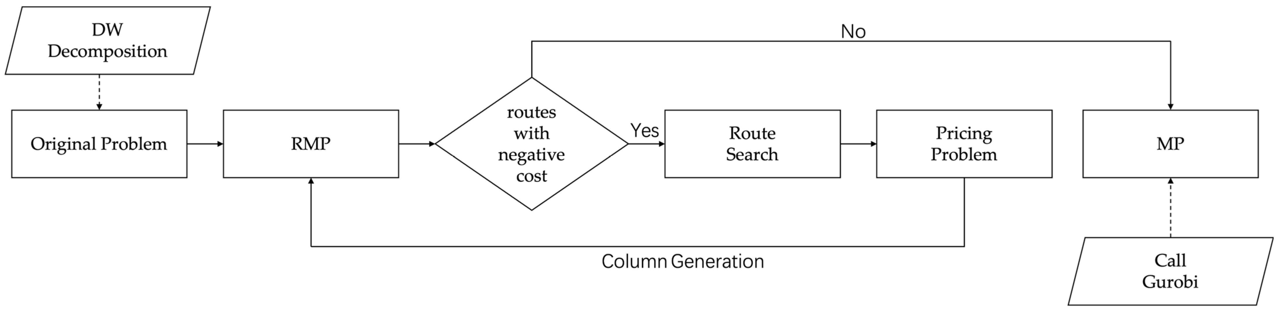
This formulation provides a compact and tractable to efficiently tackle large-scale instances of the Plug-in Hybrid Electric Vehicle Routing Problem (PHEVRP). This section introduces a decomposition-based algorithm utilizing Dantzig–Wolfe decomposition and column generation. This approach reformulates the original model into a Restricted Master Problem (RMP) and a Pricing Subproblem. The subproblem considers time window constraints and partial recharging dynamics, enabling flexible and efficient path generation strategies.

• Algorithm Overview
• Step 1: Apply Dantzig–Wolfe decomposition to divide the original problem into an RMP and a pricing subproblem.
• Step 2: Construct an initial feasible solution and add it to the RMP.
• Step 3: Solve the RMP to obtain dual variables and use them to guide the pricing subproblem. Add routes (columns) with negative reduced cost to the RMP.
• Step 4: If no more columns with negative reduced cost are found, proceed to Step 5; otherwise, return to Step 3.
• Step 5: Convert the continuous RMP into an Integer Master Problem (MP) by enforcing binary constraints.
• Step 6: Solve the MP to obtain the final optimal route combination.

This process is illustrated in Figure 3 and significantly improves scalability and solution quality under realistic operational constraints.

4.1. Path-Based Reformulation of the Restricted Master Problem (RMP)

The RMP selects an optimal combination of feasible routes that collectively satisfy coverage and resource constraints. The notations used are listed in

Table 3. Notations in the RMP formulation.

Sets:
${\Omega }_k$	Set of all feasible routes for vehicle k; $p\in {\Omega }_k$
$\Omega$	Set of all feasible routes across all vehicles
Variable
$x_{ij}^p$	1 if edge (i,j) is included in route p, 0 otherwise
$c^p$	Total cost of route p
$P_{ij}^p$	Proportion of electric energy used on edge (i,j) in route p
$F_{ij}^p$	Proportion of fuel energy used on edge (i,j) in route p
${\lambda }^p$	Selection weight (decision variable) for route p
$a_i^p$	Integer variable indicating whether node i is visited in route p

.

• Transformation and Constraints

Vehicle-level decisions are expressed using path-based variables:

$$x_{ij}^k=\sum _{p\in {\Omega }_k}{x}_{ij}^p{\lambda }^p \begin{array}{c}\forall k\in K\hfill \\ \forall i\in O\cup C\cup F\hfill \\ \forall j\in C\cup F\cup D,j\ne i\hfill \end{array}$$

(22)

$$P_{ij}^k=\sum _{p\in {\Omega }_k}{P}_{ij}^p{\lambda }^p\begin{array}{c}\forall k\in K\hfill \\ \forall i\in O\cup C\cup F\hfill \\ \forall j\in C\cup F\cup D,j\ne i\hfill \end{array}$$

(23)

$$F_{ij}^k=\sum _{p\in {\Omega }_k}{F}_{ij}^p{\lambda }^p\begin{array}{c}\forall k\in K\hfill \\ \forall i\in O\cup C\cup F\hfill \\ \forall j\in C\cup F\cup D,j\ne i\hfill \end{array}$$

(24)

$$F_{ij}^p+P_{ij}^p=1 \begin{array}{c}\forall p\in {\Omega }_k\hfill \\ \forall i\in O\cup C\cup F\hfill \\ \forall j\in C\cup F\cup D,j\ne i\hfill \end{array}$$

(25)

$$\sum _{p\in {\Omega }_k}{\lambda }^p=1$$

(26)

$${\lambda }^p\ge 0\forall p\in {\Omega }_k.$$

(27)

$$a_i^p=\sum _{j\in C\cup F\cup D|i\ne j}{x}_{ij}^p \begin{array}{c}\forall i\in O\cup C\cup F\hfill \\ \forall p\in {\Omega }_k\hfill \end{array}$$

(28)

Constraints (22)–(24) aggregate the routing variables, electric-mode proportions, and fuel-mode proportions of vehicle k over all its feasible paths. Constraint (25) ensures that for each arc used in any path, the proportions of electric and fuel modes sum to one, preserving the hybrid energy assignment structure. Constraint (26) enforces that each vehicle selects exactly one path, and (26) maintains non-negativity of the path-selection variables. Constraint (27) links the node visitation indicator $a_i^p$ with the arc usage within each path.

• Cost Calculation

The cost of each path p is precomputed as follows:

$$\begin{gathered} c^p={\sigma }_1\sum _{i\in O\cup C}\sum _{j\in C\cup D|i\ne j}\sum _{p\in {\Omega }_k}{t}_{ij}{x}_{ij}^p \\ {+\sigma }_2\sum _{i\in F}\sum _{p\in {\Omega }_k}\left(q_i-e_i\right)x_{ij}^p \\ {+\sigma }_4\sum _{i\in O\cup C\cup F}\sum _{j\in C\cup F\cup D|i\ne j}\sum _{p\in {\Omega }_k}{P}_{ij}^p{d}_{i,j} \\ {+\sigma }_5\sum _{i\in O\cup C\cup F}\sum _{j\in C\cup F\cup D|i\ne j}\sum _{p\in {\Omega }_k}{F}_{ij}^p{d}_{i,j} \end{gathered}$$

(29)

RMP Objective and Constraints

$$min\sum _{p\in \Omega }{c}^p{\lambda }^p$$

(30)

$$\sum _{p\in \Omega }{a}_i^p{\lambda }^p=1 \forall i\in C$$

(31)

$$\sum _{p\in \Omega }{a}_i^p{\lambda }^p\le 1 \forall i\in O\cup F\cup D$$

(32)

$$\sum _{p\in \Omega }{\lambda }^p\le m,$$

(33)

$${\lambda }^p\ge 0\forall p\in {\Omega }_k$$

(34)

The objective function (30) minimizes the total cost across all selected routes. Constraint (31) guarantees that each customer is visited exactly once, while (32) ensures that each depot or charging station is visited at most once. Constraint (33) limits the total number of vehicles dispatched, and (34) enforces non-negativity. This reformulation reduces problem complexity and enables efficient column generation. The generation of feasible paths p and the associated constraint handling are described in detail in the subsequent sections.

4.2. Heuristic Initialization via IMPACT-Based Node Insertion

This section introduces a construction strategy for generating initial solutions feasible paths p required in Section 3.2. We adopt the IMPACT [43] heuristic to determine the optimal insertion positions of customer nodes based on their cost impact on the existing route. The IMPACT score is computed using three key indicators:

• Insertion Slack (IS):

$$I{S}_v=r_v-({\tau }_i+t_{iv})$$

(35)

indicating the available slack time before servicing customer v when inserted after node i.

• Urgency Index (IU):

$$I{U}_v=\left({\displaystyle \frac{1}{\left|J\right|-1}}\right)\sum _{j\in J\backslash \left\{v\right\}} max\left\{\right(l_j-r_v-t_{vj}), (l_j-r_j-t_{vj}\left)\right\}$$

(36)

reflecting the average urgency of inserting customer v in relation to the remaining customer time windows.

Distance Increase (ID): represents the incremental travel cost from inserting customer v between two existing nodes.

Then the overall IMPACT score is as follows:

$$IMPACT=I{S}_v+I{U}_v-I{D}_v$$

(37)

The node with the highest IMPACT score is selected for insertion.

The detailed steps are as follows:

Step 1: Initialize the set of unassigned customer nodes J and an empty route set.

Step 2: For each vehicle, initialize a basic route starting from depot O and ending at depot D.

Step 3: For each unassigned customer $v\in J$, compute the IMPACT score using the formulas above.

Step 4: Insert the customer with the highest IMPACT score into its optimal position within the current route. Update the route set and remove the inserted customer from J. Repeat until all customers are assigned.

Illustrative Example.

Assume three unassigned customer nodes—$v_1$, $v_2$, and $v_3$—with the attributes shown in

Table 4. Example calculation of IMPACT scores for candidate customer insertions.

Customer	${\mathit{r}}_{\mathit{v}}$	${\mathit{t}}_{\mathit{i}\mathit{v}}$	$\mathit{I}{\mathit{S}}_{\mathit{v}}$	$\mathit{I}{\mathit{U}}_{\mathit{v}}$	$\mathit{I}{\mathit{D}}_{\mathit{v}}$	IMPACT Score
$v_1$	20	5	5	33	3	35
$v_2$	22	7	5	28	2	31
$v_3$	18	6	2	30	4	28

, when considered for insertion after node i with ${\tau }_i$ = 10. The corresponding Insertion Slack (IS), Urgency Index (IU), and Distance Increase (ID) values are calculated, and the IMPACT score for each candidate is derived using Equation (37). The node with the highest score is selected for insertion into the current route.

Based on the computed IMPACT scores, customer $v_1$ has the highest score (35) and is therefore selected for insertion at this step.

4.3. Pricing Subproblem: Resource-Constrained Shortest Path Model

To improve the RMP solution, the pricing subproblem identifies new routes with negative reduced cost.

4.3.1. Reduced-Cost Model

The objective of the pricing subproblem is to find a path p with minimized reduced cost $c^p$, computed by adjusting the original cost $c^p$ with the dual variables from the RMP:

$$min c^p$$

(38)

Subject to the following resource and time constraints:

$$\mathrm{s}.\mathrm{t}. {\tau }_i+\left(t_{i,j}+{\epsilon }_i\right)\le {\tau }_j, \begin{array}{c}\forall i\in (O\cup C)\hfill \\ \forall j\in (C\cup D) j\ne i\hfill \end{array}$$

(39)

$${\tau }_i+t_{i,j}+\theta \left(q_i-e_i\right)\le {\tau }_j,\begin{array}{c}\forall i\in F\hfill \\ \forall j\in (C\cup D) j\ne i\hfill \end{array}$$

(40)

$${r_i\le \tau }_i\le l_i, \forall i\in P$$

(41)

$$0\le e_j\le e_i-{\lambda }_e{P}_{i,j}{d}_{i,j}, \begin{array}{c}\forall i\in (O\cup C)\hfill \\ \forall j\in (C\cup D), j\ne i\hfill \end{array}$$

(42)

$$0\le e_j\le q_i-{\lambda }_e{P}_{i,j}{d}_{i,j}, \begin{array}{c}\forall i\in \left(F\right)\hfill \\ \forall j\in (C\cup D), j\ne i\hfill \end{array}$$

(43)

These constraints ensure time feasibility, respect battery consumption, and differentiate the vehicle’s behavior when departing from customer nodes versus charging stations.

4.3.2. Reduced-Cost Calculation

The reduced cost ${\overline{c}}^p$ for a candidate path p is calculated by adjusting the original path cost $c^p$ using dual variable values obtained from the restricted master problem:

$$min {\overline{c}}^p=c^p-\sum _{i\in C}{a}_i^p {\pi }_i-\sum _{j\in F}{a}_j^p{\varphi }_j$$

(44)

where

${\pi }_i$ and ${\varphi }_j$ are the dual values associated with the customer visit constraints and the charging station visitation constraints, respectively;

$a_i^p$ indicates whether node i is visited in path p;

The dual variables for the origin and destination depots are set to zero: ${\pi }_O={\pi }_D=0.$

4.3.3. Label-Correcting Algorithm for Path Generation

To solve the ESPPRC efficiently, we apply a label-correcting algorithm (Algorithm 1) adapted from Chabrier [6], which expands partial paths while maintaining feasibility. Each path is rep-resented by a label containing a set of resource attributes, as detailed in

Table 5. Labeling Formulation Notations.

Sets:
${\overline{c}}^p$	Reduced cost of path p
${\omega }^p$	Load consumed along path p
$u^p$	Fuel consumed along path p
${\tau }^p$	Arrival time at the current node
${\delta }^p$	Number of nodes unreachable from the current partial path
$V_i^p$	Binary: 1 if node $i\in C\cup F$ is unreachable Via path p; 0 otherwise

.

Dominance Rule

A path $p^{*}$ dominates another path p if both end at the same node and

$${\overline{c}}^{p^{*}}\le {\overline{c}}^p , {\omega }^{p^{*}}\le {\omega }^p, u^{p^{*}}\le u^p, {\delta }^{p^{*}}\le {\delta }^p, \forall i\in C\cup F$$

Only non-dominated labels are retained for further extension.

Algorithm 1: Label Extension Procedure
Input: (i, Lp, j)
Output: Lp*
1:  if (${\omega }^p+{\omega }_j>Z$) or ${(u}^p+{\sigma }_5{d}_{ij}$ > $\Pi$) or (${\tau }^p+t_{ij}+s_i>l_j$) then
2:	Lp* = Lp
3:  else
4:	Update ${\omega }^{p^{*}}$ , $u^{p^{*}}$ , ${\tau }^{p^{*}}$ and ${\overline{c}}^{p^{*}}$
5:	if $Lp* is not dominated:$
6:		$V_S^{p*}=V_S^p$
7:		${\delta }^{p*}={\delta }^p$
8:		if (j $\in C\cup F$ ) then
9:			${\delta }^{p*}$ = ${\delta }^{p*}$ +1
10:			$V_j^{p*}$ = 1
11:	for all t ∈ successors of j:
12:		if adding t violates load, fuel, or time window:
13:			${\delta }^{p*}$ = ${\delta }^{p*}$ +1
14:			$V_t^{p*}$ = 1

In this process, energy consumption and feasibility are updated at each extension. When a charging station is visited, full recharge is assumed to simplify the battery state update. This pricing subproblem formulation effectively identifies new routes for the RMP with negative reduced cost. By leveraging reduced-cost guidance and efficient label management, the subproblem enables the overall column generation framework to scale to large instances while maintaining feasibility and optimality across multiple resource dimensions.

4.4. Master Problem and Algorithm Pseudo-Code

After discretizing the decision variables in the RMP, the master problem is reformulated as Section 3.2. This transformation significantly reduces the variable space, making the problem tractable for commercial solvers. The complete formulation is as follows:

$$min\sum _{p\in \Omega }{c}^p{\lambda }^p{+\sigma }_3\sum _{p\in \Omega }{\lambda }^p$$

(45)

$$\sum _{p\in \Omega }{a}_i^p{\lambda }^p=1 \forall i\in C$$

(46)

$$\sum _{p\in \Omega }{a}_i^p{\lambda }^p\le 1 \forall i\in O\cup F\cup D$$

(47)

$$\sum _{p\in \Omega }{\lambda }^p\le m,$$

(48)

$${\lambda }^p\in \left\{\mathrm{0,1}\right\},\forall p\in \Omega$$

(49)

This compact mixed-integer formulation serves as the final step in the column genera-tion framework and ensures that an optimal set of routes is selected. To solve the PHEVRP efficiently, the Algorithm 2 outlines the Dantzig–Wolfe Decomposition Algorithm that combines restricted master problem optimization with iterative column generation.

Algorithm 2: Dantzig–Wolfe Decomposition
Input: Original PHEVRP instance data
Output: Optimal route combination and energy mode strategy
1:  Generate initial feasible paths Ω0 using heuristic (see Section 4.2);
2:  Initialize the Restricted Master Problem (RMP) with the initial path set (see Section 4.3.1)
3:  Repeat (Column Generation Loop)
4:	Solve RMP (Relaxed version) to obtain dual variables πi and φj (see Section 4.3.2)
5:	Solve Pricing Subproblem using Label-Correcting Algorithm (see Section 4.3.3)
6:	If a path p negative reduced cost c̅p < 0 is found, add it to Ω
7:  Until no more columns with negative reduced cost are identified;
8:  Convert the relaxed RMP into the final Integer Master Problem (MP);
9:	Fix λp ∈ {0,1} in RMP
10:	Solve the MP as a mixed-integer program to determine the optimal route set.

5. Numerical Experiments

5.1. Experimental Setup and Parameter Configuration

This section provides a detailed explanation of the data assumptions and sources. The vehicle-related data used in this study is inherited from Li et al. [42].

Table 6. Vehicle parameter settings.

Parameter	Value
Battery capacity (Q)	10.5 kWh
Electricity consumption rate (${\lambda }_e$ )	0.5 kWh/mile
Electricity cost (${\sigma }_3$ )	USD 0.12/kWh
Fuel tank capacity ($\Pi$ )	25 gallons
Fuel consumption rate (${\lambda }_f$ )	17.7 m/g
Fuel cost (${\sigma }_4$ )	USD 4.18/gal

summarizes the key vehicle parameters employed in the model, which are representative of typical plug-in hybrid electric vehicle (PHEV) specifications. These parameters include energy capacities, consumption rates, and corresponding unit costs for both electricity and fuel. The time cost is estimated based on the average monthly wage in Shanghai, divided by the standard monthly working hours, resulting in a rate of USD 6.94 per hour. Similarly, the electricity cost is assumed to be USD 0.17 per kilowatt-hour (kWh). The computational instances are derived from the well-known Solomon benchmark suite [44], in which instances are categorized into three types based on customer distribution:

• C-type: clustered customer locations;
• R-type: randomly distributed customers;
• RC-type: a combination of R-type and C-type distributions.

Each original instance contains 100 nodes. Smaller-scale instances are generated by extracting the first 10 to 50 customers from the original datasets. While instances of the same type and size share similar structures, they may differ in their time window settings. For example, both C1_10 and C2_10 are C-type instances with 10 nodes each, but they differ in the configuration of their time windows.

The implementation of the proposed approach is carried out in Spyder 5.5.1 using Python 3.12, with Gurobi 10.0 used as the optimization solver.

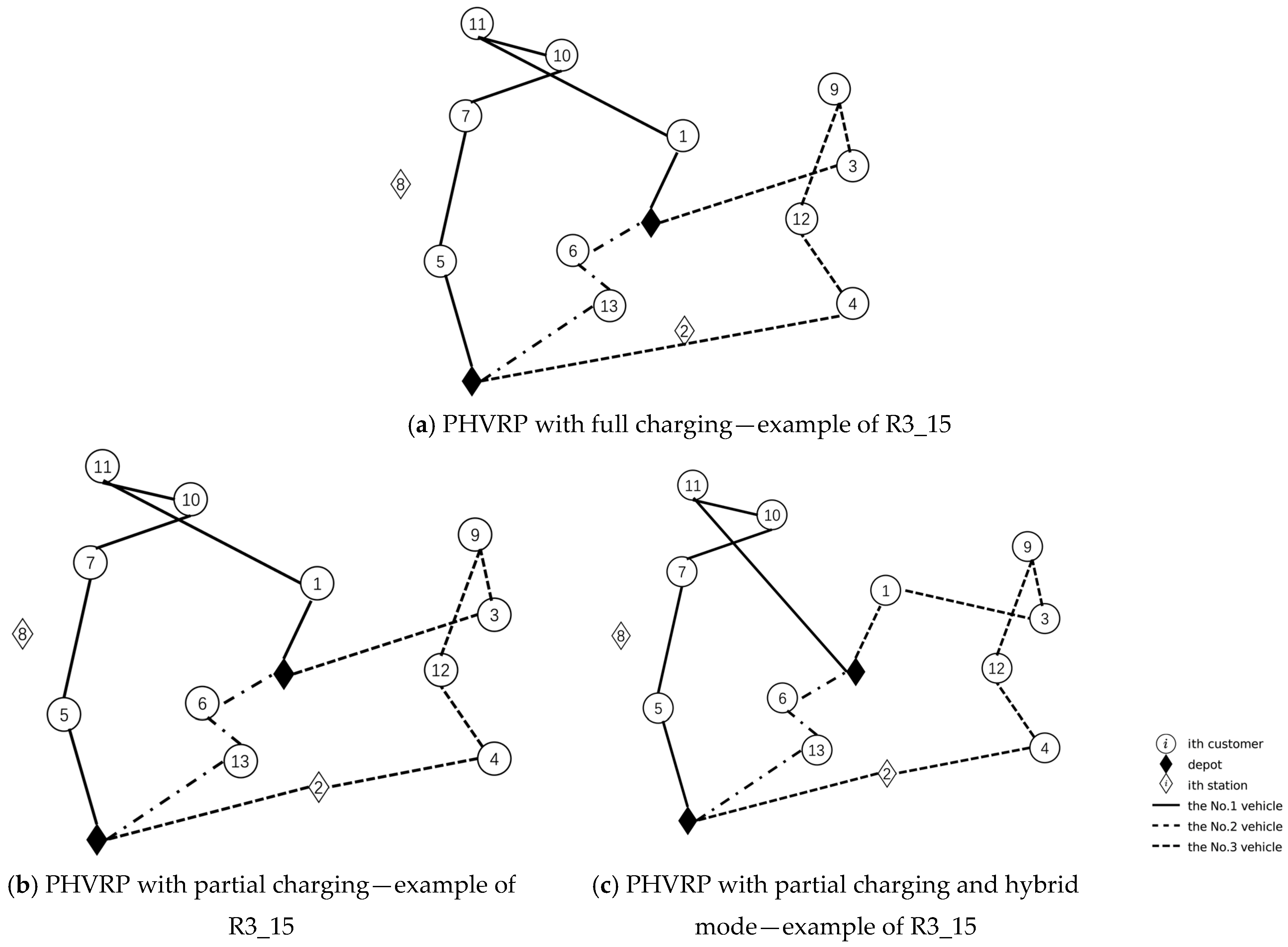
5.2. Cost Advantages of Partial Charging and Hybrid Mode

This section evaluates the cost-saving benefits of employing partial charging and hybrid mode (denoted as PHVRP–Partial Charging and Hybrid Mode) in the PHEVRP, compared with two alternative strategies: full charging only (PHVRP–Full Charging) and partial charging only (PHVRP–Partial Charging). To conduct this comparison, the variable P_ij in the model is set as a binary variable, thereby disabling hybrid mode. Full charging is enforced by adding Constraint (50) to the model:

$$q_j\ge Q{x}_{i,j}^k, \begin{array}{c}\forall k\in K\hfill \\ \forall i\in O\cup C\cup F\hfill \\ \forall j\in F,j\ne i\hfill \end{array}$$

(50)

To clearly demonstrate the advantages of the hybrid approach, we analyze benchmark instances of various customer types, ranging from 10 to 50 nodes.

To clearly illustrate the differences, Figure 4 compares the cost variations among three strategies—PHVRP with full recharging, PHVRP with partial recharging, and PHVRP with partial recharging and hybrid mode—under different customer distribution types. All values in the figure are non-negative, indicating that both partial recharging and hybrid strategies consistently outperform the full recharging strategy in terms of cost savings. This confirms the effectiveness of these approaches in reducing overall logistics costs. The detailed analysis is as follows:

C-type Instances:

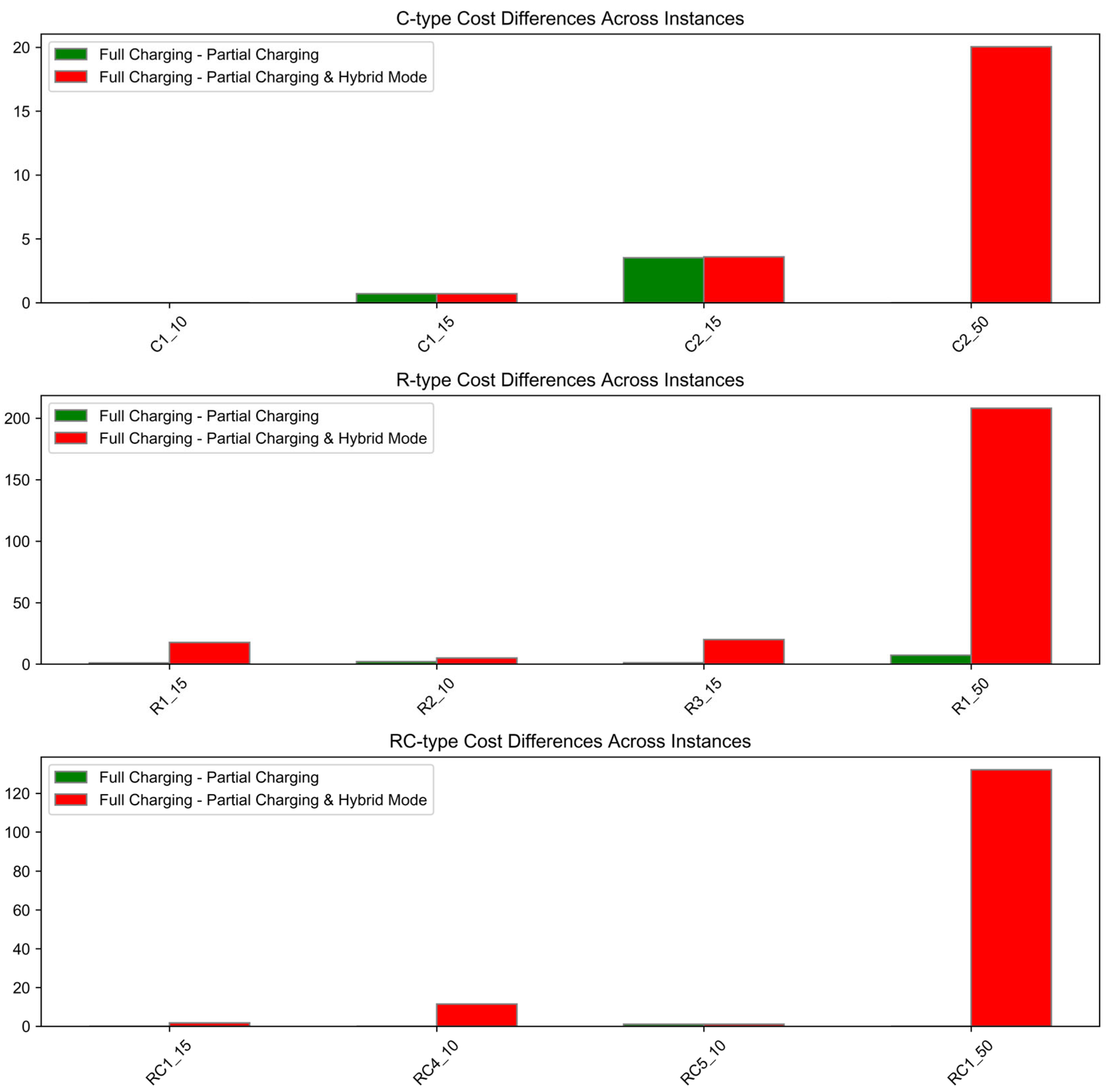
• For most C-type instances (e.g., C1_10, C1_15), the costs across all three strategies—full charging, partial charging, and hybrid mode—are nearly identical. This suggests that when customers are geographically clustered and the instance size is small, the choice of energy strategy has a minimal impact on cost.
• An exception is C2_50, where the hybrid mode reduces the cost by approximately 20 units, indicating that in larger clustered instances, energy-mode flexibility can yield meaningful cost improvements.

R-type Instances:

• Significant cost reductions are observed under the hybrid mode. In particular, R1_50 and R3_15 achieve savings of 208 and 19.9 units, respectively.
• These findings suggest that when customer locations are dispersed, and routing becomes more complex, allowing partial charging or enabling hybrid mode significantly enhances route feasibility and cost efficiency.
• Even in smaller instances such as R2_10, moderate savings are observed, indicating that random distributions benefit from flexible energy strategies regardless of scale.

RC-type Instances:

• In most small-scale RC-type instances (e.g., RC1_15, RC5_10), the cost differences across strategies are relatively small.
• However, for larger instances like RC1_50, the hybrid mode achieves a cost saving of 132 units, demonstrating that energy flexibility becomes increasingly valuable in mixed-distribution scenarios as instance size increases.

In conclusion, the cost-saving advantage of partial recharging and hybrid mode becomes more pronounced as problem size grows—especially in random and mixed distribution scenarios. When customer locations are clustered, flexible energy strategies remain beneficial, but their impact is more limited unless the instance size is large enough to require complex route and energy planning.

To further investigate the underlying causes of cost differences among the three strategies, this section also examines charging time and fuel consumption, which are critical operational factors. Given that electricity is generally much cheaper than gasoline, analyzing these two aspects helps clarify the cost-effectiveness of each strategy. The results show that across a wide range of scenarios (with 10 to 50 customer nodes), the three strategies exhibit notable differences in both charging time and fuel consumption. Figure 5 illustrates these differences by comparing the charging time and fuel consumption under full charging, partial charging, and partial charging and hybrid strategies across various customer distributions. The bar charts are divided into different groups of scenarios—specifically, smaller-scale instances with 10 to 15 customer nodes and larger-scale instances with 15 to 50 customer nodes—providing a clearer view of how strategy performance scales with problem size.

From the perspective of charging time, the full charging strategy results in zero charging time in most scenarios. This is because full recharging is often incompatible with strict time window constraints, limiting its flexibility in practical applications. In contrast, the partial charging and hybrid mode shows slightly longer charging times than the pure partial charging strategy. This phenomenon is due to the greater flexibility of the hybrid approach, which allows vehicles to access more charging stations, thereby increasing charging opportunities.

Regarding fuel consumption, the partial charging and hybrid mode typically achieves a lower fuel usage by optimizing the energy mix between gasoline and electricity. This results in cost reductions in most cases. The benefit comes not only from reduced fuel usage but also from improved electric energy utilization efficiency as charging time increases.

Beyond energy usage strategies, the choice of routing is also affected by different charging strategies. Compared to PHVRP with full charging, PHVRP with partial charging tends to detour to reach charging stations, which can naturally increase travel costs. However, the partial charging and hybrid mode allows the vehicle to use fuel as a supplement to electricity, thus avoiding unnecessary detours to reach a charging station.

Taking instance R3_15 as an example, Figure 6 illustrates the routing differences under three strategies. Scenarios (a), (b), and (c) represent PHVRP with full charging, PHVRP with partial charging, and PHVRP with partial charging and hybrid mode, respectively.

In Scenario (a), vehicles are constrained to full recharging only, which significantly limits routing flexibility. As a result, instead of taking a long detour to Charging Station 2 for a full charge, the vehicle opts to use gasoline directly to reach distant customers such as Node 11. This decision reflects a cost-based trade-off: although gasoline is typically more expensive per unit of energy, avoiding long detours can lead to lower total route costs. Consequently, no charging station is visited in this scenario, and the vehicle relies solely on fuel to maintain feasibility and minimize operational costs.

In Scenario (b), partial charging is permitted, offering more flexibility. The vehicle chooses to visit Charging Station 2, as only a limited amount of energy is needed to complete the route. This enables a more efficient routing strategy that avoids excessive detours, demonstrating how partial charging can reduce route length and improve operational efficiency.

However, Scenario (c) introduces a hybrid mode, enabling the vehicle to dynamically switch between electricity and fuel. This significantly improves routing flexibility. Compared to Scenario (b), the route changes from (Depot → Node 11) to (Depot → Node 1 → Node 11). This change occurs because, in (b), the vehicle cannot reach Node 11 directly due to limited battery energy and thus requires a detour to recharge. In contrast, under the hybrid strategy in (c), the vehicle travels from the depot to Node 1 using electricity and then switches to fuel to reach Node 11. This avoids the need to visit a charging station solely for completing the leg to Node 11.

Moreover, the hybrid mode enables a more balanced task allocation between vehicles. In Scenario (c), the second vehicle follows the route (Depot → Node 1 → Node 3), which is shorter than the (Depot → Node 1 → Node 11) path taken by the first vehicle. This allocation reduces overall travel distance and improves energy efficiency, highlighting the hybrid mode’s advantage in optimizing both routing feasibility and total cost.

In summary, the hybrid mode combined with partial charging demonstrates significant advantages in improving electric energy utilization and reducing reliance on fuel consumption. In the long run, this contributes to lowering overall operational costs. Therefore, the following sections focus exclusively on analyzing the PHEVRP model under the hybrid mode with partial charging strategy.

5.3. Cost Sensitivity Analysis

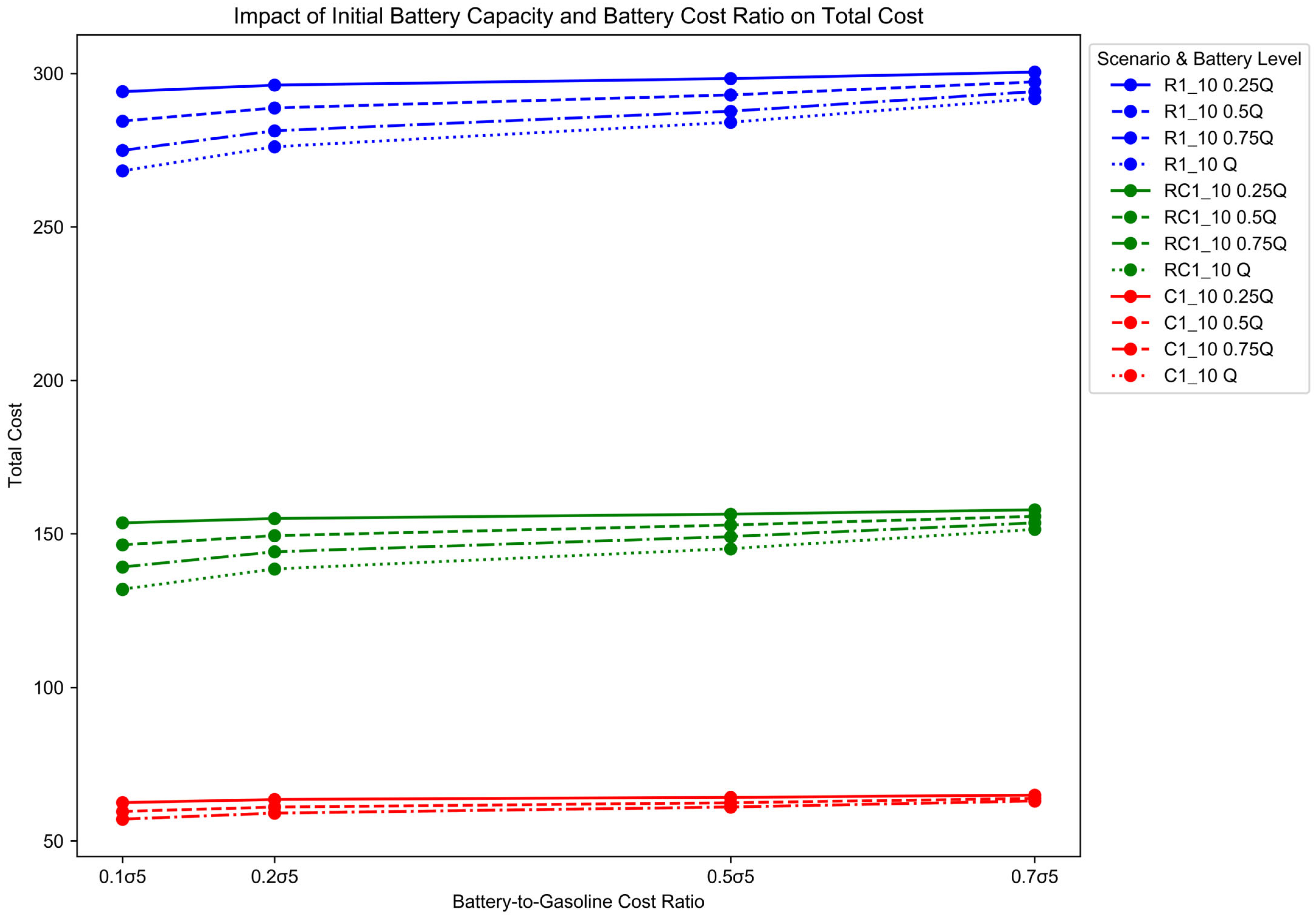
5.3.1. Influence of Initial Battery Capacity and Battery-to-Gasoline Cost Ratio on Total Cost

This section builds upon the superior performance demonstrated by the PHVRP–Partial Charging and Hybrid Mode and further investigates how variations in key cost-related parameters affect total cost. Specifically, we explore the influence of initial battery capacity (IBC) and the battery-to-gasoline cost ratio (BGR) across different scenario types.

We consider four levels of IBC (0.25Q, 0.5Q, 0.75Q, and Q) and four BGR values (0.1σ₅, 0.3σ₅, 0.5σ₅, and 0.7σ₅) and apply these to three benchmark instances: C1_10, R1_10, and R2_10. These scenarios represent different customer distributions, providing a robust basis for sensitivity analysis.

Figure 6 illustrates the changes in total cost across three benchmark scenarios (C1_10, R1_10, and R2_10) under different combinations of initial battery capacity (0.25Q to Q) and battery-to-gasoline cost ratios (0.1σ₅ to 0.7σ₅). The results demonstrate that increasing battery capacity reduces cost, while a higher battery cost ratio increases total cost, with greater sensitivity observed in R-type instances.

As illustrated in Figure 7, several important trends can be observed:

• Impact of IBC:

Increasing the battery capacity significantly reduces total cost across all tested scenarios. This is primarily because larger capacities reduce the need for frequent recharging and diminish fuel dependency.

• Impact of BGR:

Higher BGR values are associated with increased total costs. This reflects the operational burden introduced by expensive batteries, even when they reduce fuel usage.

• Sensitivity Differences by Scenario Type:

The sensitivity to BGR and IBC varies by instance. R-type scenarios are more cost-sensitive than C-type, likely due to their dispersed customer locations, which require longer travel and more frequent energy replenishment.

In addition to total cost, we analyze the interaction between individual cost components, including travel time cost, charging cost, vehicle cost, battery cost, and fuel cost. These relationships are visualized in Figure 8, with key observations summarized below:

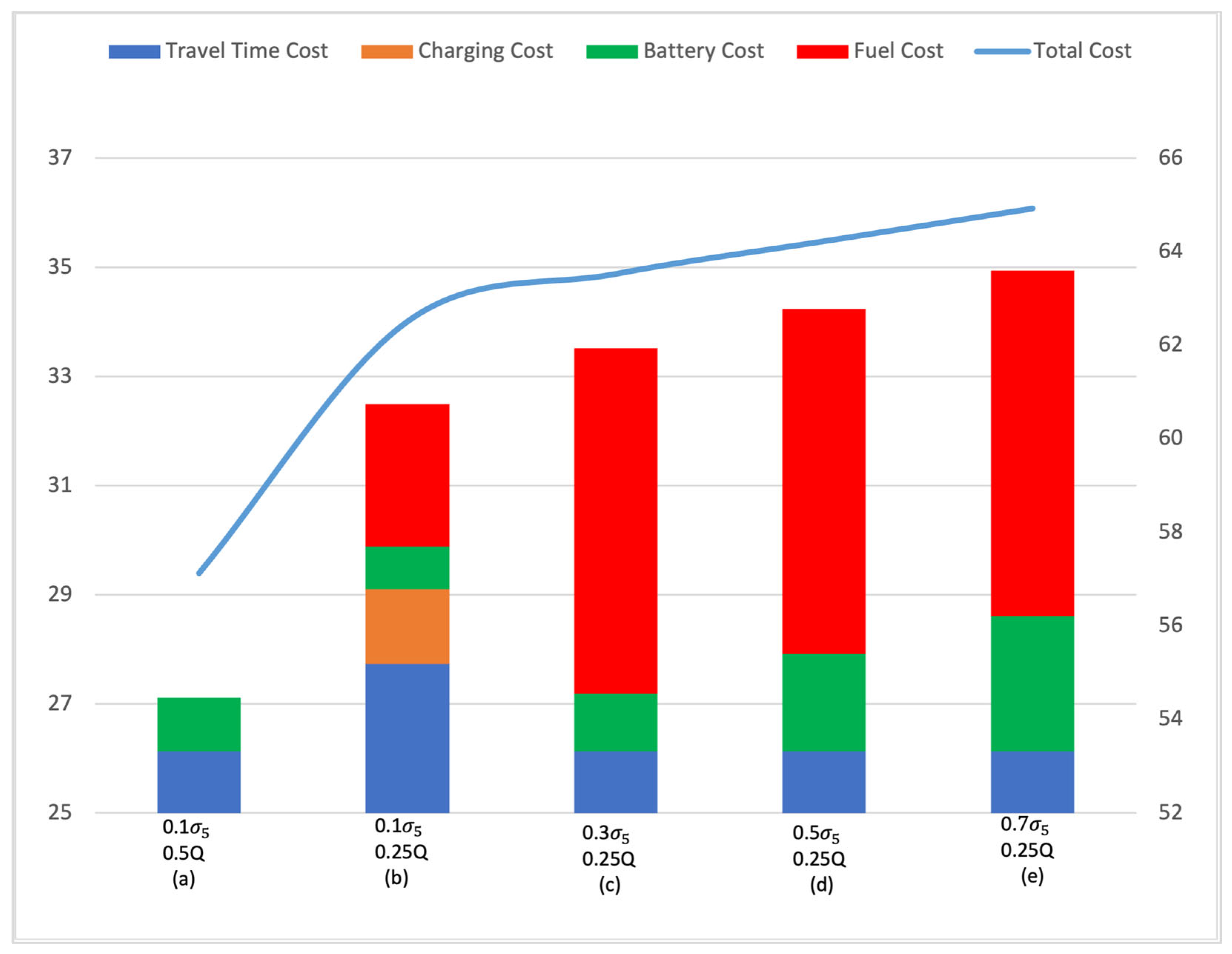
• Travel Time vs. Charging Cost:

In scenarios (a) and (c), where the BGR is held constant, but IBC varies (Q vs. 0.75Q), travel time costs remain largely unchanged. This suggests that when battery capacity sufficiently supports the trip, routing decisions dominate travel time rather than battery-related limitations.

• Charging Cost with Low IBC:

In scenario (b), a low IBC (0.25Q) results in elevated charging costs. This is likely due to more frequent charging requirements or detours to reach available charging stations.

• Battery vs. Fuel Trade-Off:

In scenarios (d) and (e), total cost increases as BGR rises from 0.5σ₅ to 0.7σ₅. Although higher battery use reduces gasoline consumption, the increase in battery cost may outweigh the savings—especially under high battery price conditions.

Implications and Practical Insights

These findings highlight the importance of carefully balancing battery capacity and cost in hybrid electric vehicle routing. While higher battery capacity offers operational advantages, its cost must be economically justified, particularly in large-scale logistics operations. The results also provide strategic insight for fleet managers and policymakers when designing cost-effective energy strategies for plug-in hybrid vehicle deployment.

5.3.2. Sensitivity Analysis of Charging Price at Charging Stations

In this section, we examine how fluctuations in charging prices affect routing decisions and total cost. Inspired by real-world observations from Shanghai [45]—where electricity prices at charging stations vary across regions and time periods—we conduct a sensitivity analysis on the electricity cost parameter ${\sigma }_2$, testing three levels: 1.5${\sigma }_2$, 2.0${\sigma }_2$, and 2.5${\sigma }_2$. These values represent low, standard, and high charging cost scenarios, respectively. As noted in Section 5.3.1, clustered customers (C-type) typically do not require recharging due to short route distances, while randomly distributed customers (R-type) tend to avoid recharging because of costly detours. Thus, we select a representative RC-type instance for this analysis, offering a balanced scenario in which recharging decisions are both necessary and sensitive to cost variations.

Figure 9 illustrates the impact of ${\sigma }_2$ variations on the two cost components that exhibit meaningful changes: time cost and charging cost. The blue dashed line represents the charging cost, while the red dashed line indicates the time cost. As observed, when the charging price increases to 2.5${\sigma }_2$, the charging cost drops sharply to zero. This suggests that vehicles avoid recharging altogether under high electricity prices, opting instead to rely solely on fuel in order to minimize overall costs. For lower charging prices, the charging cost increases linearly, reflecting more frequent or larger recharges.

Interestingly, the time cost—defined here as travel time only and excluding any recharging duration—also exhibits a slight decrease when 2.5${\sigma }_2$. This reduction stems from the vehicle’s strategic avoidance of detours to charging stations, thereby shortening the total path distance. In contrast, the time cost remains steady at approximately 123.13 in lower charging price scenarios, where recharging is still economically favorable and detours are taken.

These findings confirm the economic interplay between electricity price and routing efficiency: under peak charging prices, PHEVs may abandon recharging and switch to gasoline use, resulting in a lower time cost but potentially higher fuel usage. This highlights the importance of dynamic pricing policies and their influence on route planning strategies in hybrid vehicle operations.

5.4. Performance Evaluation of Dantzig–Wolfe Decomposition

This section evaluates the performance of the DW (Dantzig–Wolfe) decomposition algorithm relative to the full optimization model. To provide a comparative benchmark, an Ant Colony Optimization (ACO) algorithm [46] is introduced, incorporating the exact evaluation model from Section 4.3.1 and the reduced cost computation from Section 4.3.2. The complete pseudocode and relevant parameters are provided in Appendix A.

Table 7. Performance comparison among the full model, Dantzig–Wolfe decomposition (DW), and ant colony optimization (ACO).

Instance	Model		Dantzig–Wolfe Decomposition			Ant Colony Optimization
	Objective	CPU (s)	Objective	CPU (s)	Gap1 (%)	Objective	CPU (s)	Gap2 (%)	Gap3 (%)
C1_15	155.30	1305.40	155.30	418.60	0	155.30	1591.30	0
C1_25	227.54	9162.10	234.30	1147.30	3	268.40	4383.10	18	15
R1_15	406.12	1121.60	406.12	84.44	0	415.91	2910.80	2	2
R1_25	844.14	33,031.75	850.10	160.20	1	866.80	5715.20	3	2
R2_15	341.80	42,463.53	344.56	258.40	1	378.13	1679.50	11	10
RC1_25	763.75	5535.12	763.75	104.60	0	834.39	4267.10	9	9
C1_30	/	/	335.30	3826.80	/	413.16	5421.16	/	23
C2_25	/	/	285.48	8515.80	/	344.87	4837.84	/	21
C2_30	/	/	595.30	7568.10	/	682.64	5849.80	/	15
C3_25	/	/	500.59	15,087.10	/	523.79	5349.67	/	5
C3_30	/	/	672.70	28,031.75	/	758.76	6637.16	/	13
R1_30	/	/	960.17	121.10	/	1110.58	7846.10	/	16
R1_50	/	/	1617.40	303.30	/	2223.52	12,924.40	/	37
R1_100	/	/	2177.51	2647.80	/	3301.90	28,678.60	/	52
R2_25	/	/	761.03	457.70	/	880.53	6555.20	/	16
R2_30	/	/	819.76	1721.06	/	901.10	8618.30	/	10
R2_50	/	/	1558.60	5082.52	/	1876.20	13,540.60	/	20
RC1_50	/	/	1574.27	506.96	/	1949.10	9685.10	/	24
R2_100	/	/	2298.20	37,031.80	/	3034.10	27,051.32	/	32
R1_200	/	/	7656.44	110,013.16	/	15,004.23	52,689.7	/	95

Gap1 = (DW Objective − Model Objective)/Model Objective; Gap2 = (ACO Objective − Model Objective)/Model Objective; Gap3 = (ACO Objective − DW Objective)/DW Objective. C-type: clustered customer distribution; R-type: random; RC-type: mixed. R1_200 is from the Homberger and Gehring benchmark to represent large-scale case.

compares the computational performance of the optimization model, the DW decomposition algorithm, and the ACO heuristic across a series of benchmark instances. These instances vary in terms of customer distribution types—Clustered (C-type), Random (R-type), and Mixed (RC-type)—as well as problem sizes, ranging from 15 to 100 customer nodes. Additionally, to demonstrate scalability in large-scale settings, one instance from the widely used Homberger [21] and Gehring dataset (200 customers) is also included. The table reports the total objective value and CPU time (in seconds) required by each method. For instances where the model failed to return a solution within a reasonable time, the result is marked as “/”.

Three gap metrics are used to assess relative performance:

• Gap1 = (DW Objective − Model Objective)/Model Objective;
• Gap2 = (ACO Objective − Model Objective)/Model Objective;
• Gap3 = (ACO Objective − DW Objective)/DW Objective.

Based on the results presented in Table 7, the analysis can be divided into the following aspects:

• Solution Quality Comparison

The DW decomposition algorithm consistently delivers high-quality solutions. For smaller instances such as C1_15, R1_15, and RC1_25, DW achieves exact matches with the full model (Gap1 = 0%). In most other solvable cases, the gap remains within 1–3%, such as C1_25 (3%), R1_25 (1%), and R2_15 (1%). These results highlight the algorithm’s ability to accurately approximate optimal solutions by effectively capturing route structures through reduced-cost-driven subproblem solving, even when the full model becomes computationally intractable.

In contrast, the ACO heuristic exhibits a noticeable drop in solution quality as the problem scale or complexity increases. While it performs adequately on small instances, its objective values diverge more significantly in medium to large cases. For example, C1_25 shows a 15% gap relative to DW, and R2_15 has a 10% deviation. The deterioration becomes pronounced in larger instances, such as C1_30 (23%), R1_50 (37%), R1_100 (52%), and R1_200 (95%). This reflects ACO’s limitations in exploiting dual information or systematically pruning the search space, which is essential for high-precision solutions.

2.

Computational Efficiency and Time Stability

In terms of computational efficiency, ACO clearly outperforms DW in both speed and stability, particularly in large-scale instances. For instance, in R2_15, DW takes over 42,000 s, whereas ACO completes in 1679 s. In the large-scale cases R2_100 and R1_200, DW requires over 37,000 and 110,000 s, respectively, while ACO delivers results within 27,000 and 52,000 s.

However, DW is still competitive in small and moderately structured problems. In R1_15 and RC1_25, DW completes in just 84 and 104 s, respectively—faster than ACO. The overall runtime instability of DW stems from its dependency on iteratively solving complex pricing subproblems and updating the master problem. When numerous negative reduced cost columns are needed for convergence, or when energy constraints lead to a sparse feasible space, DW’s performance deteriorates sharply.

3.

Instance Type and Size Effects

• Clustered Instances (C-type): These are generally easier for both methods due to geographical compactness. Nevertheless, ACO still yields large errors in bigger instances, e.g., C1_30 (23%) and C2_25 (21%).
• Random Instances (R-type): These present the most difficulty due to spatial dispersion and complex routing paths. DW retains reasonable accuracy, but its runtime becomes significantly longer (e.g., R2_15: 42,463 s; R2_100: 37,000 s). In contrast, ACO remains fast but shows sharp declines in solution quality—e.g., R1_50 (37%), R1_100 (52%), R1_200 (95%).
• Mixed Instances (RC-type): These have intermediate difficulty. ACO produces moderate gaps (e.g., RC1_50: 24%), while DW maintains accuracy as long as runtime remains within practical limits.

To further evaluate DW’s performance, Figure 10 presents boxplots comparing the full optimization model and the Dantzig–Wolfe (DW) decomposition algorithm across six small-scale benchmark instances (C1_15, C1_25, R1_15, R1_25, R2_15, and RC1_25), with a focus on objective values (left panel) and CPU time (right panel).

From the left panel, the boxplots show that the median objective values of DW nearly coincide with those of the full model, reflecting strong alignment in solution quality. The interquartile range (IQR) of DW is narrow across all cases, indicating high stability and consistency in solution quality. Moreover, DW exhibits no extreme outliers in objective values, and in instances like R1_15 and RC1_25, it achieves the same optimal value as the full model. In cases such as C1_25 and R1_25, the mild overestimation is minimal—within 3%—confirming DW’s ability to accurately capture optimal routing structures.

In the right panel, the boxplots of CPU time reveal a striking computational advantage for DW. The median runtimes for DW are all under 300 s, while those for the full model extend up to tens of thousands of seconds—most notably in R2_15, where the full model exceeds 40,000 s. The upper whiskers and outliers in the model’s runtime distribution further emphasize its volatility and inefficiency in larger problem settings. By contrast, DW’s runtime distribution is tightly bounded with fewer extreme values, showcasing improved computational stability and scalability.

Figure 11 presents boxplots comparing the DW decomposition algorithm and the ACO heuristic across 20 benchmark instances in terms of objective value (left panel) and CPU time (right panel).

In the left panel, DW consistently achieves lower median objective values than ACO across nearly all instances, indicating superior solution quality. The IQR of DW is also noticeably tighter, reflecting more stable performance with less variability. In contrast, ACO displays a much wider IQR and numerous extreme outliers, especially in large-scale cases like R1_100, R2_100, and R1_200, where its objective values are significantly higher—sometimes exceeding DW by more than 50%. This suggests that ACO frequently deviates from near-optimal solutions when the problem becomes more complex.

The right panel compares CPU times. Although DW exhibits some runtime dispersion, including long upper whiskers and a few prominent outliers (e.g., C3_30, R2_100, and R1_200), it still achieves faster average computation times than ACO in most small- to medium-sized instances. This demonstrates DW’s overall computational advantage, especially when the problem structure is conducive to efficient column generation. In contrast, while ACO shows more compact runtime distributions with fewer outliers—attributable to its metaheuristic nature—it often requires more time than DW in structured instances like C1_15, R1_15, and RC1_25. Thus, despite occasional volatility, DW generally offers superior speed-performance trade-offs, making it a more effective choice when both accuracy and efficiency are important.

In summary, the DW decomposition algorithm consistently delivers high-precision solutions, with optimality gaps typically below 3%, even for medium-scale instances. Its ability to leverage reduced-cost pricing ensures reliable performance where exactness matters. Although DW’s runtime may fluctuate due to the complexity of column generation, it is often faster than ACO in small to mid-sized cases. In contrast, ACO, while computationally stable, generally produces less accurate solutions and requires more time in many instances. Overall, DW offers a better balance of quality and efficiency, making it the preferred choice when accuracy is prioritized.

6. Conclusions

This study proposed a PHEV routing model that incorporates partial charging and hybrid energy mode switching. The hybrid strategy effectively reduces fuel consumption and detours for recharging, thereby lowering operational costs—particularly in clustered customer scenarios. Given the computational complexity of the model, especially in instances involving more than 30 customers, a Dantzig–Wolfe (DW) decomposition algorithm was introduced to efficiently narrow the solution space and enable the solution of large-scale problems where exact methods become impractical.

Experimental results demonstrate that, from a modeling perspective, the proposed hybrid-mode and partial charging strategy significantly outperforms traditional full-charging and single-mode approaches, especially in clustered customer scenarios, by improving energy flexibility and reducing overall operational costs. From an algorithmic standpoint, the DW decomposition algorithm consistently delivers high-accuracy solutions with optimality gaps typically below 3% and achieves faster computation than the ACO heuristic in most structured instances. While ACO shows more stable runtimes, it often yields inferior solution quality.

Despite the promising results, this study has several limitations. The current model assumes static traffic conditions and unlimited charging station capacity, without considering queuing delays or real-time network dynamics. Additionally, the DW algorithm, while effective, may suffer from computational instability in complex instances due to the variability of reduced-cost column generation.

Future research may focus on two directions. From a modeling perspective, integrating real-time traffic conditions, charging station congestion, and capacity constraints could enhance the model’s realism. From an algorithmic perspective, improving the stability of the DW algorithm through adaptive pricing strategies or hybridizing it with metaheuristics like ACO may further improve scalability while preserving solution quality for large and dynamic routing scenarios.

References

1. International Energy Agency. Tracking Clean Energy Progress 2023. Available online: https://www.iea.org/reports/tracking-clean-energy-progress-2023 (accessed on 13 February 2025).
2. UPS. Doing Good Is Good for Business. Available online: https://about.ups.com/us/en/our-impact/sustainability/sustainable-services/2022-ups-sustainability-report-.html (accessed on 13 February 2025).
3. Dantzig, G.B.; Ramser, J.H. The Truck Dispatching Problem. Manag. Sci. 1959, 6, 80–91. [Google Scholar] [CrossRef]
4. Nejad, M.M.; Mashayekhy, L.; Grosu, D.; Chinnam, R.B. Optimal Routing for Plug-In Hybrid Electric Vehicles. Transp. Sci. 2017, 51, 1031–1386. [Google Scholar] [CrossRef]
5. Bahrami, S.; Nourinejad, M.; Amirjamshidi, G.; Roorda, M.J. The Plugin Hybrid Electric Vehicle Routing Problem: A Power-Management Strategy Model. Transp. Res. Part C Emerg. Technol. 2020, 111, 318–333. [Google Scholar] [CrossRef]
6. Chabrier, A. Vehicle Routing Problem with Elementary Shortest Path Based Column Generation. Comput. Oper. Res. 2006, 33, 2972–2990. [Google Scholar] [CrossRef]
7. Lee, G.; Lee, J.S.; Park, K.S. Battery Swapping, Vehicle Rebalancing, and Staff Routing for Electric Scooter Sharing Systems. Transp. Res. Part E Logist. Transp. Rev. 2024, 186, 103540. [Google Scholar] [CrossRef]
8. Trotta, A.; Andreagiovanni, F.D.; Di Felice, M.; Natalizio, E.; Chowdhury, K.R. When UAVs Ride a Bus: Towards Energy-Efficient City-Scale Video Surveillance. In Proceedings of the IEEE INFOCOM 2018—IEEE Conference on Computer Communications, Honolulu, HI, USA, 15–19 April 2018. [Google Scholar] [CrossRef]
9. Kim, G. Electric Vehicle Routing Problem with States of Charging Stations. Sustainability 2024, 16, 3439. [Google Scholar] [CrossRef]
10. Longo, H.; Poggi de Aragão, M.; Uchoa, E. Solving Capacitated Arc Routing Problems Using a Transformation to the CVRP. Comput. Oper. Res. 2006, 33, 1823–1837. [Google Scholar] [CrossRef]
11. Fang, C.; Cai, Y.; Wu, Y. A Discrete Wild Horse Optimizer for Capacitated Vehicle Routing Problem. Sci. Rep. 2024, 14, 21277. [Google Scholar] [CrossRef]
12. Desrochers, M.; Desrosiers, J.; Solomon, M.M. A New Optimization Algorithm for the Vehicle Routing Problem with Time Windows. Oper. Res. 1992, 40, 342–354. [Google Scholar] [CrossRef]
13. Saksuriya, P.; Likasiri, C. Vehicle Routing Problem with Time Windows to Minimize Total Completion Time in Home Healthcare Systems. Mathematics 2023, 11, 4846. [Google Scholar] [CrossRef]
14. Balakrishnan, N. Simple Heuristics for the Vehicle Routeing Problem with Soft Time Windows. J. Oper. Res. Soc. 1993, 44, 279–287. [Google Scholar] [CrossRef]
15. Demir, E.; Bektaş, T.; Laporte, G. An Adaptive Large Neighborhood Search Heuristic for the Pollution-Routing Problem. Eur. J. Oper. Res. 2012, 223, 346–359. [Google Scholar] [CrossRef]
16. Lysgaard, J.; Letchford, A.N.; Eglese, R.W. A New Branch-and-Cut Algorithm for the Capacitated Vehicle Routing Problem. Math. Program. 2004, 100, 423–445. [Google Scholar] [CrossRef]
17. Baldacci, R.; Christofides, N.; Mingozzi, A. An Exact Algorithm for the Vehicle Routing Problem Based on the Set Partitioning Formulation with Additional Cuts. Math. Program. 2008, 115, 351–385. [Google Scholar] [CrossRef]
18. Xia, Y.; Zeng, W.; Zhang, C.; Yang, H. A Branch-and-Price-and-Cut Algorithm for the Vehicle Routing Problem with Load-Dependent Drones. Transp. Res. Part B Methodol. 2023, 171, 80–110. [Google Scholar] [CrossRef]
19. Baker, B.M.; Ayechew, M.A. A Genetic Algorithm for the Vehicle Routing Problem. Comput. Oper. Res. 2003, 30, 787–800. [Google Scholar] [CrossRef]
20. Cordeau, J.F.; Laporte, G.; Mercier, A. A Unified Tabu Search Heuristic for Vehicle Routing Problems with Time Windows. J. Oper. Res. Soc. 2001, 52, 928–936. [Google Scholar] [CrossRef]
21. Homberger, J.; Gehring, H. A Two-Phase Hybrid Metaheuristic for the Vehicle Routing Problem with Time Windows. Eur. J. Oper. Res. 2005, 162, 220–238. [Google Scholar] [CrossRef]
22. Altabeeb, A.M.; Mohsen, A.M.; Ghallab, A. An Improved Hybrid Firefly Algorithm for Capacitated Vehicle Routing Problem. Appl. Soft Comput. 2019, 84, 105728. [Google Scholar] [CrossRef]
23. Passias, A.; Sirakoulis, G.C. Comparative Study of Metaheuristic Algorithms for the Vehicle Routing Problem with Application to Recycling Waste Management. Parallel Process. Lett. 2025, 35, 2250001. [Google Scholar] [CrossRef]
24. Erdoğan, S.; Miller-Hooks, E. A Green Vehicle Routing Problem. Transp. Res. Part E Logist. Transp. Rev. 2012, 48, 100–114. [Google Scholar] [CrossRef]
25. Schneider, M.; Stenger, A.; Goeke, D. The Electric Vehicle-Routing Problem with Time Windows and Recharging Stations. Transp. Sci. 2014, 48, 500–520. [Google Scholar] [CrossRef]
26. Felipe, Á.; Ortuño, M.T.; Righini, G.; Tirado, G. A Heuristic Approach for the Green Vehicle Routing Problem with Multiple Technologies and Partial Recharges. Transp. Res. Part E Logist. Transp. Rev. 2014, 71, 111–128. [Google Scholar] [CrossRef]
27. Schiffer, M.; Walther, G. The Electric Location Routing Problem with Time Windows and Partial Recharging. Eur. J. Oper. Res. 2017, 260, 995–1013. [Google Scholar] [CrossRef]
28. Goeke, D.; Schneider, M. Routing a Mixed Fleet of Electric and Conventional Vehicles. Eur. J. Oper. Res. 2015, 245, 81–99. [Google Scholar] [CrossRef]
29. Macrina, G.; Di Puglia Pugliese, L.; Guerriero, F.; Laporte, G. The Green Mixed Fleet Vehicle Routing Problem with Partial Battery Recharging and Time Windows. Comput. Oper. Res. 2019, 101, 183–199. [Google Scholar] [CrossRef]
30. Du, S.; Li, S.; Han, H.; Qiao, J. Diversity-Based Niche Genetic Algorithm for Bi-Objective Mixed Fleet Vehicle Routing Problem with Time Window. Neural Comput. Appl. 2025, 37, 11479–11499. [Google Scholar] [CrossRef]
31. Rahmanifar, G.; Mohammadi, M.; Hajiaghaei-Keshteli, M.; Colombaroni, C.; Fusco, G.; Gholian-Jouybari, F. Two-Echelon Electric Vehicle Routing Problem with Battery Swap Stations on Real Network. IFAC-Pap. Online 2024, 58, 46–51. [Google Scholar] [CrossRef]
32. Desaulniers, G.; Errico, F.; Irnich, S.; Schneider, M. Exact Algorithms for Electric Vehicle-Routing Problems with Time Windows. Oper. Res. 2016, 64, 1388–1405. [Google Scholar] [CrossRef]
33. Keskin, M.; Çatay, B. Partial Recharge Strategies for the Electric Vehicle Routing Problem with Time Windows. Transp. Res. Part C Emerg. Technol. 2016, 65, 111–127. [Google Scholar] [CrossRef]
34. Gil-Gala, F.J.; Đurasević, M.; Jakobović, D. Evolving Routing Policies for Electric Vehicles by Means of Genetic Programming. Appl. Intell. 2024, 54, 12391–12419. [Google Scholar] [CrossRef]
35. Wei, X.; Niu, C.; Zhao, L.; Wang, Y. Combination of Ant Colony and Student Psychology-Based Optimization for the Multi-Depot Electric Vehicle Routing Problem with Time Windows. Clust. Comput. 2025, 28, 99. [Google Scholar] [CrossRef]
36. Raykin, L.; Roorda, M.J.; MacLean, H.L. Impacts of Driving Patterns on Tank-to-Wheel Energy Use of Plug-In Hybrid Electric Vehicles. Transp. Res. D Transp. Environ. 2012, 17, 243–250. [Google Scholar] [CrossRef]
37. Arslan, O.; Yıldız, B.; Kara¸san, O.E. Minimum Cost Path Problem for Plug-in Hybrid Electric Vehicles. Transp. Res. Part E Logist. Transp. Rev. 2015, 80, 123–141. [Google Scholar] [CrossRef]
38. Murakami, K. Formulation and Algorithms for Route Planning Problem of Plug-In Hybrid Electric Vehicles. Oper. Res. Int. J. 2018, 18, 497–519. [Google Scholar] [CrossRef]
39. Murakami, K. A New Model and Approach to Electric and Diesel-Powered Vehicle Routing. Transp. Res. Part E Logist. Transp. Rev. 2017, 107, 23–37. [Google Scholar] [CrossRef]
40. Wu, F.; Adulyasak, Y.; Cordeau, J. Modeling and Solving the Traveling Salesman Problem with Speed Optimization for a Plug-In Hybrid Electric Vehicle. Transp. Sci. 2024, 58, 562–577. [Google Scholar] [CrossRef]
41. Yu, V.F.; Redi, A.A.N.P.; Hidayat, Y.A.; Wibowo, O.J. A Simulated Annealing Heuristic for the Hybrid Vehicle Routing Problem. Appl. Soft Comput. 2017, 53, 119–132. [Google Scholar] [CrossRef]
42. Li, X.; Shi, X.; Zhao, Y.; Liang, H.; Dong, Y. SVND Enhanced Metaheuristic for Plug-In Hybrid Electric Vehicle Routing Problem. Appl. Sci. 2020, 10, 441. [Google Scholar] [CrossRef]
43. Ioannou, G.; Kritikos, M.; Prastacos, G. A Greedy Look-Ahead Heuristic for the Vehicle Routing Problem with Time Windows. J. Oper. Res. Soc. 2001, 52, 523–537. [Google Scholar] [CrossRef]
44. Solomon, M.M. Algorithms for the Vehicle Routing and Scheduling Problems with Time Window Constraints. Oper. Res. 1987, 35, 254–265. [Google Scholar] [CrossRef]
45. Liu, Z.; Zhou, Y.; Feng, D.; Xu, S.; Yi, Y.; Li, H.; Wang, H. Dynamic Pricing of Electric Vehicle Charging Station Alliances under Information Asymmetry. CSEE J. Power Energy Syst. 2025, 1–12, in press. [Google Scholar] [CrossRef]
46. Fan, L. A Two-Stage Hybrid Ant Colony Algorithm for the Multi-Depot Half-Open Time-Dependent Electric Vehicle Routing Problem. Complex Intell. Syst. 2024, 10, 2107–2128. [Google Scholar] [CrossRef]
Figure 1. An example segment used in energy mode analysis.
Mathematics 13 02239 g001
Figure 2. The figure provides an illustrative example of the described PHEVRP scenario.
Mathematics 13 02239 g002
Figure 3. Flowchart of the algorithm.
Mathematics 13 02239 g003
Figure 4. Cost differences by customer type.
Mathematics 13 02239 g004
Figure 5. Comparison of charging time and fuel consumption under different charging strategies across customer scenarios.
Mathematics 13 02239 g005
Figure 6. Routing path comparison under full charging, partial charging, and hybrid strategies in instance R3_15.
Mathematics 13 02239 g006
Figure 7. Impact of initial battery capacity and battery cost ratio on total cost.
Mathematics 13 02239 g007
Figure 8. Component-wise cost breakdown under varying battery capacities and cost ratios.
Mathematics 13 02239 g008
Figure 9. Cost breakdown at different charging price levels.
Mathematics 13 02239 g009
Figure 10. Performance comparison between the model and DW decomposition algorithm. Red line = median; circles = outliers.
Mathematics 13 02239 g010
Figure 11. Performance comparison between DW decomposition algorithm and the ant colony optimization. Red line = median; circles = outliers.
Mathematics 13 02239 g011