1. Introduction
Frequent sweeping is crucial for maintaining the cleanliness and overall quality of outdoor spaces such as parks [
1]. However, traditional sweeping methods, which are labor-intensive, face significant challenges, including labor shortages and concerns about worker health and safety. Robots are increasingly being deployed to address these issues to meet cleaning demands in public outdoor environments [
2,
3,
4].
For a cleaning robot to operate effectively, it requires a navigation system capable of generating paths that cover a surface completely while minimizing overlap. This process is known as Coverage Path Planning (CPP). Numerous approaches have been developed to address this problem [
5,
6]. For example, Song et al. [
7] proposed a method based on an exploratory Turing machine, which offers efficiency and guarantees full coverage. Nature-inspired algorithms have also emerged as a promising direction. For example, Kumar et al. [
8] proposed a CPP algorithm inspired by the way grass spreads over land. Another study [
9] introduced a Glasius bioinspired neural network to solve CPP tasks. Reinforcement Learning (RL) has demonstrated strong potential even for self-reconfigurable robots, which introduce significant dynamic constraints for CPP [
10].
The effectiveness of a CPP method often depends on multiple performance criteria, such as coverage rate, energy consumption, operation time, computational efficiency, and safety. The robot’s operating environment significantly influences these criteria; indoor settings require a properly integrated navigation system for confined spaces, which necessitates accurate localization, obstacle avoidance in narrow passages, and reliable performance under structured layouts. In contrast, outdoor environments require robust performance under varying terrain, lighting, and weather conditions that could cause localization degradation and make it difficult for the perception sensors array to perform appropriately. Optimization techniques such as Genetic Algorithms (GAs) have been used to develop energy-efficient CPP strategies for mobile robots [
11]. Multi-objective optimization methods further extend this by balancing several performance metrics simultaneously, such as maximizing coverage while minimizing energy use [
12]. The paper cited in [
13] used RL to improve robot safety while maintaining adequate coverage. Another work [
14] proposed a CPP approach that reduces coverage time by enabling adaptive size variation in the robot.
CPP algorithms are computationally expensive, as they must continuously track previously visited locations to identify new target areas. The complexity of CPP in large-scale environments is intrinsically tied to the nature of the algorithms; most are iterative and rely on cost functions to assign priority levels to different areas on a grid map [
15,
16]. While multi-threading can be used to improve computational efficiency to some extent [
17,
18], these methods still consume considerable time and system resources to complete the task. To reduce this computational burden, some approaches employ cell decomposition, in which the environment is divided into smaller regions based on obstacle geometry—a process known as decomposition. Dividing a large area into smaller, more manageable subregions is often more computationally feasible than attempting to cover the entire space as a whole [
19]. Galceran et al. [
20] analyzed trapezoidal and boustrophedon decomposition strategies and concluded that the trapezoidal method offers stronger guarantees for complete coverage.
More recently, Voronoi diagrams have gained attention in robotics, especially for target planning tasks across various applications [
21]. These diagrams help partition the environment in a way that supports both efficient coverage and collision avoidance. Even when the trapezoidal approach provides good results in practice, the method behaves better in small indoor environments. Whether outdoor environments are empty or full of obstacles, the objective of using Voronoi is to always provide a segmentation of the area, no matter if there are no obstacles. As discussed by Chee Sheng et al. [
22], some heuristic algorithms can also address coverage planning challenges with low computational overhead. For example, Yehoshua et al. [
23] proposed the spanning tree adversarial Coverage algorithm, which uses a layered approach to classify grid cells as safe, dangerous, or disconnected. The method prioritizes safe cells, connects disconnected cells through an optimal path, and finally groups and traverses the dangerous cells in a defined sequence. Depth-first search has also proven effective in large environments, mainly when partitioning the workspace. In such cases, the decomposition can be modeled as a graph or tree structure to ensure systematic coverage [
24]. Additionally, Rosa et al. [
25] proposed a Dijkstra-based algorithm that employs a swarm of robots to cover expansive areas while avoiding inter-robot collisions.
Reconfigurable modular robots and cooperative multi-robot teams have continued to boost coverage performance by dynamically reshaping their morphology [
14] and distributing workload [
25], respectively, which accelerates coverage. However, use of reconfigurable mechanisms and multi-robot systems with the capability to handle large cleaning payloads demanded by outdoor sweeping are expensive. Furthermore, irregular ground profiles, drifting localization in GPS-denied zones, weather exposure, and moving obstacles complicate real-time coordination and jeopardize uniform coverage, as recent field trials with MAVs and ground cleaners have exposed [
26,
27]. Consequently, many deployments still favor robust single-robot solutions fine-tuned for harsh terrain over large, communication-heavy fleets or reconfigurable robots.
Different CPP methods have their own merits and limitations [
22,
28]. Therefore, selecting an appropriate CPP method for a specific task, such as outdoor sweeping, can be challenging. We propose a novel CPP framework tailored for outdoor sweeping robots to address this. In this framework, CPP algorithms are treated as system modular components that can be replaced based on performance and task-specific requirements. The framework also incorporates both Voronoi- and grid-based clustering algorithms to discretize the environment and define target regions for the CPP algorithms. Target sorting is formulated as a Traveling Salesman Problem (TSP), which considers both obstacles and inter-cluster distances to determine an energy-efficient task execution order. Three different optimization methods are analyzed to solve the TSP. The proposed strategy follows the following workflow:
- (1)
Determine the traversable area from a large Point Cloud Library (PCL) map.
- (2)
Divide the area into smaller regions.
- (3)
Finding visiting sequence for subregions prioritizing energy efficiency (using TSP).
- (4)
Asynchronously generate coverage paths for each subregions.
- (5)
In parallel, enqueue each generated path into a task list for execution.
- (6)
Trigger the robot’s cleaning action to begin with the first item in the task list, while coverage paths for the remaining areas continue to be generated in the background.
This approach ensures that the robot remains active as early and continuously as possible by quickly assigning a target. The purpose of this approach is to establish a framework for outdoor robots that allows for the flexibility of switching maps and minimizing human involvement as much as possible in cleaning a target area. The comparison and analysis of coverage performance across different decomposition strategies and TSP methods in the context of outdoor sweeping of large environments are also key contributions of the paper. Importantly, the framework is platform-agnostic and developed on top of the Robot Operating System (ROS). Integration with various robotic platforms is straightforward, as platform-specific physical constraints are managed within the CPP algorithm implementation to maximize operational efficiency.
The rest of the paper is organized follows.
Section 2 presents the outdoor robot platform used for validating the proposed CPP framework. The proposed CPP framework is detailed in
Section 3.
Section 4 presents the simulation and robot hardware experiments and results. Conclusions of the work are given in
Section 5.
2. Robot Platform
We used the Panthera outdoor sweeping robot to implement the proposed CPP framework. The mechanical capabilities and software architecture of the Panthera robot are explained here to provide a clear understanding of the platform.
Figure 1 illustrates the hardware features of the robot, which includes two frontal brushes and a vacuum system connected to a set of brushes located at the bottom of the robot. The robot employs a differential drive locomotion system, with two main wheels positioned at the rear, a caster wheel at the front, and four servomotors used to raise and lower the frontal brushes and the trash bin.
The robot’s perception and computer vision systems include an Ouster-128 LiDAR (Ouster Inc., San Francisco, CA, USA) mounted on top for mapping and localization, and two Ouster-32 LiDARs for obstacle detection, enabling the definition of exclusion zones for safety. A Global Positioning System (GPS) further supports localization. Additionally, a depth camera is used for computer vision tasks such as obstacle identification, human detection, and signal recognition. A beacon light is also integrated to increase awareness of the autonomous unit among nearby pedestrians.
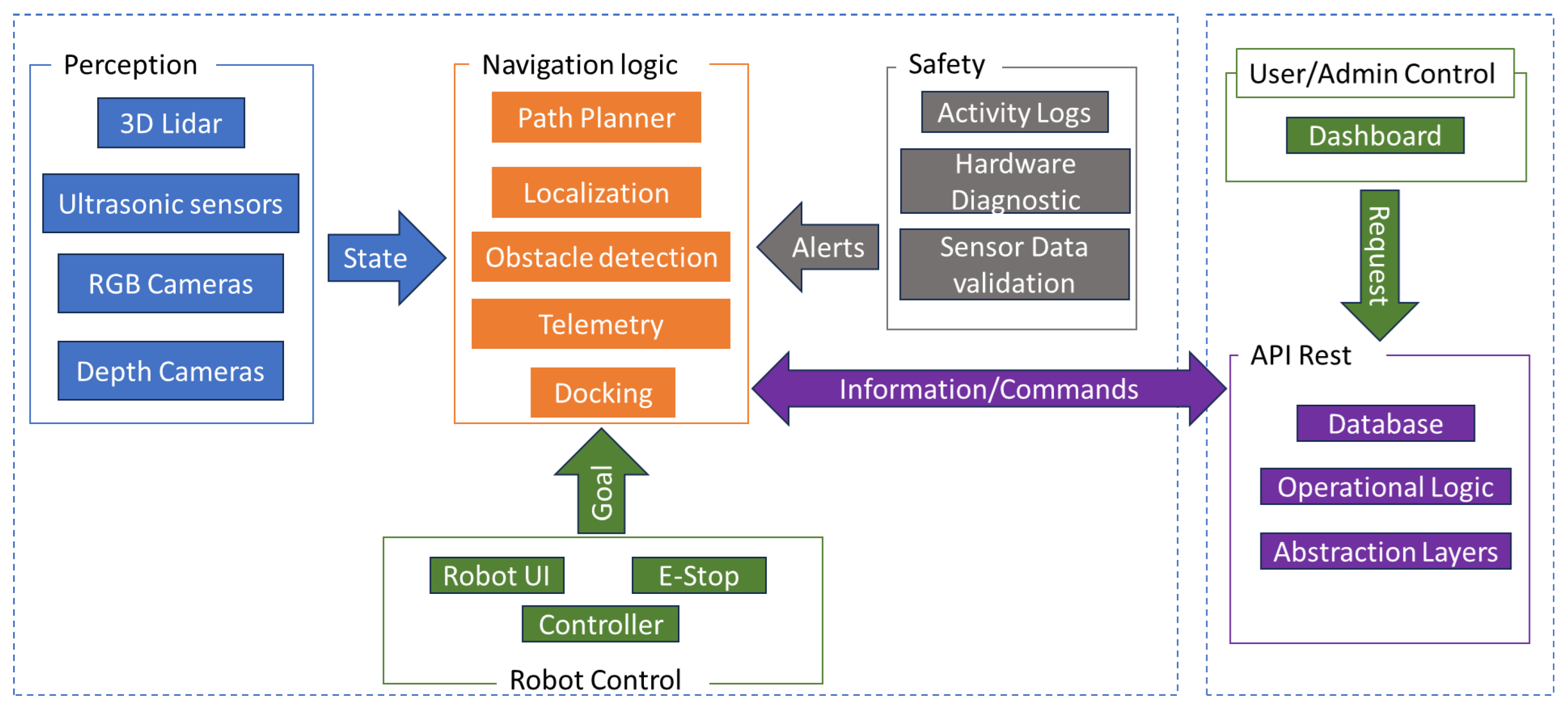
Figure 2 provides an overview of the software architecture that enables autonomy in the Panthera robot. The robot operates on the Robot Operating System (ROS) and features a main navigation system that updates its state using data from perception and computer vision sensors. An integrated alert system monitors software integrity and logs operational data for debugging purposes. The architecture also includes a cloud-based system to support monitoring and control by the operator, along with a remote control pad that allows manual override in case of emergencies.
The navigation system comprises three primary components: localization, a local planner, and a path tracker. A global planner is deliberately omitted to provide greater flexibility during deployment, as the optimal global planning strategy may vary depending on the specific task—for example, cleaning, navigating to a charging station, or road traversal may each require a different planner.
For localization, an Unscented Kalman Filter (UKF)-based pose estimation approach is used. The initial pose estimate is derived from an Inertial Measurement Unit (IMU) integrated with the LiDAR system. This estimate is further refined using multi-threaded Normal Distributions Transform (NDT) scan matching between a global map point cloud and incoming LiDAR scans. For path tracking, a pure pursuit-based controller has been implemented, demonstrating reliable performance across a wide range of operational scenarios.
3. Proposed Framework
3.1. Flow of the Framework
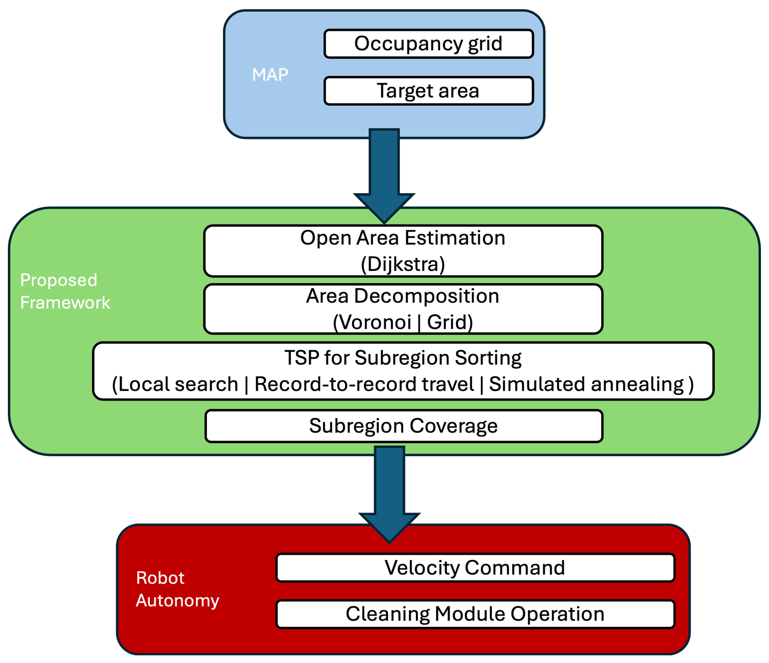
An overview of the proposed framework is presented in
Figure 3. The framework is designed with a focus on non-invasiveness and compatibility with widely adopted navigation techniques employed in ROS-based systems. It utilizes the occupancy grid representation of the environment as the primary input. Given this map and a specified target working area, the framework fist estimates the open area using a Dijsktra-based approach. Then, the framework performs segmentation of the environment into smaller, manageable subregions. In this context, two decomposition strategies, Voronoi-based and grid-based, are analyzed for their effectiveness.
Subsequently, the resulting subregions are optimized and ordered to minimize the overall traversal distance, thereby enhancing operational efficiency. To determine the optimal visiting sequence of subregions, the problem is formulated as a TSP, and multiple optimization heuristics are evaluated, including local search, record-to-record travel, and simulated annealing. Coverage paths for each subregion are generated asynchronously, enabling the robot to commence cleaning tasks while remaining paths are computed concurrently in the background. Furthermore, the framework incorporates integrated control of the robot’s cleaning mechanisms, ensuring seamless and efficient task execution within the defined operational workflow.
3.2. Open Area Estimation
Before initiating the CPP process, the robot must identify accessible and inaccessible regions within the given map, taking into account its physical constraints such as size and maneuverability. In the proposed framework, we employ a Dijkstra-based approach to extract the accessible area of the target map. This method is chosen for two key reasons: first, it systematically explores the graph formed by the open spaces in the map, inherently ignoring regions that are obstructed or unreachable. Second, it is capable of operating in partially known environments, making it robust in dynamic or incomplete mapping scenarios.
In this approach, each open cell is treated as a searchable node. The algorithm evaluates neighboring nodes in order of increasing cost and continues this process until no additional reachable nodes remain. Although Dijkstra’s algorithm is traditionally used to find the shortest path to a specific destination, its application in this framework is adapted to support complete space exploration. Instead of terminating once a goal node is reached, the algorithm continues until all accessible open spaces have been visited, as described in Algorithm 1. If no path exists due to full inaccessibility, the algorithm returns an empty path. Otherwise, it successfully identifies the entire set of reachable nodes, which defines the operational domain for the CPP module. Note that the function “motions” is in charge of making the movements in the exploration process and its four adjacent neighbors, facilitating only movements in the four cardinal directions.
| Algorithm 1 Open Space Exploration |
- 1:
Input: : Map of node IDs to node data : Set of motion primitives - 2:
Output: : Visited nodes with optimal cost - 3:
while is not empty do - 4:
- 5:
- 6:
Remove from - 7:
Add to - 8:
for all motions do - 9:
- 10:
- 11:
- 12:
- 13:
- 14:
if then - 15:
continue - 16:
end if - 17:
if not verify_node(node) then - 18:
continue - 19:
end if - 20:
if then - 21:
Add to - 22:
end if - 23:
end for - 24:
end while - 25:
return
|
3.3. Area Decomposition
To improve the scalability and efficiency of coverage path planning in large environments (environments that surpass the 1000 squared meters), the proposed framework incorporates a decomposition step that partitions the target area into smaller, more manageable subregions. This modular approach offers several advantages. First, it reduces the computational complexity of path planning by localizing the optimization problem within each subregion. Second, it enables parallelization, allowing coverage paths for different subregions to be computed concurrently. Third, it supports asynchronous execution, where the robot can begin cleaning a subregion while paths for the remaining areas are still being generated, thus reducing idle time and improving overall efficiency. Our framework supports two decomposition methods: a Voronoi-based approach and a grid-based approach.
3.3.1. Voronoi-Based Decomposition
Voronoi-based area decomposition is given in Algorithm 2.
Figure 4 shows an example of Voronoi-based decomposition. The process begins by selecting a set of 2D seed points (
). As explained in Algorithm 3, once the free space is estimated, the open area points are shuffled. Then, each seed point is selected at a predefined interval; in our case, a selection of every 15 elements in the open area vector showed a better distribution pattern. For each unique pair of these points, the algorithm calculates the perpendicular bisector necessary for constructing the edges of the Voronoi cells. Then it determines the Voronoi region associated with each seed point (
) by intersecting the corresponding bisectors. If an area is bounded, its intersection points are stored as Voronoi vertices (
); if unbounded, the infinite edges are denoted using a sentinel value. Lastly, the algorithm compiles the ridge information between adjacent regions, detailing both the endpoints (whether finite or at infinity) and the seed points responsible for generating those edges. Voronoi decomposition excels in cluttered environments because its region boundaries naturally conform to obstacle contours, maximizing usable space. Medium-sized robots can leverage Voronoi’s smoother, tighter pathways to navigate efficiently.
| Algorithm 2 Voronoi-Based Decomposition |
- 1:
Input: : Set of 2D seed points - 2:
Output: V : Voronoi vertices, R : Voronoi regions, : Ridge vertex pairs, : Ridge point pairs - 3:
Initialize , , , - 4:
for all distinct pairs do - 5:
Compute the perpendicular bisector between and - 6:
Store bisector as a candidate Voronoi edge - 7:
end for - 8:
for all points do - 9:
Intersect all associated bisectors to form region - 10:
if is bounded then - 11:
Compute region vertices, append to V - 12:
Append list of vertex indices as to R - 13:
else - 14:
Use to mark infinite edges in - 15:
Append to R - 16:
end if - 17:
end for - 18:
for all Voronoi edges between adjacent regions , do - 19:
Identify seed points and ridge vertices - 20:
Append to , and to - 21:
end for - 22:
return
|
| Algorithm 3 Voronoi 2D seed generator |
- 1:
Input: closed_set : List of explored points in real-world coordinates - 2:
Output: voronoid_c : List of grid index tuples marking Voronoi points - 3:
Randomly shuffle the elements of closed_set - 4:
Initialize counter_i - 5:
for all points closed_set do - 6:
Increment counter_i by 1 - 7:
if counter_f − counter_i then - 8:
Reset counter_i - 9:
self.calc_position - 10:
Append to voronoid_c - 11:
end if - 12:
end for - 13:
return voronoid_c
|
3.3.2. Grid-Based Decomposition
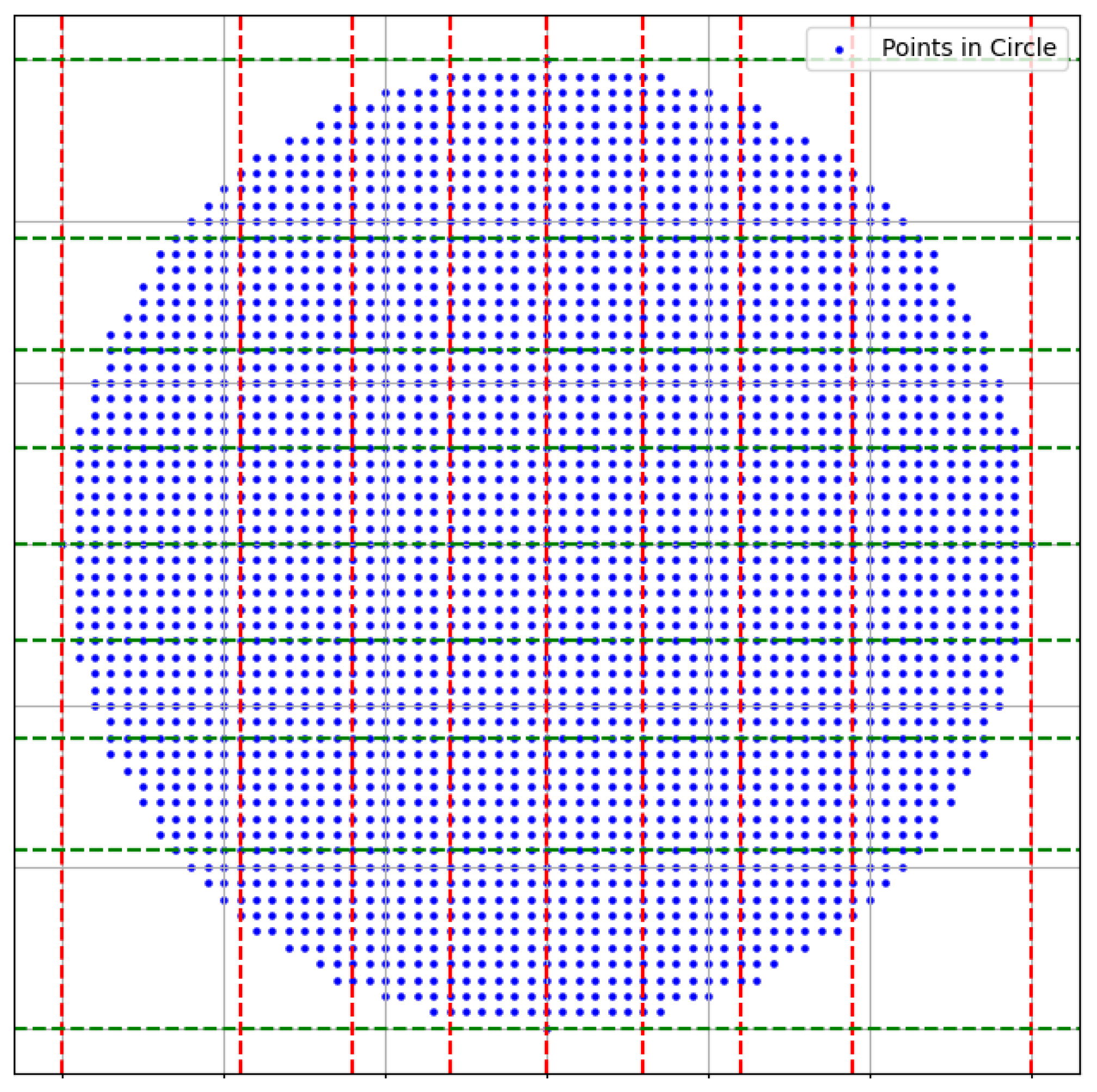
The grid-based decomposition is given in Algorithm 4. The grid splitting method begins by generating a mesh grid of points derived from the open area identified through Dijkstra exploration (interpreted as the Cartesian product of the traversable space). It then organizes the X and Y coordinates and divides them into equally sized segments of a minimum size of four times the robot’s footprint to determine each subregion’s minimum and maximum bounds.
Figure 5 illustrates the identified open areas within a circular map (shown in blue), while red and green dashed lines indicate the vertical and horizontal subdivisions, respectively, offering a clear and structured visualization of the segmented circular domain. The grid approach takes the total free area and fits the grid inside, prioritizing discretization. For large and heavy robots, the grid-splitting algorithm ensures a safe distance from obstacles and prevents unnecessary maneuvers. This approach is particularly beneficial for such robots, as it maintains a uniform distance from obstacles, providing wider safety margins and enabling more predictable, straight-line paths, which reduces the risk of collision and instability during turns.
| Algorithm 4 Grid-Based Decomposition |
- 1:
function make_grid(x, y, n) - 2:
sort(x) - 3:
sort(y) - 4:
split into n equal parts - 5:
split into n equal parts - 6:
Initialize arrays , , , with zeros of length n - 7:
for to do - 8:
ignoring NaNs - 9:
ignoring NaNs - 10:
ignoring NaNs - 11:
ignoring NaNs - 12:
end for - 13:
return , , , - 14:
end function
|
3.4. Determining the Visiting Sequence
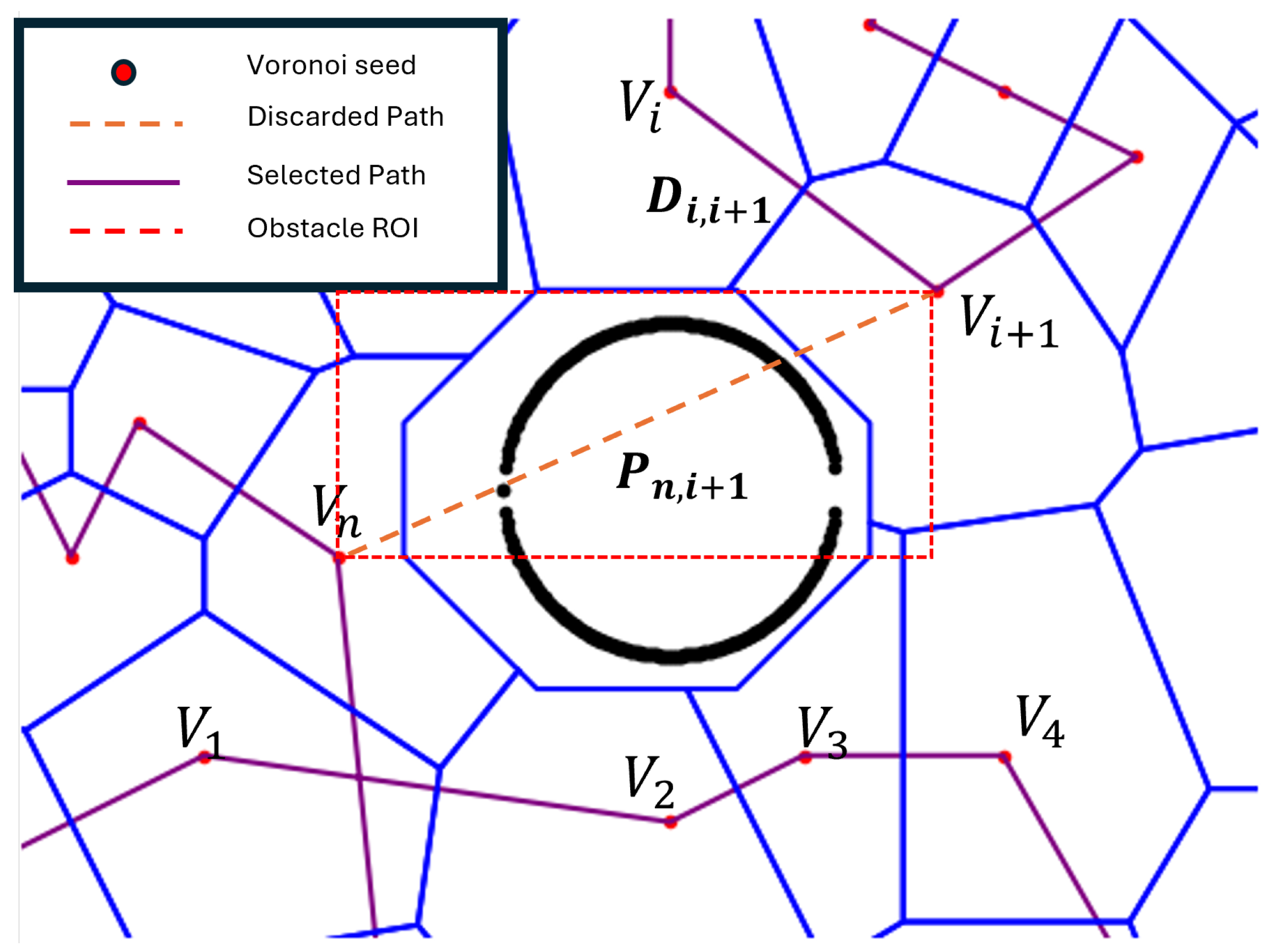
After decomposing into subregions, it is necessary to plan the order in which a robot will go and cover every subregion. The objective is to optimize the energy spent on the course. It is considered that the robot needs to return to the initial location for charging after completion. In this regard, the problem is formulated as a TSP, where each subregion is treated as a node. However, the standard TSP is adapted to be obstacle-aware to increase its effectiveness. This approach has effectively reduced the need to detour around obstacles when determining the optimal traversal paths between subregions.
Figure 6 is used to explain this process considering a Voronoi-based decomposition, where
represents the Voronoi vertices. The Euclidean distance
between the
subregion and the
subregion uses (
1), where
and
denote the coordinates of the exit point of the
subregion and the entry point of the
subregion, respectively.
To discourage paths that intersect obstacles, a penalty term
is introduced. This penalty is given if any obstacle point
lies within the axis-aligned bounding box formed by the two subregion points as explained in (
2).
Let there be
n subregions, and let the ordered list of subregions visited be represented from
. Then, the total path cost
E for the entire route is calculated by (
3)
Given the computational complexity of exact solutions for large instances, we independently analyze three heuristic approaches: local search [
29], record-to-record travel [
30], and simulated annealing [
31]. Local search serves by refining the tour through local modifications. While efficient, its greedy behavior can lead to entrapment in local optima. Record-to-record travel mitigates this by permitting suboptimal solutions within a defined threshold of the best-so-far cost, offering a controlled mechanism to escape local minima. On the other hand, simulated annealing probabilistically accepts higher-cost solutions according to a temperature schedule, enabling broader exploration of the solution space. By evaluating these methods independently, we assess their relative effectiveness in generating high-quality visiting sequences within the constraints of computational efficiency.
3.4.1. Local Search
This algorithm utilizes a local search heuristic approach to compute an approximate solution using a neighborhood-based, iterative improvement strategy. It employs a defined perturbation scheme (the two-opt method chosen in our case study because it delivers real-time results) to generate neighboring solutions, which are slight variations of the current tour. Each neighbor is evaluated to determine whether it yields a lower total travel cost than the existing solution. The current tour is updated upon identifying an improved solution, and the search proceeds from this new point. The procedure adopts a first-improvement approach, terminating the neighborhood exploration when a better solution is encountered. This process continues iteratively until no further improvements can be found (signifying convergence to a local minimum). Even though the algorithm can handle a timeout interval in practice, disabling it to prioritize improvement was feasible, as real-time results were achievable in this case.
Algorithm 5 explains the entire process. Here
D corresponds to the matrix containing the distances from each subregion. The optimal initial tour can be a random path necessary to kickstart the algorithm.
x and
are auxiliary variables to handle each solution in the estimation process and its cost.
| Algorithm 5 Local Search for TSP |
- 1:
D : Distance matrix of size - 2:
: Optional initial tour - 3:
P : Neighborhood generation scheme (default: two_opt) - 4:
T : Maximum time allowed (optional; defaults to unlimited) - 5:
x, : Current solution and its cost from setup_initial_solution(D, ) - 6:
improvement : Boolean flag to check for improvements (initially True) - 7:
stopEarly : Boolean flag to stop if time limit is reached (initially False) - 8:
Start timer - 9:
while improvement and not stopEarly do - 10:
improvement ← False - 11:
for all in neighborhood generated by P do - 12:
if elapsed time then - 13:
stopEarly ← True - 14:
break - 15:
end if - 16:
= compute_permutation_distance(D, ) - 17:
if then - 18:
, - 19:
improvement ← True - 20:
break - 21:
end if - 22:
end for - 23:
end while - 24:
return x,
|
3.4.2. Record-to-Record Travel
Record-to-record travel begins with an initial tour, either randomly generated or user-defined, and iteratively applies small perturbations through random swaps to explore the solution space. In our implementation, each perturbed tour is further refined using the Lin–Kernighan heuristic before evaluation, enhancing the local optimality of candidate solutions. At each iteration, a new candidate tour is accepted if its cost is within a predefined threshold of the best-known (record) tour. This threshold guides the algorithm to explore suboptimal solutions without deviating too far from promising regions of the search space. The process continues for a specified number of iterations, with the best solution found throughout retained as the final output. RRT offers a balance between exploration and exploitation, making it effective for approximating high-quality solutions in complex TSP instances. The flow of record-to-record travel is given in Algorithm 6.
| Algorithm 6 Record-to-Record for TSP |
- Require:
Distance matrix D, initial solution (optional), maximum iterations - Ensure:
Best found solution and its cost - 1:
number of nodes in D - 2:
initial solution (random if not provided) - 3:
cost of x using D - 4:
, - 5:
for to do - 6:
copy of x - 7:
Randomly swap two elements in - 8:
Lin–Kernighan ▹ Apply local improvement - 9:
cost of using D - 10:
if then - 11:
- 12:
- 13:
if then - 14:
- 15:
- 16:
end if - 17:
end if - 18:
end for - 19:
return
|
3.4.3. Simulated Annealing
Simulated annealing is a probabilistic optimization algorithm inspired by the thermal annealing process in metallurgy. As given in Algorithm 7, the method begins with an initial tour and iteratively generates neighboring solutions through small perturbations. Worse solutions may be accepted with a probability governed by a temperature parameter, enabling the algorithm to escape local minima. The temperature gradually decreases according to a predefined cooling schedule, reducing the likelihood of accepting inferior solutions over time. This balance between exploration and exploitation allows SA to effectively approximate near-optimal solutions to the TSP. Here, the distance matrix contains the distances from all cities to sort temperature and cooling rate, which are the two hyperparameters that define the main behavior of algorithm. Temperature defines how much risk the algorithm takes or how many bad or suboptimal routes it will take; on the other hand, the cooling rate is the control at which temperature will decrease.
3.5. Subregion Coverage Planning
Each subregion is processed using a grid-based coverage planning algorithm to generate the final path the robot will follow to perform cleaning. This planning runs in the background while the robot navigates, and the resulting path is translated into a sequence of navigation goals.
The algorithm iterates over all traversable cells within the subregion using the four cardinal directions (north, south, east, west). In practice, using a four-direction approach has shown a decrement in time processing, presenting similar results as an eight-direction boustrophedon. At each step, the current cell is marked as visited. If a cell has already been visited, the algorithm selects an alternative unvisited cell. This process continues until all reachable positions have been covered. The resulting path is output as an ordered list of navigation goals and is formally described in Algorithm 8.
The logic for selecting the initial starting position is detailed in Algorithm 9. It uses the direction vector and initial pose to guide coverage in alignment with the longer side of the subregion, maximizing sweep efficiency.
| Algorithm 7 Simulated Annealing for TSP |
- 1:
cities: List of cities - 2:
n: number of cities - 3:
currentRoute: GenerateInitialRandomRoute (cities) - 4:
distanceMatrix: n × m matrix - 5:
currentDistance: calculateTotalDistance (currentRoute, distanceMatrix) - 6:
bestRoute: currentRoute - 7:
bestDistance: currentDistance - 8:
temperature: initialTemperature - 9:
numberIterations: Any number from 1 to Infinite - 10:
coolingRate: number between 0.0 to 0.99 - 11:
for do - 12:
newRoute = generateNeighbor (currentRoute) - 13:
newDistance = calculateTotalDistance (newRoute, distanceMatrix) - 14:
delta = newDistance - currentDistance - 15:
if OR then - 16:
currentRoute = newRoute - 17:
currentDistance = newDistance - 18:
if then - 19:
bestRoute = currentRoute - 20:
bestDistance = currentDistance - 21:
end if - 22:
end if - 23:
temperature = temperature × coolingRate - 24:
end for - 25:
return bestRoute, bestDistance
|
| Algorithm 8 Grid-Based Coverage Planning for Subregions |
- 1:
grid: The space where the robot will move as a list of cords - 2:
startX, start y: calculateStartPosition (grid) - 3:
directions: matrix of n × n; n is the number of directions in which the robot can move - 4:
nRows: number of rows in the grid - 5:
nCols: number of columns in the grid - 6:
visited: nRows × nCols matrix initialized to False - 7:
finalPath: empty list - 8:
stack: empty stack - 9:
Push (startX, startY) in stack - 10:
visited[startX][startY] = True - 11:
Append (startX, startX) in finalPath - 12:
directions = [(0, 1), (1, 1), (1, 0), (1, −1), (0, −1), (−1, −1), (−1, 0), (−1, 1)] - 13:
while stack is not empty do - 14:
currentRow, currentCol = stack[:−1] - 15:
for Each direction in directions do - 16:
newRow = currentRow + direction[0] - 17:
newCol = currentCol + direction[1] - 18:
if AND AND AND AND NOT visited[newRow][newCol] then - 19:
visited[newRow][newCol] = True - 20:
Append (newRow, newCol) in finalPath - 21:
Push (newRow, newCol) in stack - 22:
end if - 23:
end for - 24:
end while - 25:
return finalPath
|
| Algorithm 9 Find Start Position |
- 1:
Input: , , (lists of x and y coordinates) - 2:
Output: , (sweep direction and start position) - 3:
- 4:
- 5:
- 6:
for
to
do - 7:
- 8:
- 9:
- 10:
if then - 11:
- 12:
- 13:
- 14:
end if - 15:
end for - 16:
return ,
|
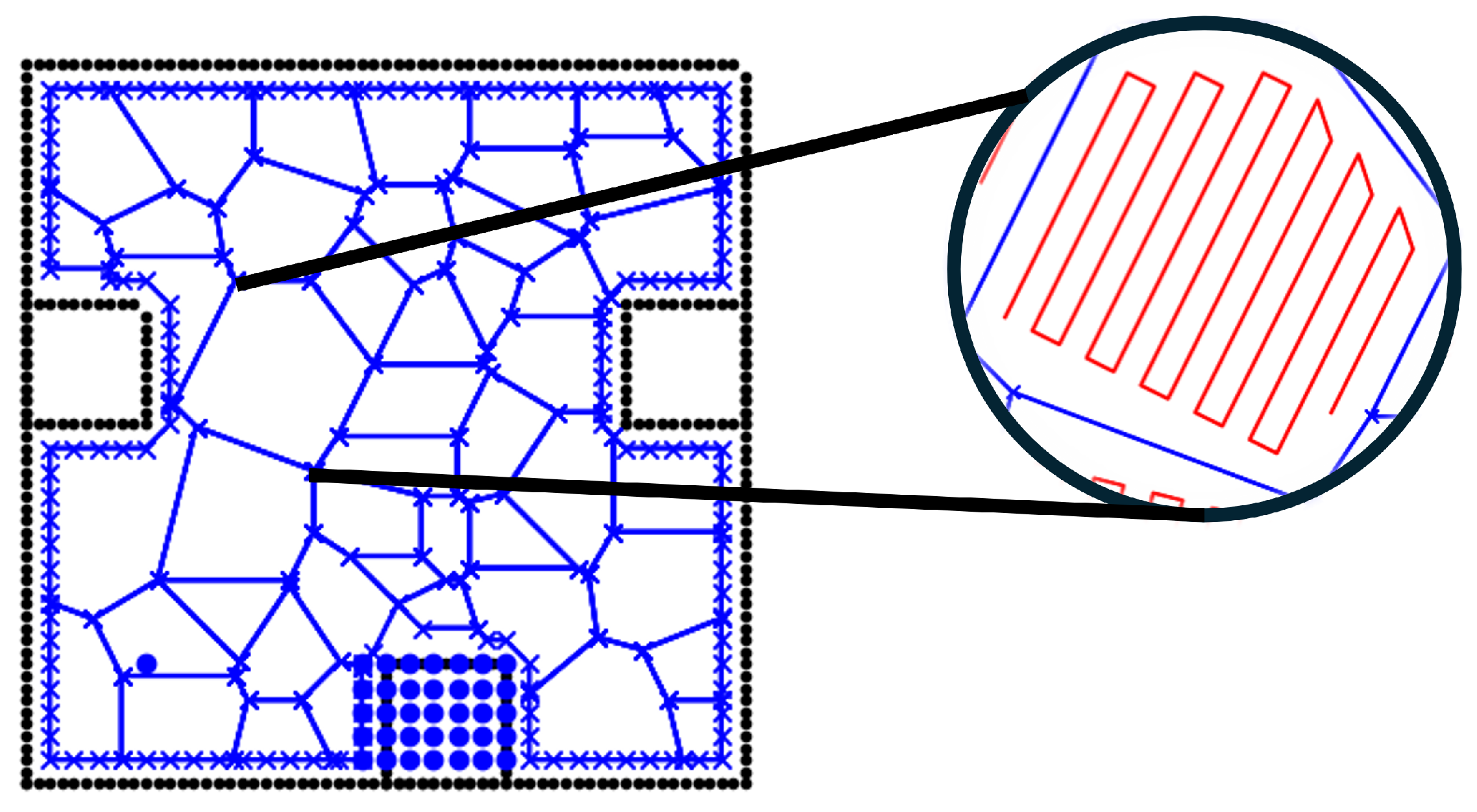
Figure 7 presents a visual example of a coverage path within a subregion obtained through Voronoi decomposition. The blue boundary denotes the Voronoi-defined region to be cleaned, while the red lines illustrate the generated coverage path that the robot follows to complete the task.
4. Results
4.1. Simulations
We conducted Python 3.8.3-based simulations to evaluate all combinations of the proposed framework, resulting in six different configurations: Voronoi with local search, Voronoi with record-to-record travel, Voronoi with simulated annealing, grid-based with local search, grid-based with record-to-record travel, and grid-based with simulated annealing. The simulations were performed on a PC equipped with an Intel Core i7-8550U processor, 16 GB of RAM, and an NVIDIA GeForce MX150 GPU. Please note that GPU is not utilized for path planning.
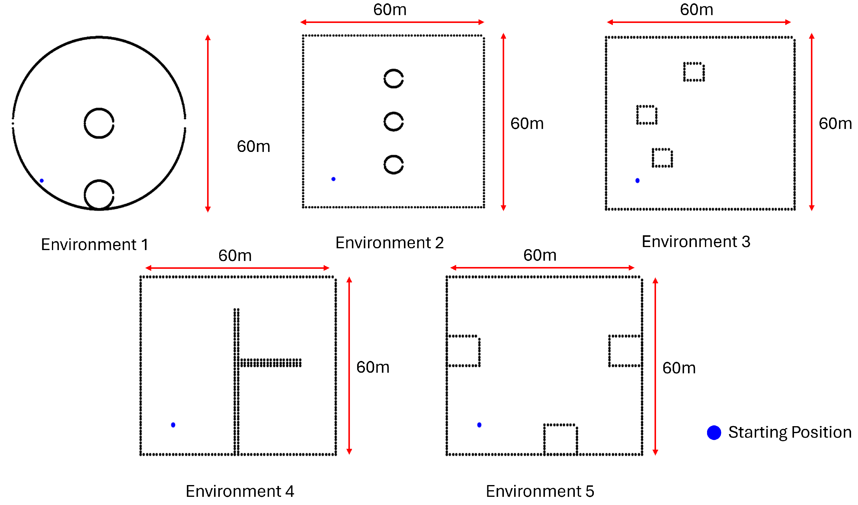
Five different environments with diverse characteristics were selected for the simulations (see
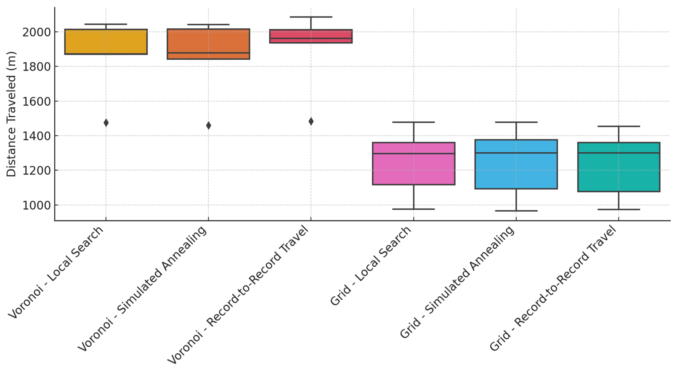
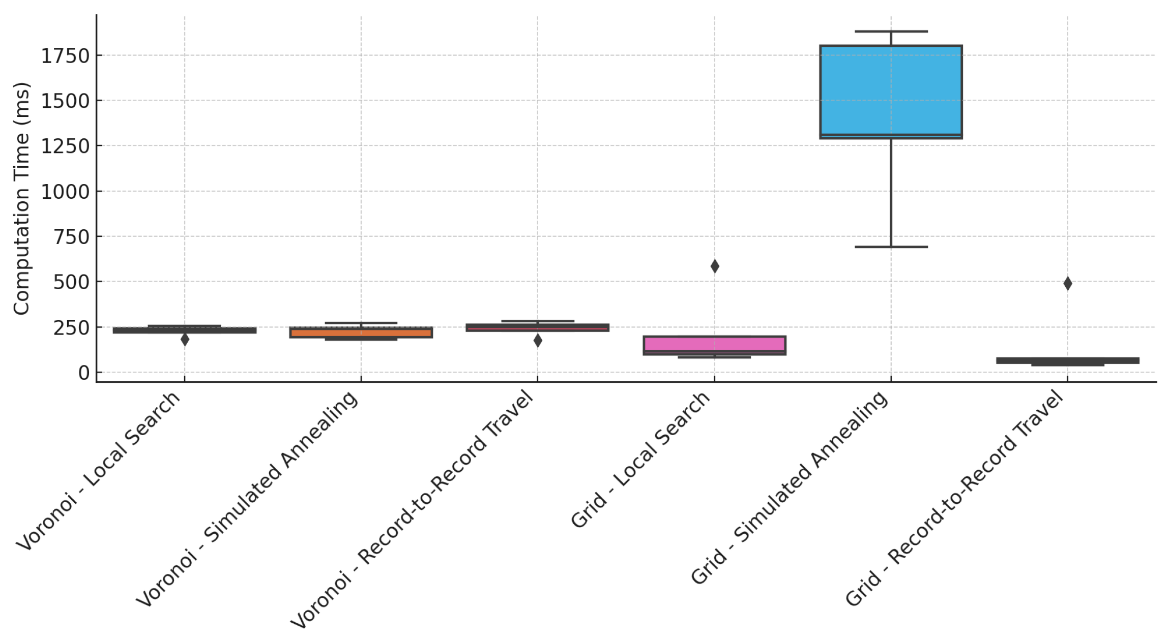
Figure 8). Area coverage, computation time, and path distance were considered the performance metrics. The performance of the CPP variants of the proposed framework is given in
Table 1 and
Table 2,
Figure 9,
Figure 10, and
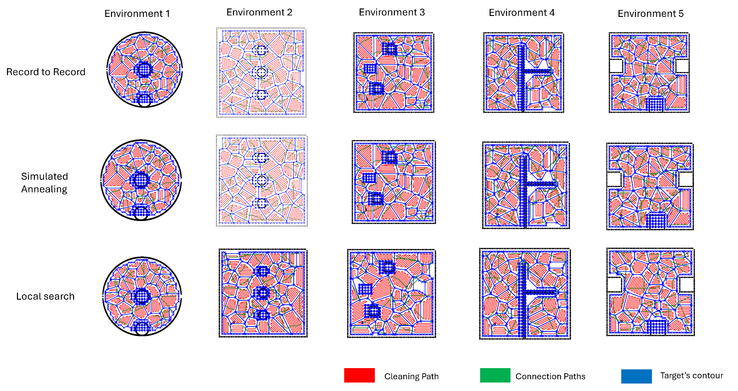
Figure 11, respectively. The coverage paths achieved by Voronoi-based decomposition using local search, record-to-record travel, and simulated annealing for TSP are shown in
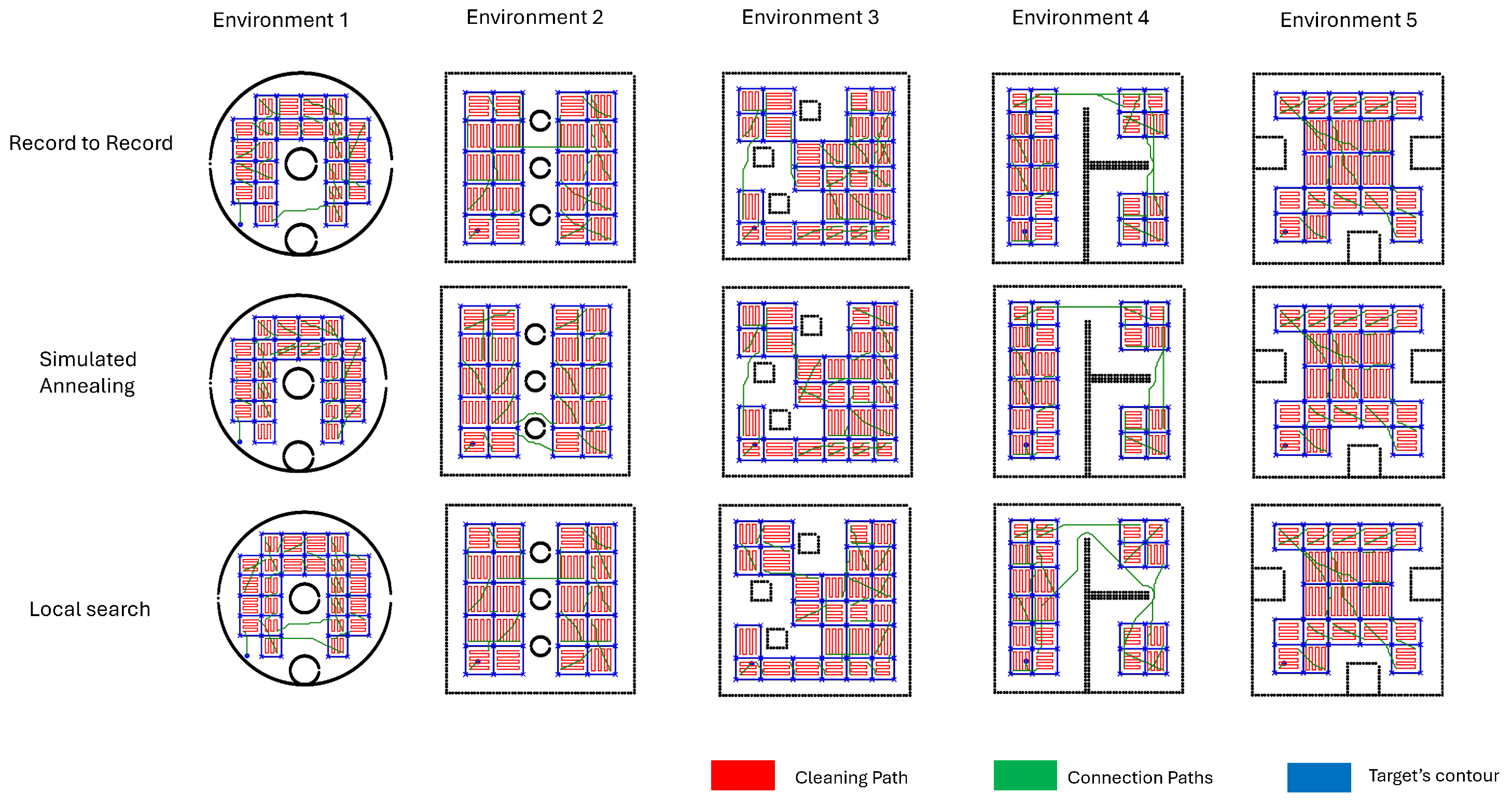
Figure 12. The coverage paths achieved by grid-based decomposition using local search, record-to-record travel, and simulated annealing for TSP are shown in
Figure 13.
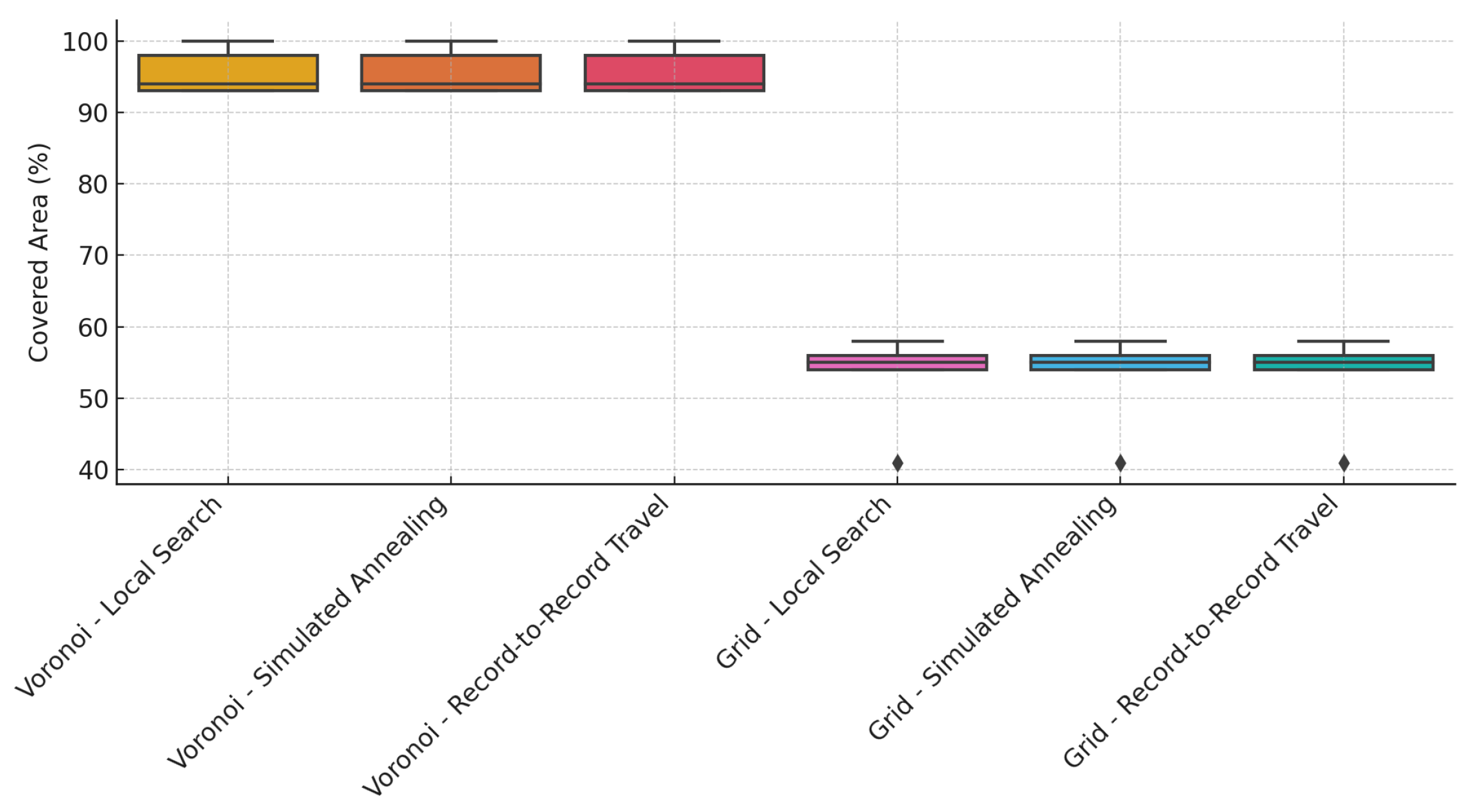
Environment 1 was a circular-shaped area with a diameter of 60 m. The Voronoi-based decomposition resulted in 93% coverage, with identical coverage outcomes across all TSP-solving methods. In contrast, the grid-based decomposition achieved only 56% coverage. Among the Voronoi-based cases, simulated annealing yielded the lowest computational time (194 ms) and the shortest distance traveled by the robot (1460.40 m). Record-to-record travel produced the highest computational time (230 ms) and the longest traveled distance (1483 m), while local search showed intermediate performance in both metrics.
Similar to Environment 1, the CPP using Voronoi decomposition consistently resulted in significantly higher area coverage compared to grid-based decomposition. Moreover, the area coverage was independent of the TSP-solving method in both decomposition approaches. The average area coverage across all environments was 95.6% for Voronoi-based decomposition and 52.8% for grid-based decomposition, indicating the clear superiority of the Voronoi approach. For the Voronoi-based cases, the average computation times for local search, simulated annealing, and record-to-record travel were 225.6 ms, 226.2 ms, and 239.6 ms, respectively. The corresponding average distances traveled by the robot were 1855 m, 1847.5 m, and 1895.3 m. These results suggest that local search is the most computationally efficient method, while simulated annealing yields the shortest travel path. Record-to-record travel performed the worst, with the highest average computation time and path distance. However, the variation between the best and worst performers was only 6% in computation time and 3% in path distance, indicating overall comparable performance among the methods.
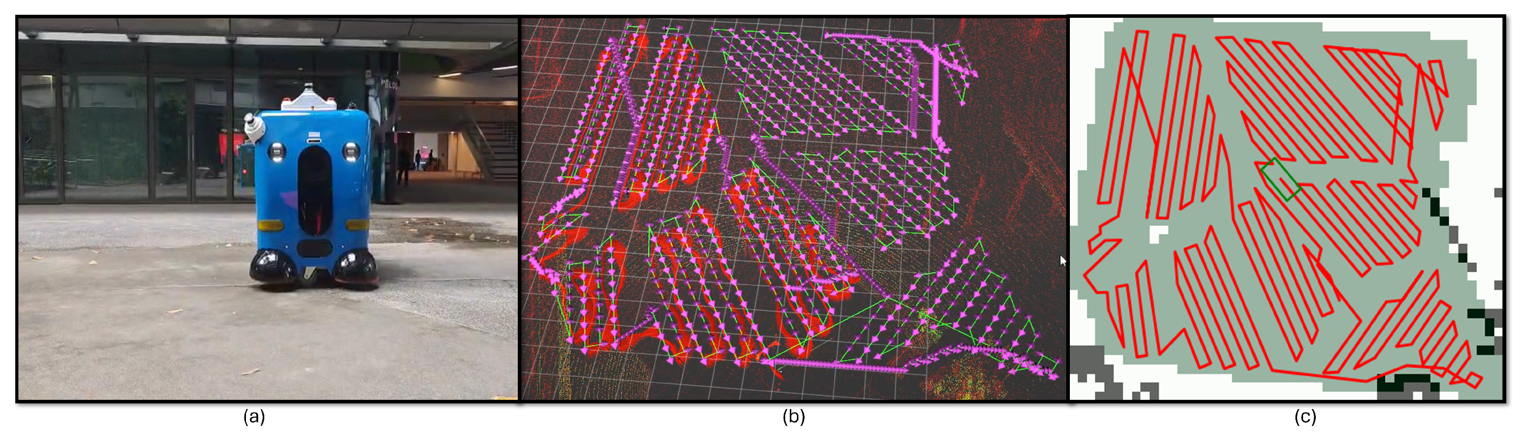
4.2. Robot Hardware Experiments
A hardware test was conducted to validate the real-world applicability of the proposed method. The experiment took place in a 19 m × 17 m environment with cluttered obstacles. Voronoi-based decomposition with local search was used for this case study. The robot during the experiment is shown in
Figure 14a, and the coverage path, visualized through Rviz, is shown in
Figure 14b. The robot was able to achieve 84% area coverage (see
Figure 14c for coverage map) with a total travel distance of 384.85 m, demonstrating the effectiveness of the proposed CPP framework in achieving acceptable performance in real-world scenarios. During the experiments, the robot’s real-world constraints, such as wheel drift and space warping in the map (which causes the localization algorithm to diverge from its actual position), forced the robot to replan its movement in order to align with the path. This issue, in turn, degraded the coverage performance.


