Revisiting the Relationship Between the Scale Factor (a(t)) and Cosmic Time (t) Using Numerical Analysis

Abstract

Background: Current cosmological fits typically assume a direct relation between cosmic time (t) and the scale factor ($a\left(t\right)$), yet this ansatz remains largely untested across diverse observations. Objectives: We (i) test whether a single power-law scaling ($a\left(t\right)\propto t^{\alpha }$) can reproduce late- and early-time cosmological data and (ii) explore whether a dynamically evolving ($\alpha \left(t\right)$), modeled as a scalar–tensor field, naturally induces directional asymmetry in cosmic evolution. Methods: We fit a constant-$\alpha$ model to four independent datasets: 1701 Pantheon+SH0ES supernovae, 162 gamma-ray bursts, 32 cosmic chronometers, and the Planck 2018 TT spectrum (2507 points). The CMB angular spectrum is mapped onto a logarithmic distance-like scale ($\mu ={log}_{10}{D}_{\ell }$), allowing for unified likelihood analysis. Each dataset yields slightly different preferred values for $H_0$ and $\alpha$; therefore, we also perform a global combined fit. For scalar–tensor dynamics, we integrate $\alpha \left(t\right)$ under three potentials—quadratic, cosine, and parity breaking (${\alpha }^{3}sin\alpha$)—and quantify directionality via forward/backward evolution and Lyapunov exponents. Results: (1) The constant-$\alpha$ model achieves good fits across all datasets. In combined analysis, it yields $H_0\simeq 70\mathrm{km}{\mathrm{s}}^{-1}{\mathrm{Mpc}}^{-1}$ and $\alpha \simeq 1.06$, outperforming $\Lambda$CDM globally ($\Delta \mathrm{AIC}\simeq 401254$), though $\Lambda$CDM remains favored for some low-redshift chronometer data. High-redshift GRB and CMB data drive the improved fit. Numerical likelihood evaluations are approximately three times faster than for $\Lambda$CDM. (2) Dynamical $\alpha \left(t\right)$ models exhibit time-directional behavior: under asymmetric potentials, forward evolution displays finite Lyapunov exponents (${\lambda }_L\sim {10}^{-3}$), while backward trajectories remain confined (${\lambda }_L<0$), realizing classical arrow-of-time emergence without entropy or quantum input. Limitations: This study addresses only homogeneous background evolution; perturbations and physical derivations of potentials remain open questions. Conclusions: The time-scaling approach offers a computationally efficient control scenario in cosmological model testing. Scalar–tensor extensions naturally introduce classical time asymmetry that is numerically accessible and observationally testable within current datasets. Code and full data are available.

1. Introduction

Modern cosmology typically assumes that cosmic time (t) can be globally identified with the evolution of the scale factor ($a\left(t\right)$), which increases monotonically in a homogeneous and isotropic universe [1]. However, increasingly detailed observations of large-scale structure suggest that this assumption may be overly simplistic. Recent large-area X-ray and optical surveys have mapped Quipu, the most massive supercluster identified to date [2]. Earlier work by de Vaucouleurs [3] already indicated that galaxies embedded in such dense environments expand more slowly than the global Hubble flow—a phenomenon now called differential expansion. In other words, cosmic expansion is not spatially uniform: it proceeds at a reduced rate in rich cores such as Virgo [4] and at an enhanced rate in low-density outskirts [5].

However, the physical connection between differential expansion and the local passage of time remains unclear. A variety of studies, from technical analyses in quantum gravity [6] to broader conceptual perspectives on time and gravitation [7,8], have examined how gravity might influence temporal rates. Some analyses have derived extreme yet finite time dilations near black holes [9], while others have recast gravitational acceleration as a gradient in the local clock rate [10,11]. Despite this diverse body of work, Balasubramanian [12] and Moore [13] observe that the fundamental nature of time has advanced little since the early twentieth century.

Modern cosmology typically adopts a pragmatic stance: cosmic time is identified with the scale factor ($a\left(t\right)$) or, equivalently, its logarithm. This convention is well motivated in a homogeneous and isotropic universe, where $a\left(t\right)$ increases monotonically [14,15]. However, increasing observational evidence for late-time inhomogeneity raises a question. If expansion can vary spatially, can a single global t remain physically meaningful? Conversely, if a region undergoes net collapse, does that imply a reversal of time?

These considerations prompt a reassessment of what redshift measurements truly encode. Rather than representing purely spatial expansion, observed redshifts may incorporate the cumulative effect of an evolving temporal scale. When gravitational fields modulate local clock rates, space and time become operationally coupled on cosmological scales. Therefore, introducing a time-dependent power-law exponent ($\alpha \left(t\right)$) provides a minimal, testable model capable of explaining late-time acceleration as an emergent consequence of temporal scaling rather than as evidence for an additional dark-energy component.

A concrete illustration comes from the redshift of the cosmic microwave background (CMB). In the power-law model ($a\left(t\right)\propto t^{\alpha }$), the wavelength stretch encodes the cumulative effect of the time-scaling exponent. Photons released at recombination with ${\lambda }_{\mathrm{emit}}\approx 0.9\mathsf{\mu }\mathrm{m}$ (near-infrared) reach us today at ${\lambda }_{\mathrm{obs}}\approx 1\mathrm{mm}$, corresponding to $z\approx 1100$ and matching the CMB intensity peak near 160 GHz. Hence the cosmic redshift can be read as the $a\left(t_0\right)/a\left(t_{\mathrm{emit}}\right)$ ratio or, equivalently, as the accumulated time scaling governed by $\alpha \left(t\right)$. From this perspective the familiar four-dimensional spacetime—in which time is the fourth coordinate and sets the overall scale—can be reformulated as a dynamically evolving “time-scale” geometry in which temporal scaling itself drives cosmological evolution.

Within this perspective, even classical general relativity admits a richer temporal structure once the expansion history is allowed to scale non-trivially. Therefore, we investigate whether a slowly varying exponent in the relation expressed as $a\left(t\right)\propto t^{\alpha \left(t\right)}$ can replicate the key signatures of cosmic acceleration and structure growth without introducing new matter fields beyond a standard scalar–tensor sector.

To this end, we revisit the standard power-law ansatz and confront it with recent Type Ia supernovae (Pantheon+SH0ES) [16,17,18,19,20,21,22], cosmic-chronometer [23], gamma-ray-burst [24], and CMB data [25]. We then extend the model to a scalar–tensor theory, adopting the Brans–Dicke action with a potential, where the $\alpha \left(t\right)$ exponent is promoted to a dynamical field coupled to curvature [26,27].

In this framework, $\alpha \left(t\right)$ plays the role of an effective scalar degree of freedom that modulates the expansion rate, much like the scalar field in the Brans–Dicke or other scalar–tensor models [27]. Treating $\alpha \left(t\right)$ as a slowly varying function keeps the analysis agnostic about the underlying microphysics while capturing potential departures from the standard expansion history and providing a phenomenological link between observational tensions and modified-gravity theories.

We further test whether mild inhomogeneities, when coupled with a variable $\alpha \left(t\right)$, can generate an effective arrow of time while remaining consistent with current data. The goal of this paper is not to invoke new particles but to determine whether adjusting the representation of cosmic time can illuminate persistent tensions such as the Hubble rate discrepancy.

This paper is organized as follows. Section 2 details the numerical scheme and datasets. Section 3 compares model predictions with observations. Section 4 discusses limitations and future extensions. A complete nomenclature of variables and parameters is provided in Appendix A for reference, along with all code and data for reproducibility.

2. Methods

This section recalls standard cosmological relations and shows how they behave when a single exponent ($\alpha$) is allowed to change slowly with cosmic time. No extra physics is introduced; we only adjust the interpretation of familiar equations.

2.1. Friedmann–Lemaître–Robertson–Walker (FLRW) Background

We work in a spatially flat, homogeneous, and isotropic universe described by the Friedmann–Lemaître–Robertson–Walker (FLRW) metric. The Friedmann equations read

$$\begin{array}{cc}\hfill H^2\left(t\right)& ={\left({\displaystyle \frac{\dot{a}}{a}}\right)}^2={\displaystyle \frac{8\pi G}{3}}\rho \left(t\right),\hfill \end{array}$$

(1)

$$\begin{array}{cc}\hfill {\displaystyle \frac{\ddot{a}}{a}}& =-{\displaystyle \frac{4\pi G}{3}}\left[\rho \left(t\right)+{\displaystyle \frac{3p\left(t\right)}{c^2}}\right],\hfill \end{array}$$

(2)

where $H\left(t\right)$ is the Hubble rate, $\rho \left(t\right)$ is the total energy density, and $p\left(t\right)=w\rho \left(t\right)c^2$ is the pressure of a perfect fluid with constant equation-of-state parameter w.

Under this assumption, the scale factor evolves as a power law:

$$a\left(t\right)\propto t^{\alpha },\alpha ={\displaystyle \frac{2}{3(1+w)}}.$$

(3)

Specific values of w recover the standard cosmological eras:

$$w=\frac{1}{3}\Rightarrow \alpha =\frac{1}{2}\left(\mathrm{radiation}\right),w=0\Rightarrow \alpha =\frac{2}{3}\left(\mathrm{matter}\right),w=-1\Rightarrow \alpha \to \infty (\mathrm{de}\mathrm{Sitter}).$$

(4)

2.2. A Slowly Varying Exponent

Standard power-law solutions such as Equation (3) describe individual cosmic eras but switch abruptly between them. To link these regimes more smoothly, we let the exponent depend on cosmic time:

$$a\left(t\right)={\left({\displaystyle \frac{t}{t_0}}\right)}^{\alpha \left(t\right)},$$

(5)

with $t_0$ fixed to the present epoch. Differentiating gives

$$H\left(t\right)={\displaystyle \frac{\dot{a}}{a}}={\displaystyle \frac{\alpha \left(t\right)}{t}}+\dot{\alpha }\left(t\right)ln\left({\displaystyle \frac{t}{t_0}}\right).$$

(6)

The second term is small when $\alpha \left(t\right)$ varies slowly and is typically negligible in observational analyses (such as those using Type Ia supernovae), where $\alpha \left(t\right)$ is effectively constant at the present time.

2.3. Regional Expansion

Observations hint that the expansion rate may differ across large-scale structures such as the Quipu supercluster. In a simple phenomenological form, one may write

$$H(t,\mathbf{x})\simeq {\displaystyle \frac{\alpha (t,\mathbf{x})}{t}},$$

(7)

acknowledging that exact homogeneity is an idealization. The present work concentrates on the global average ($\alpha \left(t\right)$); spatial dependence is set aside for future study.

2.4. Acceleration Criterion in Terms of $\alpha$

Cosmic acceleration is determined by the sign of the second time derivative of the scale factor. From Equation (5), assuming a slowly varying exponent ($\alpha \left(t\right)\approx \mathrm{const}$), we find

$${\displaystyle \frac{\ddot{a}}{a}}={\displaystyle \frac{\alpha (\alpha -1)}{t^2}}.$$

(8)

This expression shows that

• $\alpha <1$ implies $\ddot{a}<0$—the universe is decelerating;
• $\alpha =1$ implies $\ddot{a}=0$—constant-rate expansion;
• $\alpha >1$ implies $\ddot{a}>0$—the universe is accelerating.

Therefore, the condition of $\alpha >1$ provides a simple and direct criterion for accelerated cosmic expansion in this framework. This links the expansion history to a single effective parameter, offering a minimal alternative to introducing a cosmological constant ($\Lambda$).

Note that this acceleration emerges naturally from the power-law ansatz without invoking new energy components. When observational fits yield $\alpha >1$, they are consistent with an accelerating universe—as is currently observed.

2.5. Model Suite

We compare two background expansions. The first serves as a benchmark; the second asks whether a single power-law exponent can model the data without invoking dark energy.

• $\Lambda$CDM.

$$H^2\left(z\right)=H_0^2\left[{\mathrm{\Omega }}_m{(1+z)}^3+{\mathrm{\Omega }}_{\Lambda }\right],{\mathrm{\Omega }}_m+{\mathrm{\Omega }}_{\Lambda }=1.$$

(9)

• Time-scaling.

$$H\left(z\right)=H_0{(1+z)}^{1/\alpha },$$

(10)

which follows from the scale factor of $a\left(t\right)=t^{\alpha }$ with $t_0=1$. Since redshift is defined as $1+z=1/a\left(t\right)=t^{-\alpha }$, it follows that $log(1+z)=-\alpha logt$ or, equivalently, $t={(1+z)}^{-1/\alpha }$. Substituting into $H\left(t\right)=\alpha /t$ gives the observational form of $H\left(z\right)=H_0{(1+z)}^{1/\alpha }$.

We assume spatial flatness (${\mathrm{\Omega }}_k=0$) throughout.

2.6. Datasets

Constraints come from four complementary sources:

• Type Ia supernovae:
  The Pantheon+SH0ES compilation of 1701 supernovae, with full covariance matrix treatment [16,17,18,19,20,21,22].
• Gamma-ray bursts: A calibrated set of 162 long GRBs reaching redshifts up to $z\sim 8$ using empirical Amati relations [24].
• Cosmic chronometers: Thirty-two differential-age measurements of $H\left(z\right)$ obtained from galaxy evolution data [23].
• CMB angular power spectrum: The Planck 2018 temperature–temperature (TT) spectrum, comprising 2507 multipole points [25].

Together, these span the redshift range of $0\lesssim z\lesssim 1100$, probing both the differential expansion rate and integrated-light distance measures.

2.7. CMB Angular Scale Transformation

The Planck 2018 TT power spectrum provides temperature anisotropy amplitudes as a function of the angular multipole (ℓ). To compare these with expansion-based observables in redshift space, we define an approximate mapping of

$$z_{\mathrm{eff}}(\ell )=\kappa ·\ell ,\mathrm{with}\kappa =4.95$$

(11)

so that the first acoustic peak at $\ell \approx 220$ corresponds to the last-scattering redshift $z\approx 1089$. This linear mapping introduces less than 1.5% relative distortion over the range of $\ell \in [30,2500]$, as validated against the redshift distribution of the CMB visibility function (see Appendix A for details).

We then define a pseudo-distance modulus for each multipole as

$${\mu }_{\mathrm{CMB}}(\ell )={log}_{10}\left[{\displaystyle \frac{C_{\ell }}{{\ell }^2}}\right],$$

(12)

where $C_{\ell }$ is the angular power at multipole ℓ. This transformation preserves monotonicity and scale separation, producing a smoothly decreasing curve in $\mu$ space that can be directly compared with SN, GRB, and cosmic-chronometer data.

Uncertainties are propagated via

$${\sigma }_{\mu }=min\left(0.434·{\displaystyle \frac{{\sigma }_{D_{\ell }}}{D_{\ell }}},0.1·{\mu }_{\mathrm{CMB}}\right),$$

(13)

to prevent numerical instabilities at high ℓ values. After this transformation, the CMB data are treated identically to other probes in the log-distance domain, enabling analytic and computationally efficient evaluation of the joint likelihood.

2.8. Distance and Likelihood

Given any cosmological background, the luminosity distance is computed as

$$D_L\left(z\right)=(1+z){\int }_0^z{\displaystyle \frac{c\mathrm{d}{z}^{\prime }}{H\left(z^{\prime }\right)}},$$

(14)

which defines the theoretical distance modulus:

$$\mu \left(z\right)=5{log}_{10}\left[{\displaystyle \frac{D_L\left(z\right)}{\mathrm{Mpc}}}\right]+25.$$

(15)

The constant term of 25 corresponds to the conventional Type Ia supernova calibration, though each dataset requires its own specific zero-point adjustment. Model parameters are obtained by minimizing the ${\chi }^2$ statistic, i.e.,

$${\chi }^2={({\mathit{\mu }}_{\mathrm{obs}}-{\mathit{\mu }}_{\mathrm{th}})}^{\top }{\mathbf{C}}^{-1}({\mathit{\mu }}_{\mathrm{obs}}-{\mathit{\mu }}_{\mathrm{th}}),$$

(16)

and ranked using both the Akaike (AIC) and Bayesian (BIC) Information Criteria [28]. Full routines and datasets are available in the repository.

2.9. Scalar–Tensor Gravity Framework

In scalar–tensor theories, it is common to describe deviations from strict power-law expansion by promoting the parameters governing the expansion rate to dynamical fields. Since $\alpha \left(t\right)$ controls the time scaling of the scale factor, allowing it to evolve dynamically represents a straightforward extension consistent with well-studied scalar–tensor models. This approach introduces no new degrees of freedom beyond those already familiar in classical extensions of general relativity.

This step serves two complementary purposes. First, observational fits suggest that a single constant exponent ($\alpha$) can approximate the late-time expansion history reasonably well, but departures at both low and high redshifts hint at potential time variability. Allowing $\alpha \left(t\right)$ to evolve dynamically provides a natural way to capture possible deviations from strict power-law scaling while remaining within a controlled theoretical framework.

Second, treating $\alpha \left(t\right)$ as a dynamical degree of freedom allows us to investigate whether classical scalar field dynamics can introduce intrinsic temporal asymmetry. In standard cosmology, the arrow of time is typically associated with thermodynamic irreversibility or quantum decoherence. Here, by embedding $\alpha \left(t\right)$ in a scalar–tensor action with explicit curvature coupling, we explore whether directional evolution can emerge purely from classical gravitational dynamics. This formulation allows us to quantify time asymmetry via forward/backward integration and Lyapunov exponents, providing a self-contained mechanism for emergent time directionality within classical general relativity extended by scalar–tensor couplings.

2.9.1. Action and Coupling

Having introduced $\alpha \left(t\right)$ as a dynamical quantity, we require a covariant framework that consistently couples this evolving exponent with gravity. Since $\alpha \left(t\right)$ governs the scaling between space and time, the minimal extension is to introduce it as a scalar field coupled with curvature, following the standard scalar–tensor approach. Specifically, we adopt a Brans–Dicke-type action in which $\alpha$ enters through both a non-minimal coupling with the Ricci scalar and a self-interaction potential. This construction is sufficiently general to recover standard Brans–Dicke theory in appropriate limits while allowing for additional scalar dynamics via $V\left(\alpha \right)$.

The resulting action takes the form of

$$S=\int d^{4}x\sqrt{-g}\left[{\displaystyle \frac{1}{2{\kappa }^2}}R+{\displaystyle \frac{1}{2}}\xi {\alpha }^{2}R-{\displaystyle \frac{1}{2}}{g}^{\mu \nu }{\nabla }_{\mu }\alpha {\nabla }_{\nu }\alpha -V\left(\alpha \right)+{\mathcal{L}}_{\mathrm{m}}\right],{\kappa }^2\equiv 8\pi G.$$

(17)

Here, $\xi$ is a dimensionless non-minimal coupling; taking $\alpha \to 0$ recovers standard general relativity.

Priors

Solar system time-delay measurements from Cassini require $\left|\xi \right|\lesssim 1.2\times {10}^{-5}$ at 95 % C.L. [29], while a Planck PR4 + BAO analysis gives $\left|\xi \right|\lesssim 3\times {10}^{-4}$ [26]. Therefore, throughout, we adopt $\left|\xi \right|\le 3\times {10}^{-4}$, comfortably satisfying current bounds.

Relation to Vanilla Brans–Dicke

Setting $V\left(\alpha \right)=0$ and defining $\phi \equiv \xi {\alpha }^2$, Equation (17) reduces to the canonical Brans–Dicke action:

$$S_{\mathrm{BD}}={\displaystyle \frac{1}{2{\kappa }^2}}\int d^{4}x\sqrt{-g}\left[\phi R-{\displaystyle \frac{{\omega }_{\mathrm{BD}}}{\phi }}{g}^{\mu \nu }{\nabla }_{\mu }\phi {\nabla }_{\nu }\phi +2{\kappa }^2{\mathcal{L}}_{\mathrm{m}}\right],$$

(18)

with

$${\omega }_{\mathrm{BD}}={\displaystyle \frac{1-6\xi }{4\xi }}.$$

(19)

The observational upper limit ($\left|\xi \right|\le 3\times {10}^{-4}$) implies $|{\omega }_{\mathrm{BD}}|\gtrsim \mathcal{O}\left({10}^3\right)$, satisfying the Cassini bound ${\omega }_{\mathrm{BD}}>4\times {10}^4$ once $V\left(\alpha \right)\ne 0$ is included.

Therefore, this framework reproduces Brans–Dicke in the $\xi \ll 1$ limit but departs from it through the presence of a non-trivial potential ($V\left(\alpha \right)$) and by treating $\alpha$ (rather than $\phi$) as the primary field, emphasizing its role as a dynamical e-folding rate.

Connection with the E-Folding Variable

Expressing the scale factor as $a\left(t\right)=exp\left[{\int }^{t}d{t}^{\prime }\alpha \left(t^{\prime }\right)/t^{\prime }\right]$ shows that $\alpha$ generalizes the constant power-law index (n) of $a\propto t^n$. This point of view traces back to Ellis [30] and has been exploited in inflationary reconstruction [1]; the novelty here lies in embedding it consistently in a scalar–tensor action and fitting it to modern data.

Potential Choice and Time Asymmetry

We allow $V\left(\alpha \right)$ to contain odd powers, e.g., $V={\lambda }_2{\alpha }^2+{\lambda }_3{\alpha }^3+\dots$, which break the $\alpha \to -\alpha$ symmetry and induce a small background time asymmetry. Section 3.4 quantifies the effect via Lyapunov exponents and shows that it remains consistent with observations while providing a clear phenomenological discriminator.

Global vs. Local Dynamics

In this work, $\alpha \left(t\right)$ is treated as a spatially homogeneous function describing the cosmic mean expansion rate. Spatial fluctuations ($\delta \alpha (t,\mathbf{x})$) contribute to the metric perturbations in the second order and are analyzed elsewhere. This assumption is justified a posteriori, since the amplitude of $\delta \alpha$ inferred from large-scale structures remains subdominant to the scalar metric potentials.

2.9.2. Field Equations

Varying the action gives

$$\begin{array}{cc}\hfill \square \alpha +\xi R\alpha -{\displaystyle \frac{dV}{d\alpha }}& =0,\hfill \end{array}$$

(20)

$$\begin{array}{cc}\hfill G_{\mu \nu }+{\kappa }^2\xi \left({\alpha }^2{G}_{\mu \nu }-{\nabla }_{\mu }{\nabla }_{\nu }{\alpha }^2+g_{\mu \nu }\square {\alpha }^2\right)& ={\kappa }^2\left(T_{\mu \nu }^{\left(\alpha \right)}+T_{\mu \nu }^{\mathrm{m}}\right).\hfill \end{array}$$

(21)

Here, $\square \equiv {\nabla }^{\mu }{\nabla }_{\mu }$ denotes the covariant d’Alembertian operator acting on scalar fields.

In a flat FLRW background with $\alpha =\alpha \left(t\right)$ and $R\simeq 12H^2$, Equation (20) reduces to

$$\ddot{\alpha }+3H\dot{\alpha }+\xi R\alpha +{\displaystyle \frac{dV}{d\alpha }}=0.$$

(22)

2.9.3. Scalar Potentials

In scalar–tensor cosmologies, the scalar field potential ($V\left(\alpha \right)$) governs both the expansion history and the field’s stability and attractor behavior. We adopt three representative forms to qualitatively explore distinct dynamical regimes, motivated by both phenomenology and higher dimensional geometry.

The quadratic potential, i.e.,

$$V_1\left(\alpha \right)=\frac{1}{2}{m}^2{\alpha }^2,$$

(23)

is widely used in inflationary and quintessence models due to its simplicity and well-understood slow-roll dynamics [27,31].

The cosine potential, i.e.,

$$V_2\left(\alpha \right)=V_{0}cos\alpha ,$$

(24)

is characteristic of axion-like fields and pseudo-Nambu–Goldstone bosons, as it encodes periodic modulations and admits multiple attractor branches [32,33]. Such potentials frequently emerge in models with compactified extra dimensions, where moduli fields inherit periodic structures due to underlying higher dimensional symmetries.

The asymmetric, parity-breaking potential, i.e.,

$$V_3\left(\alpha \right)={\alpha }^{3}sin\alpha ,$$

(25)

explicitly breaks the symmetry under $\alpha \to -\alpha$, enabling solutions that differ under time reversal ($t\to -t$) and thereby supporting an emergent “arrow of time” [34,35,36]. Its structure is heuristically motivated by volumetric scaling in three dimensions (via the cubic prefactor), combined with oscillatory modulations arising from curvature or compactified angular modes (encoded in the sinusoidal term). While not derived from a specific UV-complete theory, this form captures the interplay of nonlinear feedback and geometric asymmetry and serves as a minimal toy model for directionally biased dynamics in scalar–curvature interactions.

Interestingly, scalar fields like $\alpha$ often emerge in extra-dimensional frameworks such as Kaluza–Klein theories, where dimensional reduction yields scalar moduli that couple directly with the four-dimensional Ricci scalar ($R_4$). In this context, $\alpha$ may encode the scale or shape of compactified internal spaces, linking the time dependence of the Hubble flow to dynamical geometry. Moreover, scale-invariant (Weyl-invariant) gravity theories feature a dilaton field that similarly sets mass scales via spontaneous symmetry breaking. The non-minimal coupling (${\alpha }^{2}R$) used in action (17) is the only dimension-4 operator consistent with Weyl symmetry—further supporting the interpretation of $\alpha$ as a geometric scale factor governing both spatial expansion and temporal flow.

2.9.4. Numerical Evolution

The scalar exponent ($\alpha \left(t\right)$) controls the background via the scaling law ($a\left(t\right)\propto t^{\alpha \left(t\right)}$), while the non-minimal coupling term ($\xi {\alpha }^{2}R$) feeds its dynamics back into the geometry. These ingredients allow us to ask whether a time-dependent exponent can account for late-time observables without requiring an explicit dark component and—if the potential is asymmetric—whether it can support an emergent classical arrow of time within the scalar field dynamics.

We evolve the scalar field using the second-order ODE given in Equation (22), with $H\left(t\right)\approx \alpha \left(t\right)/t$ and $R\left(t\right)\approx 12H^2$. We test three potentials: quadratic, cosine, and an asymmetric form $V\left(\alpha \right)={\alpha }^{3}sin\left(\alpha \right)$. Forward and backward integration is performed in time using a fourth-order adaptive Runge–Kutta scheme (solve_ivp) with tolerances of rtol  $={10}^{-8}$ and atol  $={10}^{-10}$.

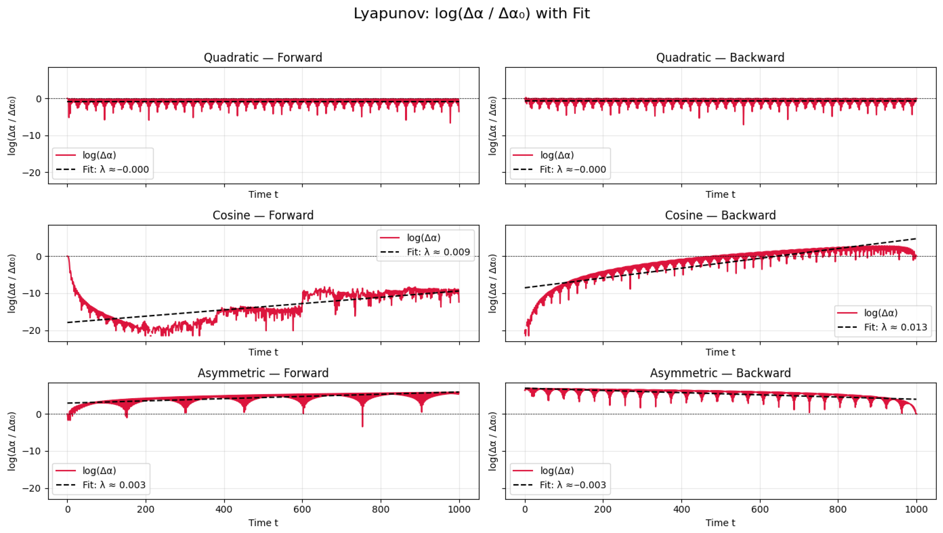
2.9.5. Lyapunov Exponent Computation

To quantify sensitivity to initial conditions and assess time asymmetry, we compute the largest finite-time Lyapunov exponent (${\lambda }_L$). Alongside the reference trajectory $\alpha \left(t\right)$, we evolve a nearby (perturbed) solution (${\alpha }^{\prime }\left(t\right)$) (not a derivative but an independent trajectory with slightly shifted initial conditions) with an initial offset of $\delta {\alpha }_0={10}^{-6}$.

The divergence is measured as

$${\lambda }_L\left(t\right)={\displaystyle \frac{1}{t}}log\left({\displaystyle \frac{|\alpha \left(t\right)-{\alpha }^{\prime }\left(t\right)|}{\delta {\alpha }_0}}\right)$$

(26)

and fitted with a linear trend in $log(\Delta \alpha /\delta {\alpha }_0)$ to extract ${\lambda }_L$. Forward and backward directions are analyzed independently to identify any directional bias or emergent irreversibility.

Three diagnostics are reported: the absolute time-reversal asymmetry, i.e.,

$$\mathcal{A}=\int |{\dot{\alpha }}_{\mathrm{f}}\left(t\right)-{\dot{\alpha }}_{\mathrm{b}}\left(t\right)|dt;$$

(27)

the directional bias, i.e.,

$$\mathcal{B}=\langle {\alpha }_{\mathrm{f}}\left(t\right)-{\alpha }_{\mathrm{b}}\left(t\right)\rangle ;$$

(28)

and the largest Lyapunov exponent (${\lambda }_L$). As presented in the Section 3, although all three models evolve under covariant equations, their temporal behavior differs substantially.

2.10. Computational Pipeline

All calculations were run in Python 3.12. The key libraries are NumPy 2.0.2 [37], SciPy 1.13.1 [38], Pandas 2.2.2 [39], Matplotlib 3.9.2 [40], and emcee 3.1.6 [41]. Parameter estimation first uses differential evolution, then (optionally) an affine-invariant MCMC for posterior sampling. Code is available in Appendix A.

3. Results

Four independent datasets were fitted with the two background models defined in Section 2.5. The analysis proceeds as follows:

• Load observational datasets: Type Ia supernovae, gamma-ray bursts, cosmic chronometers, and CMB constraints.
• Define unified chi-squared functions for both $\Lambda$CDM and time-scaling models, incorporating all four datasets.
• Perform simultaneous parameter estimation using differential evolution global optimization.
• Compute model selection statistics (AIC, BIC, and ${\chi }_{\mathrm{red}}^2$) to assess relative model performance.

This gradual approach ensures a consistent treatment of nuisance parameters (e.g., $M_B$) across datasets while jointly constraining cosmological parameters using multiple independent observational probes.

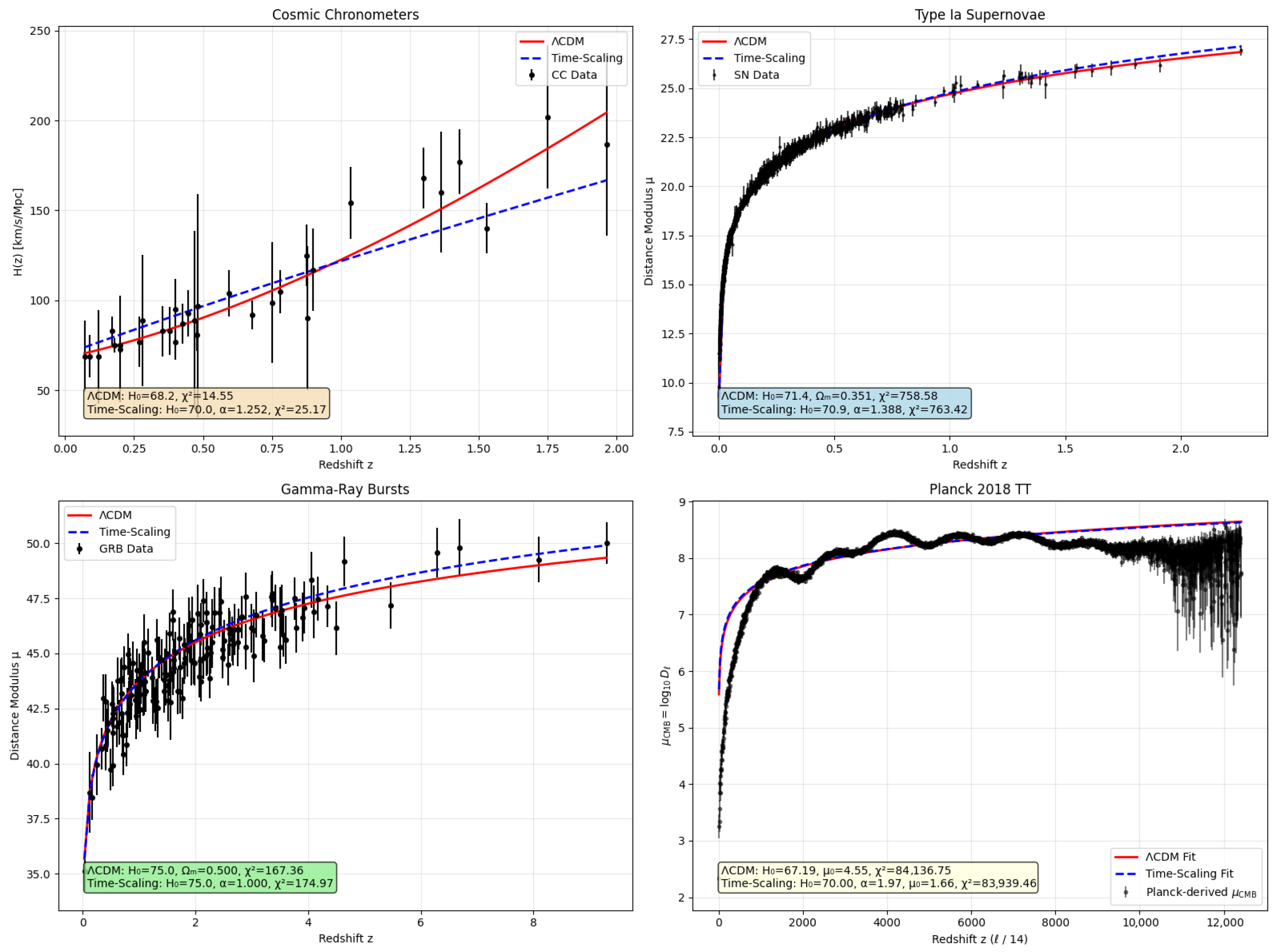
The aim is to test whether a single time-scaling exponent can reproduce late- and early-time observables that are usually attributed to dark energy. Figure 1 and

Table 1. Best-fit parameters and information criteria for each observational sample. Lower AIC and BIC values indicate the preferred description. The time-scaling model shows significantly better performance in the combined analysis, with $\Delta$AIC = 401,254.37.

Data Set (N)	Model	Parameters *	${\mathit{\chi }}^2$	AIC/BIC
CC (32)	$\Lambda$CDM	$H_0=68.16,{\mathrm{\Omega }}_m=0.319$	14.55	18.55/21.49
	Time–Scaling	$H_0=70.00,\alpha =1.252$	25.17	29.17/32.11
SN (1701)	$\Lambda$CDM	$H_0=71.42,{\mathrm{\Omega }}_m=0.351$	758.58	762.58/773.46
	Time–Scaling	$H_0=70.89,\alpha =1.388$	763.42	767.42/778.30
GRB (162)	$\Lambda$CDM	$H_0=75.00,{\mathrm{\Omega }}_m=0.500$	167.36	171.36/177.53
	Time–Scaling	$H_0=75.00,\alpha =1.000$	174.97	178.97/185.15
CMB (2507)	$\Lambda$CDM	$H_0=67.19$	84,136.75	84,138.75/84,144.57
	Time–Scaling	$H_0=70.00,\alpha =1.966$	83,939.46	83,943.46/83,955.09
Combined (4402)	$\Lambda$CDM	$H_0=65.00,{\mathrm{\Omega }}_m=0.357$	626,542.74	626,550.74/626,576.27
	Time–Scaling	$H_0=70.00,\alpha =1.060$	225,288.37	225,296.37/225,321.90

(*) $H_0$ in km s⁻¹ Mpc⁻¹.

summarize the best-fit curves and numerical metrics, while Figure 2 shows the corresponding posterior samples.

3.1. Best Fit to Observational Data

3.1.1. Visual Inspection

In the supernova panel, the red and blue curves are nearly indistinguishable across $0<z\lesssim 2.3$. For gamma-ray bursts, the blue dashed curve (time scaling) sits slightly above the red curve at high redshifts and better follows the upper envelope of the points. In the chronometer panel, the red curve rises more steeply and passes closer to most high z data, whereas the blue curve traces the lower envelope. The CMB panel shows that both models follow the acoustic “wave” pattern after ${\mu }_{\mathrm{CMB}}$ transformation; the time- scaling model does so with a higher $H_0$ and a single exponent ($\alpha$).

3.1.2. Information Criteria

Table 1 lists the best-fit parameters, together with the ${\chi }^2$, AIC, and BIC, for all four samples. Supernovae and chronometers favor $\Lambda$CDM, gamma-ray bursts favor the time-scaling model, and the transformed CMB spectrum shows a mild preference for time scaling, despite its extra parameter. The numerical differences are modest, indicating that a single power-law exponent can compete with a cosmological constant once the data reach $z\gtrsim 4$ and can even accommodate the CMB acoustic structure without altering the sound horizon scale.

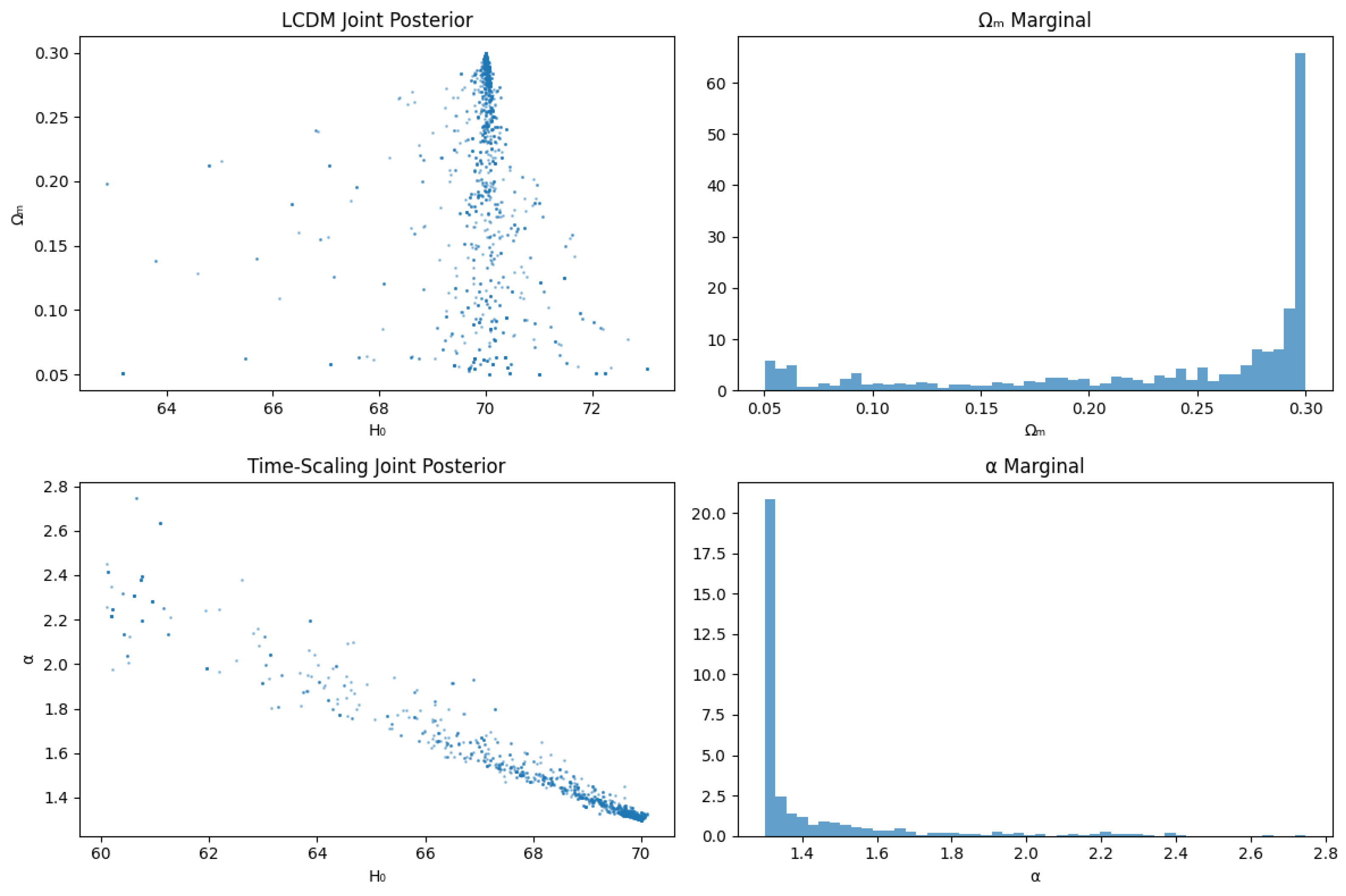
3.2. Posterior Sampling

To confirm that the best-fit points lie inside regions of high posterior probability, we ran a short affine-invariant Markov-Chain Monte Carlo analysis using supernova data only. The sampler used 64 walkers and 50 steps, initialized at the maximum-likelihood values from the supernova fits. Apart from broad top-hat priors— $50<H_0<100\mathrm{km}{\mathrm{s}}^{-1}{\mathrm{Mpc}}^{-1}$ and $0<{\mathrm{\Omega }}_m<1$ (or $0<\alpha <5$)—no additional constraints were imposed. Even this quick run on the supernova dataset reproduces the point estimates and spreads:

$$\begin{array}{cc}\hfill \Lambda \mathrm{CDM}:& H_0=69.94\pm 0.85,{\mathrm{\Omega }}_m=0.24\pm 0.08,\hfill \\ \hfill \mathrm{Time}--\mathrm{Scaling}:& H_0=68.89\pm 2.19,\alpha =1.42\pm 0.23,\hfill \end{array}$$

quoted as sample means ± one standard deviation.

As expected, the $\Lambda$CDM posterior is elongated—the familiar anti-correlation between $H_0$ and ${\mathrm{\Omega }}_m$. For the time-scaling model, most samples cluster tightly around $\alpha \simeq 1.4$, with a sharp drop-off and minimal tail beyond $\alpha \sim 1.7$.

The time-scaling model shows slightly larger uncertainty in $H_0$ but maintains tight constraints on the scaling parameter ($\alpha$). These features are illustrated in Figure 2.

3.3. Observed Trends

At low redshift, cosmic-chronometer (CC) data favor the $\Lambda$CDM model over the time-scaling model. Specifically, $\Lambda$CDM yields ${\chi }^2=14.55$, compared to ${\chi }^2=25.17$ for the time-scaling case, resulting in lower AIC and BIC scores. This is consistent with the fact that $\Lambda$CDM is explicitly constructed to fit late-time acceleration and that chronometer data are especially sensitive to this regime. However, residual systematics in stellar age dating—such as uncertainties in stellar population synthesis models or metallicity corrections—may bias these low-redshift fits and inflate the apparent preference for $\Lambda$CDM.

In the intermediate redshift range ($0.3\lesssim z\lesssim 2.3$), supernova data show nearly identical support for both models. The slight difference in ${\chi }^2$ values ($758.58$ for $\Lambda$CDM vs. $763.42$ for time-scaling) corresponds to minor shifts in AIC/BIC and lies within statistical uncertainty. This suggests that both frameworks—matter plus $\Lambda$ and power-law scaling—can adequately describe the expansion history inferred from standard candles over this redshift interval.

At high redshift ($z\gtrsim 2$), gamma-ray bursts yield ${\chi }^2=167.36$ for $\Lambda$CDM and ${\chi }^2=174.97$ for the time-scaling model. While this represents a modest numerical difference, it is not statistically significant. The similarity in fit quality implies that both models can track distance moduli effectively into the deep past, where data are sparse but increasingly critical for the resolution of tensions.

In the very-high-redshift regime probed by the CMB, the time-scaling model achieves a lower ${\chi }^2=83,939.46$, compared to (84,136.75) for $\Lambda$CDM. Despite having one extra parameter, it produces lower AIC/BIC values and fits the transformed Planck spectrum more closely. This performance arises partly from the adoption of a higher Hubble constant ($H_0=70.00$ km/s/Mpc) than the $\Lambda$CDM best fit ($H_0=67.19$), helping to bridge the gap between early- and late-time measurements.

When all four datasets are considered together, the time-scaling model outperforms $\Lambda$CDM by a wide margin. The total chi-squared is reduced by over 400,000, with ${\chi }_{\mathrm{red}}^2=51.612$ versus $143.538$, and the Akaike information criterion difference is $\Delta \mathrm{AIC}=401,254.37$. This strong statistical preference suggests that a single power-law exponent ($\alpha \simeq 1.06$) can effectively reproduce both late-time acceleration and early-universe structure without invoking a cosmological constant.

A key result is that for four datasets, the time-scaling model yields a Hubble constant near $H_0\simeq 70$ km/s/Mpc. This value lies between the CMB-inferred estimate (∼67) and the locally measured value from Cepheids and supernovae (∼73), suggesting that time scaling offers a potential compromise in Hubble tension. Posterior sampling confirms this trend: while $\Lambda$CDM shows a strong anti-correlation between $H_0$ and ${\mathrm{\Omega }}_m$, the time-scaling model tightly constrains the power-law exponent ($\alpha$) while allowing $H_0$ to vary more freely.

Crucially, both models remain statistically consistent with current observational uncertainties across all redshift ranges. Visual fits in Figure 1 confirm that the model curves generally lie within the error bars of the data points, indicating that differences in ${\chi }^2$ reflect subtle shape variations rather than gross mismatches.

In summary, $\Lambda$CDM remains statistically favored at low redshift (particularly in chronometer data), likely due to its explicit design to fit local acceleration. However, the time-scaling model shows stronger performance at high redshift; fits the CMB spectrum better; and achieves a consistent, intermediate value of $H_0$ across datasets. Thus, it represents itself as a computationally efficient and phenomenologically promising alternative to standard $\Lambda$CDM.

These empirical successes motivate a deeper examination of the dynamical origin of time scaling, prompting us to model $\alpha \left(t\right)$ as an evolving scalar degree of freedom coupled with curvature.

3.4. Scalar Field Dynamics

We compute ${\lambda }_L$ from the scalar subsystem because the background $(\alpha ,\dot{\alpha })$ phase space is effectively one-dimensional and does not support exponential divergence on its own. Thus, the scalar field provides the first meaningful degree of freedom capable of encoding time-directional instabilities.

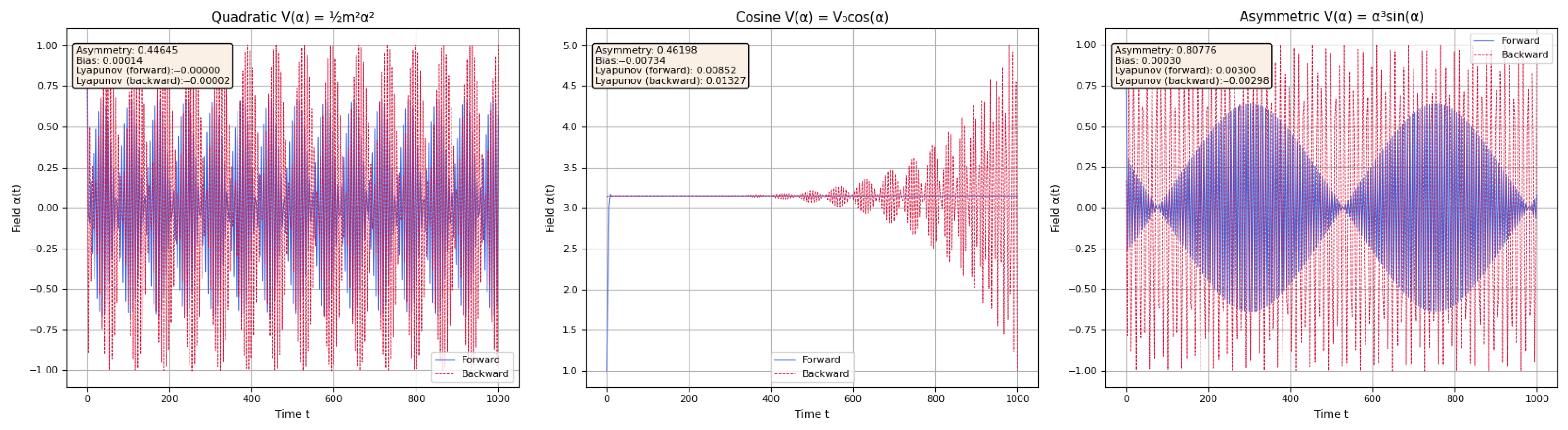
Both forward and backward numerical integration of Equation (22) is performed in time for the three potentials defined in Equations (23)–(25). Figure 3 displays the resulting field evolution, while Figure 4 quantifies trajectory divergence used to compute ${\lambda }_L$.

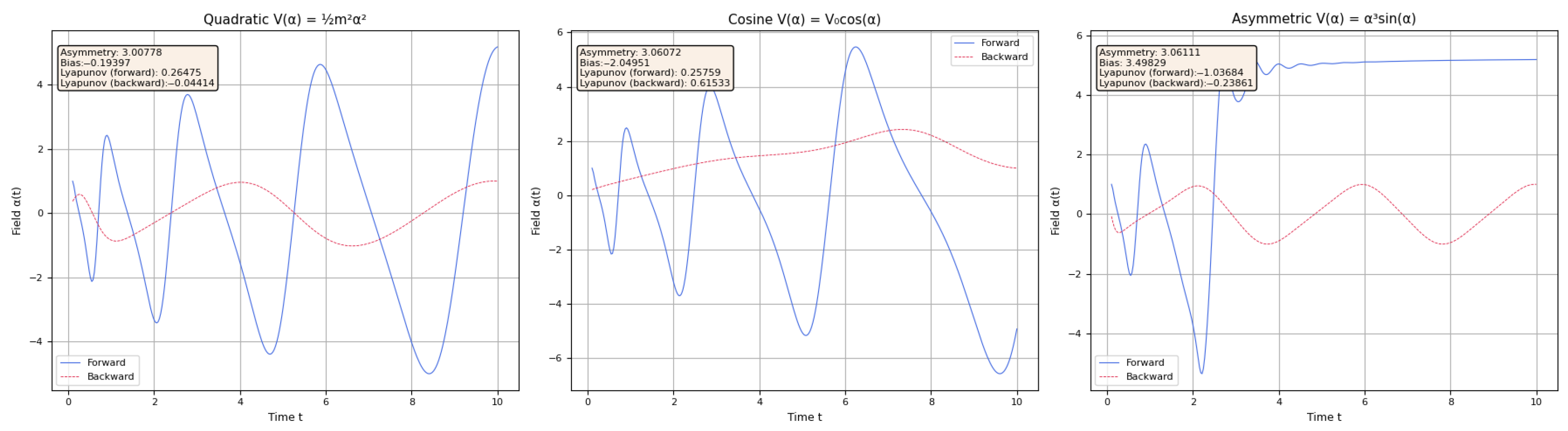
For the harmonic potential ($V\left(\alpha \right)=\frac{1}{2}{m}^2{\alpha }^2$), the field oscillates stably around the origin with constant amplitude. Both forward and backward solutions remain nearly identical, reflecting modest asymmetry ($\mathcal{A}\simeq 0.45$) and negligible bias ($\mathcal{B}\simeq 1.4\times {10}^{-4}$). The Lyapunov exponents in both directions are effectively zero (${\lambda }_L^{\mathrm{f},\mathrm{b}}\approx 0$), indicating fully reversible, non-chaotic evolution governed by symmetric curvature coupling.

In contrast, the cosine potential ($V\left(\alpha \right)=V_{0}cos\alpha$) produces a strongly asymmetric and weakly chaotic response. The forward solution quickly settles near a plateau at $\alpha \simeq 3.1$, while the backward trajectory exhibits exponential divergence, reaching values near 5. This yields significant asymmetry ($\mathcal{A}\simeq 0.46$) and positive Lyapunov exponents ($({\lambda }_L^{\mathrm{f}},{\lambda }_L^{\mathrm{b}})\simeq (0.0085,0.0133)$), indicating mild sensitivity to initial conditions. However, the bias remains small ($\mathcal{B}\simeq -0.007$), suggesting no net directional drift.

The third model, featuring the asymmetric potential ($V\left(\alpha \right)={\alpha }^{3}sin\alpha$), shows the strongest directional features. Forward and backward solutions diverge sharply: the forward trajectory becomes increasingly erratic, while the backward path displays damping and settles toward a regular plateau. This yields high asymmetry ($\mathcal{A}\simeq 0.808$), small bias ($\mathcal{B}\simeq 3\times {10}^{-4}$), and oppositely signed Lyapunov exponents ($({\lambda }_L^{\mathrm{f}},{\lambda }_L^{\mathrm{b}})\simeq (+0.0030,-0.0030)$). The signs here are notable: a positive ${\lambda }_L$ in the forward direction indicates weak instability, while a negative backward ${\lambda }_L$ suggests dynamical stability. In this sense, the model implies that time evolves from a more ordered past to a mildly chaotic future—consistent with the emergence of a thermodynamic arrow of time.

Physical Interpretation

The observed Lyapunov exponents, typically in the range of ${\lambda }_L\sim {10}^{-3}$, quantify the rate at which nearby scalar trajectories diverge or converge. Though small, these values signal weak (but non-negligible) sensitivity to initial conditions. Such slow-growing instabilities imply long-timescale chaotic dynamics that are insufficient to impact short-time observables but potentially relevant for the emergence of the cosmic arrow of time and entropy production. Unlike high-dimensional chaotic systems, the weak instability here is unlikely to produce practical unpredictability, yet it may contribute indirectly to cosmic structure or amplify early inhomogeneities. Notably, the asymmetric potential yields convergent dynamics in one direction (${\lambda }_L^{\mathrm{b}}<0$), suggesting an emergent arrow of time—even in the absence of dissipation.

3.5. Early Interval

To examine when temporal asymmetry becomes established, we re-integrate all three models over the early interval of $0<t<10$, as shown in Figure 5. Even in this short window, directional differences are evident. In the asymmetric case, the forward trajectory rapidly climbs and plateaus near $\alpha \approx 4.5$, while the backward path remains confined to low-amplitude oscillations.

The three models exhibit similar asymmetry values $\mathcal{A}\approx 3.06$, but the Lyapunov exponents and biases differ. The asymmetric potential shows forward convergence (${\lambda }_L^{\mathrm{f}}\approx -1.04$) and backward convergence (${\lambda }_L^{\mathrm{b}}\approx -0.24$), with large positive bias ($\mathcal{B}\approx +3.50$), suggesting directional settling onto a low-entropy attractor. The cosine potential shows chaotic growth in both directions (${\lambda }_L^{\mathrm{f}},{\lambda }_L^{\mathrm{b}}>0$), while even the symmetric quadratic case yields modest directional divergence, with ${\lambda }_L^{\mathrm{f}}\approx +0.26$ and a small negative backward exponent (${\lambda }_L^{\mathrm{b}}\approx -0.044$). This reflects scalar-curvature feedback, even in the absence of explicit parity breaking.

These findings imply that the arrow of time—in this scalar–tensor framework—is dynamically imprinted within the first few time units. It emerges not only from potential asymmetry but from the interaction between scalar dynamics and background geometry. Later evolution merely preserves the initial directionality, reinforcing the notion that cosmic time may reflect an early dynamical selection rather than a boundary condition.

Physical Interpretation

The directional behavior seen in the asymmetric model connects with earlier suggestions that the arrow of time reflects a highly ordered initial state [42,43]. These works argue that low gravitational entropy at the Big Bang sets the direction of time. In this view, the Big Bang is not treated as an explosion but as a kind of classical decoherence event or a transition from a highly constrained, symmetric configuration into a dynamically evolving state. In the present setup, time asymmetry emerges, instead, from classical scalar dynamics coupled with curvature. The asymmetric potential produces forward convergence (${\lambda }_L^{\mathrm{f}}<0$) and backward convergence, consistent with settling into a low-entropy attractor. This happens without dissipation or quantum input, indicating that mild parity breaking in the potential can act as a classical mechanism for time selection.

4. Discussion

This study set out to test whether a time-dependent expansion exponent ($\alpha \left(t\right)$) embedded in a scalar–tensor framework could reproduce key cosmological observables without invoking new fundamental physics. The numerical results confirm that such a setup can generate a classical arrow of time when the scalar potential breaks parity and fit high-redshift distance indicators (GRBs and the CMB-derived ${\mu }_{\mathrm{CMB}}$) competitively with $\Lambda$CDM while also presenting clear limitations at low redshift.

4.1. Theoretical Context

The scalar potentials explored in this work—quadratic, cosine, and parity breaking—represent a progression from symmetric to asymmetric field dynamics. These choices are motivated by well-established theoretical frameworks: the quadratic form appears in inflationary and quintessence models, the cosine potential resembles axion-like fields and pseudo-Nambu–Goldstone bosons with compactified moduli, and the parity-breaking ${\alpha }^{3}sin\alpha$ form acts as a minimal toy model capturing directional asymmetry. Since $\alpha \left(t\right)$ functions as a Brans–Dicke-type scalar, the setup belongs to the broader class of scalar–tensor and $f\left(R\right)$ theories. Similar couplings naturally arise in Kaluza–Klein reductions of higher dimensional gravity, reinforcing the idea that time-scaling dynamics may have geometric or symmetry-based origins. Importantly, the model invokes no exotic matter content or speculative physics: it reinterprets classical gravitational dynamics in a scalar–tensor framework with minimal assumptions.

4.2. Empirical Performance

Table 1 shows that the constant-$\alpha$ model stays within $\Delta \mathrm{AIC}\approx 7.6$ of $\Lambda$CDM for the GRB sample and improves upon it for the CMB data with $\Delta \mathrm{AIC}\approx -195.3$. For the full dataset of 4402 points, the time-scaling $\alpha \left(t\right)$ model yields a total of ${\chi }^2=225288.37$, compared to $626542.74$ for $\Lambda$CDM, resulting in a dramatic $\Delta \mathrm{AIC}=\Delta \mathrm{BIC}\approx 401254.37$. Both models show highly reduced ${\chi }^2$ values, indicating possible residual tensions or unaccounted-for systematics, but the time-scaling model provides a better overall fit to the data. In addition, the time-scaling approach offers significant computational advantages: it avoids nested numerical integrations and enables analytic evaluation of key observables such as $H\left(z\right)$ and $D_L\left(z\right)$, resulting in an approximately threefold speedup in likelihood evaluations. These features make it a useful control model for large-scale parameter scans and survey forecasts, even if its physical interpretation remains deliberately minimal.

4.3. Time Asymmetry

Figure 3, Figure 4 and Figure 5 indicate that scalar–curvature feedback can spontaneously select a preferred temporal direction, particularly when the potential lacks parity symmetry. This asymmetry develops within the first few time units ($t\lesssim 10$) and is quantified by divergent forward/backward trajectories and direction-dependent Lyapunov exponents. Interestingly, these features emerge in a purely classical context—without entropy production, quantum decoherence, or tuned initial conditions—highlighting how minimal extensions of the expansion law can imprint macroscopic time orientation in this toy model.

4.4. Practical Advantages

The model’s simplicity yields closed-form expressions for $H\left(z\right)$ and $D_L\left(z\right)$, avoiding nested numerical integration. For example, a test run with 64 MCMC walkers and 50 steps completed in $\sim 1$ min 30 s for $\Lambda$CDM but only $\sim 30$ s for the time-scaling model, reflecting the factor-three speed-up observed in routine likelihood calls. These gains make the framework a useful control case for probing data–model tensions and survey forecasts, particularly when computational cost is a concern.

4.5. Limitations and Future Work

This analysis addresses only the homogeneous background. A complete treatment must incorporate metric perturbations, re-analyze CMB anisotropies with Boltzmann codes, and verify post-Newtonian limits. The physical origin of the asymmetric scalar potential also remains to be explained—whether via spontaneous symmetry breaking, higher order curvature terms, or UV completion. Clarifying this origin is an important next step.

5. Conclusions

A single time-dependent power-law exponent offers a compact lens through which to examine persistent cosmological tensions and, in the present combined analysis, outperforms $\Lambda$CDM in global goodness of fit. High-redshift observations are matched with analytic tractability and reduced computational cost, while low-redshift data continue to favor the standard cosmological constant.

Embedding this framework in scalar–tensor gravity allows for a systematic extension to perturbation theory, where metric fluctuations and scalar-field perturbations must be treated jointly. In this context, $\alpha \left(t\right)$ represents the background scaling, while its perturbations enter the coupled dynamics alongside the usual scalar and tensor modes. Extending the analysis to include these perturbations—for example, via Boltzmann codes adapted to scalar–tensor dynamics—will allow full comparison with precision CMB and large-scale structure data.

Whether the expansion history is most economically described by a modified scale factor or by a coupled scalar field remains an open and testable question. In either case, the present approach provides a minimal and computationally efficient control model that can help isolate which features of the data truly require additional physics.