Abstract
Time series data are fundamental for analyzing temporal dynamics and patterns, enabling researchers and practitioners to model, forecast, and support decision-making across a wide range of domains, such as finance, climate science, environmental studies, and signal processing. In the context of high-dimensional time series, the Vector Autoregressive model (VAR) is widely used, wherein each variable is modeled as a linear combination of lagged values of all variables in the system. However, the traditional VAR framework relies on the assumption of stationarity, which states that the autoregressive coefficients remain constant over time. Unfortunately, this assumption often fails in practice, especially in systems subject to structural breaks or evolving temporal dynamics. The Time-Varying Vector Autoregressive (TV-VAR) model has been developed to address this limitation, allowing model parameters to vary over time and thereby offering greater flexibility in capturing non-stationary behavior. In this study, we propose an enhanced modeling approach for the TV-VAR framework by incorporating minimization solvers in generalized additive models and one-sided kernel smoothing techniques. The effectiveness of the proposed methodology is assessed using simulations based on non-homogeneous Markov chains, accompanied by a detailed discussion of its advantages and limitations. Finally, we illustrate the practical utility of our approach using an application to real-world financial data.
Keywords:
time-varying autoregressive model; generalized additive models; one-sided kernel smoothing; high-dimensional financial time series analysis MSC:
37M10
1. Introduction
The autoregressive (AR) model, as a versatile tool for analyzing and forecasting time series data, plays an important role in economics, weather forecasting, signal processing, and healthcare fields. In the application of the autoregressive model, the stationarity of time series data, in which the mean, variance, and autocovariance for the given processes remain constant over time, is one of the key assumptions. Unfortunately, in real-world scenarios, most signals and processes exhibit non-stationary behavior, which makes them unsuitable for AR modeling and can lead to systematic bias or inconsistent results [1]. Beyond signal processing, traditional risk models often rely on assumptions of stationarity and constant interdependencies, which are frequently violated during periods of market stress or structural shifts. In such turbulent conditions, asset correlations tend to rise sharply, a phenomenon known as correlation breakdown, resulting in a substantial underestimation of portfolio risk when using static or constant-parameter models. Thus, to effectively characterize such processes, it is essential to account for their non-stationary nature using either parametric or non-parametric models. Following this thought, one well-established approach in this context is the time-varying autoregressive (TV-AR) model, which is described in detail in [2]. In general, the framework of the TV-AR model with r time lags can be expressed as:
where is time-varying intercept, are time-varying parameters, and perturbation is zero-mean stationary process with , and for . In contrast to the AR model, the TV-AR model has a significant advantage in flexibility and adaptability due to its time-dependent parameters, making it more suitable for capturing non-stationary behavior and structural changes in time series data.
Next, in scenarios involving the investigation of complex internal relationships, where the internal relationship is non-negligible, the Vector Autoregressive (VAR) approach is employed as an efficient high-dimensional analytical method. However, as in the case of the AR model, the stationarity assumption is often violated in multivariate settings; therefore, the Time-Varying Vector Autoregressive (TV-VAR) model is employed as a multivariate framework to capture this temporal dynamics and interdependencies among multiple variables [3]. Typically, the TV-VAR model with r time lags can be expressed as:
where vector time series data , time-varying intercepts , time-varying matrix , and are independent samples drawn from a multivariate zero-mean stationary process with covariance matrix . Although TV-VAR models are widely used to capture non-stationary dynamics in multivariate time series, existing estimation approaches, such as local kernel smoothing and Time-Varying Parameter Bayesian VAR (TVP-BVAR), often lack explicit mechanisms for enforcing model stability. In particular, traditional methods do not directly control the stability of the time-varying process, despite its inherent tendency toward explosiveness in the absence of appropriate constraints. While TVP-BVAR is capable of estimating time-varying coefficients, its high computational cost and the complexity of modeling evolving parameters limit its practical applicability, particularly in high-dimensional or large-scale settings. In contrast, the generalized additive framework (GAM) and one-sided kernel smoothing (OKS) based frameworks adopted in this study offer more tractable and scalable alternatives for estimating time-varying dynamics with greater computational efficiency. Hence, in this study, we focus on modeling the TV-VAR process by incorporating the GAM- and OKS-based techniques, as proposed by [4]. We aim to enhance these methods by making the following contributions:
- We first derive recursive formulas to compute the expectation and covariance matrix of the TV-VAR process with r lags. These statistical properties serve as the foundation for reformulating the TV-VAR model as a constrained optimization problem. To ensure stable and reliable estimation of the time-varying coefficients, we conduct a detailed analysis of the underlying statistical structure and implement the solution using a numerical optimization framework in Python 3.9.
- In applying the generalized additive framework and kernel smoothing techniques, we further reformulate the TV-VAR optimization problem in a way that allows it to be solved using a variety of optimization methods.
- We present the performance results of our GAM-based and OKS-based methods using simulations of non-homogeneous Markov chains and discuss their respective strengths and limitations.
- Ultimately, our research suggests that non-stationary processes are better captured by a TV-VAR structure than traditional VAR models. Within both the GAM and OKS frameworks, gradient-based optimization algorithms incorporating stability constraints yield high performance in estimating time-varying coefficients.
The structure of the paper is as follows: Section 3 presents the recursive formulas for the mean and covariance, along with the corresponding optimization problems for three types of processes. Section 4 introduces the reformulated optimization framework, incorporating the generalized additive model and one-sided kernel smoothing techniques. Section 5 provides simulation results for four different scenarios of non-homogeneous Markov chains. Finally, Section 6 demonstrates the effectiveness of our approach using a finance-related dataset.
2. Literature Review
The Time-Varying Autoregressive model, as an extension of the AR model, offers non-negligible advantages in coefficient agility, making it highly suitable for non-stationary or structurally changing environments. Currently, TV-AR is widely used in psychology, for example, according to the research by [5,6], TV-AR shows a significant advantage in the study of psychology changing dynamics, especially for the emotion dynamics detection. In the research conducted by [7], the model was used to investigate potential changes of intra-individual dynamics in the perception of situations and emotions of individuals varying in personality traits. In addition to psychology, TV-AR is also widely used in fields such as finance and economics. For example, according to the research by [8], TV-AR can be used to examine how monetary policy jointly affects asset prices and the real economy in the United States. In the study conducted by [9], the TV-AR model was employed to quantify the economic and policy influences, capturing both regime-dependent and time-varying effects. In a study by [10], a TV-AR model was developed to analyze the effects of oil revenue on economic growth, providing empirical support for the resource curse hypothesis in Nigeria. Another area where TV-AR models are widely applied is engineering, including domains such as aerospace, mechanical systems, transportation, environmental monitoring, and infrastructure management. For example, in the research conducted by [11], a TV-AR model was developed to identify modal in structural health monitoring, and [12] used TV-AR to analyze the global or volcano seismological signals.
Compared to the AR model, when interdependencies among multiple variables are significant, the VAR model is a more effective approach for capturing autoregressive dynamics. For example, in the research conducted by [13], VAR was used to analyze the interrelationships between price spreads and the effects of wind forecast and demand forecast errors, and other exogenous variables. In the research conducted by [14], a Bayesian variant based VAR models was developed to forecast the international set of macroeconomic and financial variables. In the study conducted by [15], VAR was used to detect and analyze the relationships between two subgroups in eating behaviour, depression, anxiety, and eating control. However, as with the TV-AR model, incorporating time-varying parameters becomes essential when the assumption of stationarity is violated; hence, to accommodate both non-stationarity and inter-variable dynamics, the TV-VAR model provides a crucial extension. In practical applications, TV-AR and TV-VAR often share methodological similarities; however, TV-VAR places greater emphasis on modeling the dynamic interactions among variables. For example, in the field of psychology, the study by [16] demonstrated that time-varying parameters provide a robust framework for analyzing co-occurrence, synchrony, and the directionality of lagged relationships in real-world psychological data. Similarly, ref. [17] employed a TV-VAR model to examine the dynamics of automatically tracked head movements in mothers and infants, revealing temporal variations both within and across episodes of the Still-Face Paradigm. Furthermore, the research by [18] applied the TV-VAR model to capture complex multivariate interactions among psychological variables.
The TV-VAR model also plays a crucial role in the fields of economics and marketing. For instance, [19] employed a TV-VAR model to analyze the Japanese economy and monetary policy, uncovering their evolving structure over the period from 1981 to 2008. Similarly, ref. [20] used a TV-VAR framework to investigate the dynamic relationship between West Texas Intermediate crude oil and the U.S. S& P 500 stock market. In the context of stock market forecasting, ref. [21] demonstrated that the TV-VAR model holds significant potential for enhancing portfolio allocation strategies. Similarly, in the study by [22], the TV-VAR model was employed to analyze four types of oil price fluctuations: oil supply shocks, global demand shocks, domestic demand shocks, and oil-specific demand shocks. Additionally, ref. [23] applied this model to examine the dynamic interactions among economic policy uncertainty, investor sentiment, and financial stability. Further, ref. [24] used the TV-VAR model to explore return spillovers among major financial markets, including equity indices, exchange rates, Brent crude oil prices in the Asia-Pacific region, and the NASDAQ index. In addition to economic analysis, the TV-VAR model has also been widely applied in quantitative assessments of policy impacts, including analyses of monetary policy shocks [25], the effects of geopolitical risks and trade policy uncertainty [26], and international spillovers of US monetary policy [27].
3. Proposed Non-Stationary Process
In this section, the notation for the general stationary VAR model is first introduced, encompassing three different types of processes and their stochastic behavior. Subsequently, in the next section, the Generalized Additive Modeling (GAM-based) approach and the one-sided Kernel-smoothing (OKS-based) method are employed to estimate the parameters in the time-varying VAR models.
3.1. Time-Varying Autoregressive Model
In the TV-AR model with r lags, each observation at time t is predicted using the previous r observations, with time-varying coefficients that adjust to capture evolving dynamics. Overall, the TV-AR model is defined as:
where is reference time series data, represents the time-varying intercept, are time-varying parameters, and perturbation is a zero-mean stationary process with , and for . To estimate the mean value at time t, first define the mean value of TV-AR(r) at time t is , and assume the initial mean values are given, then use the mean recursive function to calculate :
Next, assume the covariance between time t and time is , so that:
In terms of , first assume , so that . Next, for , these terms can be expressed as the following recursive function:
Hence, can be computed recursively, and the covariance recursive function can be written as follows:
Take TV-AR(1) as an example, the expectation recursive function is given by:
The covariance recursive function is:
To estimate the time-varying parameters in (1), it is essential to assume smoothness along the time axis, which defines with the smoothness functions in time t. Next, define , and the recursive formulation implies that, for each iterations, if , then , As implied by the covariance recursion function, if the time-varying coefficient exceeds 1, as time t increase, the sequence becomes unstable and may diverge to infinity. This indicates that even a small initial error can propagate and amplify over time, resulting in substantial inaccuracies in future estimates. While such behavior is theoretically permissible in non-stationary processes, it introduces heightened sensitivity to initial conditions or early observations, which can substantially increase the risk of overfitting. Hence, to prevent covariance from exploding and to estimate the time-varying parameters , the TV-AR model can be reformulated and solved as the optimization problem (4).
where .
3.2. Vector Autoregressive Model
The VAR, one of the most fundamental multivariate time series analysis models, assumes that an p-dimensional time series vector can be expressed as:
where is a constant intercept vector, are the autoregressive coefficient matrices, and represents zero-mean multivariate Gaussian noise with covariance matrix . Compared to the TV-AR model, the stationary assumption is essential for VAR; thus, to compute its mean, the process is assumed to be weakly stationary, with a constant mean , and time-invariant covariances. Finally, the expectation is:
Next, assume the covariance between time t and time is , and the initial covariance functions where are given. Then:
By the definition of weak stationarity that , and . Then, the covariance recursive function is:
Finally, to estimate the stationary parameters in the VAR model (5), it is challenging to estimate the full coefficient matrix directly; therefore, a row-by-row estimation strategy is adopted. First, define , , thus, the row of stationary parameter can be estimated by solving optimization problem (8).
To solve this optimization problem, the simplest approach is to take the derivative of the objective function with respect to and set it equal to zero. Hence, the solution for is then given by:
3.3. Time-Varying Vector Autoregressive Models
The TV-VAR model, a non-stationary multivariate extension of VAR, allows the model parameters to vary over time, enabling dynamic adaptation to evolving relationships. In this framework, analogous to the TV-AR case, it is critical to assume smoothness along the time axis, as the process models a p-dimensional time series vector that evolves smoothly over time and can be expressed as:
where time-varying intercepts , time-varying matrix , and are independent samples drawn from a multivariate zero-mean stationary process with covariance matrix . Unlike VAR, weak stationarity does not hold in TV-VAR.in Thus, to calculate its mean value, first assume and the initial mean vectors are given, then the mean recursive function is given:
Next, to calculate the covariance function between time t and time is , assume the initial covariance functions where are given. Then:
Similar to TV-AR, can also be calculated recursively. Hence, the covariance recursive function is:
Next, to prevent the explosion of the covariance matrix, similar to the issue encountered in the TV-AR case, one of the most direct ways is to impose the constant constraint for each column m; in other words, the sum of the absolute values of each column across all time-varying parameter matrices is bounded by 1. Ultimately, estimating the time-varying coefficient matrix requires integrating the estimation approaches used in both the TV-AR and VAR models. First, define , . Thus, the row of time-varying parameter at time t, , is the solution of the optimization problem (12) under the sum constant constraint.
where . Finally, to solve the TV-VAR optimization problem (12), we introduce two approaches: one based on the Generalized Additive Model and the other on kernel smoothing techniques. These methods will be detailed in the following section.
4. Estimating Time-Varying Vector Autoregressive Model
In this section, we describe the estimation of the TV-VAR model using the GAM framework (e.g., as introduced in [28]), which accommodates non-linear relationships among variables. In addition to the GAM, we also consider a kernel smoothing approach, which estimates the time-varying coefficient matrices directly through kernel-weighted averaging, rather than relying on basis functions. The following subsections outline the training steps and overall workflow for implementing TV-VAR estimation using both the GAM and kernel smoothing methods.
4.1. Generalized Additive Model Workflow
The GAM is often introduced as a flexible extension of linear models, where smooth functions, referred to as smoothers, are added to capture non-linear patterns in the data. The core assumption of this approach is that the effect of each predictor on the response can be modeled by a smooth, non-parametric function rather than a fixed linear coefficient. This allows the model to capture complex relationships without requiring the analyst to predefine a specific functional form. The general structure of a GAM with n basis functions can be expressed as:
where represents a smooth basis function and represents the corresponding linear coefficient in the GAM framework. In this research, to estimate the time-varying coefficient matrices in a TV-VAR model with r lags, we assume the existence of r non-zero smooth functions to , each capturing the temporal variation of the corresponding lagged effect. Thus, the time-varying matrix and intercept vector under the GAM framework can be expressed as follows:
Next, to simplify the notation in time-varying matrix estimation, we make the following assumptions:
time value vector:
Time varying matrix:
where:
and coefficient bound vector:
Thus, the GAM-based TV-VAR coefficients can be calculated by solving the following optimization problem:
Finally, overparameterization is crucial when selecting basis functions, as it enables benign overfitting that enhances model flexibility without harming generalization. However, excessive flexibility can lead to malignant overfitting and unstable predictions [29,30]. Thus, a central challenge lies in choosing the appropriate type and number of basis functions. Common spline bases, such as cubic splines, B-splines, P-splines, and thin plate splines, offer distinct advantages for modeling shapes or surfaces with varying smoothness and flexibility requirements, spanning a continuum from moderately flexible (e.g., cubic and B-splines) to highly adaptive (e.g., P-splines and thin plate splines). However, the performance of spline-based models is highly sensitive to the number and placement of knots; suboptimal configurations can result in overfitting or underfitting. To mitigate these issues, data-driven approaches, such as adaptive splines and penalized splines, introduce mechanisms for automatic knot placement and smoothing parameter estimation, thereby enhancing model flexibility and reducing the need for manual tuning. However, these approaches often require the high cost of computational resources, particularly in high dimensions. Hence, beyond spline-based formulations, alternative basis functions, including exponential, linear, and Gaussian kernels, can be employed depending on the structural assumptions of the target function and the intended trade-offs between interpretability, smoothness, and computational efficiency. Therefore, in this study, we adopt splines alongside other selected basis functions, including Gaussian and tanh functions (a subset of the basis functions used in this study is shown in Figure 1).
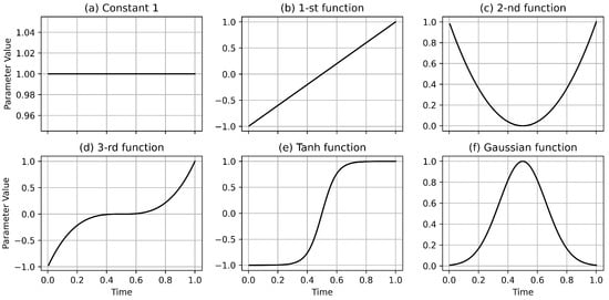
Figure 1.
Six different basis functions were used in the simulation study over the time interval . To ensure meaningful variation, the time variable t was scaled by a fixed constant in certain functions: specifically, t was multiplied by 5 in the Tanh function and by 2 in the Gaussian function. For the first, second, and third order basis functions, the time axis was first shifted by 0.5 and then scaled by a factor of 2 in the positive direction.
In the end, in the TV-VAR(r) model, after selecting the appropriate basis functions, a variety of strategies are available to solve the optimization problem (14) (The workflow of TV-VAR(1) is illustrated in Figure 2). One approach is to apply unconstrained regression methods such as ordinary linear regression, Lasso, or Ridge regression, though each comes with its limitations. For example, ordinary linear regression does not effectively enforce constraints, which can lead to an explosion in the covariance matrix and increasingly unstable predictions over time. In contrast, Lasso and Ridge regression address this issue by introducing a regularization term controlled by a tuning parameter , which governs the strength of the penalty and can be effectively selected via cross-validation [31].
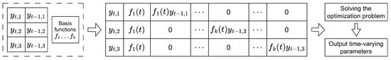
Figure 2.
One example of TV-VAR(1) with dimension amount .
Unfortunately, the traditional regression methods often fail to enforce constraints effectively; therefore, gradient-based optimization algorithms might be a more suitable alternative. Currently, several methods are available, including naive gradient descent, conjugate gradient, and the Broyden–Fletcher–Goldfarb–Shanno algorithm, all of which can handle both constrained and unconstrained optimization. However, for those algorithms, constrained nonlinear optimization problems can sometimes be time-consuming and might cause malignant overfitting. Hence, to address such linear constraints in optimization problem (14), in this research, we employ a Lagrangian gradient-based solver (from the Python SciPy package, named ’trust-constr’ model).
4.2. Kernel Smoothing Method Based Workflow
Kernel smoothing (KS), a non-parametric method for estimating unknown functions, is commonly used to evaluate time-varying parameters by fitting and combining a sequence of local models across different time points in the series. Similar to GAM, KS also assumes that the effects of predictor variables can be smoothly captured by non-parametric functions. In the KS model, the bandwidth parameter b plays a critical role, which should be small enough to capture the time-varying structure of the underlying model. However, if b is too small, the algorithm may become overly sensitive to local fluctuations, leading to overfitting. Typically, the KS weight at time is given by:
where t denotes a time point in the series, is the target time at which the time-varying parameter matrix is to be estimated, and b is the bandwidth parameter that controls the degree of smoothness in the estimation. Next, to estimate the time-varying coefficient matrix in the TV-VAR(r) model using the KS approach, the weighted optimization problem is used in place of the original optimization problem (12). However, in the standard KS model, where the time typically ranges from r to the final time T, when estimating parameters for times between and T, the model may inadvertently incorporate information from the “future” observations, data points occurring after the target time, potentially introducing look-ahead bias in certain applications. Therefore, this research applied the one-sided kernel smooth (OKS) method, which forces the final time T to be , and its optimization problem is given as (15).
Traditionally, the minimization problem in Equation (15) admits a solution; however, this solution does not necessarily satisfy the required constraints. Therefore, to effectively solve the optimization problem, we reformulate it into an equivalent problem that can be solved numerically, similar to the approach used in the GAM case. Before proceeding with the numerical solver, to clarify the notation, here are some necessary assumptions:
Time value vector:
Time varying matrix:
where:
and coefficient bound vector:
Thus, the OKS-based TV-VAR coefficients at time can be calculated by (16), and the workflow of this method is shown in Figure 3.
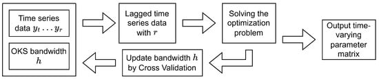
Figure 3.
Working flow of TV-VAR with OKS method.
Finally, the critical step is selecting the bandwidth b. As noted earlier, increasing the bandwidth b incorporates more data into the estimation around a given point, but if b is too large, it may lead to underfitting by oversmoothing the data and obscuring local patterns. In contrast, a bandwidth that is too small may result in overfitting by capturing noise instead of the underlying structure. In the study by [32], several strategies were proposed to select an appropriate bandwidth. Among these, cross-validation was identified as the most suitable for our context and is therefore employed in this research to determine the optimal bandwidth. In the end, similar to the GAM framework, the optimization problem is solved using a gradient-based method, specifically, the Lagrange gradient descent implemented with the publicly available SciPy package.
5. Evaluating Performance via Simulation
In this section, we present our simulation studies based on non-homogeneous Markov chains to evaluate the performance of the proposed methods in practical scenarios. The non-homogeneous Markov chain is a stochastic process in which the transition probabilities vary over time, in contrast to a homogeneous Markov chain, where the transition probabilities remain fixed and independent of the time step. In real-world applications, this type of Markov chain is widely used for mathematical modeling, simulation, and analysis of complex systems with uncertain or evolving dynamics, particularly in network analysis across various fields, including social sciences, environmental sciences, bioinformatics, and finance [33,34,35]. Specifically, this research investigates two approaches to modeling non-homogeneous Markov chains: the first employs a transition matrix that evolves smoothly and continuously over time without an intercept term, while the second introduces an additional time-varying constant to capture subtle dynamic variations. Accordingly, the primary process for generating the second-order time-varying test data is defined as follows:
where denotes a time-varying intercept, and are time-varying coefficient matrices, is a Gaussian noise vector with zero mean and covariance , and is a scalar controlling the noise magnitude. Subsequently, to evaluate the performance of our TV-VAR–based methods, the mean absolute error (MAE), as defined in Equation (17), is computed over a forecast horizon of length H. Initially, two additional evaluation metrics, Mean Absolute Percentage Error (MAPE) and Root Mean Squared Error (RMSE), were considered for performance assessment. However, the presence of values approaching zero in some test cases led to numerical instability in MAPE, thereby undermining its reliability. Furthermore, the differences between RMSE and MAE were consistently minimal, suggesting that RMSE provided limited additional analytical value beyond what was captured by MAE. Therefore, this study focuses exclusively on MAE as the primary evaluation metric.
For the GAM-based approach, the time-varying coefficient matrix, constructed using basis functions, was estimated from past data and then used to predict the values for the next H time steps, with the corresponding prediction error calculated. In contrast, the OKS method assumed a fixed coefficient matrix over the forecast horizon, and predictions were made under this assumption, followed by evaluation of the resulting prediction error. All simulations in this study were conducted using Python, with the source code and related datasets available as detailed in the Data Availability Statement.
5.1. Simulation Preparation
For the case of a transition matrix that changes smoothly over time without time-varying intercepts, we consider the following specific scenarios:
- Scenario 1: consider a zero-intercept time-series data with dimension , where the initial value is set to , a small noise scaling parameter which fixed to , and the Gaussian noise covariance matrix . The time-varying coefficient matrix is initialized as a uniform random matrix, normalized row-wise to form a row-stochastic matrix, and updated using the following functions:
- Using the same initial value, noise scaling parameter, and strategy for generating the initial time-varying coefficient matrix as in Scenario 1, but with an increased dimension , the Gaussian noise covariance matrix , and the new time-varying coefficient matrix update function, which is defined as follows:
Next, a small time-varying intercept is introduced in Scenarios 1 and 2 to enhance the dynamic behavior and evaluate the model performance. In addition to the prediction analysis, to better analyze the performance of the TV-VAR model in visualization, we apply the GAM in multiple cases of Scenarios 1 and 3 to reconstruct the whole process, as the stationarity and local stationarity assumptions of VAR and OKS make them unsuitable for this type of visualization. Specifically, we consider a time series consisting of 200 data points, with the first 180 used for training and the remaining 20 reserved for prediction. For visualization analysis, after estimating the time-varying coefficient matrices using GAM, we feed the first r lag values into the model and let it recursively estimate the remaining data points. The initial time-varying coefficient matrix is defined below:
5.2. Simulation Results
For each scenario, the predictions are made two steps ahead using 100 randomly generated time series samples, each of length 200, with time t normalized from 0 to 1, and the performance is evaluated using MAE across these steps. In this study, we implement the examples using GAM, OKS, traditional Vector Autoregressive (VAR) models (estimated via matrix-based updates), and L-VAR (with coefficients estimated through Lasso regression) with lags and . The results for the two scenarios without an intercept are shown in Table 1 and Table 2, while the results for the scenarios, including MAE, mean, sample variance (SV), and minimum (Min) and maximum (Max) values, with time-varying intercepts are presented in Table 3 and Table 4. Next, the reconstructed results of the GAM-based method are shown in Figure 4. Finally, to evaluate the processing time of the GAM- and OKS-based methods across different time series dimensions, we ran each method 50 times per dimension under Scenario 1. The average processing time is presented in Table 5.

Table 1.
The summary statistics of absolute errors across 100 random samples in Scenario 1.
Table 2.
The summary statistics of absolute errors across 100 random samples in Scenario 2.
Table 3.
The summary statistics of absolute errors across 100 random samples in Scenario 3.
Table 4.
The summary statistics of absolute errors across 100 random samples in Scenario 4.
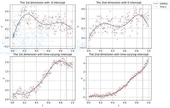
Figure 4.
Two examples of time-varying series data by using GAM(2), where the time-varying intercept is defined as .
Table 5.
Computational time for the GAM- and OKS-based methods across different dimensions p.
5.3. Discussion
The simulation results above compare the prediction performance of GAM, OKS, and VAR in modeling non-homogeneous Markov chains, both with and without an intercept. As expected, the MAE generally increases as the forecast horizon H extends from 1 to 2. In scenarios with stronger time-varying dynamics, both GAM and OKS outperform VAR and L-VAR, which aligns with our hypothesis, given that VAR and L-VAR assume stationarity in the whole process. However, OKS performs worse than GAM because it assumes that the estimated time-varying coefficient matrix remains fixed after the prediction point, which limits its adaptability, especially in situations where the coefficient matrix changes dramatically over time. Next, the performance of the GAM(2) model appears less effective in the zero-intercept setting compared to the non-zero intercept case. This is because, in processes with non-zero intercepts, the influence of time-varying effects tends to diminish in significance, thereby allowing even a stationary VAR model to achieve satisfactory performance. Furthermore, when reconstructing the entire time series, neither VAR nor OKS is suitable due to their reliance on stationarity assumptions; VAR assumes global stationarity, while OKS relies on local stationarity. As a result, they are only capable of forecasting or simulating specific time points, rather than capturing the full dynamic process. Finally, to evaluate robustness with respect to input length, we assessed the performance of both the GAM- and OKS-based models across time series ranging from 50 to 200 observations, and found their performance to be largely insensitive to series length. This insensitivity is likely due to the short forecasting horizon, a fixed two-step-ahead prediction, which limits temporal dependency and thereby reduces the influence of the overall input length on predictive accuracy.
Unfortunately, both our GAM-based and OKS-based methods require significantly more coefficients compared to traditional VAR, leading to increased computational complexity and higher time costs, which can limit overall performance. For example, consider a vector time series with dimension , and assume five different basis functions. In the case of a second-order model, GAM(2) requires estimating coefficients, similarly, OKS(2) requires coefficients. Next, the time complexity of the proposed approach largely depends on the choice of optimization algorithm and the computational hardware used. In this study, we employed the ’trust-constr’ algorithm from the SciPy package, which utilizes Lagrangian gradient descent to handle constrained optimization. While switching to a faster algorithm, such as ’L-BFGS-B’, may reduce computation time, it generally lacks support for constraints, potentially compromising solution feasibility. Specifically, all experiments were conducted on a system equipped with an NVIDIA RTX 3060 GPU. Under this setup, training the GAM-based method with a lag order of one required approximately 2 to 71 s, depending on the time series dimension. When the lag order increased to two, the per-sample training time rose to approximately 3 to 144 s, reflecting the increased model complexity. Additionally, the OKS-based method exhibited a distinct trend. Although significantly slower than GAM at lower dimensions, due to the additional computation required for cross-validation, it became substantially more efficient at higher dimensions. In contrast, although VAR requires matrix inversion operations, it remains significantly faster than both GAM and OKS in practice. Overall, increasing the number of lags enables the model to capture longer-term dependencies and reveal stronger connections within the time series, potentially improving forecast performance, but it also significantly increases parameter complexity and the risk of overfitting. Therefore, effectively applying TV-VAR models requires a careful balance between model complexity and the number of lags to capture temporal dependencies without overfitting.
6. Estimating Time-Varying VAR Model on Finance-Related Datasets
In the real-world application, we consider the time series data in the finance domain, incorporating some key market indicators, including the S&P 500 index (as a broad measure of U.S. equity market performance), the VIX index (reflecting market volatility and investor sentiment), and U.S. Treasury securities with a one-month constant maturity (serving as a proxy for short-term interest rates and risk-free returns). In this research, all financial data were obtained from publicly available sources, including the Federal Reserve Economic Data at https://fred.stlouisfed.org/ (accessed on 1 May 2025) and the Chicago Board Options Exchange at https://www.cboe.com/ (accessed on 1 May 2025). These indices are widely used in financial modeling and risk assessment due to their relevance in capturing market dynamics, investor behavior, and macroeconomic conditions.
6.1. Data Preparation
Before modeling, several preprocessing steps are essential. For the S&P 500 index, prior research has traditionally focused on various forms of returns, such as simple and logarithmic returns, based on the assumption of stationarity. While this return-based approach facilitates certain statistical modeling techniques, it may overlook important information embedded in the actual index levels, making such models less effective in accurately predicting future price levels. Hence, to address this limitation, this study instead focuses on modeling the index itself rather than its derived returns. Next, occasional breakpoints in the one-month constant maturity series, caused by sudden shifts in market conditions or expectations, such as spikes in volatility, changes in monetary policy, or other technical factors, are filled using the value from the preceding day. The data used in this study were collected for the period spanning 4 January 2016 to 31 December 2024.
6.2. Results
To evaluate the performance of our methods on real-world financial data, we use the period from 4 January 2016 to 28 June 2024, to train the TV-VAR model under both the GAM and OKS frameworks with a lag order of . After that, we perform one-step-ahead forecasting and compare the predicted values with the actual observations, denoted as , which is then fed back into the model to retrain both GAM and OKS for the next prediction step. The complete prediction results, including the mean absolute error, are presented in Figure 5 and Table 6.
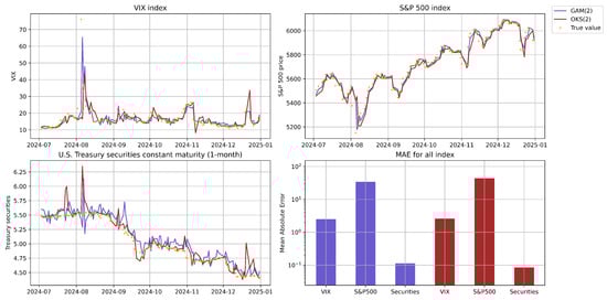
Figure 5.
Prediction results related to VIX, S&P 500, and U.S. Treasury securities with a 1-month constant maturity with the time from 4 January 2016 to 31 December 2024.
Table 6.
The summary statistics of absolute errors in the real-world financial data.
The results show that both GAM and OKS perform well, achieving low MAEs across all three indices, although GAM exhibits slightly more fluctuation than OKS in predicting U.S. Treasury securities. Additionally, the findings suggest that when the VIX is high, U.S. Treasury securities tend to decline the following day. This aligns with expectations, as high market volatility often drives investors toward safe-haven assets, such as Treasury bonds, which in turn affects yields. Conversely, when the VIX decreases, investors tend to reallocate capital into equities such as the S&P 500, leading to reduced demand for Treasuries. Finally, the relationship between the VIX and the S&P 500 also holds: when the VIX is elevated, the S&P 500 typically declines or exhibits only modest gains, consistent with established market behavior.
7. Conclusions
Compared to stationarity, non-stationarity—where a time series’ statistical properties change over time—better aligns with real-world dynamics in fields such as finance, climate science, healthcare, and signal processing. Failing to account for it may lead to poor forecasts, especially in long-term predictions. The autoregressive model, a foundational tool in time series analysis, plays a crucial role in modeling time-dependent data, and its extension, the time-varying vector autoregressive (TV-VAR) model, broadens this framework to effectively handle both non-stationary dynamics and high-dimensional settings. Recent research on TV-VAR models has highlighted the effectiveness of the generalized additive model (GAM) framework and kernel smoothing (KS) methods in capturing dynamic relationships. However, few studies explicitly consider the case of TV-VAR with r lags. To model this process efficiently, we reformulate it as a series of optimization problems under appropriate constraints, which preserves the covariance structure between predictions and historical data without overfitting it over time. The methods presented in this research model TV-VAR time series data using optimization solvers, and simulation results demonstrate a clear advantage in prediction accuracy, especially under strong time variation. Furthermore, compared to the stationary VAR model and the OKS method, the GAM-based model not only delivers significantly better predictive performance but also enables reconstruction of the entire training process from the initial r lags, providing enhanced interpretability and flexibility. Compared to traditional hedging strategies, which assume stationarity, the TV-VAR framework offers significant advantages by capturing time-varying relationships and enabling the implementation of adaptive hedge ratios. In other words, when the model detects increased portfolio sensitivity to shocks or rising market volatility, it can trigger more proactive hedging with appropriate instruments, an adaptability that is especially crucial for managing tail risk, where sudden market shifts require swift and responsive adjustments.
As with other studies, our approaches—both GAM-based and OKS-based—have certain limitations. The primary drawback is the large number of parameters that must be estimated, especially in models with high dimensionality and many lags, making the model’s performance highly dependent on the efficiency of the optimization solver and susceptible to accuracy loss in the presence of high data noise. Hence, future research could explore two potential directions: first, reconstructing the GAM-based model using neural networks, particularly physics-informed neural networks, by integrating the time-varying framework in TV-VAR with physical constraints to enhance model structure and interpretability; second, refining the bandwidth selection for the OKS method, as the current cross-validation approach is time-consuming, and developing a more efficient method could significantly enhance its effectiveness. Therefore, our future work will involve reformulating the TV-VAR model with physics-based constraints and integrating it with deep learning techniques.
Author Contributions
Z.J.: conceptualized and designed the study, formulated all algorithms, and wrote the manuscript. W.L. helped with the data analysis. Y.J. and X.L. contributed to the interpretation of the results. All authors have read and agreed to the published version of the manuscript.
Funding
This research received no external funding.
Data Availability Statement
The data and code used in this study are available on GitHub at https://github.com/zhixuan1994/Time-Varying-Autoregressive-Model.git (accessed on 5 June 2025) for purposes of replication and further research. Additionally, they will be deposited in a publicly accessible repository upon publication to ensure transparency and facilitate broader access to the research community.
Conflicts of Interest
The authors declare no conflict of interest.
References
- Baptista de Souza, D.; Kuhn, E.V.; Seara, R. A Time-Varying Autoregressive Model for Characterizing Nonstationary Processes. IEEE Signal Process. Lett. 2019, 26, 134–138. [Google Scholar] [CrossRef]
- Hamilton, J.D. Time Series Analysis; Princeton University Press: Princeton, NJ, USA, 1994. [Google Scholar]
- Jiang, X.Q.; Kitagawa, G. A time varying coefficient vector AR modeling of nonstationary covariance time series. Signal Process. 1993, 33, 315–331. [Google Scholar] [CrossRef]
- Haslbeck, J.M.B.; Waldorp, L.J. mgm: Estimating Time-Varying Mixed Graphical Models in High-Dimensional Data. J. Stat. Softw. 2020, 93, 1–46. [Google Scholar] [CrossRef]
- Bringmann, L.F.; Hamaker, E.L.; Vigo, D.E.; Aubert, A.; Borsboom, D.; Tuerlinckx, F. Changing dynamics: Time-varying autoregressive models using generalized additive modeling. Psychol. Methods 2017, 22, 409–425. [Google Scholar]
- Bringmann, L.F.; Ferrer, E.; Hamaker, E.L.; Borsboom, D.; Tuerlinckx, F. Modeling Nonstationary Emotion Dynamics in Dyads using a Time-Varying Vector-Autoregressive Model. Multivar. Behav. Res. 2018, 53, 293–314. [Google Scholar] [CrossRef] [PubMed]
- Casini, E.; Richetin, J.; Preti, E.; Bringmann, L.F. Using the time-varying autoregressive model to study dynamic changes in situation perceptions and emotional reactions. J. Personal. 2020, 88, 806–821. [Google Scholar] [CrossRef]
- Paul, P. The Time-Varying Effect of Monetary Policy on Asset Prices. Rev. Econ. Stat. 2020, 102, 690–704. [Google Scholar] [CrossRef]
- Pleșa, G. State-Dependent and Time-Varying Effects of Monetary Policy. Eastern Eur. Econ. 2025, 0, 1–24. [Google Scholar] [CrossRef]
- Olayungbo, D. Effects of oil export revenue on economic growth in Nigeria: A time varying analysis of resource curse. Resour. Policy 2019, 64, 101469. [Google Scholar] [CrossRef]
- Yao, X.J.; Yi, T.H.; Qu, C.X. Autoregressive spectrum-guided variational mode decomposition for time-varying modal identification under nonstationary conditions. Eng. Struct. 2022, 251, 113543. [Google Scholar] [CrossRef]
- Tary, J.B.; Herrera, R.H.; van der Baan, M. Time-varying autoregressive model for spectral analysis of microseismic experiments and long-period volcanic events. Geophys. J. Int. 2013, 196, 600–611. [Google Scholar] [CrossRef]
- Spodniak, P.; Ollikka, K.; Honkapuro, S. The impact of wind power and electricity demand on the relevance of different short-term electricity markets: The Nordic case. Appl. Energy 2021, 283, 116063. [Google Scholar] [CrossRef]
- Cuaresma, J.C.; Feldkircher, M.; Huber, F. Forecasting with Global Vector Autoregressive Models: A Bayesian Approach. J. Appl. Econom. 2016, 31, 1371–1391. [Google Scholar] [CrossRef]
- Wild, B.; Eichler, M.; Friederich, H.C.; Hartmann, M.; Zipfel, S.; Herzog, W. A graphical vector autoregressive modelling approach to the analysis of electronic diary data. BMC Med. Res. Methodol. 2010, 10, 28. [Google Scholar]
- Van der Does, F.; van Eeden, W.; Bringmann, L.F.; Lamers, F.; Penninx, B.W.J.H.; Riese, H.; Vermetten, E.; van der Wee, N.; Giltay, E. Dynamic time warp versus vector autoregression models for network analyses of psychological processes. Sci. Rep. 2025, 15, 11720. [Google Scholar]
- Chen, M.; Chow, S.M.; Hammal, Z.; Messinger, D.S.; Cohn, J.F. A Person- and Time-Varying Vector Autoregressive Model to Capture Interactive Infant-Mother Head Movement Dynamics. Multivar. Behav. Res. 2021, 56, 739–767. [Google Scholar] [CrossRef] [PubMed]
- Scholten, S.; Rubel, J.A.; Glombiewski, J.A.; Milde, C. What time-varying network models based on functional analysis tell us about the course of a patient’s problem. Psychother. Res. 2025, 35, 637–655. [Google Scholar] [CrossRef] [PubMed]
- Nakajima, J.; Kasuya, M.; Watanabe, T. Bayesian analysis of time-varying parameter vector autoregressive model for the Japanese economy and monetary policy. J. Jpn. Int. Econ. 2011, 25, 225–245. [Google Scholar] [CrossRef]
- Lu, F.; Qiao, H.; Wang, S.; Lai, K.K.; Li, Y. Time-varying coefficient vector autoregressions model based on dynamic correlation with an application to crude oil and stock markets. Environ. Res. 2017, 152, 351–359. [Google Scholar] [CrossRef]
- Gupta, R.; Huber, F.; Piribauer, P. Predicting international equity returns: Evidence from time-varying parameter vector autoregressive models. Int. Rev. Financ. Anal. 2020, 68, 101456. [Google Scholar] [CrossRef]
- Chen, J.; Zhu, X.; Li, H. The pass-through effects of oil price shocks on China’s inflation: A time-varying analysis. Energy Econ. 2020, 86, 104695. [Google Scholar] [CrossRef]
- Qi, X.Z.; Ning, Z.; Qin, M. Economic policy uncertainty, investor sentiment and financial stability—An empirical study based on the time varying parameter-vector autoregression model. J. Econ. Interact. Coord. 2022, 17, 779–799. [Google Scholar] [PubMed]
- Sarathkumara, S.M.N.N.; Samarakoon, S.M.R.K.; Pradhan, R. Navigating financial interconnectivity: Analyzing oil, exchange rates and US market influences on Asia-Pacific equities using the time-varying parameter vector autoregressive connectedness approach. J. Econ. Stud. 2025. ahead-of-print. [Google Scholar]
- Roşoiu, A. Monetary Policy and Time Varying Parameter Vector Autoregression Model. Procedia Econ. Financ. 2015, 32, 496–502. [Google Scholar] [CrossRef]
- Yang, C.; Niu, Z.; Gao, W. The time-varying effects of trade policy uncertainty and geopolitical risks shocks on the commodity market prices: Evidence from the TVP-VAR-SV approach. Resour. Policy 2022, 76, 102600. [Google Scholar] [CrossRef]
- Crespo Cuaresma, J.; Doppelhofer, G.; Feldkircher, M.; Huber, F. Spillovers from Us Monetary Policy: Evidence from a Time Varying Parameter Global Vector Auto-Regressive Model. J. R. Stat. Soc. Ser. A Stat. Society 2019, 182, 831–861. [Google Scholar] [CrossRef]
- Hastie, T.J. Statistical Models in S; Routledge: Abingdon, UK, 2017. [Google Scholar]
- Bartlett, P.L.; Long, P.M.; Lugosi, G.; Tsigler, A. Benign overfitting in linear regression. Proc. Natl. Acad. Sci. USA 2020, 117, 30063–30070. [Google Scholar] [CrossRef]
- Shamir, O. The Implicit Bias of Benign Overfitting. In Proceedings of the Thirty Fifth Conference on Learning Theory, London, UK, 2–5 July 2022; Loh, P.L., Raginsky, M., Eds.; Proceedings of Machine Learning Research; PMLR: Birmingham, UK, 2022; Volume 178, pp. 448–478. [Google Scholar]
- Friedman, J.H.; Hastie, T.; Tibshirani, R. Regularization Paths for Generalized Linear Models via Coordinate Descent. J. Stat. Softw. 2010, 33, 1–22. [Google Scholar] [CrossRef]
- Köhler, M.; Schindler, A.; Sperlich, S. A Review and Comparison of Bandwidth Selection Methods for Kernel Regression. Int. Stat. Rev. 2014, 82, 243–274. [Google Scholar] [CrossRef]
- Guarino, S.; Mastrostefano, E.; Celestini, A.; Bernaschi, M.; Cianfriglia, M.; Torre, D.; Zastrow, L.R. A Model for Urban Social Networks. In Proceedings of the Computational Science–ICCS 2021, Krakow, Poland, 16–18 June 2021; Paszynski, M., Kranzlmüller, D., Krzhizhanovskaya, V.V., Dongarra, J.J., Sloot, P.M., Eds.; Springer International Publishing: Cham, Switzerland, 2021; pp. 281–294. [Google Scholar]
- Gallegos-Herrada, M.A.; Rodrigues, E.R.; Tarumoto, M.H.; Tzintzun, G. A multi-dimensional non-homogeneous Markov chain of order K to jointly study multi-pollutant exceedances. Environ. Ecol. Stat. 2023, 30, 157–187. [Google Scholar]
- Chang, J.; Chan, H.K.; Lin, J.; Chan, W. Non-homogeneous continuous-time Markov chain with covariates: Applications to ambulatory hypertension monitoring. Stat. Med. 2023, 42, 1965–1980. [Google Scholar] [CrossRef] [PubMed]
Disclaimer/Publisher’s Note: The statements, opinions and data contained in all publications are solely those of the individual author(s) and contributor(s) and not of MDPI and/or the editor(s). MDPI and/or the editor(s) disclaim responsibility for any injury to people or property resulting from any ideas, methods, instructions or products referred to in the content. |
© 2025 by the authors. Licensee MDPI, Basel, Switzerland. This article is an open access article distributed under the terms and conditions of the Creative Commons Attribution (CC BY) license (https://creativecommons.org/licenses/by/4.0/).