A Bayesian Additive Regression Trees Framework for Individualized Causal Effect Estimation

Abstract

In causal inference research, accurate estimation of individualized treatment effects (ITEs) is at the core of effective intervention. This paper proposes a dual-structure ITE-estimation model based on Bayesian Additive Regression Trees (BART), which constructs independent BART sub-models for the treatment and control groups, estimates ITEs using the potential outcome framework and enhances posterior stability and estimation reliability through Markov Chain Monte Carlo (MCMC) sampling. Based on psychological stress questionnaire data from graduate students, the study first integrates BART with the Shapley value method to identify employment pressure as a key driving factor and reveals substantial heterogeneity in ITEs across subgroups. Furthermore, the study constructs an ITE model using a dual-structured BART framework (BART-ITE), where employment pressure is defined as the treatment variable. Experimental results show that the model performs well in terms of credible interval width and ranking ability, demonstrating superior heterogeneity detection and individual-level sorting. External validation using both the Bootstrap method and matching-based pseudo-ITE estimation confirms the robustness of the proposed model. Compared with mainstream meta-learning methods such as S-Learner, X-Learner and Bayesian Causal Forest, the dual-structure BART-ITE model achieves a favorable balance between root mean square error and bias. In summary, it offers clear advantages in capturing ITE heterogeneity and enhancing estimation reliability and individualized decision-making.

1. Introduction

In recent years, the rapid expansion of graduate education in China has been accompanied by a significant rise in psychological pressure among graduate students. This growing burden stems from a confluence of factors, including the demands of academic research, employment uncertainty and financial strain. As a result, the prevalence of mental health issues—such as depression and anxiety—has steadily increased year over year [1,2]. Given the multifaceted nature of psychological stress, traditional statistical approaches such as linear or logistic regression often fall short in capturing the complex, nonlinear relationships and interaction effects among contributing variables. This limitation hinders the accurate identification of key driving factors [3]. Furthermore, in assessing the impact of psychological interventions, most existing studies emphasize the average treatment effect (ATE), while neglecting individual-level variation in treatment response—referred to as the individualized treatment effect [4,5,6]. This oversight poses a significant barrier to designing personalized intervention strategies for graduate students facing varying levels of psychological risk.

In the study of inference, accurately estimating ITE remains a thorny problem. Traditional methods such as probability score matching (PSM) [7] and dual-estimation probability estimation generally perform poorly in high-dimensional and nonlinear environments [8,9]. In recent years, machine learning methods have generally performed poorly in complex data modeling [10,11]. BART has attracted much attention due to its advantages, and BART has shown good prospects in the field of causal inference with its powerful nonparametric modeling capabilities and uncertainty-quantification characteristics [12,13]. However, the application of existing BART in ITE analysis is still relatively limited, especially in the deep mining of structural modeling and individual heterogeneity identification.

To address the above issues, this paper proposes a dual-structure individualized causal effect-estimation model based on BART, namely the BART-ITE model. This model innovatively introduces treatment variables into the BART framework, constructs independent BART sub-model architectures for the treatment group and the control group and estimates individual ITEs under the potential outcome framework. At the same time, MCMC sampling is combined to improve the stability of the posterior estimation, thereby enhancing the accuracy and reliability of ITE estimation. In the empirical research analysis, this paper conducts analysis based on the psychological stress questionnaire survey data of graduate students. First, the BART model and Shapley value method are combined to identify key influencing factors, and it is found that “employment pressure” is the main driving factor affecting the total psychological score. Furthermore, the BART-ITE model is constructed with employment pressure as the treatment variable to estimate individual ITE, and compared with mainstream methods such as S-Learner, X-Learner and Bayesian Causal Forest (BCF). The experimental results show that when the BART-ITE model estimates ITEs, it performs well in error control, heterogeneity identification and estimation stability, verifying the effectiveness and practical value of the proposed method.

The theoretical contribution of this study is to organically combine the dual-structure BART modeling mechanism with individual causal inference to construct an ITE-estimation framework that is flexible, robust and applicable to complex psychological data. The paper is organized as follows: Section 2 introduces the relevant research background and methods; Section 3 describes in detail the construction, algorithm implementation and complexity analysis of the BART-ITE model; Section 4 conducts an empirical analysis and model comparison and verification; Section 5 summarizes the research findings and discusses future research directions.

2. Theoretical Foundations

2.1. Definition and Modeling Foundations of Causality

Causal relationship is the core content of analyzing the influence mechanism between variables in empirical research. It focuses on the real impact of one variable on another variable. If a change in variable $X$ causes a systematic change in variable $Y$, then $X$ is said to have a causal effect on $Y$. The ITE is a key quantity in causal inference, which is defined as the difference in the results of the same unit under the two states of receiving treatment and not receiving treatment.

Since each individual can only be in one treatment state at the same time point, its ITE cannot be directly observed and needs to be estimated with the help of modeling methods. In the regression framework, the potential outcome of an individual can be represented by the conditional expectation $E\left[Y\left(t\right)|X=x\right]$, where $t\in \{0,1\}$ is the treatment state and $X$ is the covariance. This paper adopts the double BART model framework to fit the potential outcome functions of the treatment group and the control group, respectively, namely:

$${\widehat{Y}}_i\left(1\right)=E\left[Y|T=1,X_i\right]\approx f_1\left(X_i\right)$$

and

$${\widehat{Y}}_i\left(0\right)=E\left[Y|T=0,X_i\right]\approx f_0\left(X_i\right),$$

which is used to construct an individualized treatment effect estimate:

$${\tau }_i={\widehat{Y}}_i\left(1\right)-{\widehat{Y}}_i\left(0\right).$$

(1)

BART integrates multiple regression trees through the Bayesian method. It has the advantages of being non-parametric, highly flexible and able to automatically model non-linearity and variable interactions, making it perform well in estimating ITEs in complex and high-dimensional environments.

To ensure that the estimated ITE has a causal interpretation, the following basic assumptions need to be met:

(1)

Association: There is a statistical association between the treatment variable and the outcome;

(2)

Time ordering: The treatment occurs before the outcome to ensure causal direction.

(3)

Non-spuriousness: The relationship between the treatment and the outcome cannot be explained by omitted variables. To this end, the ignorability assumption needs to be made, that is $Y\left(1\right)$ and $Y\left(0\right)$ are independent of $T$ given $X$. Under this assumption, with adequate adjustment for the covariance $X$, the expected function of the potential outcome can be identified.

(4)

Supporting theory: In addition to statistical modeling, there must be a theoretical or empirical background to support the causal direction of the treatment variables on the results.

Although BART is a non-parametric method, the above assumptions are still the basic premise for causal explanation. This paper uses a dual-model architecture to estimate the potential results under treatment and control conditions, respectively, under the premise of fully controlling confounding variables, to obtain the individualized causal effect of each individual.

2.2. BART Theory

The Bayesian Additive Regression Tree is a Bayesian non-parametric regression model introduced by Chipman et al. in 2010 [14]. Its core idea is to model complex functions by summing the outputs of multiple weak learners, while using Bayesian priors to regularize model parameters—thus achieving a balance between flexibility and the risk of overfitting [15].

Unlike a single regression tree, BART utilizes an additive model composed of multiple regression trees for prediction, as shown in Equation (1):

$$Y_i=f\left(X_i\right)+{\epsilon }_i=\sum _{t=1}^{T}g\left(X_i;T_t,M_t\right)+{\epsilon }_i,\hspace{1em}{\epsilon }_i~N\left(0,{\sigma }^2\right),$$

(2)

where $i$ indexes individual observations, $X_i$ is the covariate vector for the $i$-th individual and $T$ denotes the total number of regression trees in the model. Each function $g\left(X_i;T_t,M_t\right)$ represents the prediction of the $t$-th regression tree, where $T_t$ encodes the structure of the tree, and $M_t$ contains the parameters associated with the terminal nodes. The noise term ${\epsilon }_i$ is assumed to be independently and identically distributed according to a normal distribution with zero mean and constant variance ${\sigma }^2$. This formulation allows BART to capture complex, nonlinear relationships between covariates and the response while maintaining a Bayesian framework for uncertainty quantification.

In order to prevent the model from overfitting and ensure the stability of calculation, BART sets Bayesian prior distributions for tree structure, partition variables, leaf node parameters and error variance, respectively:

(1)

Tree structure prior

The prior definition of the tree structure-growth process in BART is:

$$P\left(split at depth d\right)=\alpha {\left(1+d\right)}^{-\beta },$$

where $d$ is the depth of the current node, $\alpha$ and $\beta$ control the speed at which the split probability decreases with increasing depth. This prior form was first proposed by Chipman et al. in 2010 [14]. It aims to suppress deep splits by penalizing depth and encourage the model to generate shallower tree structures. Shallow trees help capture the main trends and low-order interaction effects in the data, while avoiding deep trees from easily falling into overfitting of noisy data. $\alpha =0.95$ and $\beta =2$ are empirical settings widely used in the literature, which can achieve a good balance between model fitting ability and complexity control. In the parameter debugging of Section 4.4 of this paper, based on the $RMSE$ evaluation indicator, the parameter settings of $\alpha =0.95$ and $\beta =2$ are also selected.

(2)

Dividing variables a priori

In the selection of partitioning variables, BART usually assumes that each variable has an equal probability of being selected, that is, it obeys a uniform distribution $P\left(X_j\right)~U\left(1,p\right)$, where $p$ is the total number of features. This prior ensures that the model has no subjective preference for any variable setting when partitioning features, which is conducive to capturing the important differences between feature variables.

(3)

Leaf node parameter prior

Set the predicted value of the terminal leaf node to follow the Gaussian prior:

$$\mu ~N\left({\mu }_0,{\sigma }_{\mu }^2\right),$$

where ${\mu }_0$ and ${\sigma }_{\mu }$ are used to control the contribution of each tree, which is equivalent to shrinking and regularizing the output value of a single tree, which helps to improve the overall stability and generalization performance of the model.

(4)

Error variance prior

The error variance is usually set to follow the inverse gamma distribution prior:

$${\sigma }^2~IG\left({\displaystyle \frac{\nu }{2}},{\displaystyle \frac{\nu \lambda }{2}}\right).$$

This prior is helpful to obtain a more robust error variance estimate in small sample conditions.

After setting the prior, the main reasoning of the BART model turns to estimating the posterior distribution of the above parameters through the Bayesian method. Since the BART model contains multiple tree structures and high-dimensional parameter space, it is computationally infeasible to directly solve the posterior distribution, and numerical approximation is required through the MCMC method. The Gibbs sampling inference proposed by Chipman et al. is to update various parameters in the model step by step in each iteration, so as to achieve approximate sampling of the joint posterior distribution. The process mainly includes the following three steps:

(1)

Update the tree structure

For the structure $T_j$ of the $j$-th tree, given all other trees $\left\{T_{-j},M_{-j}\right\}$ and the current residual, use the Metropolis–Hastings algorithm to sample between candidate operations such as “grow”, “prune” and “change”, with the goal of updating from the following conditional posteriors:

$$p\left(T_j|Y,T_{-j},M,{\sigma }^2\right).$$

(2)

Update leaf node parameters

Given the current tree structure $T_j$ and error variance ${\sigma }^2$, the mean parameter on the leaf node has a Gaussian conjugate posterior distribution. For the $k$-th leaf node, the posterior distribution of its mean parameter ${\mu }_{jk}$ is:

$${\mu }_{jk}~N\left({\displaystyle \frac{\frac{n_k{\overline{r}}_k}{{\sigma }^2}}{\frac{n_k}{{\sigma }^2}+\frac{1}{{\tau }^2}}},{\left({\displaystyle \frac{n_k}{{\sigma }^2}}+{\displaystyle \frac{1}{{\tau }^2}}\right)}^{-1}\right),$$

where $n_k$ represents the number of samples falling into the $k$-th leaf node, ${\overline{r}}_k$ is the average residual value of the samples in the $k$-th leaf node, ${\sigma }^2$ is the variance of the error term and ${\tau }^2$ is a hyperparameter that controls the variance of the prior contribution of each tree to the overall output of the model, rather than the prior variance of a specific leaf node parameter ${\mu }_{jk}$.

(3)

Update error variance

Under the condition that all tree structures and leaf node parameters are fixed, the residual sum of squares ($RSS$) can be used to construct the posterior distribution of ${\sigma }^2$. Since the prior is an inverse gamma distribution, the posterior distribution remains in conjugate form, the inverse gamma distribution:

$${\sigma }^2~IG\left({\displaystyle \frac{n+\nu }{2}},{\displaystyle \frac{RSS+\nu \lambda }{2}}\right),$$

where $n$ is the number of samples, $\nu , \lambda$ are hyperparameters of the error variance prior.

Through the above iterative sampling, the Gibbs algorithm continuously approaches the joint posterior distribution of the target, and finally uses the posterior mean to predict the new samples, thereby completing the inference of the BART model [16].

2.3. Multivariable Contribution-Evaluation Method

Multivariate contribution evaluation seeks to quantify the influence of each variable on the overall system performance or objective through multidimensional, multi-indicator quantitative analysis. Its core objective is to elucidate the interactions and contribution weights among variables within complex systems [17]. Common methods for multivariate contribution evaluation include statistical regression analysis, the entropy weight method and machine learning-based explainability techniques. In regression analysis, standardized regression coefficients from linear models are used to assess variable importance, while stepwise regression evaluates variable contributions through an iterative selection and elimination process [18]. The entropy weight method derives the relative weights of variables by computing their information entropy, thereby mitigating the subjectivity associated with manual weighting schemes [19]. In the domain of machine learning, SHAP (Shapley Additive Explanations) has emerged as a prominent approach due to its suitability for capturing nonlinear relationships and handling high-dimensional data.

SHAP is based on the Shapley value in game theory and quantifies the impact of each variable on the prediction result by calculating its marginal contribution [20]. For a given model $f$ and feature set $X=\left\{x_1,x_2,\dots ,x_n\right\}$, the Shapley value calculates the contribution of a feature $x_i$ to the prediction according to Equation (2):

$${\mathrm{\varnothing }}_i={\sum }_{S\subseteq X\backslash \left\{i\right\}}{\displaystyle \frac{\left|S\right|!\left(\left|X\right|-\left|S\right|-1\right)!}{\left|X\right|!}}\left[f\left(S\cup \left\{i\right\}\right)-f\left(S\right)\right],$$

(3)

where $S$ is the feature subset that does not contain feature $i$, $f\left(S\right)$ is the model prediction value containing only feature subset $S$, $f\left(S\cup \left\{i\right\}\right)$ is the prediction value when $x_i$ is added to $S$ and the combination coefficient ${\displaystyle \frac{\left|S\right|!\left(\left|X\right|-\left|S\right|-1\right)!}{\left|X\right|!}}$ ensures the fairness of the order in which different features are added.

SHAP values enable both global assessment of variable importance and local interpretability by explaining the prediction outcomes for individual instances, thereby revealing the influence of specific variables on individual predictions [21,22]. In recent years, with the advancement of artificial intelligence and large-scale models, SHAP values have not only improved their explanatory power in multivariate contribution analysis [23], but have also proven effective in identifying key influencing factors [24].

2.4. ITE Estimation and Evaluation Methods

The ITE is the difference between the potential outcome of an individual after receiving an intervention or treatment and the potential outcome when not receiving the intervention, that is:

$${ITE}_i=Y_i\left(1\right)-Y_i\left(0\right),$$

(4)

where $Y_i\left(1\right)$ and $Y_i\left(0\right)$ represent the potential outcomes of individual $i$ receiving and not receiving treatment, respectively. Different individuals may respond differently to the same intervention, so ITE can characterize heterogeneity at the individual level. In this study, both $Y_i\left(1\right)$ and $Y_i\left(0\right)$ refer to the psychological stress scores of individual $i$ under the treatment and control conditions, respectively. These scores are measured on a continuous scale, and therefore the potential outcomes are continuous-valued variables.

The core of ITE estimation lies in the problem of counterfactual prediction. However, since individuals cannot be in both the “treated” and “untreated” states at the same time, only one of the potential outcomes can be observed in practice [25,26]. Therefore, ITE estimation usually relies on covariates adjustment in observed data and requires inferring unobserved counterfactual outcomes based on reasonable causal assumptions [27].

In recent years, the mainstream machine learning methods widely used in ITE modeling and estimation mainly include the following:

(1)

S-Learner: The treatment variable $T$ and the covariates $X$ are input into the same prediction model, and the ITE estimation is obtained by predicting $T=1$ and $T=0$, respectively, that is:

$$\widehat{\tau }\left(x\right)=\widehat{f}\left(x,T=1\right)-\widehat{f}\left(x,T=0\right).$$

(5)

This method has a simple structure and is easy to implement, but it is easily restricted when there is interaction between the treatment variable and the covariate. In this paper, BART is used as the basic prediction model in the modeling of S-Learner to improve its nonlinear fitting ability and model fairness [28].

(2)

X-Learner: It is a causal estimation framework based on meta-learning. This method first fits the potential outcome model to the treatment group and the control group, respectively, calculates the pseudo-ITE and then remodels them and finally obtains the individualized treatment effect through propensity score weighted fusion.

(3)

BCF: This method jointly models potential outcomes and treatment mechanisms in a Bayesian framework, explicitly considers the confounding of treatment assignments and outputs the posterior distribution of individual ITE, thereby achieving the unification of effect estimation and uncertainty quantification [29].

(4)

Interaction linear model: This model describes the linkage between individual characteristics and treatment effects by adding interaction terms between covariates and treatment variables $(X\times T)$. This model has strong interpretability, but its ability is limited when dealing with high-dimensional data or complex nonlinear relationships.

(5)

The dual-structure BART-ITE model proposed in this paper: Under the BART framework, prediction models for the treatment group and the control group are constructed, respectively, and the individual potential outcomes are modeled separately, and then the ITE is estimated based on this. This model not only has good nonlinear fitting ability, but can also output the posterior distribution of ITE through MCMC sampling, which has the advantages of robustness and uncertainty quantification.

Although the first stage of the X-Learner method also involves modeling the treatment group and the control group separately, its essence is an indirect estimation strategy of pseudo-effect generation and weighted reconstruction; the method in this paper is based on BART, directly outputs potential results and constructs ITE differences. The modeling structure is more concise and direct, and has a complete Bayesian uncertainty inference path, which is particularly robust under small and medium samples.

In order to comprehensively evaluate the performance of various models in ITE estimation, this study selected three commonly used statistical indicators: Root Mean Square Error ($RMSE$), Bias and Credible Interval Width (CI Width) to quantitatively compare the estimation accuracy and robustness of each model. Among them, $RMSE$ mainly measures the average difference between the model prediction value and the true effect value, and the calculation formula is as follows:

$$RMSE=\sqrt{{\displaystyle \frac{1}{n}}\sum _{i=1}^n{\left({\widehat{\tau }}_i-{\theta }_i\right)}^2}.$$

(6)

In the formula, ${\widehat{\tau }}_i$ represents the estimated value of the treatment effect of the model on the $i$-th individual, ${\theta }_i$ is the corresponding true effect value and $n$ is the number of samples. The smaller the $RMSE$ value, the more accurate the model is in estimating the individual causal effect [30].

Bias is used to evaluate the systematic deviation between the model estimate and the true value. The calculation formula is:

$$Bias={\displaystyle \frac{1}{n}}\sum _{i=1}^n\left({\widehat{\tau }}_i-{\theta }_i\right),$$

(7)

where the bias reflects the average deviation direction. The closer Bias is to 0, the more unbiased the model estimation is and the more reliable the inference results are [31].

CI Width is used to measure the uncertainty of the model’s ITE estimate. Especially in the Bayesian method, each ITE estimate is accompanied by a posterior distribution, and the average width of its 95% credible interval can be measured as:

$$CI Width=mean\left({\widehat{\tau }}_i^{97.5\%}-{\widehat{\tau }}_i^{2.5\%}\right).$$

(8)

The narrower the CI, the more stable the model output and the higher the confidence.

In Section 4, this paper will conduct a comparative analysis of the ITE-estimation performance of the above methods under actual datasets, and evaluate the comprehensive performance of each model in terms of individual-effect-estimation accuracy, unbiasedness and uncertainty control.

3. Individual Causal Effect Analysis Model Based on BART

3.1. Symbol Description

To facilitate model construction, the main symbols and their meanings involved in this article are explained, as shown in

Table 1. Symbol description.

Symbol	Symbol Meaning
$Y_1$	Potential outcomes for individual i when receiving treatment.
$Y_0$	Potential outcomes for individual i when they do not receive treatment (Control).
$T$	Treatment indicator variable, if the individual accepts the treatment, then T = 1, otherwise T = 0.
$X$	Individual covariate eigenvector, dimension p.
$m$	The number of regression trees in each BART model.
$g_{1j}\left(·\right)$	The j-th regression tree is used to fit $Y_1$.
$g_{0j}\left(·\right)$	The j-th regression tree is used to fit $Y_0$.
${\mathcal{T}}_{1j}^{\left(s\right)}$, ${\mathcal{T}}_{0j}^{\left(s\right)}$	The structure of the j-th tree during the s-th MCMC iteration sampling.
${\widehat{Y}}_1\left(X\right)$	The predicted value of the outcome of the individual under the treatment state based on the model.
${\widehat{Y}}_0\left(X\right)$	The predicted value of the individual’s outcome under control conditions based on the model.
${\widehat{\tau }}^{\left(s\right)}\left(X\right)$	ITE estimation of individuals in the s-th sampling.
$S$	MCMC sampling rounds.
${\sigma }^2$	The variance of the noise term, updated in the posterior.
$\alpha ,\beta$	Prior hyperparameters for tree growth.
$\nu ,\lambda$	Prior distribution parameters of leaf node output values.

.

3.2. Construction of the BART-ITE Model

In the fields of medicine, education, etc., it is often necessary to pay attention to whether intervention measures have actual effects on individuals or groups. Traditional causal inference methods can only focus on ATE, or assume that the causal effect is homogeneous in all individuals, that is, different individuals have consistent responses to the same intervention measures, which is often difficult to establish in real debt. In real debt, different individuals may have different responses to synonyms due to differences in their characteristics or shocks, that is, the causal effect shows significant heterogeneity. Ignoring this difference will mask the true impact of intervention measures on specific individuals or subgroups.

To this end, this paper proposes an individualized causal effect-estimation model based on Bayesian additive regression tree, namely the BART-ITE model, which mainly addresses the limitations of estimating individual causal effects, especially the shortcomings in dealing with nonlinear relationships and complex interaction effects [32]. The BART-ITE model is a dual-structure individual causal effect-estimation model based on Bayesian nonparametric methods. Its core idea is to construct two independent BART models to fit the potential outcome distribution under the treatment group (intervention) and the control group (no intervention), respectively, so as to capture the complex nonlinear relationship and interaction between covariates and treatment variables [12]. Different from the traditional BART model, BART-ITE not only focuses on the prediction of the overall level of the outcome variable, but also focuses on characterizing the differences in outcomes of individuals under different treatment conditions on the basis of controlling the influence of other variables, so as to achieve heterogeneous estimation of causal effects.

BART-ITE is divided into two architectural models, one is to estimate individual results under no-treatment conditions through a tree structure, and the other is to estimate individual results under treatment conditions. Individual heterogeneity effects are derived through two models, that is, the difference in results between individuals in two situations where they receive treatment and those who do not. In the dataset used, in addition to covariates and outcome variables related to individual characteristics, key binary treatment variables are also included to indicate whether each observation has received a certain treatment.

Based on the above analysis, the dual-structure BART-ITE model constructs two independent Bayesian additive regression tree structures to model the potential outcomes of individuals in the treatment group and the control group. The model form is:

$$\begin{array}{cc}& Y_1={\displaystyle \sum _{j=1}^m}{g}_{1j}\left(X;M_{1j}\right)+{ϵ}_i^{\left(1\right)},\hspace{1em}{ϵ}_i^{\left(1\right)}~N\left(0,{\sigma }^2\right)\\ \mathrm{and}\hspace{1em}\hspace{1em}\hspace{1em}& \\ & Y_0={\displaystyle \sum _{j=1}^m}{g}_{0j}\left(X;M_{0j}\right)+{ϵ}_i^{\left(0\right)}\hspace{1em}{ϵ}_i^{\left(0\right)}~N\left(0,{\sigma }^2\right),\end{array}$$

(9)

where $g_{1j}$ and $g_{0j}$ are the $j$-th trees of the treatment group and the control group, respectively, $M_{1j}$ and $M_{0j}$ are the tree structures and leaf node parameters, $X$ is the covariate and ${ϵ}_i^{\left(1\right)}$ and ${ϵ}_{\mathrm{i}}^{\left(0\right)}$ are independent error terms for the $i$-th observation under treatment and control conditions, respectively. The potential result prediction value of each model at the new sample point is obtained through Bayesian posterior prediction:

$$\begin{array}{cc}& {{\widehat{Y}}_1}^{\left(s\right)}={\displaystyle \sum _{j=1}^m}{g}_{1j}\left(X;{\mathcal{T}}_{1j}^{\left(s\right)},{\mu }_{1j}^{\left(s\right)}\right)\\ \mathrm{and}\hspace{1em}\hspace{1em}\hspace{1em}& \\ & {{\widehat{Y}}_0}^{\left(s\right)}={\displaystyle \sum _{j=1}^m}{g}_{0j}\left(X;{\mathcal{T}}_{0j}^{\left(s\right)},{\mu }_{0j}^{\left(s\right)}\right),\end{array}$$

(10)

where $m$ is the number of regression trees, ${\mathcal{T}}_{1j}^{\left(s\right)}$ and ${\mathcal{T}}_{0j}^{\left(s\right)}$ are the structures of the $j$-th tree during the $s$-th MCMC iterative sampling and ${\mu }_{1j}^{\left(s\right)}$ and ${\mu }_{0j}^{\left(s\right)}$ are the corresponding leaf node parameters.

Based on the above predictions of potential outcomes, ITE can be calculated as follows:

$${\widehat{\tau }}^{\left(s\right)}\left(X\right)={\widehat{Y}}_1^{\left(s\right)}\left(X\right)-{\widehat{Y}}_0^{\left(s\right)}\left(X\right).$$

(11)

The final point estimate of ITE is taken as its posterior mean [33]:

$$\widehat{\tau }\left(X\right)={\displaystyle \frac{1}{S}}\sum _{s=1}^S{\widehat{\tau }}^{\left(s\right)}\left(X\right).$$

(12)

Because of the posterior distribution obtained by MCMC sampling in the BART model, a credible interval can be constructed for each individual’s ITE estimate, such as calculating its 95% posterior quantile interval, thereby achieving uncertainty quantification.

3.3. Model Solving Algorithm and Implementation

The training process of the BART-ITE model is essentially to train two independent BART models for the treatment group and the control group, respectively. Its specific solution process can be expanded based on the MCMC algorithm framework of the original BART model. Figure 1 shows the overall process of model solution. The specific steps are as follows:

BART-ITE Solution Algorithm.

Step 1: Data division and preprocessing. According to the value of the treatment indicator variable $T$, the training samples are divided into two subsets, the treatment group subset $D_1=\left\{X_i,Y_i|T_i=1\right\}$ and the control group subset $D_0=\left\{X_i,Y_i|T_i=0\right\}$. $D_1$ and $D_0$ are the sample sets of the treatment group and the control group, respectively, which are used to train the corresponding BART models. In order to improve the convergence efficiency and numerical stability of the model, all covariates $X$ are standardized at the same time.

Step 2: Initialize the BART model.

In each sub-model, m regression trees are initialized. The number of trees m directly affects the expressiveness of the model and is usually set between $50~200$. A larger number can improve the fitting ability, but it will also significantly increase the computational overhead. In the initial state, each tree contains only one leaf node, and the node output value obeys a Gaussian prior distribution with a mean of zero. Its variance can be set according to the initial estimate of the observed residual to optimize the starting state of the model.

To control the complexity of the model, set the prior constraints of the tree structure. Usually, the maximum depth of a single tree is limited to $2~3$ layers to prevent overfitting; the probability of node splitting is controlled by the hyperparameters $\alpha$ and $\beta$, which are set to $\alpha =0.95$ and $\beta =2$ by default to adjust the growth rate of the tree; the prior variance of the leaf node parameters is determined by the degree of freedom parameter $\nu$ and the scaling factor $\lambda$. By reasonably setting $\nu$ and $\lambda$, the smoothness of the leaf node output and the sensitivity of the model to the data can be balanced.

Step 3: MCMC sampling iteration.

A total of $S$ MCMC iterations are performed in each sub-model, and its internal process is shown in the sub-flowchart of Figure 2. In order to ensure the convergence of the posterior distribution and obtain stable and reliable estimation results, key parameters need to be preset during the sampling process, including the total number of iterations, the burn-in period and the regularization strength. The burn-in period is usually $100~200$ times. These parameter settings work together to balance the model’s fitting ability and generalization performance. Each round of MCMC iteration mainly includes the following three steps:

(1)

Update the tree structure $T_j$, calculate the residual according to the prediction results of the current model and select a tree for structural adjustment. Structural operations include Grow, Prune and Change. By searching for the optimal splitting variables and splitting points among $p$ covariates, a candidate tree structure is constructed. Whether to accept the new structure is determined by the Metropolis-Hastings criterion. The acceptance probability is calculated by combining the likelihood values under the new and old structures and prior information, and sampling is based on this;

(2)

Update the leaf node mean $M_j$. Given the tree structure $T_j$, the leaf node mean ${\mu }_{jb}$ is sampled through the Gaussian posterior distribution:

$${\mu }_{jb}~N\left({\displaystyle \frac{{\sum }_{i\in B_{jb}}\left(Y_i-{\sum }_{k\ne j}{g}_k\right)}{{\sigma }^2}}+{\displaystyle \frac{0}{{\tau }^2}},{\displaystyle \frac{1}{{\sigma }^2}}+{\displaystyle \frac{1}{{\tau }^2}}\right),$$

where $B_{jb}$ is the sample index that falls into leaf node $b$;

(3)

Update the noise variance ${\sigma }^2$. Given the current prediction residual, the noise variance ${\sigma }^2$ is sampled from the inverse Gamma distribution based on its conjugate prior:

$${\sigma }^2~IG\left({\displaystyle \frac{\nu +n}{2}},{\displaystyle \frac{{\nu \lambda {\sum }_{i=2}^n\left(y_i-{\widehat{y}}_i\right)}^2}{2}}\right).$$

Through repeated iterations of the above three steps, the model continuously explores and optimizes in the parameter space to achieve dynamic fitting of the residuals. If the structural adjustment is accepted, the leaf node output value is updated and the global residual is recalculated; if it is rejected, the original structure is retained unchanged. Finally, as sampling proceeds, the posterior distribution of the model gradually converges, providing a stable basis for the prediction of potential results and the estimation of individualized treatment effects.

Step 4: Prediction of potential outcomes.

After each MCMC sampling, the predicted values of the treatment group and the control group are calculated:

$$\begin{array}{cc}& {{\widehat{Y}}_1}^{\left(s\right)}={\displaystyle \sum _{j=1}^m}{g}_{1j}\left(X;{\mathcal{T}}_{1j}^{\left(s\right)},{\mu }_{1j}^{\left(s\right)}\right)\\ \mathrm{and}\hspace{1em}\hspace{1em}\hspace{1em}& \\ & {{\widehat{Y}}_0}^{\left(s\right)}={\displaystyle \sum _{j=1}^m}{g}_{0j}\left(X;{\mathcal{T}}_{0j}^{\left(s\right)},{\mu }_{0j}^{\left(s\right)}\right).\end{array}$$

(13)

Step 5: In each round of sampling, calculate the ITE of the current sampling:

$${\widehat{\tau }}^{\left(s\right)}\left(X\right)={\widehat{Y}}_1^{\left(s\right)}\left(X\right)-{\widehat{Y}}_0^{\left(s\right)}\left(X\right).$$

(14)

Step 6: The posterior distribution is calculated and the point estimate is determined by the posterior mean of ITE:

$$\widehat{\tau }\left(X\right)={\displaystyle \frac{1}{S}}\sum _{s=1}^S{\widehat{\tau }}^{\left(s\right)}\left(X\right).$$

(15)

The posterior mean and uncertainty interval are calculated through multiple rounds of sampling results to complete the estimation of individualized treatment effects.

3.4. Computational Complexity and Scalability of the BART-ITE Model

In Section 3.2 of this paper, a dual-structure BART-ITE model is constructed to achieve the estimation of ITE. Although the BART method has good performance in non-parametric modeling and complex causal relationship estimation, it also has certain challenges in terms of computing resource consumption and scalability. Therefore, this section aims to discuss the complexity and scalability of the dual-structure BART-ITE model.

The dual-structure BART-ITE model belongs to a typical T-Learner framework, and its core calculation process is mainly divided into two parts:

(1)

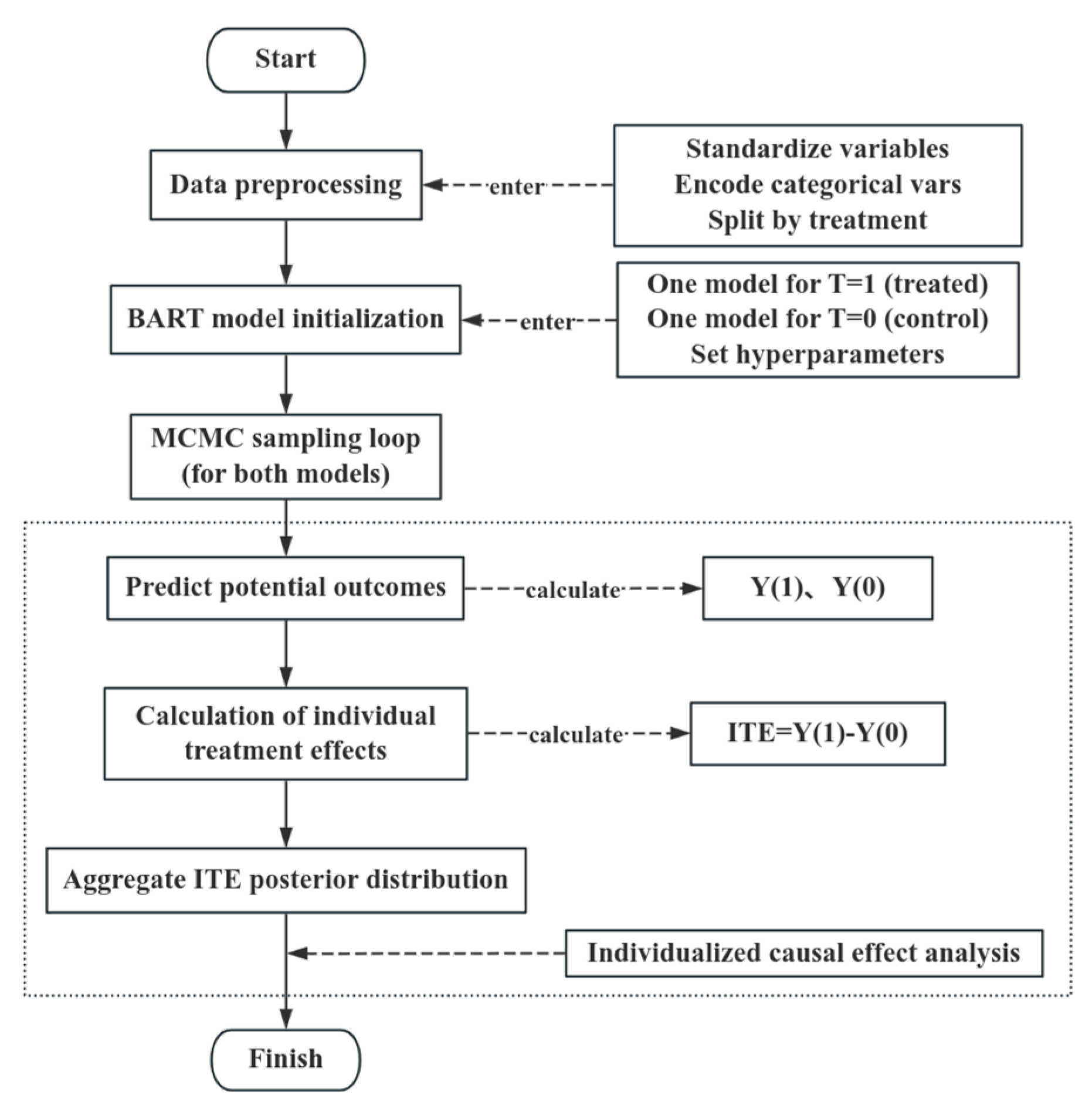
Training phase: Two sets of BART models are trained independently on samples of the treatment group (treatment = 1) and the control group (treatment = 0);

(2)

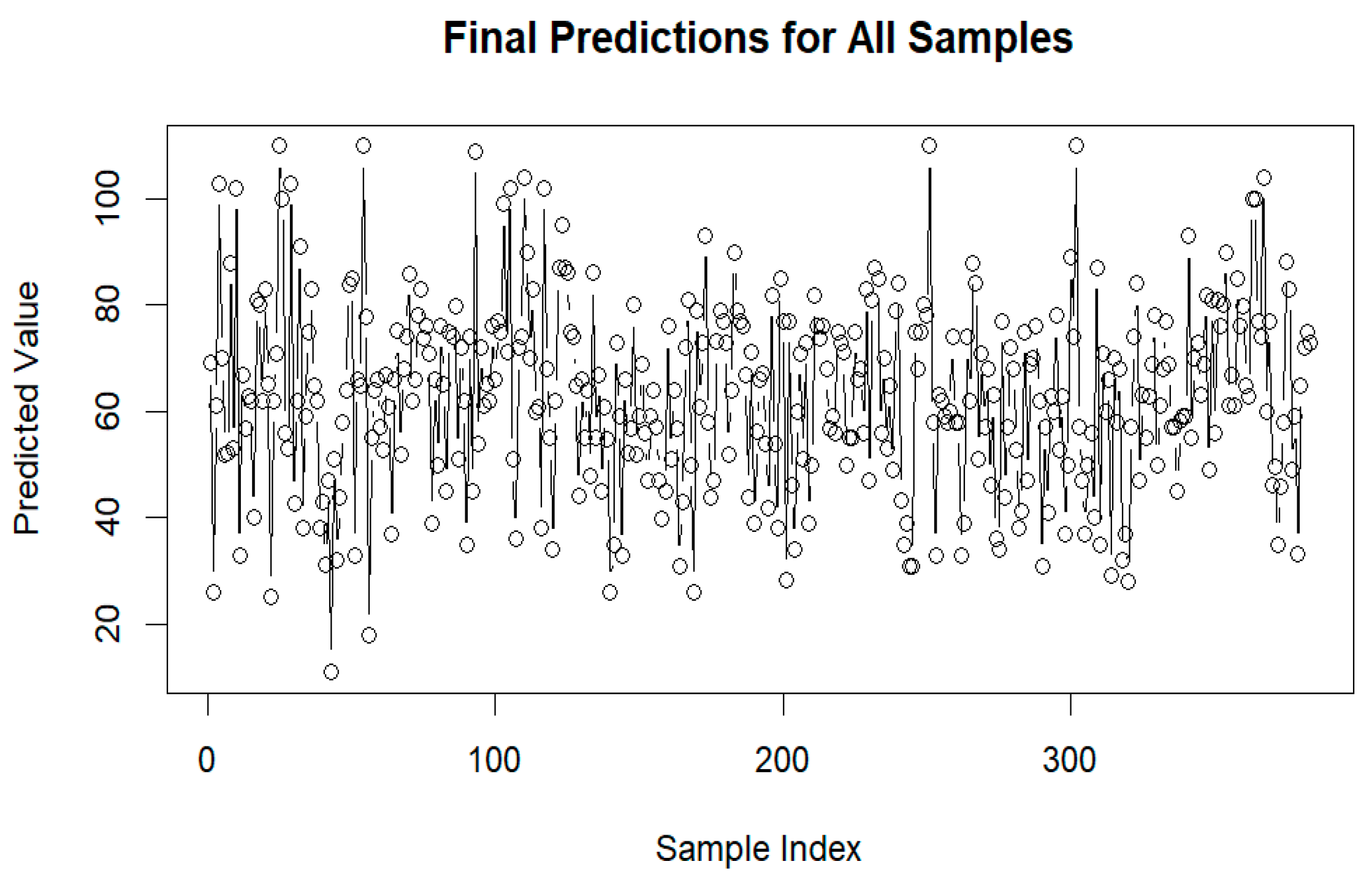
Prediction phase: The two sets of BART models obtained through training are used to predict the potential treatment effects of all observed samples, i.e., the potential results $Y\left(1\right)$ and $Y\left(0\right)$, and calculate the individual ITE.

Therefore, the dual-structure BART-ITE model is computationally equivalent to two complete BART model training and prediction processes. Its overall computational complexity is mainly determined by four core parameters: (a) the number of samples $n$, (b) the number of covariates $p$, (c) the number of trees $m$, (d) the number of MCMC sampling iterations $S$.

During the training phase, the BART model needs to perform tree structure-adjustment operations such as growing, pruning, changing and swapping each tree for each MCMC iteration. The structure adjustment of each tree usually involves traversing a subset of the training data, and the complexity is usually logarithmic with the number of samples, that is, the complexity of a single iteration of each tree is about:

$$O\left(p\times log n\right),$$

where $p$ is the number of covariates, which mainly comes from the need to search for the best splitting variable and splitting point among all covariates when splitting nodes. When the sample size is large or the feature space is complex, especially when $p>50$, $p$ will significantly affect the training time. Since the overall model contains $m$ trees and each MCMC sampling requires $S$ iterations, the overall complexity of the complete training process of a single BART model can be approximately expressed as:

$$O\left(m\times S\times p\times log n\right).$$

For the dual-structure BART-ITE model, two sets of BART models need to be trained independently on the treatment group and the control group, so the total complexity of the training phase is:

$$O\left(2\times m\times S\times p\times log n\right).$$

The number of trees $m$ and the number of MCMC iterations $S$ are the sources of complexity that can be directly controlled when tuning the hyperparameters of the dual-structure BART-ITE model, and a trade-off must be made between computing resources and estimation accuracy.

During the prediction phase, the BART model forward passes the new input data through all trained trees and finally takes the average of the prediction results of all trees. Therefore, the prediction complexity is proportional to the prediction sample size $n_{pred}$ and the number of trees $m$:

$$O\left(m\times n_{pred}\right).$$

The depth of each tree is related to the size of the training data $n$, and the average downstream complexity is $O\left(log n\right)$. For the dual-structure BART-ITE model, two sets of BART models are also needed to predict the potential treatment effects $Y\left(1\right)$ and $Y\left(0\right)$, so the total complexity of the prediction stage is:

$$O\left(2\times m\times n_{pred}\times log n\right).$$

Since the ITE calculation of each sample only involves two simple difference operations of potential results, the computational complexity is $O\left(n_{pred}\right)$, which is negligible compared to the overall complexity of forward propagation, so it is not included in the overall complexity expression separately.

According to the above analysis, the scalability and practicality of the dual-structure BART-ITE model under large-scale datasets can be improved by optimizing the following paths:

(1)

Parallel computing: The tree structure update, MCMC iteration and prediction process in the BART model are highly parallel and can be accelerated by multi-core CPU or GPU. At present, the dbarts package is superior to the classic bartMachine in terms of multi-thread support and memory management, and can significantly improve computing efficiency on medium-sized datasets;

(2)

Efficient software implementation: The dbarts package used in this study has better memory management and parallel efficiency than the classic BART implementation, and can significantly improve the running speed on medium-sized datasets;

(3)

Approximate Bayesian inference: For example, Variational Bayesian BART (VB-BART) can significantly shorten the training time through approximate posterior inference and is suitable for ultra-large-scale data;

(4)

Data subsampling technique: In extremely large-scale scenarios, the BART model can be trained in stages through methods such as data subsampling or local weighted fitting;

(5)

Distributed computing framework: Explore the feasibility of expanding the BART model on a distributed platform, such as combining the Spark + MapReduce framework to implement data segmentation and parallel training of tree models [34], or the BART architecture based on a distributed GPU cluster, which has the potential to further improve the scale and speed of training under ultra-large-scale data.

The dual-structure BART-ITE model has good feasibility and stability on medium-sized datasets; in large-sample high-dimensional feature scenarios, software and hardware collaborative optimization is required to ensure the model’s computational efficiency and estimation accuracy.

4. Simulation Study on the ITE of Graduate Students’ Psychological Stress

4.1. Data Description and Structural Compatibility Test

This study utilized an electronic questionnaire distributed via the “Wenjuanxing” platform (https://www.wjx.cn, accessed on 3 July 2025), which was completed anonymously by respondents. The questionnaire was distributed and collected on 21 November 2024. A total of 420 questionnaires were distributed, and 417 were returned, yielding a high response rate of 99.3%. After screening for invalid responses—such as blank submissions, duplicates or inconsistent entries—34 questionnaires were excluded. Ultimately, 383 valid responses were retained for analysis, representing 91.2% of all distributed questionnaires and 91.8% of the collected ones.

The sample covers multiple universities, offering strong representativeness and analytical value, making it suitable for use in empirical research. All respondents were required to meet the following inclusion criteria:

(i)

Full-time enrollment in a graduate program.

(ii)

A minimum enrollment duration of three months.

(iii)

Clear consciousness and the ability to independently complete the questionnaire.

(iv)

Informed consent was obtained prior to participation.

The questionnaire was carefully designed to reflect the unique characteristics and stress sources of the graduate student population. To control for potential confounding factors, demographic variables such as gender, age, university and academic year were included as covariates. A 10-point Likert scale was employed to assess perceived stress across various domains, where 1 indicates “no stress at all” and 10 represents “extreme stress”.

The questionnaire encompasses 11 specific dimensions: frequency of anxiety, employment pressure, health-related stress, personality-related stress, research-related stress, public social stress, peer social stress, family pressure, advisor-related pressure, financial burden and frequency of self-denial. Individual scores from each dimension were aggregated to compute a total psychological stress score, which serves as a comprehensive measure of each respondent’s overall psychological stress level.

In order to evaluate the structural validity of the questionnaire data in this study, this paper conducted the Kaiser–Meyer–Olkin (KMO) test and Bartlett’s sphericity test on the observed variables. The KMO test is used to measure the common variance between variables. The index ranges from 0 to 1. When the KMO value is greater than 0.80, it is generally believed that the data has good suitability for structural analysis. The Bartlett’s sphericity test is used to test whether the correlation matrix is a unit matrix to evaluate the overall correlation between variables. If the $p$ value is less than 0.05, it indicates that there is a significant correlation between the variables [35]. This paper uses R language to calculate the questionnaire data, and the results are shown in

Table 2. KMO test and Bartlett test.

KMO Test and Bartlett Test
Kaiser–Meyer–Olkin measure of sampling adequacy		0.9010274
Bartlett’s test of sphericity	chisq	2272.322
	p-value	0.000
	df	55

:

The KMO value is 0.9010, indicating that there is a high common variance between the variables; the chi-square statistic of the Bartlett sphericity test is 2272.322, the degrees of freedom is 55 and the corresponding p-value is less than 0.001, rejecting the null hypothesis that “the correlation matrix is the unit matrix”, indicating that the correlation between the variables is significant, confirming that the data in this article meet the prerequisites for subsequent modeling.

4.2. Multivariable Contribution Analysis Based on BART and SHAP

This section uses the processed questionnaire data to construct and train the BART model for 383 individuals in the total sample of graduate students’ psychological stress. The model, implemented in the R language environment (version 4.4.3, released on 28 February 2025), generates 2000 posterior prediction samples, constructs a prediction matrix and calculates the 95% credible interval for each observation. Figure 3 shows the average prediction value of all samples and its corresponding 95% credible interval. The results show that the prediction of the model is generally robust, and the individual differences observed between samples are credible and within a reasonable range, which supports the reliability of the model in capturing uncertainty.

To verify the fitting effect and generalization ability of BART, this paper adopts two methods to evaluate the performance: (a) divide the independent test set for hold-out validation; (b) use 10-fold cross-validation to perform robustness test on the entire sample.

In the independent test, the model performed well on the 30% test samples that did not participate in the training, with a test set $R^2$ of 0.882 and a $RMSE$ of 8.34, indicating that the model has a high prediction accuracy on unseen data. The test set residual distribution is shown in Figure 4 as “Test Set Residuals Distribution”. The center is concentrated and approximately symmetrical, with the peak concentrated near 0, indicating that the BART model has a small prediction deviation and no systematic deviation. The residual range is mainly concentrated within $\pm 20$, further indicating that BART still maintains a low prediction error on unseen data.

In Figure 4, “BART Predictions vs. True Scores” shows the relationship between the predicted values and true values of the BART model on the training set and the test set. Most of the sample points are distributed near the ideal fitting line, especially the training set sample points are highly concentrated, indicating that the model fits the training data well. The test set samples are also closely distributed around the fitting line, without obvious deviation, indicating that the model has good generalization ability.

Subsequently, this study performed 10-fold cross-validation on the BART model and calculated the $R^2$ and $RMSE$ of each fold. Finally, the average and standard deviation were statistically analyzed, as shown in

Table 3. BART model performance under 10-fold cross-validation.

Metric	Mean	SD
$R^2$	0.890	0.061
$RMSE$	8.615	1.820
Overall $R^2$	0.896
Overall $RMSE$	8.773

:

Table 3 shows that the average $R^2$ of 10-fold cross-validation is 0.890, with a standard deviation of 0.061; the average $RMSE$ is 8.615, with a standard deviation of 1.820, indicating that the model’s fitting effect on different subsets is generally stable, and the prediction error fluctuates slightly. To further verify the overall performance of the BART model, this paper also calculates the global performance indicators based on the summary of all prediction results, namely, Overall $R^2$ and Overall $RMSE$, which are 0.896 and 8.773, respectively. The two are basically consistent with the average performance indicators, further proving the consistency and robustness of the model prediction.

In addition, Figure 4 shows the relationship between the predicted value and the true value of each observed sample under 10-fold cross-validation. It can be seen that all prediction points are evenly distributed around the fitting line in the entire score range, indicating that the model has consistent fitting ability in all subsets, without overfitting or underfitting. “10-Fold CV Residuals Distribution” shows the overall distribution of residuals in cross-validation. The residuals show a typical bell-shaped symmetrical distribution with the center concentrated near 0, further indicating that the model prediction error is small overall and the fluctuation is limited.

The $R^2$ of the BART model on the training set is close to 1.0, which may be due to its strong expressive ability. In order to avoid overfitting and falsely high fitting performance, this paper does not use the training set for performance evaluation. All $R^2$ and $RMSE$ indicators are derived from cross-validation and test sets. In addition, the dependent variable is not standardized before modeling, retaining its original explanatory meaning.

To quantify the relative contribution of the 11 characteristic variables, this study applies Shapley value analysis to interpret the output of the BART model. As illustrated in

Table 4. SHAP contribution of each stress factor.

Feature	SHAP Value	Interpretation
Employment Stress ($X_2=9$)	$+$2.4942	The most influential factor significantly increases psychological stress.
Peer Stress ($X_7=3$)	$-$2.3384	Strong negative influence, the strongest protective factor, lower peer pressure reduced psychological distress.
Research Stress ($X_9=8$)	$+$2.0425	Substantial contributor to stress, consistent with academic workload challenges.
Family Stress ($X_8=3$)	$-$1.8182	Lower family stress acts as a buffer, helping reduce overall stress.
Financial Stress ($X_{10}=4$)	$-$1.3256	Suggests moderate financial stress may be less harmful.
Anxiety Frequency ($X_1=8$)	$+$1.3037	Frequent anxiety symptoms are naturally linked to higher psychological stress.
Supervisor Stress ($X_5=8$)	$+$1.1351	The greater pressure from the tutor leads to increased mental tension and stress.
Health Stress ($X_3=6$)	$+$0.5370	Mild health stress contributes only slightly to psychological burden
Social Stress ($X_6=6$)	$-$0.0929	A slightly negative value indicates that social pressure has little impact on the individual.
Negation Frequency ($X_{11}=8$)	$+$0.0673	Negative frequencies play a weaker role.
Personality Stress ($X_4=6$)	$+$0.0231	The effects of personality-related stress were minimal.

and Figure 5, the three most influential factors affecting graduate students’ psychological stress are identified as employment pressure, peer communication pressure and research-related pressure.

Employment pressure exerts the most significant positive impact, among these, with a SHAP value of 2.4942. This indicates that higher levels of stress related to employment substantially increase overall psychological distress. This result aligns with real-world observations, as many graduate students report heightened anxiety and uncertainty regarding their post-graduation career prospects.

Peer communication pressure has a SHAP value of $-2.3384$, making it the most significant negative moderating factor. This suggests that lower levels of peer-related social stress can effectively alleviate psychological distress, while elevated peer pressure may exacerbate mental health issues. The finding underscores the important role of the peer social environment in shaping graduate students’ psychological well-being.

Research pressure, with a SHAP value of 2.0425, is identified as another major positive contributing factor. A heavier research workload is strongly associated with worsening mental health outcomes, likely due to the high intensity, uncertainty, and cognitive demands of academic tasks that characterize the daily lives of graduate students.

In addition, some variables such as family and economic pressure show a certain mitigating effect, while the influence of health, social, emotional and personality pressure is relatively weak.

4.3. Analysis of Group Differences in Employment Stress Among ITE Students

BART is regarded as a “black box” prediction tool, which aims to optimize prediction accuracy rather than establish causal explanations. The SHAP value is mainly used to evaluate the marginal contribution of a certain feature to the prediction result, and its “prediction importance” cannot be automatically converted into the “causal effect” of the variable. However, under the premise of following certain causal inference assumptions, the BART model can serve causal estimation. In Section 4.2, this paper predicts the total score of graduate students’ psychological stress based on the BART model, and uses the SHAP value to evaluate the relative contribution of each variable to the model output. Employment stress shows the strongest predictive importance. The SHAP analysis at this stage is used to identify potential core influencing factors.

In order to explore the heterogeneity of the effect of postgraduate employment stress intervention in different gender and age groups, this paper uses the double-tree BART model to estimate ITE, fitting the potential outcome functions of the high employment stress group and the low employment stress group, respectively. This method, based on the premise assumptions required for causal inference, achieves the estimation of ITE by fully adjusting the covariates and analyzes the impact of the interaction between gender and age on ITE. The study focuses on analyzing the moderating effects of age, gender characteristics and school and gender characteristics on the intervention effect, as shown in Figure 6 and Figure 7. The analysis controls key confounding variables [36].

Figure 6 shows the distribution trend of ITE estimates for graduate students of different genders at different age groups. It can be seen that there is significant heterogeneity in ITE estimates by gender. Gender1 represents female graduate students, and gender2 represents male graduate students. It can be seen from the figure that the estimated ITE values of female graduate students at all ages are generally higher than those of male graduate students, indicating that under the same intervention conditions, the female group benefits more. After the age of 25, the ITE of female graduate students shows a clear upward trend, while the ITE of male graduate students shows a slight decline in some age groups before the age of 25, and only slightly rebounds at around the age of 29, indicating that the responsiveness of the female group to the intervention measures in the employment stress intervention increases with age, while that of the male group is relatively weakened.

The gray shaded area is the uncertainty interval of the model estimation. It can be seen that the credible intervals are wide in the two age groups of 20–22 and 28–30, suggesting that the number of samples in these two age groups is relatively small, and there is a certain uncertainty in the model estimation. The number of samples in these marginal age groups is small, mainly because the natural distribution of the master’s student population in these age ranges is relatively small, and most master’s students are concentrated between 23 and 27 years old. Therefore, this article mainly focuses on the age ranges where the samples are relatively concentrated, and the estimation results of the marginal intervals still need to be further explored in subsequent research based on sample expansion.

To further verify the trend in Figure 6, this study used a multiple linear regression model to analyze the ITE estimates, aiming to test the interactive effect of gender and age. The regression model controlled covariates such as school and grade, and the results are shown in

Table 5. Results of regression analysis of ITE on the interaction between gender and age.

Variable	Estimated Coefficient	p Value	Explain
Intercept	60.5448	<2 × 10−16	Benchmark group ITE (gender1, school1, grade = 0, age = 0)
age	−1.2037	1.45 × 10−13	For every additional year of age, female ITE decreases by about 1.20
gender2	17.4908	0.00207	When the gender is male, the baseline ITE increases by about 17.49
age × gender2	−0.6495	0.00656	For males, ITE decreased by an additional 0.65 for every additional year of age.

:

The regression results show that the coefficient of the interaction term between age and gender is $-0.6495, p=0.00656$, indicating that it is significant at the 1% significance level, that is, there is a significant difference in the age effect of gender in ITE. The ITE of the female group decreases by an average of 1.20 for every 1 year increase in age, while the male group further decreases by 0.65 on this basis, showing a trend that the ITE decreases more significantly with age in males, which is consistent with the trend shown in Figure 6, and further verifies the importance of the interaction between gender and age in ITE estimation from a statistical perspective.

Figure 7 compares the distribution of employment pressure ITEs across four university types and by gender:

(i)

School 1 (non-elite Tier-2 university)—Female students (Gender 1) exhibit slightly higher ITEs than male students (Gender 2). Both genders show modest fluctuations with age. Female ITEs remain relatively stable, with narrow credible intervals, indicating reliable estimates; male ITEs are slightly lower and less sensitive to age.

(ii)

School 2 (non-elite Tier-1 university)—No meaningful gender difference is observed. ITEs for both males and females stay low and flat across ages, with minimal variation. Here, gender and age exert little moderating influence on intervention effects.

(iii)

School 3 (“211” university)—Female students display marginally higher ITEs than males and a gentle upward trend with age. Male ITEs are lower and fairly constant, suggesting that female students respond better to employment-stress interventions, whereas males experience greater baseline stress but weaker gains from the intervention.

(iv)

School 4 (“985” university)—Female students maintain consistently high, stable ITEs with minor age-related variation. By contrast, male students show a pronounced age-related increase: after age 25, their ITEs rise sharply, indicating that employment pressure exerts a growing psychological burden on male postgraduates at top-tier universities.

These patterns highlight the joint moderating roles of institutional prestige and gender: female students generally benefit more from the intervention, whereas male students—especially at highly competitive universities—experience increasing stress and derive less relief as they age.

4.4. Analysis of the Dual-Structure BART-ITE Model

In order to verify the estimation effect of the dual-structure BART-ITE model constructed in this paper on the graduate student psychological stress dataset, this section conducts a systematic analysis from four aspects: (a) model parameter tuning, (b) prediction performance and robustness evaluation, (c) comparative analysis with other causal inference models, (d) operation efficiency evaluation. Through systematic experiments, the comprehensive advantages of the proposed model in terms of accuracy, unbiasedness, generalization ability and scalability are verified.

4.4.1. Hyperparameter Tuning

The BART model itself is non-parametric and flexible, and its performance is greatly affected by hyperparameters in practical applications. Unlike traditional models, BART does not rely on a fixed “number of iterations” as the training termination condition, but instead uses MCMC sampling to estimate the posterior distribution. Therefore, the selection of MCMC sampling parameters—the burn-in period ($nskip$) and the number of effective samples ($ndpost$) is particularly critical. In addition, the model also includes the number of regression trees ($n$), the prior smoothness-control parameter ($k$) and the prior parameter ($\alpha$ and $\beta$) that controls the tree depth. These parameters not only determine the complexity and generalization ability of the model fitting, but also directly affect the accuracy of the ITE estimation. Based on this, this study systematically and phasedly adjusted its key hyperparameters.

In view of the high computational cost caused by the large space of hyperparameter values, this paper divides the parameter-adjustment process into two stages. In the first stage, the grid search method is used to roughly adjust the number of trees and regularization parameters, specifically set to $n\in \left\{50,100,200\right\}$, $k$ from 0.5 to 5.0, with a step size of 0.5; at the same time, the sampling parameters $ndpost=2000$, $nskip=1000$, and the tree depth-control parameters $\alpha =0.95$ and $\beta =2$ are fixed to ensure sampling stability and model convergence. Through this stage, the parameter combination with better performance is selected to lay the foundation for the second stage; in the second stage, based on the optimal number of trees and $k$ value obtained in the first stage, a detailed search is conducted for the tree depth-control parameters $\alpha \in \left\{0.8, 0.9, 0.95, 0.99\right\}$ and $\beta \in \left\{1.5, 2.0, 2.5, 3.0\right\}$ to further improve the smoothness and generalization ability of the model.

During the hyperparameter tuning process, the $RMSE$ and determination coefficient $R^2$ were selected as performance evaluation indicators. The training data and test data were divided in a 7:3 ratio, and the random seed was fixed to ensure the repeatability of the experimental results. Each set of parameters generated prediction results through multiple MCMC sampling, and finally the average of the predicted values was taken to calculate $RMSE$ and $R^2$.

The parameter tuning results of the first stage are shown in Figure 8a. As the k value increases, the $RMSE$ of the model generally shows a downward trend, indicating that the increase in regularization strength helps the model suppress overfitting and improve generalization performance. When $k$ increases from 0.5 to 5.0, the $RMSE$ decreases significantly, especially after $k\ge 3.0$, the downward trend gradually slows down and stabilizes, showing strong robustness. For different numbers of trees, when $n=50$, the $RMSE$ fluctuates greatly and is generally high, and the model performance is unstable, indicating that when the number of trees is insufficient, the model is easily disturbed by data noise and has poor stability. When $n$ increases to 100 and 200, the model error is significantly reduced, the $RMSE$ curve is smoother and more stable overall, and the lowest error level of about 7.6 is reached at $k=5.0$. The performance gap is small, indicating that the marginal benefit of further increasing the number of trees is limited in this dataset. Therefore, based on the comprehensive consideration of model performance and computational cost, $n=100$ and $k=5.0$ are preferred as parameter settings in this paper.

In the first stage, the optimal parameter combination was determined. In the second stage, the tree depth-control parameters $\alpha$ and $\beta$ were further fine-tuned. This paper uses multiple sets of ($n,k,\alpha ,\beta$) parameter combinations for training and calculates the corresponding average $RMSE$. The results are shown in Figure 8b. There are obvious performance differences in $RMSE$ under different parameter combinations.

The best performance was achieved when $n=100$ and $200$, with $RMSE$ generally lower than 8.0, and the top optimal parameter combinations were basically concentrated under these two numbers of trees. When $n=50$, the model stability was poor, and $RMSE$ was significantly higher than other groups, verifying the conclusions drawn in the first stage, that is, under the current data scale, a smaller number of trees is not enough to support the stable convergence of the model. Among all parameter combinations, the best performance is generally concentrated around $\alpha =0.95$ and $\beta =2.0$. Under this combination, the average $RMSE$ of the model can be reduced to about 7.6, achieving the overall optimal performance. When $\beta$ deviates significantly from 2.0 or $\alpha$ is significantly lower than 0.95, the model performance decreases significantly and the $RMSE$ increases to varying degrees, indicating that the tree depth-control parameter has a strong regulatory effect on the model smoothness and fitting ability.

Therefore, considering the performance and stability of the BART-ITE model, the parameter combination in this paper is $n=100$, $k=5.0$, $\alpha =0.95$, $\beta =2.0$. Under this combination, the model can obtain the best fitting effect and generalization performance.

4.4.2. Model Prediction Performance and Robustness Evaluation

Since ITE cannot be directly observed in real data, this paper uses a three-dimensional evaluation system to verify the model performance: (a) estimation accuracy and consistency analysis; (b) effect ranking and heterogeneity structure test; (c) uncertainty-quantification analysis.

Regarding the estimation accuracy and consistency analysis of the dual-structure BART-ITE model, the model is tested using three methods: Bootstrap sampling, cross-validation and sensitivity analysis. The results are shown in

Table 6. Results of different evaluation methods for the dual-structure BART-ITE model.

Verification Method	RMSE	Bias
Bootstrap	10.71	23.15
Cross-validation	7.67	-
Pseudo-ITE comparison by matching method	21.77	$-$1.72

:

The Bootstrap method evaluates the stability of the model on different samples through multiple resampling, which can effectively avoid the deviation caused by data division. Its evaluation results show that under multiple resampling, the $RMSE$ of the model is 10.71 and the Bias is 23.15, indicating that the model in this paper has good stability under different resampling samples.

The cross-validation method divides the data into multiple folds, trains and tests each fold, and can reflect the generalization ability of the model under different data divisions. The evaluation results of cross-validation show that the model performs well on different folds, with an $RMSE$ of 7.67, showing that the generalization ability of the model is superior to that of the Bootstrap method.

Sensitivity analysis compares the estimation results of the dual-structure BART-ITE model with the pseudo-ITE. In the comparison with the pseudo-ITE, the $RMSE$ of the model is 21.77 and the Bias is $-$1.72, indicating that the model estimation results are highly consistent with the pseudo-ITE and the error is within a reasonable range, which further enhances the reliability of the model.

In addition to error assessment, the dual-structure BART-ITE model is also very important for identifying and ranking effect heterogeneity. Figure 9 shows the performance of the model from three dimensions:

Figure 9A is the uplift curve, which rises rapidly in the first part and then stabilizes, indicating that the model has good sorting ability in identifying high ITE subgroups. The corresponding AUUC value is 133.389, indicating that the model has significant advantages in distinguishing individuals with high and low treatment effects.

Figure 9B shows the relationship between the 95% credible interval width and the predicted ITE value. The curve shows a typical U-shaped trend, indicating that the model has a narrower credible interval at the medium effect level, that is, a higher estimation stability, and a wider uncertainty interval in the low and high effect areas, which reflects that the model performs reasonably in balancing the reliability of estimation and risk control. The average value of the credible interval width is 36.163, and the range of the predicted ITE value is 45.824, which further shows that the model can better balance the reliability of estimation and risk control when dealing with individuals with different effect levels.

Figure 9C shows the distribution of the model-predicted ITE values, which show overall discreteness and a multi-peak structure, reflecting the strong heterogeneity of treatment effects among individuals. The red dashed line in the figure indicates the average predicted ITE value, which equals the model output value of 22.56, further supporting the model’s ability to effectively depict individual differences.

Regarding the ability of the dual-structure BART-ITE model to identify the effect heterogeneity structure, this study used the Grouped Average Treatment Effect (GATE) method to divide the test set samples into five quantile groups according to the predicted ITE. The average ITE of each group was 11.3, 19.9, 23.7, 27.6 and 33.3, respectively, showing an obvious monotonically increasing trend, indicating that the model can distinguish individuals with different effect levels. The further one-way ANOVA result was $F=175.1, p<0.001$, and the difference between the groups was significant, which verified the effectiveness of the model in identifying the heterogeneity of effects between individuals.

Due to the lack of real ITE labels, some indicators that rely on real counterfactuals, such as PEHE (Precision in Estimation of Heterogeneous Effect) and coverage, cannot be used in this study; at the same time, since the observational data cannot construct an ideal double randomized experimental environment, the use of some verification indicators is also limited. Therefore, this paper combines the current research conditions and constructs a multivariate evaluation system to systematically evaluate the comprehensive performance of the dual-structure BART-ITE model in actual application scenarios from four dimensions: error analysis, heterogeneity identification, sorting ability and uncertainty quantification.

4.4.3. Comparative Analysis with Other ITE-Estimation Models

In order to systematically evaluate the performance of the proposed dual-structure BART-ITE model, the paper first compares the dual-structure BART-ITE model with the common single-tree structure BART model, as shown in Figure 10a.

Figure 10a is the ITE-estimation distribution histogram of the dual-structure BART-ITE model and the single-tree structure BART model on the training set. It can be seen that the ITE values estimated by the single-tree model are mainly concentrated in the $[15, 25]$ interval, with a relatively concentrated distribution pattern and a relatively low mean. The ITE distribution of the dual-structure structure is more dispersed, with obvious long-tail characteristics, especially in the ITE > 30 region, indicating that it has a stronger ability to express individual heterogeneity. At the same time, the mean under the dual-structure structure is slightly higher than that of the single-tree structure, indicating that its estimated overall treatment effect is stronger.

Furthermore, this paper selects the current mainstream ITE-estimation methods as comparison benchmarks, including X-Learner, S-Learner, T-Learner, BCF and linear models. The comparison indicators include $RMSE$, Bias and CI Width, which measure the performance of the model in terms of accuracy, unbiasedness and uncertainty control, respectively.

The results are shown in Figure 10b. The dual-structure BART-ITE model performs well in both $RMSE$ and credible interval width, which are 19.76 and 28.68, respectively, significantly better than other models, indicating that it has significant advantages in estimation accuracy and credibility control. Although X-Learner is close to it in $RMSE$, its credible interval is slightly wider, indicating that the uncertainty of its estimation results is slightly higher.

In contrast, S-Learner and T-Learner have certain deficiencies in bias control, which are $-$12.08 and $-$14.02, respectively, and the corresponding CI widths are also large, reflecting that the model estimation has certain volatility. BCF and linear models are relatively stable in bias control, but their $RMSE$ and interval widths are generally large, especially the CI width of BCF is as high as 42.34, indicating that its estimation of individual effects is less reliable.

Based on the above analysis, the dual-structure BART-ITE model achieves a good balance between accuracy, unbiasedness and uncertainty, verifying its effectiveness and applicability in the task of modeling individual causal effects.

4.4.4. Operational Efficiency and Computing Resource Evaluation

Section 3.4 discussed the complexity and scalability of the dual-structure BART-ITE model. This section evaluates the operating efficiency of the dual-structure BART-ITE model under different parameter settings based on empirical data, analyzes the sensitivity of training time to changes in sample capacity, number of trees and number of MCMC iterations, and discusses its feasibility in large-scale data applications.

The specific experimental design of this study is to select the training samples in the dataset in Section 4.1 and test the training time of the dual-structure BART-ITE model under the following parameter combinations:

(a)

Sample size $n$: 100, 200 and 342;

(b)

Number of trees $m$: 50, 100 and 200;

(c)

MCMC iteration number $S$: 1000 and 2000, with burn-in set to 0.5$S$.

Under each set of parameter combinations, two dbarts models, the treatment group and the control group, were trained, respectively, and the total time/second spent on training was recorded. The entire process was run in a single-core CPU environment without enabling parallel acceleration.

From

Table 7. Training time of the dual-structure BART-ITE model with different parameter combinations.

n	m	S	Training Time (Seconds)
100	50	1000	0.27
100	50	2000	0.47
100	100	1000	0.47
100	100	2000	0.93
100	200	1000	0.92
100	200	2000	1.77
200	50	1000	0.28
200	50	2000	0.51
200	100	1000	0.50
200	100	2000	1.00
200	200	1000	0.98
200	200	2000	1.94
342	50	1000	0.30
342	50	2000	1.09
342	100	1000	0.59
342	100	2000	1.14
342	200	1000	1.11
342	200	2000	2.23

, we can conclude that:

(1)

The model training time increases approximately linearly with the number of trees $m$ and the number of MCMC iterations $S$;

(2)

When the sample size n increases, the training time also increases, but the increase is relatively mild, mainly due to the good processing efficiency of dbarts for sample size;

(3)

Under the maximum setting of $n=342, m=200, S=2000,$ the training time is about 2.23 s, which is generally controllable.

To further show the growth trend of training time, a line graph and a heat map of training time changing with parameters are drawn, as shown in Figure 11a,b.

From the line graph Figure 11a, we can see that under a fixed sample size, the training time increases with the increase in $m$ and $S$, and presents a stable linear relationship, indicating that the number of trees and the number of iterations are the core factors affecting the computational complexity of BART, which is consistent with the theoretical complexity $O\left(nmS\right)$ expectation. The heat map Figure 11b further shows that under actual small sample data, even with a higher model complexity setting, a single training only takes $1~2$ s, which can meet the current experimental needs.

4.5. Local Interpretation of ITE Based on SHAP

The importance of global variables in Section 4.2 shows that employment pressure is the most important factor affecting the psychological stress of graduate students. Section 4.3 further explores the heterogeneous characteristics of the group. This section combines SHAP to perform local feature contribution decomposition on the individual ITE values estimated by the double-tree BART-ITE model, quantifying the specific contribution of each covariate to the individual ITE value, aiming to reveal why the model produces a high or low ITE value for a specific individual, and strengthen the explanation of the association between global variable importance and individual prediction mechanism.

This paper uses the Shapley module under the iml package in the R language environment (version 4.4.3, released on 28 February 2025) to perform individual prediction decomposition on the results obtained from the training of the double-tree BART-ITE model for the treatment group and the control group. Taking the first sample in the training set as an example, its basic features are $\mathrm{g}\mathrm{e}\mathrm{n}\mathrm{d}\mathrm{e}\mathrm{r}=1, \mathrm{a}\mathrm{g}\mathrm{e}=25,\mathrm{g}\mathrm{r}\mathrm{a}\mathrm{d}\mathrm{e}=2, \mathrm{s}\mathrm{c}\mathrm{h}\mathrm{o}\mathrm{o}\mathrm{l}=3$, corresponding to a 25-year-old male second-year graduate student from a 211 university.

Table 8. SHAP value decomposition results of the first sample in the treatment group and the control group.

Group	Feature	SHAP Value (ϕ)	Contribution Variance (ϕ.var)	Feature Value
Treated	gender	0.390	0.412	gender = 1
	age	0.026	2.938	age = 25
	grade	$-$1.120	1.050	grade = 2
	school	$-$2.717	7.296	school = 3
Control	grade	3.086	9.228	grade = 2
	school	1.391	3.671	school = 3
	gender	1.010	2.852	gender = 1
	age	$-$1.038	20.668	age = 25

and Figure 12 show the SHAP local explanation results of this individual in two scenarios.

In the treated group, the school feature $\varphi =-2.717$ has the most significant negative contribution to the prediction results, followed by the grade feature $\varphi =1.120$, while the marginal contributions of gender and age are relatively small, $\varphi =0.390$ and $\varphi =0.026$, showing a slight positive effect. This shows that in the scenario of employment stress intervention, the school category and grade of the individual are the main factors affecting the space for reducing their stress scores.

In the control group, the grade feature $\varphi =3.086$ has the strongest positive contribution, followed by school and gender, $\varphi =1.391$ and $\varphi =1.010$, while age has a certain negative impact, $\varphi =-1.038$. It can be seen that when no intervention is received, grade and school background dominate the formation mechanism of stress scores.

The above ITE local interpretation results show that even under the same individual characteristics, the dual-structure BART-ITE model has obvious differences in the prediction contribution mechanism for different treatment scenarios. The marginal contribution direction and intensity of school type and grade in the treatment group and the control group have changed significantly, which reflects the potential mechanism of the intervention policy to produce heterogeneous effects in student groups with different academic backgrounds. Multiple individuals were randomly selected from the sample set and the same SHAP local decomposition analysis was performed. The grade, school category and gender variables showed highly stable importance characteristics in the ITE formation mechanism of most samples, but there were still certain individual differences in the specific contribution direction and intensity, which reflected the effectiveness of the dual-structure BART-ITE model in capturing the heterogeneity of individualized treatment effects.

5. Conclusions

This study focuses on the problem of accurate estimation of ITEs and proposes a dual-structure causal inference model based on BART, namely BART-ITE. This model constructs a dual BART structure of the treatment group and the control group, and uses the MCMC method to perform posterior sampling of potential results to achieve the estimation of causal effects at the individual level. Through an empirical study of graduate students’ psychological stress questionnaire data, it is found that employment stress is the core factor affecting psychological state. On this basis, its individualized intervention effect is estimated, further verifying the advantages of the dual-structure BART-ITE in improving the accuracy of causal inference.

The BART-ITE model has the potential to expand in many directions:

(1)

Dynamic causal inference: With the growing availability of multimodal and time-series data, the dual-structure BART-ITE model can be extended to estimate time-varying treatment effects and incorporate temporal dependencies [37].

(2)

Integration with deep learning: By embedding the dual-structure BART-ITE model within deep learning architectures and incorporating automatic feature extraction, the framework can be further adapted to handle nonlinear, highly complex structures [38].

(3)

In terms of real-world applications, the dual-structure BART-ITE offers substantial value in domains such as precision medicine, policy evaluation and educational resource optimization. Future work may explore integrating the model with online learning algorithms to support real-time updates and adaptive causal analysis, thereby enhancing its responsiveness and practical utility in dynamic environments.

References

1. Li, T.; Guan, J.; Huang, Y.; Jin, X. The Effect of Stress on Depression in Postgraduate Students: Mediating Role of Research Self-Efficacy and Moderating Role of Growth Mindset. Behav. Sci. 2025, 15, 266. [Google Scholar] [CrossRef]
2. Soma, S.; Dipanjan, B.; Prasad, K.; Hariom, P.; Sourav, K. A Comparison of Stress, Coping, Empathy, and Personality Factors Among Post-Graduate Students of Behavioural Science and Engineering Courses. Indian J. Psychiatry 2023, 65, 113–114. [Google Scholar] [CrossRef]
3. Prout, T.A.; Zilcha-Mano, S.; Aafjes-van Doorn, K.; Békés, V.; Christman-Cohen, I.; Whistler, K.; Kui, T.; Di Giuseppe, M. Identifying Predictors of Psychological Distress During COVID-19: A Machine Learning Approach. Front. Psychol. 2020, 11, 586202. [Google Scholar] [CrossRef] [PubMed]
4. Adhikari, S.; Zheleva, E. Inferring Individual Direct Causal Effects under Heterogeneous Peer Influence. Mach. Learn. 2025, 114, 113. [Google Scholar] [CrossRef]
5. Samuel, B.; Matias, B.; Michele, G. Helping Struggling Students and Benefiting All: Peer Effects in Primary Education. J. Public Econ. 2023, 224, 104925. [Google Scholar] [CrossRef]
6. Xiao, Z.M.; Hauser, O.P.; Kirkwood, C.; Li, D.Z.; Jones, B.; Higgins, S. Uncovering Individualised Treatment Effect: Evidence from Educational Trials. OSF Preprints, 2020; preprint. [Google Scholar] [CrossRef]
7. Xiang, Z.; Xie, Y. Propensity Score-Based Methods versus MTE-Based Methods in Causal Inference: Identification, Estimation, and Application. Sociol. Methods Res. 2016, 45, 3. [Google Scholar]
8. Hettinger, G.; Lee, Y.; Mitra, N. Multiply robust difference-in-differences estimation of causal effect curves for continuous exposures. Biometrics 2025, 81, ujaf015. [Google Scholar] [CrossRef]
9. Liu, Z.; Sun, Y.; Li, Y.; Li, Y. Doubly robust estimation for non-probability samples with heterogeneity. J. Comput. Appl. Math. 2025, 465, 116567. [Google Scholar] [CrossRef]
10. Mullainathan, S.; Spiess, J. Machine learning: An applied econometric approach. J. Econ. Perspect. 2017, 31, 87–106. [Google Scholar] [CrossRef]
11. He, W.J.; You, D.F.; Zhang, R.Y.; Yu, H.; Chen, F.; Hu, Z.B.; Zhao, Y. Estimation on the Individual Treatment Effect among Heterogeneous Population, Using the Causal Forests Method. Zhonghua Liu Xing Bing Xue Za Zhi 2019, 40, 707–712. [Google Scholar] [CrossRef]
12. Goedhart, M.J.; Klausch, T.; Janssen, J.; van de Wiel, M.A. Adaptive Use of Co-Data Through Empirical Bayes for Bayesian Additive Regression Trees. Stat. Med. 2025, 44, e70004. [Google Scholar] [CrossRef]
13. Sparapani, R.A.; Logan, B.R.; McCulloch, R.E.; Laud, P.W. Nonparametric Survival Analysis Using Bayesian Additive Regression Trees (BART). Stat. Med. 2016, 35, 2741–2753. [Google Scholar] [CrossRef] [PubMed]
14. Chipman, H.A.; George, E.I.; McCulloch, R.E. BART: Bayesian Additive Regression Trees. Ann. Appl. Stat. 2010, 4, 266–298. [Google Scholar] [CrossRef]
15. Zhao, Y.; Liu, R.; Lin, J.; Chi, A.; Davies, S. DOD-BART: Machine Learning-Based Dose Optimization Design Incorporating Patient-Level Prognostic Factors via Bayesian Additive Regression Trees. J. Biopharm. Stat. 2024, 34, 11–16. [Google Scholar] [CrossRef]
16. Lewis, M.; Liu, Y.; Goyal, N.; Ghazvininejad, M.; Mohamed, A.; Levy, O.; Stoyanov, V.; Zettlemoyer, L. BART: Denoising Sequence-to-Sequence Pre-Training for Natural Language Generation, Translation, and Comprehension. arXiv 2019, arXiv:1910.13461. [Google Scholar]
17. Rossouw, R.F.; Coetzer, R.L.J.; Le Roux, N.J. Variable Contribution Identification and Visualization in Multivariate Statistical Process Monitoring. Chemom. Intell. Lab. Syst. 2020, 196, 103894. [Google Scholar] [CrossRef]
18. Del Serrone, G.; Moretti, L. A Stepwise Regression to Identify Relevant Variables Affecting the Environmental Impacts of Clinker Production. J. Clean. Prod. 2023, 398, 136564. [Google Scholar] [CrossRef]
19. Dubey, A.K.; Kumar, Y.; Kumar, S. Optimizing Parameters of AWJM for Ti-6Al-4V Grade 5 Alloy Using Grey Entropy Weight Method: A Multivariable Approach. J. Inst. Eng. Ser. C 2025, 106, 181–195. [Google Scholar] [CrossRef]
20. Lundberg, S.; Lee, S.I. A Unified Approach to Interpreting Model Predictions. arXiv 2017. [Google Scholar] [CrossRef]
21. Akter, R.; Susilawati, S.; Zubair, H.; Chor, W.T. Analyzing Feature Importance for Older Pedestrian Crash Severity: A Comparative Study of DNN Models, Emphasizing Road and Vehicle Types with SHAP Interpretation. Multimodal Transp. 2025, 4, 100203. [Google Scholar] [CrossRef]
22. Ji, Y.; Shang, H.; Yi, J.; Zang, W.; Cao, W. Machine Learning-Based Models to Predict Type 2 Diabetes Combined with Coronary Heart Disease and Feature Analysis Based on Interpretable SHAP. Acta Diabetol. 2025, 62, 1–16. [Google Scholar] [CrossRef] [PubMed]
23. Neubauer, A.; Brandt, S.; Kriegel, M. Explainable Multi-Step Heating Load Forecasting: Using SHAP Values and Temporal Attention Mechanisms for Enhanced Interpretability. Energy AI 2025, 14, 100480. [Google Scholar] [CrossRef]
24. Aman, N.; Panyametheekul, S.; Pawarmart, I.; Sudhibrabha, S.; Manomaiphiboon, K. A Visibility-Based Historical PM2.5 Estimation for Four Decades (1981–2022) Using Machine Learning in Thailand: Trends, Meteorological Normalization, and Influencing Factors Using SHAP Analysis. Aerosol Air Qual. Res. 2025, 25, 4. [Google Scholar] [CrossRef]
25. Yu, L.; Jian, W.; Bing, L. EDVAE: Disentangled Latent Factors Models in Counterfactual Reasoning for Individual Treatment Effects Estimation. Inf. Sci. 2024, 652, 119578. [Google Scholar] [CrossRef]
26. Marchezini, G.F.; Lacerda, A.M.; Pappa, G.L.; Meira, W.; Miranda, D.; Romano Silva, M.A.; Diniz, L.M. Counterfactual inference with latent variable and its application in mental health care. Data Min. Knowl. Discov. 2022, 36, 811–840. [Google Scholar] [CrossRef]
27. Winship, C.; Morgan, S.L. The estimation of causal effects from observational data = L’évaluation des effets de causalité à partir de données d’observation. Annu. Rev. Sociol. 1999, 25, 659–706. [Google Scholar] [CrossRef]
28. Hill, J.L. Bayesian nonparametric modeling for causal inference. J. Comput. Graph. Stat. 2011, 20, 217–240. [Google Scholar] [CrossRef]
29. Carone, M.; Bignozzi, G.; Manolopoulou, I. Shrinkage Bayesian causal forests for heterogeneous treatment effects estimation. J. Comput. Graph. Stat. 2022, 31, 1202–1214. [Google Scholar] [CrossRef]
30. Kalu, C.; Stephen, B.U.A.; Uko, M.C. Empirical valuation of multi-parameters and RMSE-based tuning approaches for the basic and extended Stanford University Interim (SUI) propagation models. Math. Softw. Eng. 2017, 3, 1–12. [Google Scholar]
31. Macedo, F.L.; Reverter, A.; Legarra, A. Behavior of the linear regression method to estimate bias and accuracies with correct and incorrect genetic evaluation models. J. Dairy Sci. 2020, 103, 529–544. [Google Scholar] [CrossRef]
32. Marvald, J.; Love, T. Detecting interactions using Bayesian additive regression trees. Pattern Anal. Appl. 2024, 27, 153. [Google Scholar] [CrossRef]
33. Ročková, V.; van der Pas, S. Posterior concentration for Bayesian regression trees and forests. Ann. Stat. 2020, 48, 2108–2131. [Google Scholar] [CrossRef]
34. Guo, Y.; Zhang, Z.; Jiang, J.; Wu, W.; Zhang, C.; Cui, B.; Li, J. Model averaging in distributed machine learning: A case study with Apache Spark. VLDB J. 2021, 30, 693–712. [Google Scholar] [CrossRef]
35. Liu, Z.; Yuan, F.; Zhao, J.; Du, J. Reliability and validity of the positive mental health literacy scale in Chinese adolescents. Front. Psychol. 2023, 14, 1150293. [Google Scholar] [CrossRef]
36. Mirhaghi, A.; Sittichanbuncha, S. Observer heterogeneity can be thought of as a confounding variable. Asian Biomed. 2016, 10, 393. [Google Scholar] [CrossRef]
37. Papaspyropoulos, K.G.; Kugiumtzis, D. On the validity of Granger causality for ecological count time series. Econometrics 2024, 12, 13. [Google Scholar] [CrossRef]
38. He, R.; Liu, M.; Lin, Z.; Zhuang, Z.; Shen, X.; Pan, W. DeLIVR: A deep learning approach to IV regression for testing nonlinear causal effects in transcriptome-wide association studies. Biostatistics 2023, 25, 468–485. [Google Scholar] [CrossRef]
Figure 1. Main algorithm flow chart.
Mathematics 13 02195 g001
Figure 2. Sub-flowchart of the MCMC sampling loop.
Mathematics 13 02195 g002
Figure 3. Final predicted values for 383 samples and their corresponding credible intervals.
Mathematics 13 02195 g003
Figure 4. Visualization of BART model performance and residual analysis.
Mathematics 13 02195 g004
Figure 5. Multivariate SHAP value contribution plot.
Mathematics 13 02195 g005
Figure 6. Employment pressure distribution of ITE by age and gender.
Mathematics 13 02195 g006
Figure 7. Distribution of employment pressure in ITE by school and gender.
Mathematics 13 02195 g007
Figure 8. Two-stage parameter sensitivity and performance analysis. (a) The first stage parameter sensitivity analysis diagram; (b) Performance analysis of the second stage parameter combination.
Mathematics 13 02195 g008
Figure 9. ITE-estimation performance visualization using BART-ITE. (A) Uplift curve with the AUUC value. (B) Relationship between 95% CI width and predicted ITE. (C) Distribution of predicted ITE values.
Mathematics 13 02195 g009
Figure 10. Comparative analysis of the dual-structure BART-ITE model. (a) ITE-estimation distribution histogram of the dual-structure BART-ITE model and the single-tree structure BART-ITE model on the training set (the blue columns represent the single-tree structure, the red columns represent the dual-structure, the red and blue dashed lines represent the average ITE values of the dual-structure model and the single-structure model, respectively. (b) Performance comparison of different ITE estimation methods in terms of RMSE, Bias and CI Width.
Mathematics 13 02195 g010
Figure 11. Parameter-specific training time analysis of the dual-structure BART-ITE model. (a) Line graph of training time versus number of trees and iterations. (b) Heat map of training time under different parameter settings.
Mathematics 13 02195 g011
Figure 12. SHAP explanation diagram at local individual level.
Mathematics 13 02195 g012