Abstract
Accurate wind power forecasting is critical for grid management and low-carbon transitions, yet challenges arise from wind dynamics’ nonlinearity and randomness. Existing methods face issues like suboptimal hyperparameters and a poor spatiotemporal feature integration. This study proposes OPESC-CNN-BiLSTM-SA, a hybrid model combining an optimized escape algorithm (OPESC), convolutional neural network (CNN), bidirectional long short-term memory (BiLSTM) network, and self-attention (SA). The OPESC tunes critical hyperparameters, including the learning rate, the number of BiLSTM hidden units, self-attention key/query dimensions, and the L2 regularization strength, to enhance model generalization. Meanwhile, the CNN extracts spatial features, the BiLSTM captures bidirectional temporal dependencies, and SA dynamically weights critical features. Testing on real wind farm data shows the model reduces the RMSE by 30.07% and the MAE by 34.51%, and achieves an R2 of 97.06% compared to the baseline, demonstrating an improved accuracy for non-stationary energy time series forecasting.
Keywords:
wind power forecasting; escape algorithm (ESC); convolutional neural network (CNN); bidirectional long short-term memory network (BiLSTM); self-attention mechanism MSC:
68T07
1. Introduction
Since the turn of the 21st century, the global energy transition has accelerated, with wind power garnering an extensive adoption due to its environmentally friendly and low-carbon attributes [1]. However, wind power generation is influenced by multiple factors, such as the wind speed and temperature, exhibiting significant nonlinearity, non-stationarity, and randomness. Specifically, the pronounced nonlinearity implies that the relationship between meteorological inputs and the power output cannot be adequately captured by traditional linear frameworks, as minor perturbations in boundary conditions can induce disproportionately large fluctuations in the generation [2]. Non-stationarity stems from the time-varying statistical properties of meteorological signals—such as seasonal cycles, diurnal fluctuations, and abrupt climate anomalies—which invalidate the stationary assumptions of traditional time series methods like ARIMA [3]. Meanwhile, randomness originates from chaotic micro-scale meteorological phenomena and measurement uncertainties, introducing irreducible noise that complicates the pattern extraction [4]. Consequently, these characteristics pose substantial challenges for achieving a high forecast accuracy. The precision of these predictions directly affects the grid dispatch, energy storage optimization, and market stability, while also playing a crucial role in enhancing the wind farm operational efficiency and reducing energy costs [5,6,7]. Therefore, developing accurate wind power forecasting models is essential for providing a theoretical basis for the grid power balance and renewable energy integration planning, thereby promoting the green, low-carbon energy transition [8,9].
Current methods for wind power forecasting can be categorized into three main types: physical methods [10], statistical methods [11], and artificial intelligence methods [12]. Physical approaches rely on numerical weather prediction (NWP) models to simulate meteorological parameters, such as the wind speed and direction, using atmospheric dynamic equations and then estimate the wind power output [13]. For instance, Al-Yahyai et al. [14] reviewed the application of NWP models in wind energy assessments, highlighting their ability to overcome the low resolution and site limitations of traditional meteorological station data, making them suitable for mid-to-long-term forecasting. However, the high computational complexity of NWP models and their limited capacity to resolve micro-scale phenomena fundamentally constrain their ability to capture transient fluctuations and nonlinear responses in wind power generation, resulting in a suboptimal accuracy and practicality for high-value short-term forecasting scenarios [15]. Statistical methods, on the other hand, construct linear forecasting models—such as autoregressive moving averages (ARMAs) and seasonal ARIMAs (SARIMAs)—by leveraging the time series characteristics of historical data. The models are relatively simple, computationally efficient, and perform well on stationary time series data [16]. For instance, Wang et al. [17] applied the ARMA model for short-term wind power prediction, effectively reducing forecasting errors; however, the method’s reliance on the assumption of data stationarity makes it less capable of handling nonlinear issues, such as abrupt wind speed changes [18]. Traditional statistical models exhibit limited adaptability to evolving data distributions under nonlinear effects caused by abrupt wind variations, extreme weather, or a complex topography, resulting in substantially increased prediction errors and a diminished robustness.
In recent years, artificial intelligence techniques have significantly improved the modeling of nonlinear relationships by utilizing machine learning and deep learning methods, surpassing the limitations inherent in physical and statistical approaches. For example, Guo et al. [19] employed a BP neural network to integrate multi-source meteorological data, achieving a 24 h wind power prediction accuracy of 85.6%. With the advancement of deep learning, long short-term memory (LSTM) networks and their variants have become prevalent. Shahid et al. [20] introduced a GA-optimized LSTM (GLSTM) network that adaptively adjusts hyperparameters, reducing prediction errors by 6–30% compared to conventional LSTM models. Additionally, convolutional neural networks (CNNs) have shown a remarkable performance in spatial feature extraction; Zhu et al. [21] demonstrated the feasibility of CNNs in wind power regression. However, single models exhibit inherent limitations in complex scenarios, such as LSTM struggling to capture spatial features and the CNN failing to efficiently model long-term temporal dependencies. To address this, research has progressively shifted toward multi-model fusion strategies. For example, Chen et al. [22] combined a CNN with bidirectional LSTM (BiLSTM) and employed a feature weighting strategy, remarkably enhancing the time series data utilization and forecasting accuracy. Further advancements include Zhang et al. [23], who proposed a multi-task learning model integrating a Transformer and LSTM, leveraging dilated causal convolutional networks to extract multi-dimensional features for both deterministic and probabilistic wind power forecasting—reducing the Mean Absolute Error by up to 9.190 compared to 23 benchmark models. Additionally, Zhao et al. [24] developed a hybrid VMD-CNN-GRU framework, where the variable mode decomposition preprocesses wind speed sequences to mitigate volatility, and a CNN collaborates with a GRU to extract spatial–temporal features, achieving an RMSE of 1.5651 and an R2 of 0.9964 in short-term predictions. These studies highlight that multi-model architectures overcome single-model constraints and enhance the prediction performance in complex energy systems through approaches such as structural integration, task-sharing, or data decomposition.
The performance of these models largely depends on the selection of hyperparameters, making hyperparameter optimization a critical step in enhancing prediction accuracy [25]. The full realization of a model’s potential is critically constrained by whether its hyperparameters are optimally configured. Inappropriate hyperparameters can directly lead to model underfitting or overfitting, even if the model itself possesses strong capabilities. Traditional methods such as the grid search and random search, although simple and easy to implement, suffer from significant efficiency drops when dealing with high-dimensional parameter spaces and complex models [26]. For example, deep neural networks, such as LSTM and CNN, often contain dozens of hyperparameters. Traditional methods face the problem of exponential growth in computational complexity with the increase in dimensions [27], which leads to an exponential increase in the computational cost and an extremely low efficiency. As a result, traditional methods usually can only carry out a rough exploration within a limited range, making it difficult to find the global or near-global optimal solution. Consequently, intelligent optimization algorithms have gradually become the mainstream approach, balancing the global search and local exploitation by simulating natural evolution or swarm intelligence. Shahid et al. [20] utilized a genetic algorithm (GA) in their GLSTM model to optimize both the time window length and the number of hidden neurons, achieving a 6–30% reduction in forecasting errors across multiple scenarios in seven major European wind farms. Furthermore, Geng et al. [28] developed a hybrid PSO–deep reinforcement learning (DRL) framework that combines Particle Swarm Optimization with deep reinforcement learning, reducing the system’s Mean Squared Error (MSE) by 23.8%. Gao et al. [29] used the sparrow search algorithm (SSA) to adaptively optimize the variational mode decomposition (VMD), significantly enhancing LSTM’s short-term prediction accuracy; Lu et al. [30] employed gray wolf optimization (GWO) to simultaneously optimize the kernel parameters of a multi-output support vector machine (MSVM), outperforming single-model forecasting frameworks; Li et al. [31] compared an improved dragonfly algorithm with traditional strategies, demonstrating that the former could more efficiently search the SVM hyperparameter space, resulting in a 23.6% reduction in forecasting errors on French wind farm data compared to BP neural networks; similarly, in regional load forecasting, Barman et al. [32] showed that an SVM model optimized by the grasshopper optimization algorithm (GOA), which incorporates an analysis of similar climate days, improved the prediction accuracy by 12.6% and 8.3% relative to the GA-SVM and PSO-SVM, respectively. Although intelligent optimization algorithms can enhance the efficiency and effectiveness of the hyperparameter search, they still have significant defects. Concerning local optimality and convergence, the genetic algorithm (GA) tends to be trapped in local optima when handling multimodal functions [33]. At the same time, the Particle Swarm Optimization (PSO) in high-dimensional spaces suffers premature convergences due to group collaboration constraints [34]. In terms of computational efficiency, the Ant Colony Optimization (ACO) exhibits a low efficiency in processing large-scale problems, owing to its high-complexity pheromone update and path-searching mechanisms [35]. The Simulated Annealing (SA) algorithm, meanwhile, incurs an exponentially increasing computational complexity in high-dimensional scenarios due to the explosive expansion of solution spaces [36]. These limitations indicate that intelligent optimization algorithms still require continuous improvement and innovation in both theoretical and practical aspects to adapt to complex and changeable application scenarios.
In summary, we propose an innovative wind power forecasting model that integrates an improved escape optimization algorithm (OPESC) with convolutional neural networks (CNNs), bidirectional long short-term memory (BiLSTM) networks, and a self-attention mechanism. This approach leverages CNNs to extract local spatial features, utilizes BiLSTM to capture bidirectional dependencies in time series data, and employs a self-attention mechanism to focus on critical global information at key moments. The OPESC dynamically optimizes hyperparameters throughout the model, effectively mitigating issues such as local optima and overfitting that are common in single-model approaches. The primary contributions of this work are as follows:
- (1)
- A multi-strategy integrated optimized escape algorithm is introduced to achieve hyperparameter tuning, thereby enhancing the training efficiency.
- (2)
- A CNN-BiLSTM-SA-based wind power forecasting model is developed that integrates local feature extraction with global dependency capture, leading to significant improvements in prediction accuracy.
- (3)
- Comprehensive evaluations, comparing the proposed model with ten other models, confirm its superior performance in both its predictive accuracy and generalization capability.
2. CNN-BiLSTM-SA Prediction Model for Wind Farm Forecasting
2.1. Convolutional Neural Network
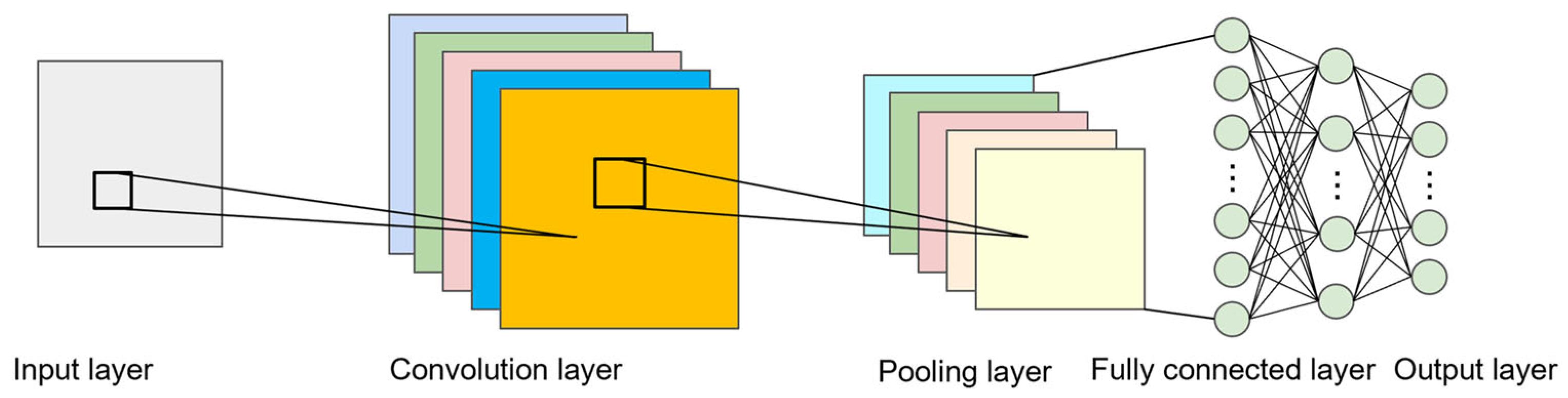
The convolutional neural network (CNN) is a deep learning architecture tailored to process grid-like data, such as images [37]. It has demonstrated significant success in various computer vision tasks, including image classification, object detection, and segmentation [38]. The core components of CNNs include convolutional layers, pooling layers, and fully connected layers, as shown in Figure 1, which together facilitate a hierarchical feature extraction.
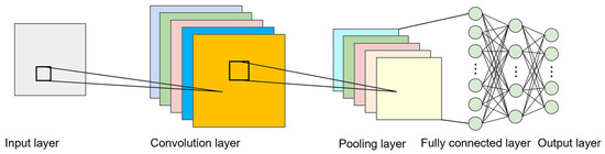
Figure 1.
The structure of a CNN.
The convolutional layer is the fundamental building block of a CNN. It applies a set of learnable filters (or kernels) to the input data to extract spatial features, such as edges, textures, and patterns. Given an input matrix and a filter , the convolution operation can be mathematically expressed as
where represents the output feature map at position , is the input region covered by the filter, is the filter weight matrix, is the bias term, and is the size of the filter.
The pooling layer reduces the spatial dimensions of feature maps while preserving their most important information. This helps to decrease the computational complexity and control overfitting. The most common pooling operation is max pooling, which takes the maximum value within a local receptive field:
After convolutional and pooling layers, the extracted feature maps are flattened into a one-dimensional vector and passed through fully connected (dense) layers. These layers perform high-level reasoning by learning complex feature relationships. The output of a fully connected layer is computed as
where represents the weight matrix, is the input vector, is the bias term, and is an activation function, typically ReLU or Softmax.
2.2. BiLSTM Model
Bidirectional long short-term memory (BiLSTM) is an advanced recurrent neural network (RNN) variant that enhances conventional LSTM by incorporating a bidirectional information flow [39]. This structure enables the model to capture both past and future contextual dependencies, making it highly effective for sequential data processing tasks, such as natural language processing, speech recognition, and time series forecasting.
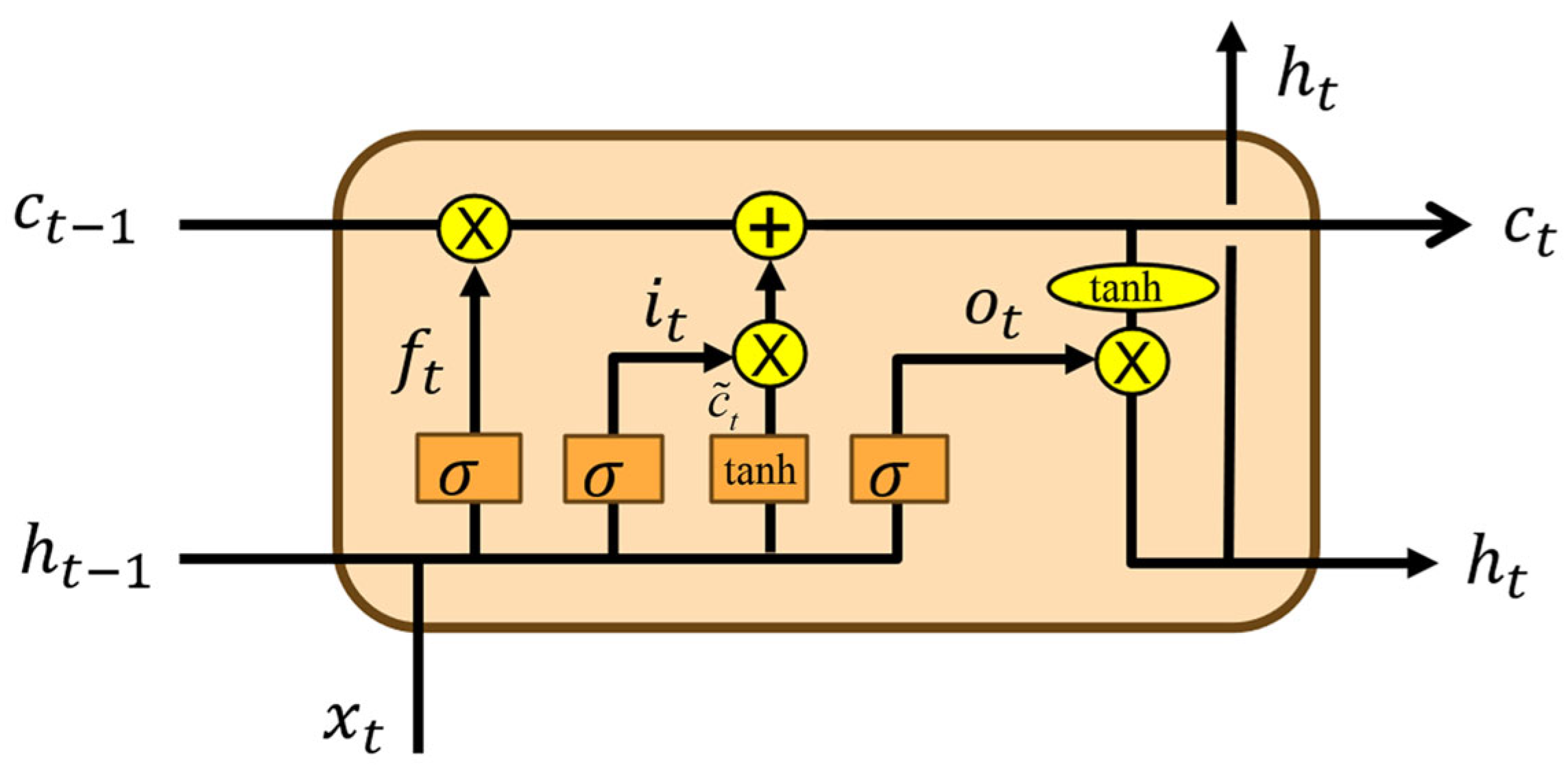
Long short-term memory (LSTM) networks were designed to address the vanishing gradient problem inherent in traditional RNNs, enabling them to effectively learn long-range dependencies [40]. Each LSTM unit consists of three primary gating mechanisms, the input gate, forget gate, and output gate, which regulate the flow of information within the network. The structure of LSTM is shown in Figure 2. Given an input sequence , the computation at time step is formulated as follows:
where denotes the sigmoid activation function; represents the element-wise multiplication; denotes the weight matrix between different nodes; denotes the bias vector; and , , and correspond to the activation values of the input gate, forget gate, and output gate, respectively. The cell state acts as a memory unit, and represents its candidate update, while represents the hidden state at time step .

Figure 2.
The structure of LSTM.
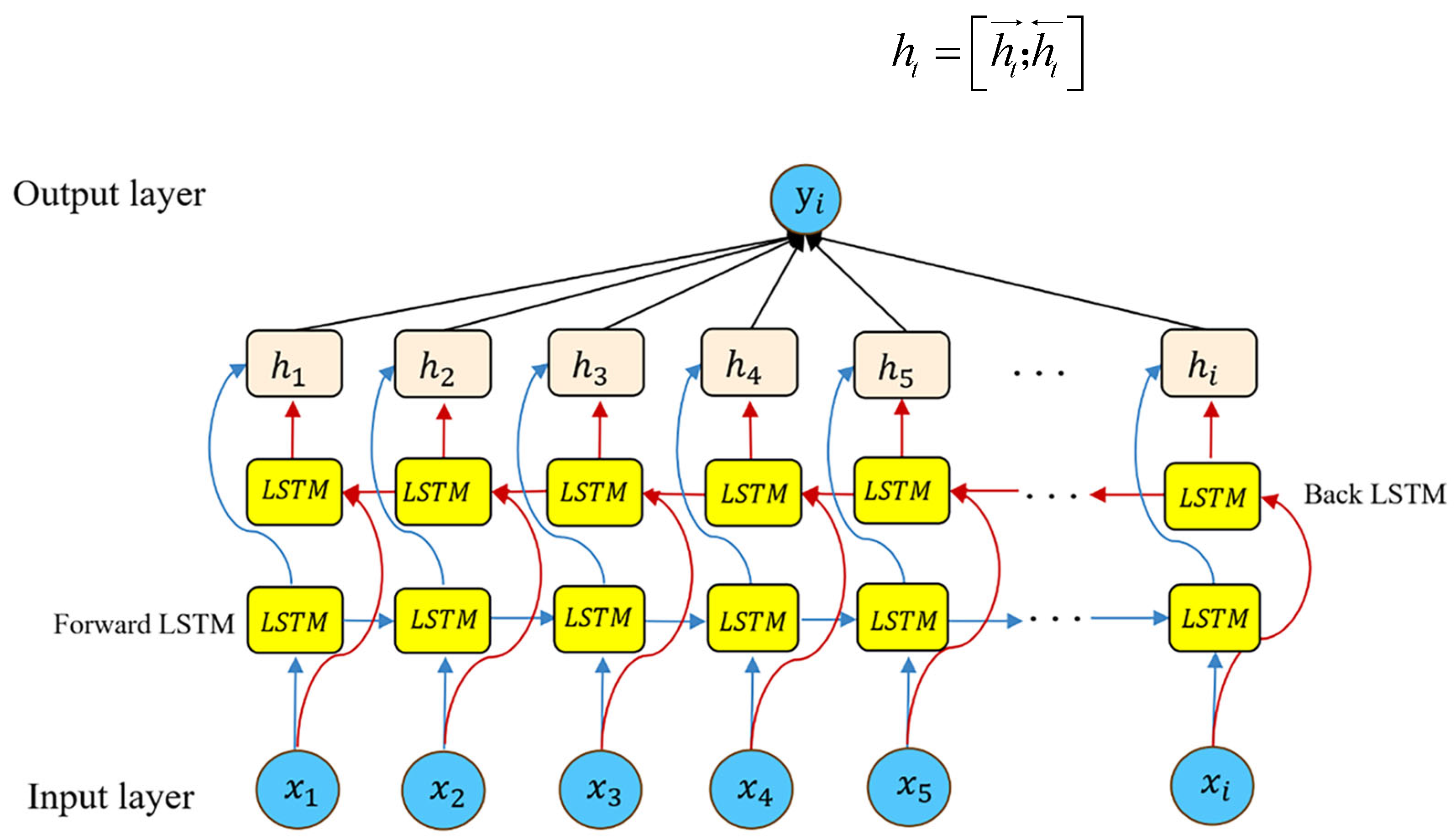
The standard LSTM processes sequences in a unidirectional manner, limiting its ability to leverage future contextual information. In contrast, BiLSTM employs two independent LSTM layers: a forward LSTM that processes the sequence from left to right and a backward LSTM that processes it from right to left [41]. Its structure is shown in Figure 3. Let and denote the hidden states produced by the forward and backward LSTM layers, respectively. The final hidden representation at time step is obtained through concatenation:
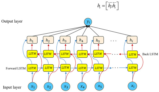
Figure 3.
The structure of BiLSTM.
2.3. Self-Attention Mechanism
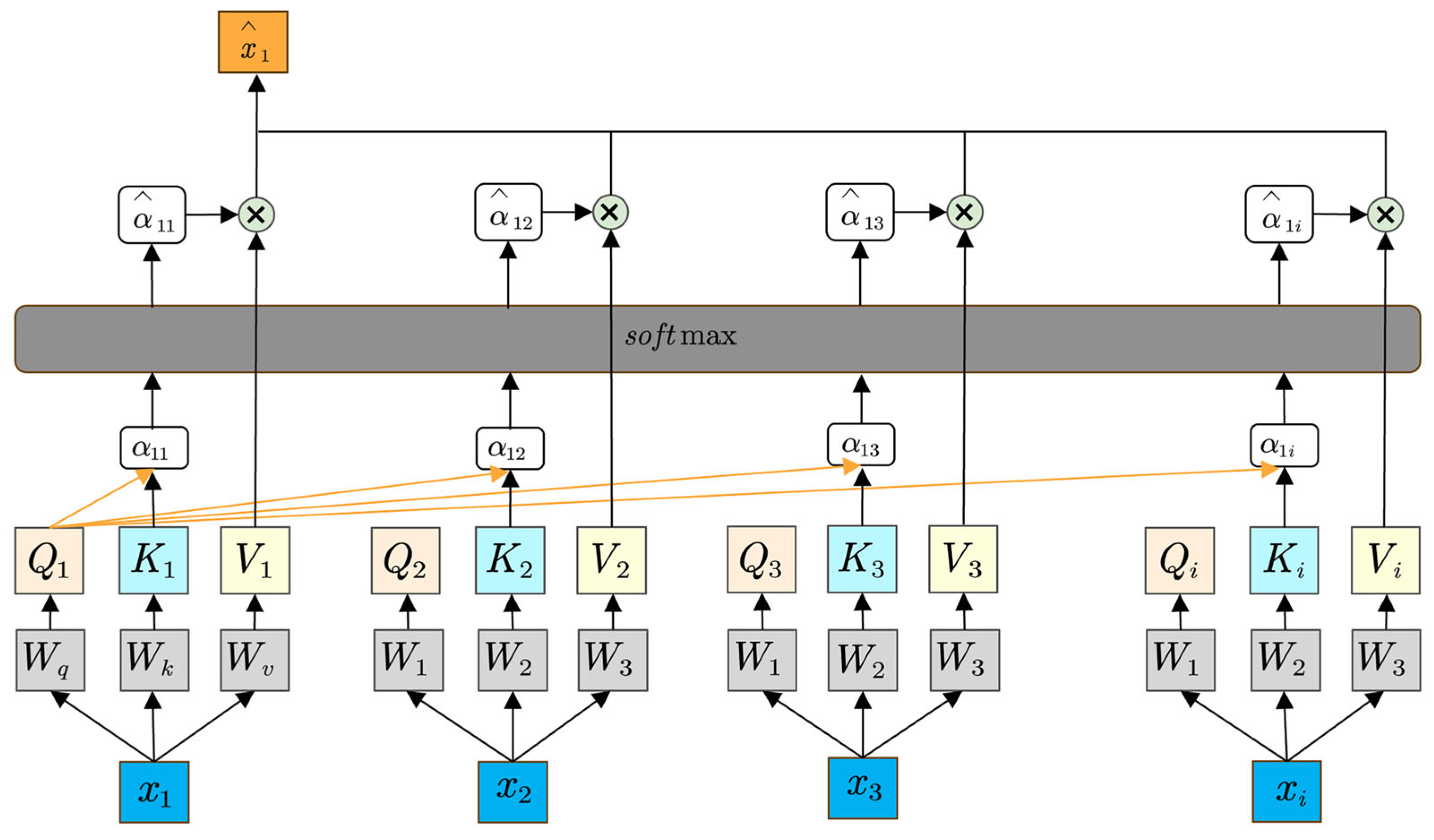
Self-attention is a powerful mechanism designed to capture contextual dependencies within a sequence by allowing each element to attend to all other elements [42]. Unlike traditional attention approaches that rely on encoder–decoder structures, self-attention applies the attention operation within a single sequence, thereby facilitating parallelization and reducing the distance between any two positions in the input [43]. This mechanism has become a cornerstone of Transformer-based models, demonstrating a superior performance in tasks such as machine translation, language modeling, and sequence classification. The model of the self-attention mechanism is shown in Figure 4.
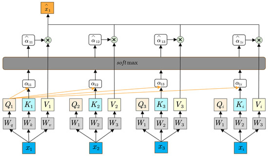
Figure 4.
The structure of the self-attention mechanism.
Self-attention mechanisms fundamentally rely on the interplay of three principal vectors: query (, key (), and value (). Given an input sequence , each token is projected into three distinct representations through learnable parameter matrices:
where , , and are the weight matrices for queries, keys, and values, respectively. These projections enable the model to encode different aspects of the input tokens, allowing each position to selectively focus on pertinent information from the entire sequence.
Once the query, key, and value vectors have been derived, the self-attention mechanism computes a weighted sum of the value vectors. Specifically, the similarity between a query and all keys is measured, typically via scaled dot product attention:
where represents the attention weight that token assigns to token , and denotes the dimensionality of the key vectors. The Softmax function normalizes the dot products into a probability distribution, ensuring that the weights sum to one. These weights are then used to form a weighted sum of the value vectors:
2.4. CNN-BiLSTM-SA Prediction Model
This hybrid architecture integrates the advantages of a convolutional neural network (CNN), bidirectional long short-term memory (BiLSTM) network, and self-attention mechanisms, enabling the precise prediction of multi-dimensional features in wind power data through systematic collaboration. Specifically, the CNN efficiently extracts local fluctuation features of wind speed data using 1D convolutional kernels. Its inherent translation equivariance and weight-sharing properties further effectively reduce the computational complexity. BiLSTM, in turn, captures long-term temporal dependencies through its bidirectional recursive structure, compensating for the CNN’s limitations in modeling long-range patterns. Together, the CNN and BiLSTM construct a hierarchical processing pipeline from “local feature extraction to global temporal modeling”. To address the intermittent nature of wind data, the introduced self-attention mechanism adaptively focuses on critical information points, such as strong wind events, and suppresses noise interference by dynamically calculating correlation weights between time steps. The explicit feature importance calibration provided by this mechanism complements the implicit temporal dependency modeling of BiLSTM, significantly enhancing the model’s robustness to outliers. Overall, this architecture substantially improves the wind power prediction performance through multi-dimensional feature collaborative processing (CNNs emphasizing spatial locality, BiLSTM handling temporal sequentiality, and self-attention optimizing feature weights) and parameter collaborative optimization.
As illustrated in Figure 5, our proposed model architecture comprises five sequential components: (1) an input layer for receiving multivariate time series data; (2) a CNN-based local feature extraction module; (3) a BiLSTM temporal modeling layer; (4) a self-attention feature weighting mechanism; and (5) a dense output layer for generating predictions. The structural design adheres to three core principles aimed at addressing specific challenges in wind power forecasting.
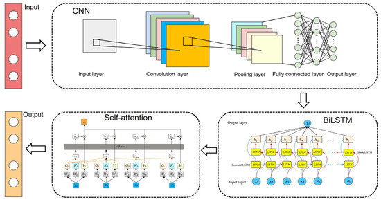
Figure 5.
CNN-BiLSTM-SA neural network.
In this study, the CNN module serves as the first-stage feature extractor, employing 1D convolutional kernels to capture local patterns within time series. The convolutional layer is configured with a specific number of kernels to extract local features across diverse temporal scales. Following convolution, batch normalization layers and ReLU activation functions are applied to enhance the training stability and nonlinear representation capabilities. A max-pooling layer then performs down-sampling along the temporal dimension, compressing the sequence length to reduce the subsequent computational complexity. To facilitate the effective integration with the BiLSTM, the model incorporates a sequence folding layer and a sequence unfolding layer: the former treats each time step of the input sequence as an independent sample, enabling parallel convolutional processing to improve the computational efficiency; the latter restores the feature sequence to its original structure after convolution, providing the input for the BiLSTM module.
The BiLSTM module receives the feature sequence processed by the CNN and captures both historical and future information through forward and backward LSTM units. Each LSTM unit contains input, forget, and output gates to handle long-range temporal dependencies. With a specified number of hidden units, the bidirectional processing outputs are obtained by concatenating the forward and backward hidden states, fully leveraging the bidirectional contextual information of the sequence. As a key component, the self-attention mechanism transforms the BiLSTM outputs via query, key, and value projection matrices, enabling the model to dynamically focus on critical segments within the sequence—which is particularly suitable for addressing the intermittent fluctuation characteristics in wind speed data. The output of the self-attention mechanism contains weighted feature representations for each time step. To generate the final prediction, the model first compresses the temporal dimension through global pooling to obtain a fixed-dimensional feature vector, which is then mapped to the specific prediction task via a fully connected layer.
3. An Optimized Escape Algorithm (OPESC)
3.1. Escape Algorithm
The escape algorithm (ESC) draws inspiration from the behavioral dynamics of human crowds during emergency evacuations, where individuals dynamically search for safe exits through adaptive interactions [44]. This algorithm emulates three distinct behavioral archetypes observed in evacuation scenarios: (1) the calm group, which rationally assesses environmental risks and guides the collective movement toward optimal paths, embodying systematic decision-making; (2) the flocking group, which engages in local exploration by mimicking the motion patterns of neighboring individuals, balancing cohesion and directional alignment; and (3) the panic group, which introduces the stochastic exploration of high-risk regions to enhance global diversity and prevent premature convergence.
By simulating the behaviors of these three groups, the algorithm balances exploration (global search) and exploitation (local optimization), effectively preventing the premature convergence to local optima.
3.1.1. Population Initialization
The ESC initializes a population of N individuals, where each individual is represented as a -dimensional vector:
Each dimension is initialized using a uniform random distribution:
After initialization, the fitness of each individual is evaluated, and individuals are sorted in ascending order based on fitness values. The top individuals are stored in an elite pool , representing the current optimal solutions (safe exits) that will guide subsequent iterations:
3.1.2. Panic Index
The panic index is introduced to model the time-varying emotional state of the crowd during the evacuation. Its value decreases as the iteration progresses:
A higher in the early stages promotes exploration, whereas a lower in later stages facilitates exploitation.
3.1.3. Exploration Phase
For , the algorithm remains in the exploration phase. The population is divided into three groups based on the fitness ranking, with proportions of (calm), (herding), and (panic).
- (1)
- Calm Group Update
Calm individuals move toward the group center while incorporating random perturbations:
- (2)
- Herding Group Update
Flocking individuals are influenced by both the calm and panic groups:
- (3)
- Panic Group Update
Panic individuals conduct random searches within both the elite pool and the population:
3.1.4. Exploitation Phase
For , the algorithm transitions to the exploitation phase, where all individuals are treated as calm and converge toward the elite pool and randomly selected individuals:
This phase enables fine-tuned adjustments to approximate the optimal solution.
3.1.5. Adaptive Lévy Weighting
Step size control is achieved through an adaptive Lévy weighting mechanism to balance exploration and exploitation dynamically:
In the early stages, a smaller encourages larger step sizes for exploration, while in later stages, a larger refines the search through smaller step sizes.
3.1.6. Fitness Evaluation and Elite Pool Update
At the end of each iteration, a greedy selection strategy retains superior solutions:
The elite pool E is dynamically updated to ensure that it always contains the historically best solutions.
3.2. Multi-Strategy Optimized Escape Algorithm
3.2.1. Log-Spiral Reverse Learning Initialization Strategy
In the ESC, the initial population is usually generated randomly, which can result in a non-uniform distribution of individuals across the solution space, raising the likelihood of the premature convergence to a local optimum. To address this issue and broaden the search space, this study introduces a strategy called Logarithmic Spiral Opposition-Based Learning (LsOBL). By combining the logarithmic spiral search path with opposition-based learning, LsOBL seeks to improve the global search ability of the algorithm and accelerate its convergence [45]. The formula is as follows:
3.2.2. Particle Swarm Optimization Strategy
Particle Swarm Optimization (PSO) is an optimization algorithm based on swarm intelligence, which simulates the social behavior of bird flocks to search for optimal solutions [46]. The PSO strategy is applied to update the individuals of the calm group, while using a linearly decreasing inertia weight and learning factors. This approach significantly enhances the algorithm’s global search capability and local search ability, making it suitable for solving various complex optimization problems. The formula is described as
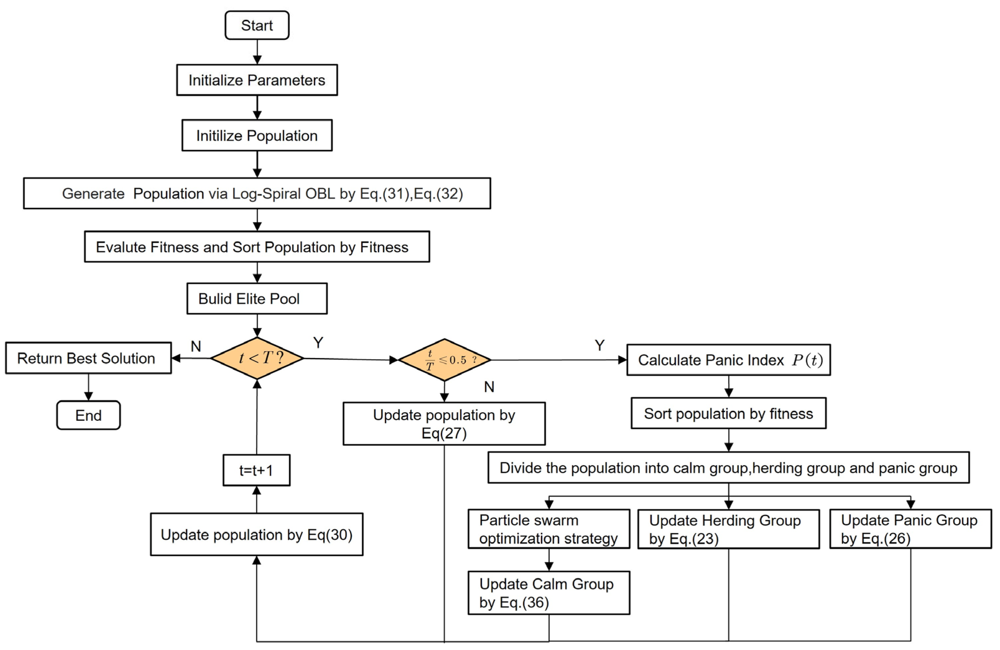
The parameters in Equations (14)–(36) are listed in Table 1. The flow of the OPESC is shown in Figure 6.

Table 1.
Parameter definition.
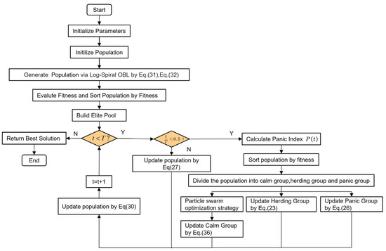
Figure 6.
The flowchart of the OPESC.
4. Performance Testing and Analysis of OPESC
4.1. Benchmark Test Functions
To further validate the performance of the OPESC, this study employs the CEC2017 benchmark function set for the evaluation. The CEC2017 suite comprises 29 complex functions, including unimodal, multimodal, hybrid, and composite types, which effectively simulate high-dimensional, nonlinear, and non-stationary optimization problems [47]. Among these, 10 representative functions were selected—hybrid functions F1–F5 and composite functions F6–F10—to comprehensively assess the algorithm’s global search capability, local exploitation efficiency, and dynamic adaptability. Detailed information regarding the test functions is provided in Table 2. The simulation environment comprises a Windows 11 64-bit operating system, 16 GB of RAM, and an Intel(R) Core (TM) i5-12500H@2.50 GHz CPU (Intel Corporation; Santa Clara, CA, USA). MATLAB R2024b is utilized as the simulation software.
Table 2.
Benchmark functions.
4.2. Comparison Algorithms and Parameter Settings
To evaluate the relative performance of the OPESC, it was compared with Differential Evolution (DE) [48], Particle Swarm Optimization (PSO) [46], the Crayfish Optimization Algorithm (COA) [49], the Gray Wolf Optimizer (GWO) [50], Harris Hawks Optimization (HHO) [51], the Whale Optimization Algorithm (WOA) [52], and the escape algorithm (ESC) [44]. A uniform parameter configuration was employed across all algorithms, with a population size of 100 and a fixed number of iterations set to 500.
4.3. Experimental Results
Table 3 presents a comparative analysis of various algorithms across 10 test functions, focusing on optimal values, mean values, and standard deviations. The OPESC exhibits a superior or comparable performance relative to other algorithms across several test functions.
Table 3.
A comparison of the OPESC and other algorithms on the CEC2017.
- (1)
- An Overall Comparison of Algorithm Performance: Based on the test results of hybrid functions (F1–F5) and composite functions (F6–F10), the OPESC demonstrates significant advantages across the majority of scenarios. Notably, the OPESC achieves the lowest optimal values in all ten test functions, highlighting its superior global search capability. For instance, in hybrid function F2, the OPESC obtains a best value of 2.56 × 10³, which is three orders of magnitude lower than DE’s 4.00 × 10⁶ and six orders lower than the WOA’s 2.14 × 10⁸. In composite function F10, the OPESC’s optimal value of 3.55 × 10³ outperforms the GWO’s 4.35 × 10³ and HHO’s 5.41 × 10³, further verifying its efficiency in escaping local optima.
- (2)
- The Trade-off Between Stability and Convergence: The comparative analysis reveals distinct trade-offs between the solution quality and stability among algorithms. The OPESC achieves optimal values that consistently outperform competitors while maintaining a dynamic equilibrium between exploration and exploitation—even with relatively high standard deviations (e.g., 5.34 × 10⁴ in F10). This balance enables the OPESC to escape local minima efficiently while controlling random fluctuations, as evidenced by its consistent attainment of high-quality solutions across functions.
In contrast, traditional algorithms like DE and PSO exhibit compromised stability–quality trade-offs. For instance, DE has a high standard deviation of 3.24 × 10⁹ in F4 alongside a best value of 1.69 × 10⁶, which is three orders of magnitude higher than the OPESC’s best value of 1.85 × 10³. Although PSO has a lower standard deviation (1.69 × 10⁹) in F4, it still fails to match the OPESC’s precision. The GWO and HHO further exemplify this limitation: in F3, the GWO’s standard deviation of 4.06 × 10⁶ accompanies a best value of 1.02 × 10⁶, which is significantly higher than the OPESC’s 1.18 × 10⁵. In summary, the OPESC not only achieves superior optimal values across most test functions but also demonstrates a strong competitive stability. Although there is still room for improvement in extremely high-dimensional or complex functions, this favorable balance between solution quality and stability endows the OPESC with a high potential for addressing multi-dimensional global optimization problems.
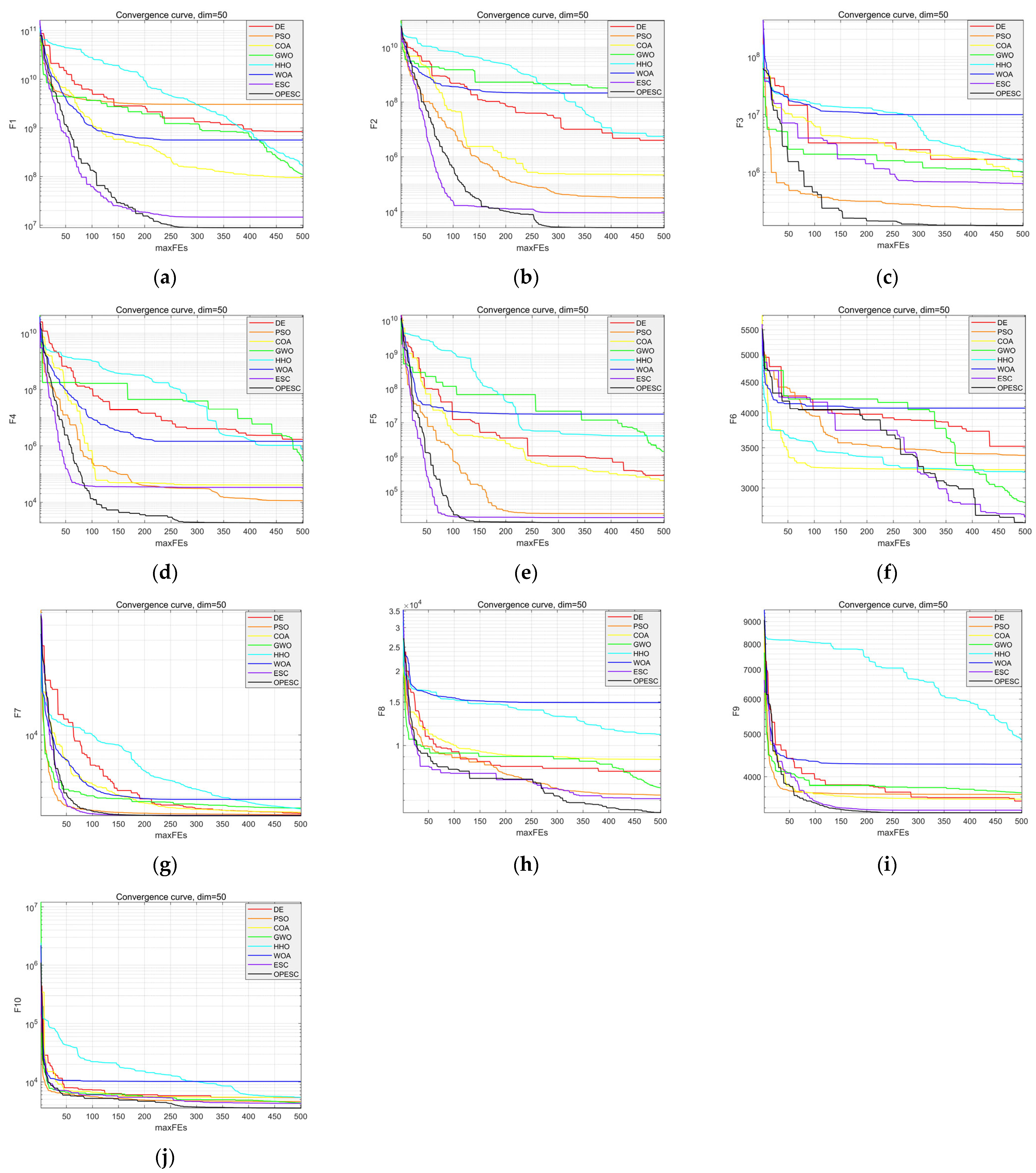
4.4. Convergence Curve Analysis
The convergence curves of various algorithms across ten test functions are illustrated in Figure 7. The OPESC convergence curve is smoother and consistently positioned lower than those of the other algorithms, indicating superior convergence behavior. In most test functions, the OPESC attains the optimal value within the first 300 iterations, underscoring its enhanced stability, higher convergence accuracy, and faster convergence speed.
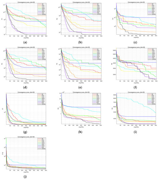
Figure 7.
Comparison chart of convergence of functions, (a) F1; (b) F2; (c) F3; (d) F4; (e) F5; (f) F6; (g) F7; (h) F8; (i) F9; and (j) F10.
5. Experiments
5.1. Data Description
This study utilizes a dataset derived from the Guohua Jingxia North Wind Farm in China, which has a capacity of 200 megawatts (MWs). The dataset includes operational data of wind turbine generator units collected from 00:00:00 on 1 January 2019 to 23:45:00 on 31 December 2019. With a sampling frequency of 15 min, a total of 35,040 raw data points are obtained, covering features such as wind speed, wind direction, air pressure, temperature, and humidity. Within this dataset, 2052 records (5.86% of the total) exhibit missing values across one or more features. To preserve temporal continuity and utilize sequential dependencies, a linear interpolation method is applied, where missing values are reconstructed by linearly fitting adjacent time-point observations.
A sliding window technique is employed to generate input–output sample pairs from the preprocessed time series, where each sample incorporates a contiguous 5-time-step historical feature vector as the input and the subsequent 1-time-step target value as the output. The window advances by 2 time steps per iteration, creating overlapping samples with 3-time-step shared data between consecutive instances to leverage temporal correlations effectively. This process theoretically generates a large number of samples, but to manage computational complexity, 2000 representative samples are selected from the full set. These samples are divided into a training set (1600 samples, 80%) and a testing set (400 samples, 20%) following the same temporal ordering principle, ensuring chronological consistency and unbiased model evaluation.
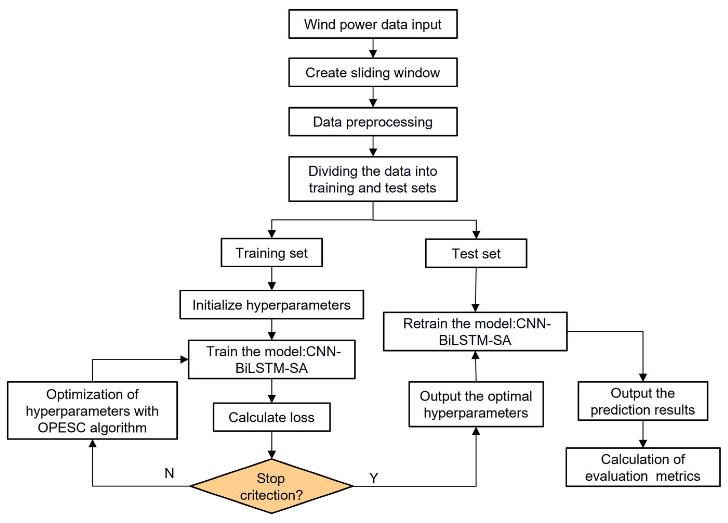
5.2. Algorithm Optimization Flow
In the proposed OPESC-CNN-BiLSTM-SA modeling framework, the wind power data are first processed using a sliding window method to generate input samples suitable for time series forecasting. Subsequently, following data preprocessing, the dataset is split into training and testing subsets. During the training phase, initial hyperparameters are specified, and the CNN-BiLSTM-SA model is trained while the loss function is evaluated. To further enhance the model’s performance, an improved ESC (OPESC) is introduced for hyperparameter optimization. When the optimization stopping criterion is not satisfied, OPESC continues to adjust the hyperparameters and retrain the model until the optimal condition is reached. Finally, the best-performing hyperparameters are employed to retrain the model on the testing set, producing the final predictions and enabling the computation of relevant evaluation metrics to assess the model’s predictive accuracy. The overall model framework is shown in Figure 8.

Figure 8.
The flowchart of the proposed OPESC-CNN-BiLSTM-SA model.
5.3. Experimental Configuration
The experimental hardware environment comprises a 12th Gen Intel(R) Core (TM) i5-12500H 2.50 GHz processor, equipped with 16 GB of RAM and 512 GB SSD storage, with MATLAB 2024b used as the software platform.
5.4. Model Training
The input data for this study comprises meteorological data from the wind farm collected over the past five time steps. The baseline model parameters are summarized in Table 4. The improved ESC was used for model parameter optimization and the number of iterations for each training session was set to 30. The OPESC was employed to optimize critical hyperparameters including the number of neurons, learning rate, and other architectural parameters, aiming to achieve optimal model performance. The optimization results of selected parameters for the OPESC-CNN-BiLSTM-SA model are systematically summarized in Table 5.
Table 4.
The baseline model parameters.
Table 5.
Optimized hyperparameters of model.
5.5. Evaluation Metric
The objective of the experiment is to predict the power generation of wind farms while maintaining high prediction accuracy in the testing dataset. Several key evaluation metrics have been established to assess the model’s performance, including Mean Squared Error (MSE), Root Mean Squared Error (RMSE), Mean Absolute Error (MAE), Mean Absolute Percentage Error (MAPE), Coefficient of Determination (R2), and Computational Time (CT). The formulas for these evaluation metrics are as follows:
where N represents the sample size, denotes the true data of the model at time , is the predicted value of the model at time , and represents the mean value of the true data.
5.6. Performance Assessment
5.6.1. Ablation Experiment
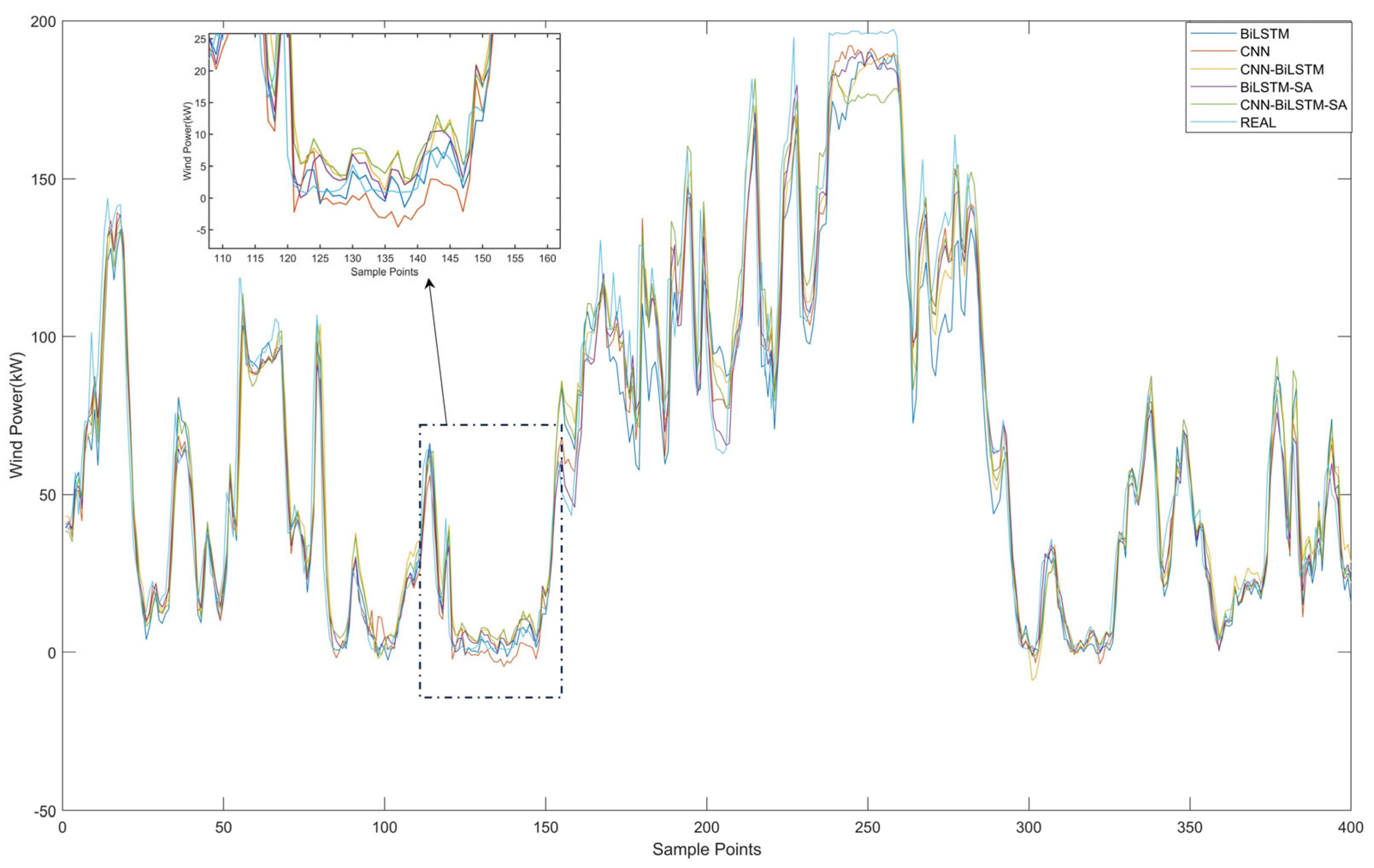
An ablation experiment was performed to evaluate component contributions in the CNN-BiLSTM-SA framework, comparing BiLSTM, CNN, CNN-BiLSTM, BiLSTM-SA, and CNN-BiLSTM-SA models. The experimental results are shown in Figure 9, and the evaluation metrics of the models are presented in Table 6.
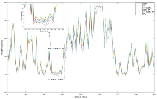
Figure 9.
Comparison of prediction results for different prediction models.
Table 6.
Comparison of evaluation metrics for different prediction models.
As illustrated in Figure 9, the prediction results of the CNN-BiLSTM-SA model are closer to the true values than other comparative models, validating its enhanced predictive accuracy and generalization capabilities. As shown in Table 6, the CNN-BiLSTM model demonstrated a 9.52% reduction in RMSE relative to BiLSTM, achieving 14.73 compared to 16.28, while MAE decreased by 4.51% to 10.79 from 11.30. This improvement, accompanied by an R2 increase to 93.16% from 91.44%, confirms convolutional layers’ efficacy in extracting spatial features to enhance temporal modeling. The standalone CNN achieved moderate performance with 15.77 RMSE and 11.15 MAE but exhibited limitations in temporal dependency modeling, evidenced by its 92.17% R2.
Integration of the self-attention mechanism with BiLSTM yielded a 6.45% RMSE reduction to 15.23 versus the BiLSTM baseline. However, this configuration increased MAPE to 12.51% from 12.16%, indicating inconsistent gains. When applied to CNN-BiLSTM, the attention mechanism produced more substantial improvements: RMSE decreased by 6.31% to 13.80 from 14.73, MAE reduced by 5.19% to 10.23 from 10.79, and R2 increased to 93.98%. These results demonstrate that attention mechanisms optimally enhance feature weighting only when processing high-quality spatiotemporal features.
In terms of Computational Time (CT), while the CNN-BiLSTM-SA model required 34.54 s, which was longer than that of some of the other models, its superior prediction accuracy justified the additional computational cost in scenarios where high precision was crucial.
By incorporating the OPESC, the predictive performance of the CNN-BiLSTM-SA model was significantly enhanced. The evaluation metric results are shown in Table 7. Compared to the original CNN-BiLSTM-SA model, the RMSE and MAE of the model utilizing the OPESC optimization were reduced to 9.65 and 6.70, respectively, representing reductions of 30.07% and 34.51%. Furthermore, the MSE decreased by 51.14% (from 190.50 to 93.14), indicating that the optimization algorithm effectively explored the hyperparameter space and enhanced the model’s generalization capability.
Table 7.
Performance comparison of CNN-BiLSTM-SA and OPESC-CNN-BiLSTM-SA models.
Notably, although the Computational Time (CT) of the OPESC-CNN-BiLSTM-SA model increased to 47.28 s, 37.29% longer than the 34.54 s of the original model, its remarkable boost in prediction accuracy makes the additional computational cost worthwhile, especially in applications where high precision is indispensable.
5.6.2. Comparative Experiments
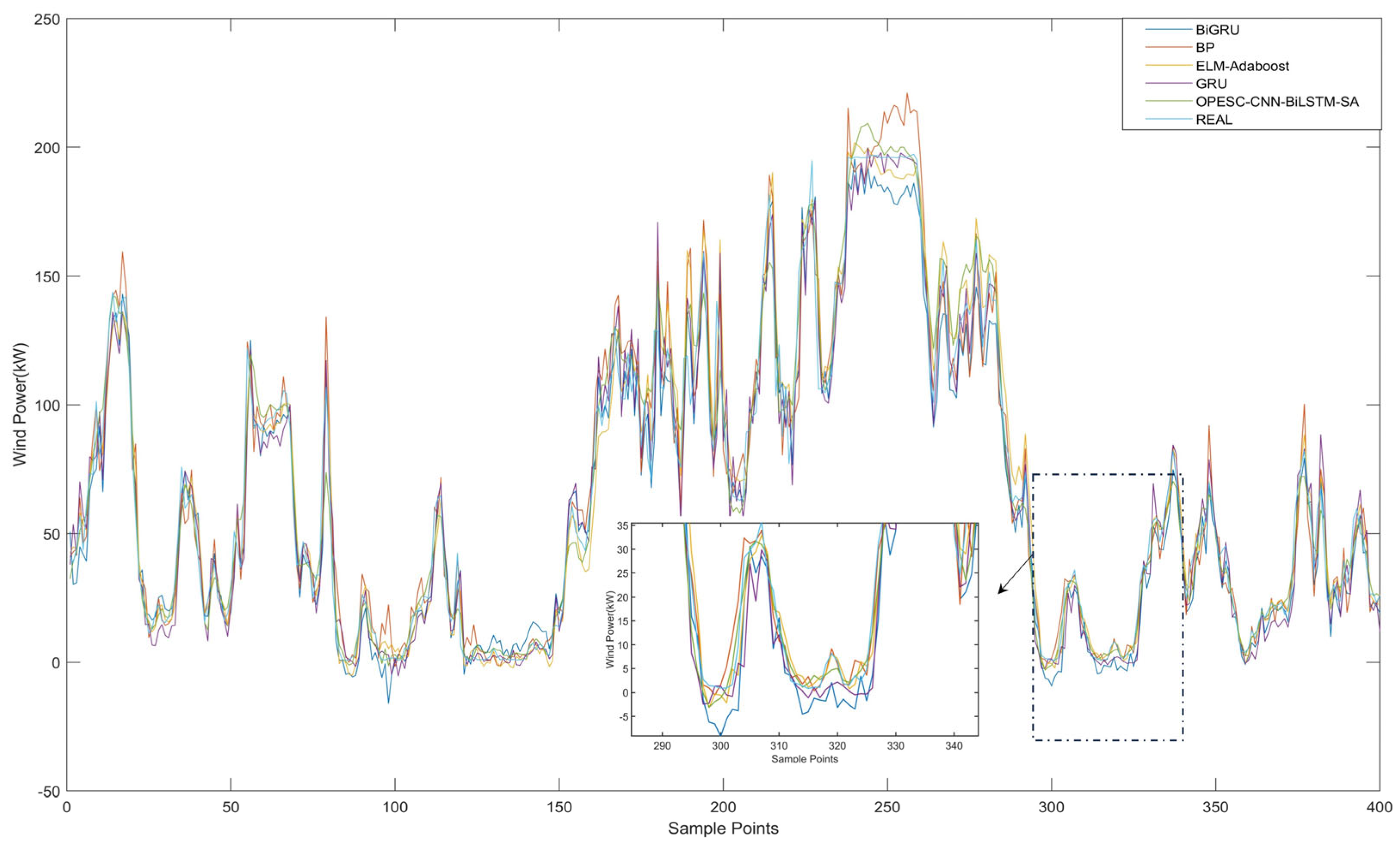
To verify the superiority of the OPESC-CNN-BiLSTM-SA model, this study introduced four additional prediction models: BP, BiGRU, ELM-Adaboost, and GRU. Figure 10 illustrates the prediction performance curves of these models, while Table 8 details their evaluation metrics. The experimental results demonstrate that the OPESC-CNN-BiLSTM-SA model outperforms all comparative models, as evidenced by its lowest RMSE of 9.65, lowest MAE of 6.70, and highest R2 of 97.06%.
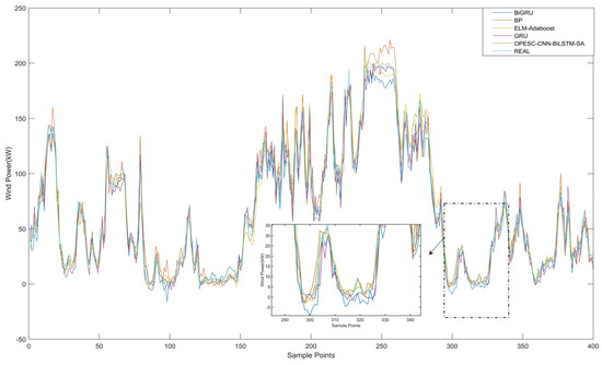
Figure 10.
Comparison of prediction results for diverse prediction models.
Table 8.
Comparison of evaluation metrics for diverse prediction models.
As shown in Figure 10, the prediction curve of the OPESC-CNN-BiLSTM-SA model exhibits the closest alignment with the true value curve across all data points, particularly in capturing complex fluctuation patterns. In contrast, other models such as BiGRU (RMSE = 11.41, MAE = 8.67) and GRU (RMSE = 11.64, MAE = 8.33) show more pronounced deviations in both steady and fluctuating regions, while BP (RMSE = 10.63, MAE = 7.27) and ELM-Adaboost (RMSE = 10.85, MAE = 7.46) display relatively smoother curves but still maintain larger gaps from the true values. The OPESC-CNN-BiLSTM-SA model’s superior performance is further validated by its lowest MAPE of 7.81%, indicating minimal relative prediction deviation compared to BP (8.57%), BiGRU (9.82%), ELM-Adaboost (8.34%), and GRU (8.96%).
6. Discussion and Conclusions
In the context of accelerating global energy transitions and the critical need for reliable renewable energy management, this study addresses the challenges posed by the nonlinear, non-stationary characteristics of wind dynamics, which complicate accurate wind power forecasting. A novel integrated framework, OPESC-CNN-BiLSTM-SA, is proposed, combining an optimized escape algorithm (OPESC) with a hybrid deep learning architecture to enhance the forecasting precision and facilitate an efficient grid integration. This research innovatively leverages optimization strategies and hierarchical neural network designs to overcome limitations in hyperparameter tuning, spatiotemporal feature extraction, and adaptive pattern modeling.
The principal conclusions are as follows:
- The OPESC, using logarithmic spiral opposition-based initialization and adaptive particle swarm strategies, outperforms classical methods (DE, PSO, etc.) in benchmark tests. Across 10 CEC2017 functions, it consistently achieves lower optimal values, escaping local optima to improve hyperparameter tuning for complex models.
- The OPESC-optimized CNN-BiLSTM-SA reduces the RMSE by 30.07%, the MAE by 34.51%, and the MAPE by 7.81% on real wind data. With an R2 of 97.06%, it robustly models intermittent wind dynamics, highlighting the role of intelligent optimization in deep learning.
- The hybrid model combines a CNN for the spatial feature extraction, BiLSTM for bidirectional temporal dependencies, and self-attention for dynamic weighting. This design captures meteorological correlations, historical/future trends, and critical time steps, outperforming standalone models in handling non-stationary data.
- Validated in wind farms, the framework cuts key errors by 30–35%, enabling a reliable grid dispatch, cost-effective storage, and reduced supply–demand risks. It supports low-carbon transitions by improving renewable predictability, a vital factor for global energy integration.
The OPESC’s adaptability and the CNN-BiLSTM-SA model’s robust feature processing make the framework applicable to broader energy forecasting scenarios, including solar and hybrid energy systems, where similar challenges of non-stationarity and intermittency exist. This study not only advances the state of wind power forecasting but also provides a novel research paradigm for integrating intelligent optimization with deep learning in energy systems.
Despite its promising results, this study has several limitations warranting consideration. Firstly, the model’s validation relies primarily on data from a single wind farm, raising questions about its generalizability to geographically diverse sites with distinct meteorological profiles. Secondly, while effective, the OPESC exhibits significant computational complexity, particularly in extremely high-dimensional optimization spaces, posing challenges for large-scale applications. Finally, the deployment of real-time forecasting necessitates addressing this computational overhead and exploring its integration with edge computing platforms to enhance the operational feasibility. To address these gaps, future research will focus on three key directions: (1) extending the framework to multi-step-ahead forecasting and multi-wind farm collaborative modeling, leveraging graph neural networks to capture spatial dependencies across geographically distributed energy systems; (2) optimizing the OPESC for high-dimensional scenarios through dimensionality reduction techniques and edge computing integration, enabling real-time hyperparameter tuning with a reduced computational overhead; and (3) incorporating multi-source data fusion mechanisms and lightweight model architectures to improve the scalability and adaptability for large-scale, real-time energy management systems.
Author Contributions
Conceptualization, L.W.; methodology, L.W.; software, L.W.; validation, L.W.; data curation, L.W.; visualization, L.W.; writing—original draft preparation, L.W.; investigation, L.W.; D.Z.; writing—review and editing, D.Z.; supervision, D.Z.; project administration, D.Z. All authors have read and agreed to the published version of the manuscript.
Funding
This research received no external funding.
Data Availability Statement
The original contributions presented in this study are included in the article. Further inquiries can be directed to the corresponding authors.
Conflicts of Interest
The authors declare no conflicts of interest.
References
- Petersen, C.; Reguant, M.; Segura, L. Measuring the impact of wind power and intermittency. Energy Econ. 2024, 129, 107200. [Google Scholar] [CrossRef]
- Chen, J.; Zeng, G.-Q.; Zhou, W.; Du, W.; Lu, K.-D. Wind speed forecasting using nonlinear-learning ensemble of deep learning time series prediction and extremal optimization. Energy Convers. Manag. 2018, 165, 681–695. [Google Scholar] [CrossRef]
- Qu, Z.; Hou, X.; Huang, S.; Li, D.; He, Y.; Meng, Y. Probabilistic power forecasting for wind farm clusters using Moran-Graph network with posterior feedback attention mechanism. Energy 2025, 328, 136558. [Google Scholar] [CrossRef]
- Dai, X.; Liu, G.-P.; Hu, W. An online-learning-enabled self-attention-based model for ultra-short-term wind power forecasting. Energy 2023, 272, 127173. [Google Scholar] [CrossRef]
- Zhang, Q.; Liu, Y.; Zhou, J.; Lei, B.; Liu, Y.; Wang, Y. A Review of Emerging Trends in Wind Power Forecasting Applications. In Proceedings of the 9th International Conference on Power and Renewable Energy, Guangzhou, China, 20–23 September 2024; pp. 1396–1401. [Google Scholar]
- Zhao, Z.; Xu, J.; Lei, Y.; Liu, C.; Shi, X.; Lai, L.L. Robust dynamic dispatch strategy for multi-uncertainties integrated energy microgrids based on enhanced hierarchical model predictive control. Appl. Energy 2025, 381, 125141. [Google Scholar] [CrossRef]
- Wang, C.; Wang, M.; Wang, A.; Zhang, X.; Zhang, J.; Ma, H.; Yang, N.; Zhao, Z.; Lai, C.S.; Lai, L.L. Multiagent deep reinforcement learning-based cooperative optimal operation with strong scalability for residential microgrid clusters. Energy 2025, 314, 134165. [Google Scholar] [CrossRef]
- Aziz, A.; Than Oo, A.; Stojcevski, A. Frequency regulation capabilities in wind power plant. Sustain. Energy Technol. Assess. 2018, 26, 47–76. [Google Scholar] [CrossRef]
- Wei, Z.N.; Zhao, D. Efficient Short-Term Wind Power Prediction Using a Novel Hybrid Machine Learning Model: LOFVT-OVMD-INGO-LSSVR. Energies 2025, 18, 1849. [Google Scholar] [CrossRef]
- Dupre, A.; Drobinski, P.; Alonzo, B.; Badosa, J.; Briard, C.; Plougonven, R. Sub-hourly forecasting of wind speed and wind energy. Renew. Energy 2020, 145, 2373–2379. [Google Scholar] [CrossRef]
- Tian, S.; Fu, Y.; Ling, P.; Wei, S.; Liu, S.; Li, K. Wind Power Forecasting Based on ARIMA-LGARCH Model. In Proceedings of the 2018 International Conference on Power System Technology (POWERCON), Guangzhou, China, 6–8 November 2018; pp. 1285–1289. [Google Scholar]
- Ahmadi, M.; Khashei, M. Current status of hybrid structures in wind forecasting. Eng. Appl. Artif. Intell. 2021, 99, 104133. [Google Scholar] [CrossRef]
- Liu, C.; Zhang, X.; Mei, S.; Zhen, Z.; Jia, M.; Li, Z.; Tang, H. Numerical weather prediction enhanced wind power forecasting: Rank ensemble and probabilistic fluctuation awareness. Appl. Energy 2022, 313, 118769. [Google Scholar] [CrossRef]
- Al-Yahyai, S.; Charabi, Y.; Gastli, A. Review of the use of Numerical Weather Prediction (NWP) Models for wind energy assessment. Renew. Sustain. Energy Rev. 2010, 14, 3192–3198. [Google Scholar] [CrossRef]
- Wang, J.; Qian, Y.; Zhang, L.; Wang, K.; Zhang, H. A novel wind power forecasting system integrating time series refining, nonlinear multi-objective optimized deep learning and linear error correction. Energy Convers. Manag. 2024, 299, 117818. [Google Scholar] [CrossRef]
- Li, C.; Cao, D.-S.; Zhao, Z.-T.; Wang, X.; Xie, X.-Y. Forecast for wind power at ultra-short-term based on a composite model. Energy Rep. 2024, 12, 4076–4082. [Google Scholar] [CrossRef]
- Wang, J.; Zhou, Q.; Zhang, X. Wind power forecasting based on time series ARMA model. In Proceedings of the 1st International Conference on Environment Prevention and Pollution Control Technology (EPPCT), Tokyo, Japan, 9–11 November 2018. [Google Scholar]
- Tian, Z.; Li, H.; Li, F. A combination forecasting model of wind speed based on decomposition. Energy Rep. 2021, 7, 1217–1233. [Google Scholar] [CrossRef]
- Guo, Z.-h.; Wu, J.; Lu, H.-y.; Wang, J.-z. A case study on a hybrid wind speed forecasting method using BP neural network. Knowl.-Based Syst. 2011, 24, 1048–1056. [Google Scholar] [CrossRef]
- Shahid, F.; Zameer, A.; Muneeb, M. A novel genetic LSTM model for wind power forecast. Energy 2021, 223, 120069. [Google Scholar] [CrossRef]
- Zhu, A.; Li, X.; Mo, Z.; Wu, R. Wind power prediction based on a convolutional neural network. In Proceedings of the 2017 International Conference on Circuits, Devices and Systems (ICCDS), Chengdu, China, 5–8 September. 2017; pp. 131–135. [Google Scholar]
- Chen, Y.; Zhao, H.; Zhou, R.; Xu, P.; Zhang, K.; Dai, Y.; Zhang, H.; Zhang, J.; Gao, T. CNN-BiLSTM Short-Term Wind Power Forecasting Method Based on Feature Selection. IEEE J. Radio. Freq. Identif. 2022, 6, 922–927. [Google Scholar] [CrossRef]
- Zhang, R.; Bu, S.; Zheng, Y.; Li, G.; Wan, X.; Zeng, Q.; Zhou, M. A novel multi-task learning model based on Transformer-LSTM for wind power forecasting. Int. J. Electr. Power Energy Syst. 2025, 169, 110732. [Google Scholar] [CrossRef]
- Zhao, Z.; Yun, S.; Jia, L.; Guo, J.; Meng, Y.; He, N.; Li, X.; Shi, J.; Yang, L. Hybrid VMD-CNN-GRU-based model for short-term forecasting of wind power considering spatio-temporal features. Eng. Appl. Artif. Intell. 2023, 121, 105982. [Google Scholar] [CrossRef]
- Ye, J.; Dai, L.; Wang, H. Enhancing sewage flow prediction using an integrated improved SSA-CNN-Transformer-BiLSTM model. Aims Math. 2024, 9, 26916–26950. [Google Scholar] [CrossRef]
- Huan, S. A novel interval decomposition correlation particle swarm optimization-extreme learning machine model for short-term and long-term water quality prediction. J. Hydrol. 2023, 625, 130034. [Google Scholar] [CrossRef]
- Guan, S.; Wang, Y.; Liu, L.; Gao, J.; Xu, Z.; Kan, S. Ultra-short-term wind power prediction method based on FTI-VACA-XGB model. Expert. Syst. Appl. 2024, 235, 121185. [Google Scholar] [CrossRef]
- Geng, L.; Zhang, L.; Niu, F.; Li, Y.; Liu, F. A swarm intelligence and deep learning strategy for wind power and energy storage scheduling in smart grid. Int. J. Intell. Netw. 2024, 5, 302–314. [Google Scholar] [CrossRef]
- Gao, X.; Guo, W.; Mei, C.; Sha, J.; Guo, Y.; Sun, H. Short-term wind power forecasting based on SSA-VMD-LSTM. Energy Rep. 2023, 9, 335–344. [Google Scholar] [CrossRef]
- Lu, P.; Ye, L.; Zhong, W.; Qu, Y.; Zhai, B.; Tang, Y.; Zhao, Y. A novel spatio-temporal wind power forecasting framework based on multi-output support vector machine and optimization strategy. J. Clean. Prod. 2020, 254, 119993. [Google Scholar] [CrossRef]
- Li, L.-L.; Zhao, X.; Tseng, M.-L.; Tan, R.R. Short-term wind power forecasting based on support vector machine with improved dragonfly algorithm. J. Clean. Prod. 2020, 242, 118447. [Google Scholar] [CrossRef]
- Barman, M.; Choudhury, N.B.D.; Sutradhar, S. A regional hybrid GOA-SVM model based on similar day approach for short-term load forecasting in Assam, India. Energy 2018, 145, 710–720. [Google Scholar] [CrossRef]
- Liu, Z.; Ge, H.; Song, T.; Ma, S. Research on building energy-saving based on GA-BP coupled improved multi-objective whale optimization algorithm. Energy Build. 2025, 328, 115141. [Google Scholar] [CrossRef]
- Su, W.; Jin, G.; Xiang, R.; Yang, Y.; Qiu, M.; Zhao, Z.; Zhao, Q. Prediction of flow stress and research of the hot working diagram for 4Cr5Mo2V steel based on the Arrhenius and the improved PSO-BP. Mater. Today Commun. 2025, 46, 112673. [Google Scholar] [CrossRef]
- Shang, M.; Yuan, R.; Song, B.; Huang, X.; Yang, B.; Li, S. Joint observation and transmission scheduling of multiple agile satellites with energy constraint using improved ACO algorithm. Acta Astronaut. 2025, 230, 92–103. [Google Scholar] [CrossRef]
- Zhang, P.; Sun, C.; Xia, X.-L. Improved Gold-SA algorithm for simultaneous estimation of temperature-dependent thermal conductivity and spectral radiative properties of semitransparent medium. Int. J. Heat Mass. Transf. 2022, 191, 122836. [Google Scholar] [CrossRef]
- Li, Z.; Liu, F.; Yang, W.; Peng, S.; Zhou, J. A Survey of Convolutional Neural Networks: Analysis, Applications, and Prospects. Ieee Trans. Neural Netw. Learn. Syst. 2022, 33, 6999–7019. [Google Scholar] [CrossRef]
- Aloysius, N.; Geetha, M. A review on deep convolutional neural networks. In Proceedings of the 2017 International Conference on Communication and Signal Processing (ICCSP), Chennai, India, 6–8 April 2017; pp. 0588–0592. [Google Scholar]
- Petrosanu, D.-M.; Pirjan, A. Electricity Consumption Forecasting Based on a Bidirectional Long-Short-Term Memory Artificial Neural Network. Sustainability 2021, 13, 104. [Google Scholar] [CrossRef]
- Ma, J.; Liu, H.; Peng, C.; Qiu, T. Unauthorized Broadcasting Identification: A Deep LSTM Recurrent Learning Approach. Ieee Trans. Instrum. Meas. 2020, 69, 5981–5983. [Google Scholar] [CrossRef]
- Li, Y.; Huang, W.; Lou, K.; Zhang, X.; Wan, Q. Short-term PV power prediction based on meteorological similarity days and SSA-BiLSTM. Syst. Soft Comput. 2024, 6, 200084. [Google Scholar] [CrossRef]
- Huang, Z.; Liang, M.; Qin, J.; Zhong, S.; Lin, L. Understanding Self-attention Mechanism via Dynamical System Perspective. In Proceedings of the 2023 IEEE/CVF International Conference on Computer Vision (ICCV), Paris, France, 1–6 October. 2023; pp. 1412–1422. [Google Scholar]
- Wan, A.; Chang, Q.; Al-Bukhaiti, K.; He, J. Short-term power load forecasting for combined heat and power using CNN-LSTM enhanced by attention mechanism. Energy 2023, 282, 128274. [Google Scholar] [CrossRef]
- Ouyang, K.; Fu, S.; Chen, Y.; Cai, Q.; Heidari, A.A.; Chen, H. Escape: An optimization method based on crowd evacuation behaviors. Artif. Intell. Rev. 2024, 58, 19. [Google Scholar] [CrossRef]
- Geng, J.; Sun, X.; Wang, H.; Bu, X.; Liu, D.; Li, F.; Zhao, Z. A modified adaptive sparrow search algorithm based on chaotic reverse learning and spiral search for global optimization. Neural Comput. Appl. 2023, 35, 24603–24620. [Google Scholar] [CrossRef]
- Kennedy, J.; Eberhart, R. Particle swarm optimization. In Proceedings of the 1995 IEEE International Conference on Neural Networks (ICNN 95), Perth, Australia, 27 November–1 December 1995; pp. 1942–1948. [Google Scholar]
- Kommadath, R.; Kotecha, P. Teaching Learning Based Optimization with focused learning and its performance on CEC2017 functions. In Proceedings of the 2017 IEEE Congress on Evolutionary Computation (CEC), Donostia, Spain, 5–8 June 2017; pp. 2397–2403. [Google Scholar]
- Storn, R.; Price, K. Differential evolution—A simple and efficient heuristic for global optimization over continuous spaces. J. Glob. Optim. 1997, 11, 341–359. [Google Scholar] [CrossRef]
- Jia, H.; Rao, H.; Wen, C.; Mirjalili, S. Crayfish optimization algorithm. Artif. Intell. Rev. 2023, 56, 1919–1979. [Google Scholar] [CrossRef]
- Mirjalili, S.; Mirjalili, S.M.; Lewis, A. Grey Wolf Optimizer. Adv. Eng. Softw. 2014, 69, 46–61. [Google Scholar] [CrossRef]
- Heidari, A.A.; Mirjalili, S.; Faris, H.; Aljarah, I.; Mafarja, M.; Chen, H. Harris hawks optimization: Algorithm and applications. Future Gener. Comput. Syst. 2019, 97, 849–872. [Google Scholar] [CrossRef]
- Mirjalili, S.; Lewis, A. The Whale Optimization Algorithm. Adv. Eng. Softw. 2016, 95, 51–67. [Google Scholar] [CrossRef]

Disclaimer/Publisher’s Note: The statements, opinions and data contained in all publications are solely those of the individual author(s) and contributor(s) and not of MDPI and/or the editor(s). MDPI and/or the editor(s) disclaim responsibility for any injury to people or property resulting from any ideas, methods, instructions or products referred to in the content. |
© 2025 by the authors. Licensee MDPI, Basel, Switzerland. This article is an open access article distributed under the terms and conditions of the Creative Commons Attribution (CC BY) license (https://creativecommons.org/licenses/by/4.0/).