Abstract
Transcatheter aortic valve replacement (TAVR) is a high-risk cardiovascular interventional procedure with a high incidence of postoperative complications, urgently requiring more refined risk identification and mitigation strategies. The main challenges in assessing the risk of TAVR complications lie in the scarcity of real-world data and the co-occurrence of multiple complications. This study developed an adjustment evaluation model that adapts randomised clinical trial (RCT) evidence to real-world data (RWD) and adopted multi-label classification methods that incorporate a LocalGLMnet-like regularization term, enabling data-adaptive parameter shrinkage for more accurate estimation. In the empirical analysis, with real surgical data from a hospital in the United States, a combination of multi-label random sampling and representative multi-label classification algorithms was used to fit the data. The model was compared across multiple evaluation metrics, including Hamming loss, ranking loss, and micro-AUC, to ensure robust results. The model used in this paper bridges the gap between medical risk prediction and insurance actuarial science, provides a practical data modelling foundation and algorithmic support for the future development of post-operative complication insurance products that precisely align with clinical risk.
MSC:
62P10
1. Introduction
Multi-label classification (MLC) is a common and important task in machine learning [1], it is characterized by the fact that each sample may belong to more than one label at the same time. Let the training data set be , where is the characteristic vector of the sample i. is the corresponding label indication vector. Each component indicates that the sample is correlated with the label in label sets . The goal of MLC is to learn a mapping function , which enables it to predict the corresponding set of relevant labels for any unknown sample . In contrast to traditional single-label classification or multi-class classification tasks, multi-label learning requires not only dealing with high-dimensional output spaces but also modelling the potential correlations and dependencies between labels. In medical diagnosis, an individual may suffer from multiple diseases at the same time, and predicting the risk of several normal diseases at the same time is challenging.
There are typically two approaches to addressing MLC problems: problem transformation and algorithm adaptation. Problem transformation methods convert MLC into single-label classification [1] or label ranking problems [2]. Among these, binary relevance (BR) treats each label as an independent binary classification task and trains multiple single-label classifiers for prediction [3]; label powerset (LP) treats different label combinations as new categories, converting multi-label data into a multi-class dataset and then mapping the prediction results back to the original label space after training [4]; and classifier chains (CC) introduce label relevance, using a chained structure to pass label information to improve prediction performance [5]. The second-order method, calibrated label ranking (CLR), transforms multi-label learning tasks into label ranking tasks [2] while random k-label sets (RAkELs) transform multi-label learning tasks into multi-class classification tasks [6].
Another main approach is algorithm adaptation, which involves modifying traditional classification algorithms to directly handle multi-label data. Such methods typically require multi-label-specific modifications to the base algorithm, such as adjusting decision boundaries, loss functions, or feature representations, to better capture the complex relationships between labels. In existing research, several classic algorithms have been successfully extended to multi-label scenarios, including multi-label k-nearest neighbours (ML-kNN) [7], multiclass multi-label perceptrons (MMP) [8], and ranked support vector machines (rank-SVM) [9].
A major problem associated with MLC is label imbalance. The imbalance of labels increases when the number of labels is large and the average number of labels associated with each instance is small. In this case, the level of imbalance of label i can be measured by the label imbalance ratio (), which is defined as the ratio of the number of instances associated to the most frequently occurring label to the number of instances associated to label i [10], where
The level of imbalance in a multi-labelled dataset can be measured by , which is averaged over all labels:
A larger value of indicates a higher degree of imbalance for the label i, while the larger value of indicates a higher degree of imbalance for the entire data set.
The solutions proposed for addressing imbalanced data in MLC can be categorised into four types [11]: resampling methods [12], classifier adaptation [13,14,15], ensemble methods [16,17], and cost-sensitive methods [18,19]. Resampling methods are the most commonly used techniques for handling imbalanced data. The goal is to generate a new, more balanced MLD dataset. Resampling methods typically achieve this through undersampling, which involves removing samples associated with the majority label [20], or oversampling, which involves generating new samples associated with the minority label [21]. These methods can also be categorised into two types: random methods and heuristic methods, based on whether new samples are removed or generated.
Random resampling methods for MLC can be based on LP conversion, BR methods, imbalance measures, etc. For example, LPRUS and LPROS are based on LP conversion [2]. The LP conversion method transforms an MLD into a multi-class classification problem, where each unique label combination is regarded as a new class. The undersampling strategy LP-RUS, based on this method, reduces category distribution imbalance by randomly removing samples belonging to the most frequent label sets until the total number of samples is reduced to a predefined threshold. LP-ROS, on the other hand, randomly replicates samples belonging to rare label sets to expand the dataset until the predefined total sample size is reached, thereby alleviating the problem of insufficient minority class samples. MLRUS and MLROS do not process the complete label set frequency but instead operate on the occurrence frequency of individual labels. By identifying and processing samples containing one or more minority class labels, they achieve mitigation of the imbalance problem [22]. Both methods rely on the label imbalance indicators and . When the value of a label is greater than , the label is considered a minority class; otherwise, it is considered a majority class. To address the issue of minority labels often co-occurring with majority labels in the same sample, a new resampling method called REMEDIAL was proposed [23]. The REMEDIAL method decouples majority and minority labels to address the imbalance problem, and this method can be used as an independent sampling method or combined with other resampling techniques.
Previous studies have applied multi-label classification methods to the medical field. For example, in the prediction of diabetes complications, various classical multi-label classification methods have been used [24]. In the prediction of chronic diseases, novel multi-label neural network methods [25], deep learning-based methods [26], and the Ensemble Label Power Set Pruning Data Set Joint Decomposition method [27] have been proposed. Since the first TAVR procedure was performed by French doctors in 2002, it has gradually become a major treatment method for patients with severe, symptomatic aortic valve stenosis [28]. Clinical results show that TAVR surgery is associated with a risk of complications. Despite continuous technological advancements in recent years, the incidence of TAVR-related complications remains high. Given that a single patient may experience multiple complications concurrently after TAVR surgery, this inherently constitutes a typical MLC problem. However, current research has not yet systematically applied MLC methods to the prediction and determination of TAVR surgical complication categories. To bridge this research gap, this paper will utilize TAVR surgical complication data from a US hospital, comprehensively considering individual inherent attributes, hospital attributes, and prior medical history from multiple dimensions to predict postoperative complications. Addressing the inherent imbalanced MLC nature of the data, this study will employ random resampling techniques and classical MLC methods for data processing and incidence prediction analysis.
The influence of covariates on various response variables differs in magnitude, and their importance is not uniform. Given this, introducing shrinkage estimation methods is crucial for identifying and quantifying these differential impacts, enabling effective feature selection, and enhancing model generalisation capabilities. LocalGLMnet is a regularised estimation method based on Generalised Linear Models (GLMs). It tackles the limitations of traditional GLMs with high-dimensional, complex local data by fitting GLMs within local neighbourhoods and applying Elastic Net regularisation for variable selection and parameter estimation [29]. Research shows that incorporating regularisation like group lasso within LocalGLMnet significantly boosts feature sparsity and variable selection [30]. Building on LocalGLMnet’s principles, we extend this idea to a general multi-label classification framework. This framework uses a model that dynamically generates input-dependent parameters and applies Elastic Net regularisation to them. This approach enables data-adaptive variable shrinkage, facilitating context-sensitive feature selection in multi-label classification while boosting generalisation and interpretability.
The rest of this article is organised as follows. Section 2 presents the Multi-Label Classification with LocalGLMnet-Like Shrinkage Estimation, introducing the imbalanced multi-label data processing model and methods used. Section 3 outlines the dataset used, gave details of the model evaluation indicators and presents the analysis of model fitting results using the dataset. Section 4 presents the conclusions.
2. Materials and Methods
This section provides a detailed description of the models used in this paper. It mainly includes the General formula of Multi-Label Classification with LocalGLMnet-Like Shrinkage Estimation, imbalanced data resampling methods, and multi-label classification methods.
2.1. Multi-Label Classification with LocalGLMnet-Like Shrinkage Estimation
In the context of complication development, not all covariates exert an equal influence. For instance, in risk prediction for TAVR complications, identifying which coexisting conditions primarily impact postoperative risk is crucial. This guides clinicians in refining patient risk stratification pre-procedure and optimising treatment plans. It also provides a scientific basis for insurance companies to design differentiated medical insurance products, contributing to more rational rate assessment and risk management.
To address this, shrinkage estimation methods are employed to identify and quantify these heterogeneous influences. Specifically, drawing from the principles of LocalGLMnet-like models for shrinkage estimation, this approach introduces a regularization term into the optimization objective that acts upon dynamically generated parameters. This estimates the impact of comorbidities strongly associated with complication occurrence, while attenuating or setting to zero the coefficients of less contributory factors. This facilitates the construction of more parsimonious, robust, and generalizable predictive models for both clinical decision-making and insurance product development.
Multi-label classification aims to map input features to predicted label probabilities . The model learns a function by minimizing a combined objective:
here, is the prediction loss. For multi-label tasks, the most common is binary cross-entropy (BCE) loss. Given n samples and b labels, with as the predicted probability and as the true binary label for sample i and label j, the standard BCE loss is:
For imbalanced datasets, weighted variants of BCE or focal loss are often used. is the regularization strength.
The distinct feature is , the term for the regularization of the data-adaptive shrinkage. This term acts on dynamically generated parameters , which are functions of input and model parameters (e.g., from a neural network . These coefficients capture localized feature influences and form the basis for prediction.
This regularization commonly uses Elastic Net, combining L1 and L2 penalties:
Here, is a specific dynamically generated coefficient. The L1 component promotes sparsity (driving coefficients to zero) for context-sensitive feature selection. The L2 component enhances model stability. This integration leads to accurate predictions and inherent data-adaptive variable shrinkage, offering nuanced insights into feature importance across varying data regions.
2.2. Multi-Label Classification Methods
Binary Relevance (BR): this method decomposes the original multi-label problem into several independent binary classification tasks, each corresponding to a label. For each label, a training set is constructed using the following:
on this basis, a traditional binary classification algorithm (e.g., logistic regression, SVM, random forest, etc.) is used to train a binary classifier for each label, and a total of b classifiers are constructed (b is the total number of labels). The final prediction result is formed by combining the outputs of all the classifiers.
Label power set (LP): This method converts multi-label classification into a multi-class classification task by treating each unique subset (different sets of labels) present in a multi-label dataset as a single label. Specifically, let the set of labels be . The LP method maps each subset of labels to a corresponding class label through the mapping function , where . In other words, each different label combination during training is considered as a new class, and the classifier only needs to output a class label, which corresponds to a certain combination in the original set of labels.
Classifier chains (CC): This method presents an effective strategy for modelling dependencies between multiple labels. Unlike the BR method, which models each label independently, the CC method improves the performance of multi-label prediction by introducing conditional information between labels. It split the multi-label classification task into a series of ordered binary classification tasks. Let the label order be , for the label, the input of its corresponding classifier includes not only the original feature but also the predicted values of the first labels. The training model is of the form can be written as follows:
In the prediction phase, the model predicts the labels one by one in a specified order, and the predicted value of the previous label will be used as the input of the next classifier, thus realising the step-by-step transfer of dependency information between labels.
Calibrated label ranking (CLR): This method introduces a ‘calibration label’ to define a clear boundary for label relevance. By extending the label set to , CLR converts multi-label data into pairwise preference relations. For any training sample , CLR generates preference pairs: for relevant labels , and for irrelevant labels . These pairs train a scoring function s that quantifies a sample’s association with each label. The function is designed such that if is more relevant than , will score higher than . This scoring is learned via pairwise comparison ranking models (e.g., SVMrank). In the prediction phase, the CLR makes a judgement based on the scoring results of the samples with respect to each label, defining the set of predicted labels as follows:
all labels that scored higher than the calibration labels were judged to be relevant.
Hierarchy Of Multi-label classers (HOMER): The core idea is to introduce a hierarchical structure in the label space and recursively divide the original multi-label problem into a number of smaller sub-problems, so as to alleviate the data sparsity and computational pressure brought by the high-dimensional label space. Specifically, HOMER first clusters the set of labels into a number of label clusters, each of which forms a child node in the tree structure. This process is accomplished by some kind of clustering algorithm driven by a label similarity metric (e.g., label co-occurrence information), such as k-means or balanced k-means. Subsequently, the original training samples are recoded into a localised dataset for each sub-node, where only samples and labels relevant to that node’s label cluster are considered. The process of clustering and classifier training is repeated recursively for the sub-nodes until the set of labels is small enough to apply a basic multi-label classifier (e.g., BR or LP) directly. In the prediction phase, HOMER recursively traverses the classification path from the root node of the tree, determines whether to proceed to the child nodes based on the classification results of each internal node, and finally outputs a set of labels as a prediction at the leaf node.
Multi-Label k-Nearest Neighbors (MLKNN): The core idea is to introduce the Bayesian inference mechanism on the basis of the traditional k-nearest neighbour algorithm to deal with the multi-label output problem. Specifically, ML-KNN first identifies for each test sample its closest k neighbours in the training set and counts the frequency of occurrence of each label in these neighbours. Based on the label prior probability , posterior probability and conditional likelihood obtained in the training phase, where denotes the event where label is assigned to the test sample, ML-KNN uses Bayes’ theorem to calculate the probability of the sample belonging or not belonging to a certain label, and makes binary classification decisions at the independent label level accordingly.
2.3. Imbalanced Data Resampling Methods
To address dataset imbalance, LPROS, LPRUS, MLROS, MLRUS, and REMEDIA are used due to their significant advancements over conventional resampling techniques. These methods more effectively mitigate complex imbalance issues by integrating local information, multi-label characteristics, and sophisticated learning strategies.
LPROS: The core idea is based on the LP transformation strategy, which treats each unique label combination in a multi-label dataset as an independent “superclass” and then randomly oversamples a small number of superclass samples. Specifically, given a multi-label dataset , where is the feature matrix and is the label matrix (n is the number of samples and b is the number of labels), this two methods first maps into an LP space , where each represents a unique label combination. For all , if its sample number is below a threshold , this method increases its sample size to by randomly copying the samples.
LPRUS: The core idea is to balance the data distribution by randomly censoring the over-represented samples in the label combination LP space. Similar to LPROS, the method first maps into the LP space , where each represents a unique label combination. For all , if its sample size is above a threshold , LPROS reduces its sample size to by randomly deleting samples. Unlike traditional single-label undersampling, LPRUS avoids the loss of multi-label correlation information by preserving the co-occurrence properties of label combinations. However, the method may lose important samples due to random deletion, especially in the case of sparse tag combinations.
MLROS: This method increases the frequency of rare labels by randomly replicating the instances containing few labels, balances the label distribution, and improves the model’s ability to recognise few labels. Specifically, MLROS firstly identifies the “few labels” with low label frequency through IR indicators, and then extracts samples containing these labels in the training set for oversampling, adding these samples to the original training set with a certain percentage of replicas.
MLRUS: This method reduces the dominant effect of majority labels by randomly removing frequently labelled samples from the training set, thus improving the model’s ability to recognise minority labels. For the most frequent “majority labels” in each label, a target number of samples is determined, and redundant samples are randomly removed from the corresponding subset of samples to bring their sample size down to a set level.
REMEDIA: Different from the traditional oversampling or undersampling methods, the core idea of REMEDIAL is to break the co-occurrence of majority labels and minority labels in the same sample through the label decoupling mechanism so as to control the distribution structure at the label level more accurately and improve the learning ability of minority labels. Specifically, given a multi-label sample, REMEDIAL checks whether it contains both minority and majority labels. If the condition is satisfied, a label decoupling operation is performed on the sample to split it into two new samples:
Label decoupling improves the controllability of label distribution and helps to enhance the model’s ability to learn rare labels.
3. Results
This section begins with a detailed description of the experimental dataset, followed by a comprehensive comparison of model evaluation metrics and a thorough analysis of the results. Combination of five imbalanced data processing methods and six multi-label classification methods described above are used in data analysis and are compared with the original data with six multi-label classification methods.
3.1. Data Description
This article examines eight complications after TAVR surgery: any stroke/TIA (AS), acute MI (AMI), PPM placement (PPMP), conversion to SAVR (CTS), cardiogenic shock (CS), cardiac arrest (Ca), major bleeding (MB), and acute kidney injury (AMI). The data were obtained from a hospital in the United States, and the occurrence of each complication was determined by matching icd9/icd10 codes, which took the value of 1 if it occurred, and 0 if it did not. The presence of complications highlights the highly imbalanced nature of the data, and the total sample size in the data is 25,965. Details are shown in Table 1 below.

Table 1.
Disease information.
The calculated meanIR value of the complications concerned is 92.4, which shows really high imbalance. In order to comprehensively portray the spatial distribution characteristics and structural dependencies of the labels in the research dataset, this paper combines the UpSet plot and the Chord diagram as two visualisation tools to deeply analyse the imbalance and co-occurrence patterns of the labels. Figure 1 shows the intersection distribution of labels and their combinations in the dataset. This UpSet plot shows the number of elements in every possible intersection of the sets, where each bar on top represents the size of the specific intersection identified by the connected black dots below it. It can be observed that the distribution of labels is obviously unbalanced, with individual labels (e.g., “PPMP”) appearing much more frequently than other labels in the samples, and a large number of label combinations only exist in a very small number of samples, which is typical of the long-tailed distribution. The most common tag combination contains only a single tag, with a sample size of 4745, while a large number of low-frequency combinations have a sample size of less than 10, indicating that the tag combination space is highly sparse. This feature poses a challenge to multi-label classification models, especially since models based on label combination learning are prone to overfitting to high-frequency combinations while ignoring the ability to model rare labels and their joint expressions.
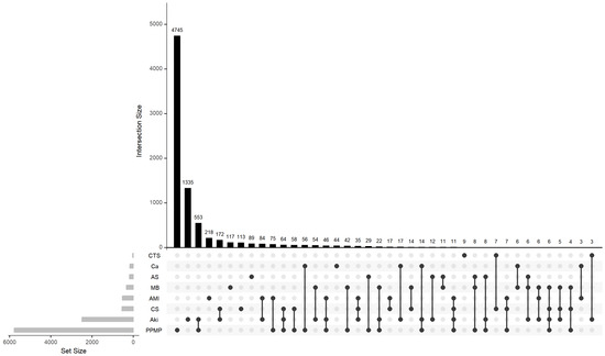
Figure 1.
Upset plot of complications.
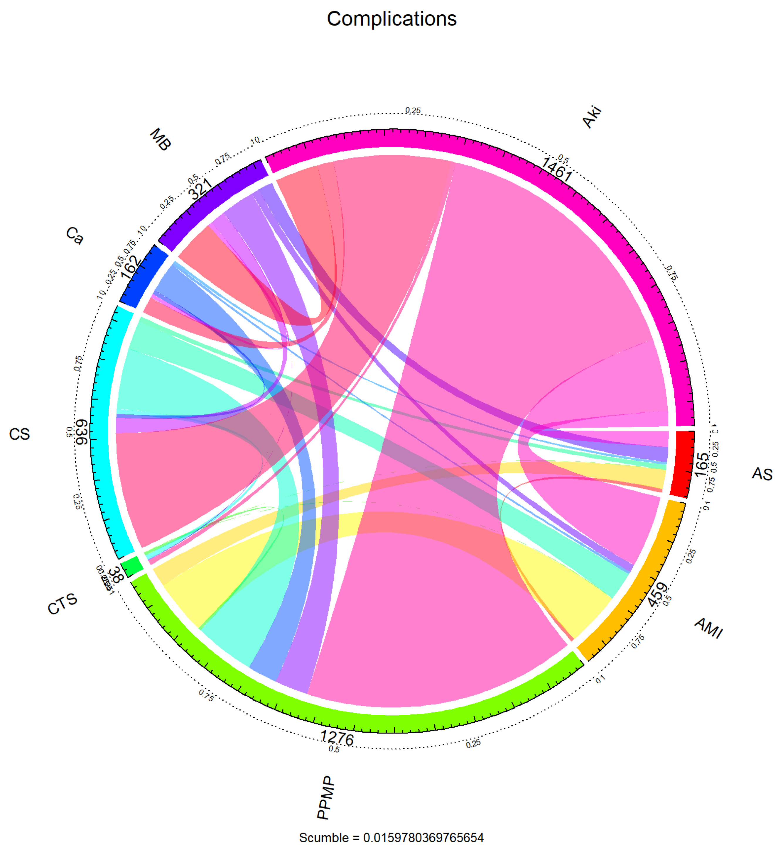
To further reveal the dependency structure between the labels, the co-occurrence relationship between the labels was visualised using a chord diagram in Figure 2. The arcs in the figure represent the marginal frequencies of each tag, and the connected bands reflect the co-occurrence intensity between tags. It can be seen that “PPMP” not only has the highest marginal frequency but also has intensive co-occurrence with multiple labels (e.g., “AKI”, “AMI”, “AS”, etc.), forming a centralised structure, suggesting that these labels may show a strong synergistic seizure pattern in clinical situations. On the other hand, labels such as “CTS” and “Ca” co-occur more in isolation or with only a small number of labels. This label co-occurrence network shows a clear hub-and-spoke pattern, where a small number of core labels are unevenly coupled with a large number of peripheral labels.
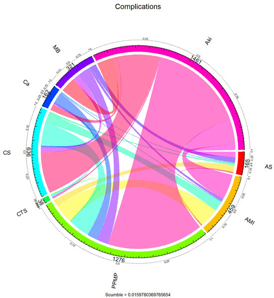
Figure 2.
Chord diagram of complications.
For demographic characteristics of this dataset, 56.16% were males and 43.84% were females. The minimum age of the study population was 2 years, the maximum age was 90 years and the median age was 80 years. The histogram of age distribution is shown in Figure 3, 97.4% of the sample were above 60 years old.
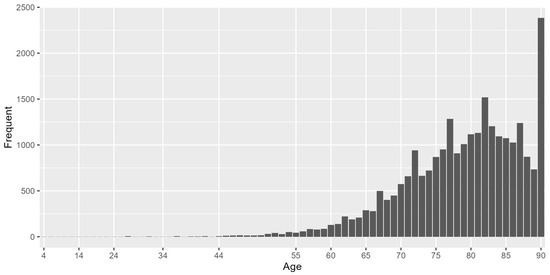
Figure 3.
Histogram of age distribution.
For characteristics of hospitals, we show statistical information on the region where the hospital’s division is located (HOSP_DIVISION) and the hospital’s location and teaching status (HOSP_LOCTEACH). There are nine levels for the region in which the hospital’s division is located, and the region with the highest percentage of location is Middle Atlantic with 17.08%. There were three levels of Hospital Location and Teaching Status, with the largest number of people, 70.2%, treating hospitals in the Urban teaching category. In the subsequent modelling, Rural and Urban nonteaching in HOSP_LOCTEACH were combined into one category to make the distinction between teaching and nonteaching only. Only HOSP_LOCTEACH was included in the analysis in the subsequent modelling.
The levels of independent variables used for modelling analysis are summarised in Table 2:
Table 2.
Independent Variables.
3.2. Model Evaluation Indicators
To assess model effectiveness, a random 70% of the dataset was designated as the training set, and the remaining 30% constituted the validation set. For the above multilabel classification problem, , , , and represent the number of samples that are actually in the positive class and predicted to be in the positive class; the number of samples that are actually in the positive class and incorrectly predicted to be in the negative class; the number of samples that are actually in the negative class and predicted to be in the negative class; and the number of samples that are actually in the negative class and predicted to be the number of samples in which the actual class is negative and the prediction is also negative, respectively.
A series of model evaluation metrics have been proposed for multi-label classification problems, and in this paper, we mainly consider micro-F1, macro-F1, Hamming loss, and micro-AUC. In the multi-label classification task, micro-F1 and macro-F1 are two commonly used variations in the F1-score to measure the overall performance of the model in dealing with the problems of label imbalance and a large number of categories.
Macro F-measure: macro-F1 first calculates the F1 score separately on each labelling dimension and subsequently takes its arithmetic average, thus assigning the same weight to each label. This metric is more sensitive in measuring the model’s performance on all labels and is more effective in revealing the model’s ability to learn on a small number of classes of labels.
where
Micro F-measure: Micro-F1 is an F1 value calculated based on the cumulative result of the confusion matrix at the label level of all samples, and its precision and recall are derived from the overall true positives (TP), false positives (FP) and false negatives (FN) to obtain a unified performance metric. Specifically, micro-F1 emphasises the performance of common labels and is suitable for scenarios with uneven label distribution and large sample size.
where
Hamming loss: It specifies the proportion of labels that are misclassified by the classifier, with lower values indicating better model classification.
where r is the number of samples and b is the number of labels.
Ranking loss: the proportion of non-relevant labels ranked ahead of truly relevant labels, the lower the value, the better the performance of the classifier. The function , in the range [0, 1], gives the probability of relevance of the jth label in the kth test instance. and are the number of relevant and irrelevant labels in that instance, respectively. returns true if p is predicted to be true; otherwise, 0 is returned.
Micro-AUC: it evaluates the proportion of label pairs across all instances where the model assigns a higher score to a relevant label than to an irrelevant one. The higher the value of , the better the performance of the classifier.
3.3. Result Analysis
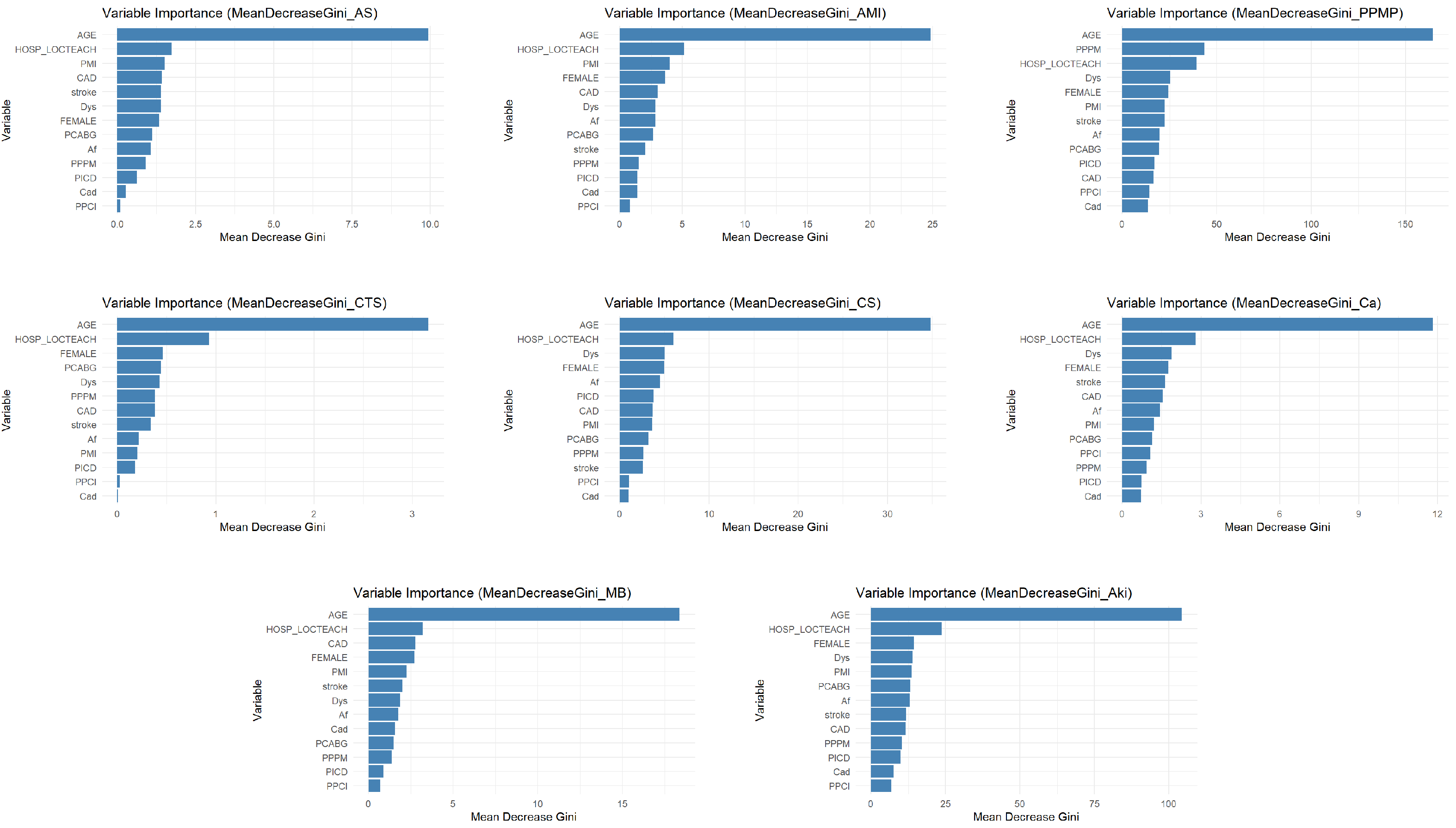
The variable importance analysis, as shown in Figure 4, intuitively reveals that the impact of different comorbidities on specific complications varies significantly. Taking dyslipidemia (Dys) as an example, it exhibits relatively high predictive importance in the placement of PPM (PPMP) and acute kidney injury (Aki), which likely correlates closely with pathophysiological mechanisms such as cardiac dysfunction caused by PPMP and fluid retention and pulmonary edema resulting from Aki. However, Dys’ importance is significantly lower in complications such as acute MI (AMI), conversion to SAVR (CTS) and cancer (Ca), indicating that its predictive value is specific. On the other hand, Implantable Prior ICD (PICD), as an indicator of cardiac interventional therapy, demonstrates some predictive utility for AMI, cardiogenic shock (CS), and Aki. However, its importance is particularly prominent in PPMP. This directly reflects the complexity and severity of cardiovascular diseases in PICD patients, increasing thus their risk of developing other cardiac-related complications. In contrast, the predictive effect of PICD on any stroke/TIA (AS) and CTS is negligible. This refined and differentiated identification of the varying effects of different comorbidities on distinct complications further underscores the necessity of employing shrinkage estimation methods in imbalanced multilabel classification tasks. This approach can precisely capture and quantify these specific associations, leading to the construction of more discriminatory, clinically relevant, and personalized predictive models.
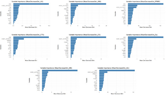
Figure 4.
Variable importance statement.
Before performing multi-label classification, this paper uses five random resampling methods to sample the imbalanced data of this dataset. The results of the data after sampling by the corresponding methods are displayed in Table 3. By comparing the improvement effect of the five preprocessing methods on the imbalance level of the multi-labelled dataset, it is found that LPROS exhibits optimal performance. The experimental data show that the maximum imbalance ratio (MaxIR) is reduced from 507.15 to 40.1 (a relative reduction of 92.1%) and the mean imbalance ratio (MeanIR) is reduced from 92.4 to 13.4 (a reduction of 85.5%) after LPROS processing, which is significantly better than the other methods (LPRUS, MLROS, MLRUS). It is worth noting that LPRUS and MLRUS, based on random undersampling, showed limited improvement in imbalance (MaxIR reduction < 5.5%), while the REMEDIAL method did not change the original data distribution due to its focus on noise processing (% = 0).
Table 3.
Comparison of MaxIR and MeanIR before and after processing.
After sampling the data for multi-label classification, the commonly used representative methods BR, LP, CC, CLR, HOMER, and MLKNN are selected. While those methods are cooperative with the LocalGLMnet-like regularisation part. The corresponding model evaluation metrics are shown in the following tables. In Table 4, Table 5, Table 6, Table 7 and Table 8, the first row, “Original”, indicates results that were not resampled and were derived using the original MLC method.
Table 4.
Hamming loss comparison.
Table 5.
Ranking loss comparison.
Table 6.
Micro F-measure.
Table 7.
Macro F Measure.
Table 8.
Micro AUC.
Table 4 shows the Hamming loss performance of six classifiers (BR, LP, CC, CLR, HOMER, MLKNN) under different resampling methods. The results show that the resampling strategy has a significant effect on the classification performance. Among them, the LPRUS method performs the best and significantly reduces the Hamming loss of multiple classification methods, indicating that it is effective in optimising the sample distribution and improving the classification accuracy. On the contrary, the LPROS method leads to a significant increase in Hamming loss, indicating that it may destroy the original sample structure, thus weakening the model performance. From the perspective of classifiers, CLR and HOMER perform particularly well under LPRUS resampling, but their advantages are not obvious under other sampling strategies; MLKNN is more sensitive to the sampling method, and its performance fluctuates a lot; whereas the performance of BR, LP, and CC is relatively stable under all kinds of sampling strategies; the combination of LPRUS resampling method with CLR or HOMER classifiers can be used as a way of improving the Hamming loss of multi-label classification in this dataset. The LPRUS resampling method combined with CLR or HOMER classifiers can be an effective strategy to improve the performance of Hamming loss for multi-label classification.
Table 5 shows the ranking loss performance. Overall, the LPRUS method achieves the lowest ranking loss among all classifiers, significantly outperforming other resampling strategies, especially on CLR, MLKNN, and HOMER, suggesting that it is effective in optimising the label ranking performance. On the contrary, the LPROS method generally leads to a significant increase in ranking loss, especially in classifiers such as LP and CC, reflecting that it may introduce redundant or misleading samples and destroy the label structure. The overall improvement of the three methods, MLROS, MLRUS, and REMEDIAL, is limited, but REMEDIAL shows some advantages on HOMER and MLKNN, probably due to its ability to optimise label sorting performance. In terms of classifier dimensions, CLR has the best overall performance, with the lowest ranking loss and less sensitivity to sampling strategies; MLKNN responds significantly to sampling methods, and appropriate strategies can bring obvious performance improvement. In summary, LPRUS combined with CLR or MLKNN can be used as a recommended strategy to improve the performance of multi-label classification of this dataset.
Table 6 demonstrates the micro F-measure. The results show that the LPRUS sampling method significantly improves the performance of most of the classification methods, achieving the highest micro F-measure value among several classification methods, demonstrating its effectiveness in optimising the sample distribution and enhancing the model’s classification ability. In contrast, the LPROS sampling method resulted in a general decrease in performance. In terms of classification methods, CLR and HOMER perform optimally under LPRUS sampling, but the advantage is not obvious under other sampling conditions; while BR, LP and CC perform more consistently under different sampling methods, and the performance is affected by sampling in a similar pattern. In summary, LPRUS sampling combined with CLR or HOMER classification methods in this dataset can be used as an effective strategy to improve the performance.
Table 7 reports the macro F-measure results. The overall results show that LPROS is the only resampling method that significantly improves the Macro F values, especially in CC (0.2597), CLR (0.2325), and BR (0.2288) to achieve substantial improvement. For example, the values of BR, LP, CC, CLR and HOMER under this sampling are significantly higher than the other partial sampling cases, which suggests that LPROS sampling is able to optimise the sample distribution to a certain extent and enhance the combined performance of the model in each category. As for LPRUS, MLROS, MLRUS and REMEDIAL sampling methods, the Macro F Measure values of each classification method are generally lower and closer, and the enhancement effect is not obvious. In terms of classification methods, MLKNN performs outstandingly under Original and LPROS sampling, with a Macro F Measure value of 0.4498364, which is much higher than the values of other classification methods under the same sampling, showing that the method is better balanced in predicting each category under specific sampling conditions. On the other hand, BR, LP, CC, CLR, and HOMER have relatively small differences in their performance under different sampling conditions, and the Macro F Measure values are lower in most cases.
Table 8 summarises the micro-AUC results, reflecting the comprehensive discriminative ability of the model on the relevance of sample labels. In terms of overall performance, CLR and MLKNN are the two classifiers with the strongest discriminative ability, obtaining high AUC values under most of the resampling strategies, especially under the LPRUS strategy, MLKNN (0.9242) and CLR (0.9234) achieve the highest micro AUC values. In terms of resampling methods, LPRUS is the only method that improves the AUC in all classifiers, indicating that its optimisation of the sample space structure helps to improve the overall ranking performance of the model, especially for the classifiers such as CLR, MLKNN, CC, etc., MLRUS and MLROS also perform stably and can maintain the AUC values close to or even better than that of the original data in a variety of classifiers with certain generalisation ability. In contrast, the LPROS and REMEDIAL methods fail to improve the AUC performance on most classifiers, and even suffer from significant degradation, suggesting that their resampling strategies may have introduced noise or disturbed the label discrimination boundaries.
It is worth highlighting that CLR is maintained at a high level under all the sampling strategies (minimum 0.8710, maximum 0.9234), showing strong stability and robustness, while MLKNN reaches the optimal value under LPRUS and MLRUS, with strong discriminative performance in the imbalanced label sorting task. In summary, if micro AUC is the main evaluation index, LPRUS is the most effective resampling method, while CLR and MLKNN are the most discriminative multi-label classifiers, and the combination of the two performs particularly well in the multi-label sorting task for this dataset.
Analysis of the provided performance metrics (micro F-measure, macro F-measure, Hamming loss, ranking loss, and micro-AUC) across various resampling and classification methods reveals distinct strengths among the approaches. LPRUS consistently demonstrates superior performance in metrics reflecting overall model accuracy and discrimination, specifically achieving the highest micro F-measure and micro-AUC, alongside the lowest Hamming loss and ranking loss across most classifiers. This indicates its efficacy in enhancing general predictive performance, reducing misclassification rates, and improving ranking quality. Conversely, LPROS excels remarkably in Macro F Measure, showcasing its significant capability to mitigate class imbalance issues and improve the predictive performance for minority classes, albeit at a potential cost of slightly diminished overall accuracy metrics. The performance of MLROS, MLRUS, and REMEDIAL generally falls between these two extremes, offering modest improvements over the “Original” approach but not matching the consistent superiority of LPRUS in aggregate metrics or the specialized strength of LPROS in handling class imbalance. Therefore, the “best” model selection hinges on the specific objectives: LPRUS-based models are optimal for achieving robust overall predictive accuracy and minimizing errors, while LPROS is paramount when prioritizing the accurate identification and recall of rare events or minority classes within imbalanced datasets.
In this study, most models exhibited high computational efficiency during the fitting phase, with the exception of MLkNN-based methods, which were comparatively slower. This indicates that once trained, these models can generate predictions rapidly, making them promising for quick deployment in real-world clinical settings. However, a detailed analysis of prediction latency and specific optimizations for real-time deployment falls beyond the immediate scope of this research.
4. Discussion
In this paper, we constructed an adjustment assessment model for adjusting evidence from randomised clinical trials (RCTs) to real-world data (RWD), introduce a LocalGLMnet-like shrinkage estimation in multi-label classification methods to handle the problem that not all covariates exert an equal influence. Our empirical analysis identified CLR+LPRUS as the optimal model combination for predicting TAVR postoperative complications. This pairing consistently minimised Hamming/ranking loss while maximising micro-F1 and micro-AUC across various multi-label classifiers. Notably, MLKNN+Original also demonstrated superior Macro F1 and micro-AUC, proving effective for addressing label imbalance and niche labels. These findings underscore LPRUS’s general efficacy, contrasting with the limited gains or degradation observed from non-label-aware resampling.
The limitations of this study are primarily reflected in the following five aspects: First, the limitations of handling label imbalance. Despite employing various resampling strategies, while the model’s overall performance (micro F-score) improved, its predictive ability for individual labels (macro F-score) remained unbalanced, which may be attributed to the perturbation of label structure and semantic relationships by resampling methods, as well as the classifier’s insufficient learning capability for low-frequency labels. Second, data quality and volume constraints. The limited overall sample size for TAVR postoperative complications may affect the model’s generalisation ability, particularly leading to high variance in predicting rare complication categories; moreover, the model’s reliance on the accuracy and completeness of ICD coding presents a potential limitation to the reliability of results. Third, insufficient exploration of label correlations. Although chained classifiers were utilised, this study has not yet introduced comparisons with other existing methods for complex label dependency modelling, indicating room for future performance enhancement in this regard. Fourth, the potential for overfitting. Based on the current data and model complexity, the developed model may still present a risk of overfitting. Fifth, the lack of prospective validation. As a retrospective analysis, the model’s generalizability and robustness in real-world clinical settings still require comprehensive evaluation and validation through prospective studies.
The model developed in this study demonstrates significant clinical application potential in TAVR complication prediction, capable of assisting physicians in optimising perioperative management across multiple dimensions. Specifically, the model can be utilised for precise preoperative risk assessment and patient stratification, thereby aiding physicians in making more informed surgical decisions, optimising resource allocation, and facilitating informed consent. Concurrently, the model’s predictive results contribute to guiding personalised intraoperative and postoperative management strategies, enabling early intervention for high-risk patients, which in turn effectively lowers the incidence of complications, improves patient prognosis, and enhances overall medical quality and efficiency. Furthermore, this model can also serve as a tool for medical education and training, deepening medical professionals’ understanding of TAVR complication risk factors. In summary, this model aims to translate data insights into practical clinical actions, ultimately achieving a comprehensive improvement in TAVR patients’ treatment outcomes and quality of life.
Author Contributions
Methodology, Y.X.; Software, Y.Z.; Writing—original draft, Y.Z.; Writing—review & editing, Y.Z.; Supervision, Y.X.; Funding acquisition, Y.X. All authors have read and agreed to the published version of the manuscript.
Funding
This paper is funded by the “Huiyuan Outstanding Young Scholar Project” of the University of International Business and Economics (Project Number: 21JQ07).
Data Availability Statement
The raw data supporting the conclusions of this article will be made available by the authors on request.
Conflicts of Interest
The authors declare no conflicts of interest.
References
- Tsoumakas, G.; Katakis, I.; Vlahavas, I. Random k-labelsets for multilabel classification. IEEE Trans. Knowl. Data Eng. 2010, 23, 1079–1089. [Google Scholar] [CrossRef]
- Charte, F.; Rivera, A.; del Jesus, M.J.; Herrera, F. A first approach to deal with imbalance in multi-label datasets. In Hybrid Artificial Intelligent Systems, Proceedings of the 8th International Conference, HAIS 2013, Salamanca, Spain, 11–13 September 2013; Proceedings 8; Springer: Berlin/Heidelberg, Germany, 2013; pp. 150–160. [Google Scholar]
- Fürnkranz, J.; Hüllermeier, E.; Loza Mencía, E.; Brinker, K. Multilabel classification via calibrated label ranking. Mach. Learn. 2008, 73, 133–153. [Google Scholar] [CrossRef]
- Tsoumakas, G.; Katakis, I.; Vlahavas, I. Mining multi-label data. In Data Mining and Knowledge Discovery Handbook; Springer: Boston, MA, USA, 2010; pp. 667–685. [Google Scholar]
- Boutell, M.R.; Luo, J.; Shen, X.; Brown, C.M. Learning multi-label scene classification. Pattern Recognit. 2004, 37, 1757–1771. [Google Scholar] [CrossRef]
- Read, J.; Pfahringer, B.; Holmes, G.; Frank, E. Classifier chains for multi-label classification. Mach. Learn. 2011, 85, 333–359. [Google Scholar] [CrossRef]
- Tsoumakas, G.; Vlahavas, I. Random k-labelsets: An ensemble method for multilabel classification. In Proceedings of the 18th European Conference on Machine Learning, Warsaw, Poland, 17–21 September 2007; Springer: Berlin/Heidelberg, Germany, 2007; pp. 406–417. [Google Scholar]
- Zhang, M.; Zhou, Z. A k-nearest neighbor based algorithm for multi-label classification. In Proceedings of the 2005 IEEE International Conference on Granular Computing, Beijing, China, 25–27 July 2005; Volume 2, pp. 718–721. [Google Scholar]
- Mencía, E.L.; Furnkranz, J. Pairwise learning of multilabel classifications with perceptrons. In Proceedings of the 2008 IEEE International Joint Conference on Neural Networks (IEEE World Congress on Computational Intelligence), Hong Kong, China, 1–8 June 2008; pp. 2899–2906. [Google Scholar]
- Elisseeff, A.; Weston, J. A kernel method for multi-labelled classification. In Advances in Neural Information Processing Systems 14; MIT Press: Cambridge, MA, USA, 2001. [Google Scholar]
- Tarekegn, A.N.; Giacobini, M.; Michalak, K. A review of methods for imbalanced multi-label classification. Pattern Recognit. 2021, 118, 107965. [Google Scholar] [CrossRef]
- Rivera, A.J.; Dávila, M.A.; Elizondo, D.; del Jesus, M.J.; Charte, F. mldr. resampling: Efficient reference implementations of multilabel resampling algorithms. Neurocomputing 2023, 559, 126806. [Google Scholar] [CrossRef]
- Sun, K.W.; Lee, C.H. Addressing class-imbalance in multi-label learning via two-stage multi-label hypernetwork. Neurocomputing 2017, 266, 375–389. [Google Scholar] [CrossRef]
- Luo, F.-F.; Guo, W.-Z.; Chen, G.L. Addressing imbalance in weakly supervised multi-label learning. IEEE Access 2019, 7, 37463–37472. [Google Scholar] [CrossRef]
- Pouyanfar, S.; Wang, T.; Chen, S.-C. A multi-label multimodal deep learning framework for imbalanced data classification. In Proceedings of the 2019 IEEE Conference on Multimedia Information Processing and Retrieval (MIPR), San Jose, CA, USA, 28–30 March 2019; pp. 199–204. [Google Scholar]
- Wan, S.; Duan, Y.; Zou, Q. Hpslpred: An ensemble multi-label classifier for human protein subcellular location prediction with imbalanced source. Proteomics 2017, 17, 1700262. [Google Scholar] [CrossRef]
- Tahir, M.A.; Kittler, J.; Mikolajczyk, K.; Yan, F. Improving multilabel classification performance by using ensemble of multi-label classifiers. In Multiple Classifier Systems, Proceedings of the 9th International Workshop, MCS 2010, Cairo, Egypt, 7–9 April 2010; Proceedings 9; Springer: Berlin/Heidelberg, Germany, 2010; pp. 11–21. [Google Scholar]
- Sun, Y.; Kamel, M.S.; Wong, A.K.C.; Wang, Y. Cost-sensitive boosting for classification of imbalanced data. Pattern Recognit. 2007, 40, 3358–3378. [Google Scholar] [CrossRef]
- Guo, H.; Li, Y.; Shang, J.; Gu, M.; Huang, Y.; Gong, B. Learning from class-imbalanced data: Review of methods and applications. Expert Syst. Appl. 2017, 73, 220–239. [Google Scholar]
- Liu, X.; Wu, J.; Zhou, Z. Exploratory undersampling for class-imbalance learning. IEEE Trans. Syst. Man Cybern. Part B (Cybern.) 2008, 39, 539–550. [Google Scholar]
- Castellanos, F.J.; Valero-Mas, J.J.; Calvo-Zaragoza, J.; Rico-Juan, J.R. Oversampling imbalanced data in the string space. Pattern Recognit. Lett. 2018, 103, 32–38. [Google Scholar] [CrossRef]
- Charte, F.; Rivera, A.J.; Jesus, M.J.D.; Herrera, F. Addressing imbalance in multilabel classification: Measures and random resampling algorithms. Neurocomputing 2015, 163, 3–16. [Google Scholar] [CrossRef]
- Charte, F.; Rivera, A.J.; del Jesus, M.J.; Herrera, F. Dealing with difficult minority labels in imbalanced mutilabel data sets. Neurocomputing 2019, 326, 39–53. [Google Scholar] [CrossRef]
- Ge, R.; Zhang, R.; Wang, P. Prediction of chronic diseases with multi-label neural network. IEEE Access 2020, 8, 138210–138216. [Google Scholar] [CrossRef]
- Maxwell, A.; Li, R.; Yang, B.; Weng, H.; Ou, A.; Hong, H.; Zhou, Z.; Gong, P.; Zhang, C. Deep learning architectures for multi-label classification of intelligent health risk prediction. BMC Bioinform. 2017, 18, 121–131. [Google Scholar] [CrossRef]
- Li, R.; Liu, W.; Lin, Y.; Zhao, H.; Zhang, C. An ensemble multilabel classification for disease risk prediction. J. Healthc. Eng. 2017, 2017, 8051673. [Google Scholar] [CrossRef]
- Zhou, L.; Zheng, X.; Yang, D.; Wang, Y.; Bai, X.; Ye, X. Application of multi-label classification models for the diagnosis of diabetic complications. BMC Med. Inform. Decis. Mak. 2021, 21, 182. [Google Scholar] [CrossRef]
- Mintz, G.S. A report of the american college of cardiology task force on clinical expert consensus documents. J. Am. Coll. Cardiol. 2001, 37, 1478–1492. [Google Scholar] [CrossRef]
- Richman, R.; Wüthrich, M.V. Localglmnet: Interpretable deep learning for tabular data. Scand. Actuar. J. 2023, 2023, 71–95. [Google Scholar] [CrossRef]
- Richman, R.; Wüthrich, M.V. Lasso regularization within the localglmnet architecture. Adv. Data Anal. Classif. 2023, 17, 951–981. [Google Scholar] [CrossRef]


Disclaimer/Publisher’s Note: The statements, opinions and data contained in all publications are solely those of the individual author(s) and contributor(s) and not of MDPI and/or the editor(s). MDPI and/or the editor(s) disclaim responsibility for any injury to people or property resulting from any ideas, methods, instructions or products referred to in the content. |
© 2025 by the authors. Licensee MDPI, Basel, Switzerland. This article is an open access article distributed under the terms and conditions of the Creative Commons Attribution (CC BY) license (https://creativecommons.org/licenses/by/4.0/).