Suppressing Nonlinear Resonant Vibrations via NINDF Control in Beam Structures

Abstract

In this paper, a unique method for controlling the effects of nonlinear vibrational responses in a cantilever beam system under harmonic excitation is presented. The Nonlinear Integral Negative Derivative Feedback (NINDF) controller is used for this purpose in this study. With this method, the cantilever beam is represented by a three-DOF nonlinear system, and the NINDF controller is represented by a first-order and second-order filter. The authors derive analytical solutions for the autonomous system with the controller by utilising perturbation analysis on the linearised system model. This study aims to reduce vibration amplitudes in a nonlinear dynamic system, specifically when 1:1 internal resonance occurs. The stability of the system is assessed using the Routh–Hurwitz criterion. Moreover, symmetry is present in the frequency–response curves (FRCs) for a variety of parameter values. The results show that, when compared to other controllers, the effectiveness of vibration suppression is directly correlated with the product of the NINDF control signal. The amplitude response of the system is demonstrated, and the analytical solutions are validated through numerical simulations using the fourth-order Runge–Kutta method. The accuracy and reliability of the suggested approach are demonstrated via the significant correlation between the analytical and numerical results.

1. Introduction

A crucial component in contemporary engineering applications is the cantilever beam, a structural element that is free at one end and fixed at the other. This study examines how a cantilever beam deflects and distributes stress along its length under various load scenarios. Cantilever beams’ capacity to support loads without the need for intermediate supports makes them popular in mechanical and building systems. Cantilever beams’ capacity to support loads without the need for intermediate supports makes them popular in mechanical and building systems. Static equilibrium, elasticity, and material qualities all influence how a cantilever beam behaves. The beam’s shear force and bending moment profiles were assessed using both analytical and numerical techniques. According to the experimental results, the free end experiences the most deflection, which is in line with theoretical predictions. Future research could examine the use of composite materials to lower the weight of cantilever structures and increase their load-carrying capability. Respectively, in recent years, railway researchers have focused a lot of attention on the vibration response analysis of a beam sitting on a foundation to depict a railway track model. An exhaustive analysis of early research in this field of study has been presented [1]. Common applications of the cantilever beam through a middle-of-the-road lumped mass within base excitation include robotic manipulators, high-speed equipment, components of simple constructions, and other models [2,3,4]. The massive free vibration sufficiency of a uniform bar per lumped mass was reduced by [5,6]. Refs. [7,8] looked at bifurcations and the stability of a harmonically activated nonlinear oscillator. Ref. [9] used both analytical and numerical methods to measure the bifurcations and stochastic hop of a cantilever bar within a suffering mass through a perturbation procedure. Using the homotopy analysis method, Ref. [10] investigated the asymptotic solutions for the cantilever beam inside a lumped mass. Numerous systems from fluid mechanics, mathematical biology, plasma physics, hydrodynamics, electrochemistry, nanotechnology, signal processing, and other domains can be modelled using partial differential equations and various fractional derivatives [11,12,13]. Ref. [14] decided to use the differential transformation approach to address the problem of free vibration. Ref. [15] created a saturation-based absorber to lessen the vibrations in the model. Together with the system, they establish the excitation frequency to boost the action of the saturation control. Many techniques have been used to reduce flutter and stabilise unstable oscillations in the field of vibration control for self-excited structures. These initiatives cover every control strategy, all of which are meant to improve system performance and stability. Self-excited oscillations, sometimes referred to as self-sustained oscillations or flutter, are a prominent and common phenomenon in a variety of engineering systems and constructions. Even in cases where the driving forces are insignificant, these oscillations are caused by the interplay between the restoring and inertial forces inside the systems [16]. Targeting nonlinear vibrations in an unforced system of the Rayleigh type, Ref. [17] were the first in NSC to regulate self-excited oscillators. Although they noted some oscillation reduction, they did not highlight the resilience of the controller. Ref. [18] looked for self-excited vibrations in NSC without external excitation and discovered that there were not many mitigating effects. Ref. [19] found that NSC destabilised the system at resonance with little damping when applied to a forced self-excited oscillator. Despite this, they noted that, while raising the damping increased stability, it decreased the efficacy of the controller. For the same self-excited structure, ref. [20] investigated time-delayed PPF control as in [19], observing that performance was adversely affected by time delay. They discovered that they could overcome this problem by increasing loop gain. They re-optimized the mechanism and added a preset time delay to reach stable static equilibrium. In the same structure that was examined in [19,20], ref. [21] employed time-delayed IRC to reduce resonant vibrations and stabilise nonlinear oscillations. Their investigation suggested that IRC could stabilise unstable motions and minimise resonant vibrations, while it could not eliminate vibrations totally. Refs. [22,23] looked into using acceleration and velocity feedback control to eliminate undesired vibrations in a self-excited structure of the Rayleigh type. They discovered that, while the closed-loop system’s performance was negatively impacted by time delays, the ideal filter parameters may successfully lessen or suppress vibrations. In order to improve overall performance, they proposed raising the loop gain. Ref. [24] To get the most out of this control system, NIPPF controllers are added to reduce the vibrations of the Hybrid Rayleigh–Van der Pol–Duffing oscillator with $E_a$ = 15,000. In continuation of the work on this system, ref. [25] used the negative derivative feedback (NDF) control approach, which was additionally implemented to achieve effective vibration suppression. This paper presents a thorough analysis of a unique control technique designed to stabilise the system’s low oscillations away from the resonance and eliminate strong oscillations in self-excited structures at resonant conditions. The suggested control approach entails linking the IRC controller with the NDF, one of which is a first-order filter and the other a second-order filter. The main function of the second-order filter is to channel the strong resonant oscillation from the structure to the filter by creating an energy bridge with the structure at the resonant frequency region. The first-order filter’s major purpose is to alter the negative linear damping of the structure to stabilise the unstable non-resonant oscillations and boost the performance of the second-order filter. The perturbation approach is useful to acquire the frequency-response conditions near simultaneous resonance. This framework’s numerical solutions and reaction amplitude are monitored and analysed. The stability study in the worst resonance situation was determined using phase plane methodology and frequency response equations. We used the MATLABR2021a programs to determine stability studies and vibrational graphs. There is a high degree of agreement between the analytical and numerical answers. A comparison of this research with other recent cantilever beam papers is prepared.

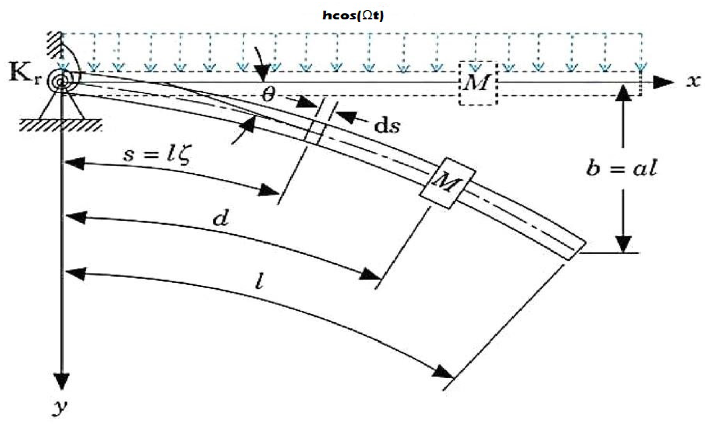
Measured Model

We listed all symbols in

Table 1. List of Symbols.

Notation	Description
$q,\dot{q},\ddot{q}$	Displacement, velocity, and acceleration of the preliminary vein of the system, respectively
$p,\dot{p},\ddot{p}$	Displacement, velocity, and acceleration of the controller, respectively
$z,\dot{z}$	Dimensionless movement and velocity of the controller
${\eta }_1,{\eta }_2$	Dimensionless control signal gain
${\eta }_3,{\eta }_4$	Dimensionless feedback signal gain
${\delta }_2$	Dimensionless linear parameter of the controller
${\alpha }_1,{\alpha }_2$	System and control damping coefficients, respectively
${\omega }_1,{\omega }_2$	The inherent order and patterns in system and control
h	Strength and rate of external forces acting on the system
${\beta }_1,{\gamma }_1,{\delta }_1$	Nonlinear coefficients of the focal structure
$\mathrm{\Omega }$	External excitation frequency
${\sigma }_1,{\sigma }_2$	Detuning parameter
$\epsilon$	Slight variation parameter

.

2. Mathematical Modeling

2.1. Uncontrolled System Dynamics

This section describes the cantilever beam system’s mathematical representation. For this analysis, the structure is simplified and represented as a one-degree-of-freedom system [1], as shown in Figure 1.

$$\ddot{q}+\epsilon {\alpha }_1\dot{q}+\epsilon {\beta }_1{\dot{q}}^3+{\omega }_1^{2}q+\epsilon {\gamma }_1{q}^3+\epsilon {\delta }_1\left(q{\dot{q}}^2+q^2\ddot{q}\right)=\epsilon hcos\left(\mathrm{\Omega }t\right)$$

(1)

2.2. System Dynamics with NINDF Control

Mixed (IRC+NDF) controller design The flowchart of the system integrated with the control unit is shown in Figure 2 with the goal of making clear the order of actions and the dynamic relationships between the different components. The system’s response is analysed under the influence of external forces.

A simplified model, such as the one shown in Figure 1, is frequently used by engineers to analyse the behaviour of cantilever beams. Equations (2)–(4) depict the behaviour of the system in the presence of an external force, taking into account both the external force and the influence of The Nonlinear Integral Negative Derivative Feedback (NINDF). The NINDF may be diligently working to reduce the resulting vibrations.

$$\ddot{q}+\epsilon {\alpha }_1\dot{q}+\epsilon {\beta }_1{\dot{q}}^3+{\omega }_1^{2}q+\epsilon {\gamma }_1{q}^3+\epsilon {\delta }_1\left(q{\dot{q}}^2+q^2\ddot{q}\right)=\epsilon hcos\left(\mathrm{\Omega }t\right)+\epsilon {\eta }_1\dot{p}+\epsilon {\eta }_{2}z$$

(2)

$$\ddot{p}+{\omega }_2^{2}p+\epsilon {\alpha }_2\dot{p}=-\epsilon {\eta }_3\dot{q}$$

(3)

$$\dot{z}+{\delta }_{2}z={\eta }_{4}q$$

(4)

3. Analytical Investigation

3.1. Perturbation Procedure

This section finds an approximate solution for the nonlinear dynamical system using a multiple-time-scale perturbation method (MTSPM). It is possible to derive a first-order approximate solution using this method:

$$q(t;\epsilon )=q_0(T_0,T_1)+\epsilon q_1(T_0,T_1)+O\left({\epsilon }^2\right)$$

(5)

$$p(t;\epsilon )=p_0(T_0,T_1)+\epsilon p_1(T_0,T_1)+O\left({\epsilon }^2\right)$$

(6)

$$z(t;\epsilon )=z_0(T_0,T_1)+\epsilon z_1(T_0,T_1)+O\left({\epsilon }^2\right)$$

(7)

where the insignificant agitation parameter $\epsilon$ is situated at $0<\epsilon \ll 1$ in some location. The agreement specifies two time scales, $T_o$ and $T_1$, where $T_o=t$ denotes a rapid scale, and $T_1=\epsilon t$ denotes a slow one. The time derivatives are converted back into the following:

$${\displaystyle \frac{d}{dt}}=D_0+\epsilon D_1+O\left({\epsilon }^2\right)$$

(8)

$${\displaystyle \frac{d^2}{d{t}^2}}=D_0^2+2\epsilon D_0{D}_1+O\left({\epsilon }^2\right)$$

(9)

Equations (2)–(4) should be modified to include Equations (8) and (9) in order that the following applies:

$$\begin{array}{cc}\hfill & (D_0^2+{\omega }_1^2)q_0+\epsilon (D_0^2+{\omega }_1^2)q_1=\epsilon (hcos\left(\mathrm{\Omega }t\right)+{\eta }_1{D}_0{p}_0+{\eta }_2{z}_0\hfill \\ \hfill & -2D_0{D}_1{q}_0-{\alpha }_1{D}_0{q}_0-{\beta }_1{\left(D_0{q}_0\right)}^3-{\gamma }_1{q}_0^3\hfill \\ \hfill & -{\delta }_1\left(q_0{\left(D_0{q}_0\right)}^2+q_0^2{D}_0^2{q}_0\right))+O\left({\epsilon }^2\right).\hfill \end{array}$$

(10)

$$\begin{array}{cc}\hfill & (D_0^2+{\omega }_2^2)p_0+\epsilon (D_0^2+{\omega }_2^2)p_1=\epsilon \left(-{\eta }_3{D}_0{q}_0-2D_0{D}_1{p}_0-{\alpha }_2{D}_0{p}_0\right)+O\left({\epsilon }^2\right).\hfill \end{array}$$

(11)

$$\begin{array}{cc}\hfill & (D_0+{\delta }_2)z_0+\epsilon (D_0+{\delta }_2)z_1={\eta }_4{q}_0+\epsilon \left({\eta }_4{q}_1-D_1{z}_0\right)+O\left({\epsilon }^2\right).\hfill \end{array}$$

(12)

We now connect the quantities of equal power of $\epsilon$: $O\left({\epsilon }^0\right):$

$$(D_0^2+{\omega }_1^2)q_0=0$$

(13)

$$(D_0^2+{\omega }_2^2)p_0=0$$

(14)

$$(D_0+{\delta }_2)z_0={\eta }_4{q}_0$$

(15)

$O\left({\epsilon }^1\right):$

$$\begin{array}{cc}\hfill (D_0^2+{\omega }_1^2)q_1=& hcos\left(\mathrm{\Omega }t\right)+{\eta }_1{D}_0{p}_0+{\eta }_2{z}_0\hfill \\ \hfill & -2D_0{D}_1{q}_0-{\alpha }_1{D}_0{q}_0-{\beta }_1{\left(D_0{q}_0\right)}^3\hfill \\ \hfill & -{\gamma }_1{q}_0^3-{\delta }_1\left(q_0{\left(D_0{q}_0\right)}^2+q_0^2{D}_0^2{q}_0\right)\hfill \end{array}$$

(16)

$$(D_0^2+{\omega }_2^2)p_1=-{\eta }_3{D}_0{q}_0-2D_0{D}_1{p}_0-{\alpha }_2{D}_0{p}_0$$

(17)

$$(D_0+{\delta }_2)z_1={\eta }_4{q}_1-D_1{z}_0$$

(18)

After solving the standardised differential equations from Equations (13)–(15), we get the following:

$$q_o=A\left(T_1\right)e^{i{\omega }_1{T}_0}+\overline{A}{e}^{-i{\omega }_1{T}_0}$$

(19)

$$p_o=B\left(T_1\right)e^{i{\omega }_2{T}_0}+\overline{B}{e}^{-i{\omega }_2{T}_0}$$

(20)

$$z_o=\left({\displaystyle \frac{{\delta }_2-i{\omega }_1}{{\delta }_2^2+{\omega }_1^2}}\right)\left({\eta }_{4}A\left(T_1\right)e^{i{\omega }_1{T}_O}\right)+\left({\displaystyle \frac{{\delta }_2+i{\omega }_1}{{\delta }_2^2+{\omega }_1^2}}\right)\left({\eta }_4\overline{A}{e}^{-i{\omega }_1{T}_O}\right)+H\left(T_1\right)e^{-{\delta }_2{T}_O}$$

(21)

Differential Equations (19)–(21) with respect to t are submitted in Equations (16)–(18):

$$\begin{array}{cc}\hfill (D_0^2+{\omega }_1^2)q_1& ={\displaystyle \frac{h}{2}}{e}^{i\mathrm{\Omega }{T}_0}+{\eta }_{1}i{\omega }_{2}B{e}^{i{\omega }_2{T}_0}\hfill \\ \hfill & +{\eta }_2\left({\eta }_4{\displaystyle \frac{{\delta }_2-i{\omega }_1}{{\delta }_2^2+{\omega }_1^2}}A{e}^{i{\omega }_1{T}_0}+H\left(T_1\right)e^{-{\delta }_2{T}_0}\right)\hfill \\ \hfill & -2i{\omega }_1{D}_{1}A{e}^{i{\omega }_1{T}_0}\hfill \\ \hfill & +\left[-i{\omega }_1{\alpha }_{1}A-3i{\beta }_1{\omega }_1^3{A}^2\overline{A}-3{\gamma }_1{A}^2\overline{A}+2{\delta }_1{\omega }_1^2{A}^2\overline{A}\right]e^{i{\omega }_1{T}_0}\hfill \\ \hfill & +\left[i{\beta }_1{\omega }_1^3{A}^3-{\gamma }_1{A}^3+2{\delta }_1{\omega }_1^2{A}^3\right]e^{3i{\omega }_1{T}_0}\hfill \\ \hfill & +\mathrm{C}.\mathrm{C}.\hfill \end{array}$$

(22)

$$(D_0^2+{\omega }_2^2)p_1=-{\eta }_{3}i{\omega }_{1}A{e}^{i{\omega }_1{T}_0}-2i{\omega }_2{D}_{1}B{e}^{i{\omega }_2{T}_0}-{\alpha }_{2}i{\omega }_{2}B{e}^{i{\omega }_2{T}_0}+\mathrm{C}.\mathrm{C}.$$

(23)

After secular terms are eliminated, $q_1$, $p_1$, and $z_1$ take the following forms:

$$q_1=H_1{e}^{3i{\omega }_1{T}_O}+H_2{e}^{i{\omega }_2{T}_O}+H_3{e}^{i\mathrm{\Omega }{T}_O}+\mathrm{C}.\mathrm{C}.,$$

(24)

$$p_1=H_4{e}^{i{\omega }_1{T}_O}+\mathrm{C}.\mathrm{C}.$$

(25)

$$z_1=H_5{e}^{3i{\omega }_1{T}_O}+H_6{e}^{i{\omega }_2{T}_O}+H_7{e}^{i\mathrm{\Omega }{T}_O}+H_8{e}^{(i{\omega }_1-{\delta }_2)T_O}+[K-T_0{D}_{1}H]e^{-{\delta }_2{T}_O}+\mathrm{C}.\mathrm{C}.,$$

(26)

where $H_i$ for $i=1,2,\dots ,8$ are provided in Appendix A. Under the abbreviation C. C., the complex conjugate components are collected. The following versions can be obtained by eliminating the secular terms:

$$\begin{array}{cc}\hfill 2i{\omega }_1{D}_{1}A{e}^{i{\omega }_1{T}_O}& ={\displaystyle \frac{h}{2}}{e}^{i\mathrm{\Omega }{T}_O}+{\eta }_{1}i{\omega }_{2}B{e}^{i{\omega }_2{T}_O}\hfill \\ \hfill & +{\eta }_2{\eta }_4\left({\displaystyle \frac{{\delta }_2-i{\omega }_1}{{\delta }_2^2+{\omega }_1^2}}\right)A{e}^{i{\omega }_1{T}_O}\hfill \\ \hfill & +\left[-i{\omega }_{1}A{\alpha }_1-3i{\beta }_1{\omega }_1^3{A}^2\overline{A}-3{\gamma }_1{A}^2\overline{A}+2{\delta }_1{\omega }_1^2{A}^2\overline{A}\right]e^{i{\omega }_1{T}_O}\hfill \end{array}$$

(27)

$$\begin{array}{c}\hfill 2i{\omega }_2{D}_{1}B{e}^{i{\omega }_2{T}_O}=-i{\alpha }_2{\omega }_{2}B{e}^{i{\omega }_2{T}_O}-i{\eta }_3{\omega }_{1}A{e}^{i{\omega }_1{T}_O}\end{array}$$

(28)

We inferred the following resonances using the first approximation:

(i)

Primary resonance case (PR): $\mathrm{\Omega }={\omega }_1$.

(ii)

Internal resonance case (IR): ${\omega }_1={\omega }_2$.

(iii)

Simultaneous resonance (PR) and (IR) resonance: $\mathrm{\Omega }={\omega }_1={\omega }_2$. (The worst case.)

3.2. Periodic Solutions

Using the second hand to confer the solvability surroundings, we will familiarise the detuning parameters ${\sigma }_1$ and ${\sigma }_2$ for the selected resonance cases $\mathrm{\Omega }={\omega }_1$ and ${\omega }_1={\omega }_2$ so that the following applies:

$$\mathrm{\Omega }={\omega }_1+\epsilon {\sigma }_1$$

(29)

$${\omega }_2={\omega }_1+\epsilon {\sigma }_2$$

(30)

The solvability criteria can be compiled as follows by including Equations (29) and (30) in the secular and negligible division terms in Equations (27) and (28):

$$\begin{array}{cc}\hfill 2i{\omega }_1{D}_{1}A=& {\displaystyle \frac{h}{2}}{e}^{i{\sigma }_1{T}_1}+i{\eta }_1{\omega }_{2}B{e}^{i{\sigma }_2{T}_1}+{\eta }_2{\eta }_4\left({\displaystyle \frac{{\delta }_2-i{\omega }_1}{{\delta }_2^2+{\omega }_1^2}}\right)A\hfill \\ \hfill & -i{\omega }_{1}A{\alpha }_1-3i{\beta }_1{\omega }_1^3{A}^2\overline{A}-3{\gamma }_1{A}^2\overline{A}+2{\delta }_1{\omega }_1^2{A}^2\overline{A}\hfill \end{array}$$

(31)

$$2i{\omega }_2{D}_{1}B=-i{\alpha }_2{\omega }_{2}B-i{\eta }_3{\omega }_{1}A{e}^{-i{\sigma }_2{T}_1}$$

(32)

Exchange A and B using the polar form as follows to investigate the resolution of (31) and (32):

$$A\left(T_1\right)={\displaystyle \frac{1}{2}}{a}_1\left(T_1\right)e^{i{\theta }_1{T}_1},D_{1}A={\displaystyle \frac{1}{2}}\left({\dot{a}}_1+i{a}_1{\dot{\theta }}_1\right)e^{i{\theta }_1{T}_1}.$$

(33)

$$B\left(T_1\right)={\displaystyle \frac{1}{2}}{a}_2\left(T_1\right)e^{i{\theta }_2{T}_1},D_{1}B={\displaystyle \frac{1}{2}}\left({\dot{a}}_2+i{a}_2{\dot{\theta }}_2\right)e^{i{\theta }_2{T}_1}.$$

(34)

where ${\varphi }_1$ and ${\varphi }_2$ are expressed as the motion’s phases, and $a_1$ and $a_2$ are the system’s and control motion’s steady-state amplitudes, respectively. When (33) and (34) are inserted into (31) and (32), the amplitude-phase modifying equations that result are as follows:

$${\dot{a}}_1=-{\displaystyle \frac{1}{2}}{a}_1{\alpha }_1-{\displaystyle \frac{a_1{\eta }_2{\eta }_4}{2({\delta }_2^2+{\omega }_1^2)}}+{\displaystyle \frac{h}{2{\omega }_1}}sin{\varphi }_1+{\displaystyle \frac{a_2{\eta }_1{\omega }_2}{2{\omega }_1}}cos{\varphi }_2-{\displaystyle \frac{3{\beta }_1{a}_1^3{\omega }_1^2}{8}}$$

(35)

$$a_1{\dot{\theta }}_1={\displaystyle \frac{3{\gamma }_1{a}_1^3}{8{\omega }_1}}-{\displaystyle \frac{{\delta }_1{\omega }_1{a}_1^3}{4}}-{\displaystyle \frac{a_1{\eta }_2{\eta }_4{\delta }_2}{2{\omega }_1({\delta }_2^2+{\omega }_1^2)}}-{\displaystyle \frac{h}{2{\omega }_1}}cos{\varphi }_1+{\displaystyle \frac{a_2{\eta }_1{\omega }_2}{2{\omega }_1}}sin{\varphi }_2$$

(36)

$${\dot{a}}_2=-{\displaystyle \frac{1}{2}}{a}_2{\alpha }_2-{\displaystyle \frac{a_1{\eta }_3{\omega }_1}{2{\omega }_2}}cos{\varphi }_2$$

(37)

$$a_2{\dot{\theta }}_2={\displaystyle \frac{a_1{\eta }_3{\omega }_1}{2{\omega }_2}}sin{\varphi }_2$$

(38)

As ${\varphi }_1={\sigma }_1{T}_1-{\theta }_1$ and ${\varphi }_2={\sigma }_2{T}_1+{\theta }_2-{\theta }_1$, respectively. With reference to the main system parameters, the following equations are present:

$${\dot{a}}_1=-{\displaystyle \frac{1}{2}}{a}_1{\alpha }_1-{\displaystyle \frac{a_1{\eta }_2{\eta }_4}{2({\delta }_2^2+{\omega }_1^2)}}+{\displaystyle \frac{h}{2{\omega }_1}}sin{\varphi }_1+{\displaystyle \frac{a_2{\eta }_1{\omega }_2}{2{\omega }_1}}cos{\varphi }_2-{\displaystyle \frac{3{\beta }_1{a}_1^2{\omega }_1^2}{8}}$$

(39)

$${\dot{\varphi }}_1={\sigma }_1-{\displaystyle \frac{3{\gamma }_1{a}_1^2}{8{\omega }_1}}+{\displaystyle \frac{{\delta }_1{\omega }_1{a}_1^2}{4}}+{\displaystyle \frac{{\eta }_2{\eta }_4{\delta }_2}{2{\omega }_1({\delta }_2^2+{\omega }_1^2)}}+{\displaystyle \frac{h}{2a_1{\omega }_1}}cos{\varphi }_1-{\displaystyle \frac{a_2{\eta }_1{\omega }_2}{2a_1{\omega }_1}}sin{\varphi }_2$$

(40)

$${\dot{a}}_2=-{\displaystyle \frac{1}{2}}{a}_2{\alpha }_2-{\displaystyle \frac{a_1{\eta }_3{\omega }_1}{2{\omega }_2}}cos{\varphi }_2$$

(41)

$${\dot{\varphi }}_2=({\sigma }_2-{\sigma }_1)+{\dot{\varphi }}_1+{\displaystyle \frac{a_1{\eta }_3{\omega }_1}{2a_2{\omega }_2}}sin{\varphi }_2$$

(42)

The efficiency of the control rule will be evaluated by calculating the equilibrium solutions of Equations (39)–(42) and examining their firmness as a function of the parameters $({\sigma }_1,{\sigma }_2,{\eta }_i(i=1,2,3,4),{\delta }_1,{\delta }_2,h,{\gamma }_1, \mathrm{and}{\beta }_1)$.

3.3. Fixed-Point Solution

A steady-state solution to Equations (39)–(42) may have a fixed point, which may be obtained by stroking ${\dot{a}}_1={\dot{a}}_2={\dot{\varphi }}_1={\dot{\varphi }}_2=0$.

$${\displaystyle \frac{h}{2{\omega }_1}}sin{\varphi }_1+{\displaystyle \frac{a_2{\eta }_1{\omega }_2}{2{\omega }_1}}cos{\varphi }_2={\displaystyle \frac{1}{2}}{a}_1{\alpha }_1+{\displaystyle \frac{a_1{\eta }_2{\eta }_4}{2({\delta }_2^2+{\omega }_1^2)}}+{\displaystyle \frac{3{\beta }_1{a}_1^3{\omega }_1^2}{8}}$$

(43)

$${\displaystyle \frac{h}{2{\omega }_1}}cos{\varphi }_1-{\displaystyle \frac{a_2{\eta }_1{\omega }_2}{2{\omega }_1}}sin{\varphi }_2=-a_1{\sigma }_1+{\displaystyle \frac{3{\gamma }_1{a}_1^3}{8{\omega }_1}}-{\displaystyle \frac{{\delta }_1{\omega }_1{a}_1^3}{4}}-{\displaystyle \frac{a_1{\eta }_2{\eta }_4{\delta }_2}{2{\omega }_1({\delta }_2^2+{\omega }_1^2)}}$$

(44)

$${\displaystyle \frac{a_1{\eta }_3{\omega }_1}{2{\omega }_2}}cos{\varphi }_2=-{\displaystyle \frac{1}{2}}{a}_2{\alpha }_2$$

(45)

$${\displaystyle \frac{a_1{\eta }_3{\omega }_1}{2{\omega }_2}}sin{\varphi }_2=a_2({\sigma }_1-{\sigma }_2)$$

(46)

To get the following equation, square Equations (45) and (46), and then add their two sides:

$$[4{\omega }_2^2{({\sigma }_1-{\sigma }_2)}^2+{\alpha }_2^2{\omega }_2^2]a_2^2=\left({\eta }_3^2{\omega }_1^2\right)a_1^2$$

(47)

From Equations (45) and (46), we have:

$$cos{\varphi }_2=-{\displaystyle \frac{{\omega }_2{a}_2{\alpha }_2}{{\eta }_3{\omega }_1{a}_1}}$$

(48)

$$sin{\varphi }_2={\displaystyle \frac{2{\omega }_2({\sigma }_1-{\sigma }_2)a_2}{{\eta }_3{\omega }_1{a}_1}}$$

(49)

Inserting (48) and (49) into (43) and (44), we obtain the following:

$$sin{\varphi }_1={\displaystyle \frac{2{\omega }_1}{h}}\left[{\displaystyle \frac{1}{2}}{a}_1{\alpha }_1+{\displaystyle \frac{a_1{\eta }_2{\eta }_4}{2({\delta }_2^2+{\omega }_1^2)}}+{\displaystyle \frac{{\eta }_1{\omega }_2^2{\alpha }_2{a}_2^2}{2{\eta }_3{\omega }_1^2{a}_1}}+{\displaystyle \frac{3{\beta }_1{a}_1^3{\omega }_1^2}{8}}\right]$$

(50)

$$cos{\varphi }_1={\displaystyle \frac{2{\omega }_1}{h}}\left[-a_1{\sigma }_1+{\displaystyle \frac{3{\gamma }_1{a}_1^3}{8{\omega }_1}}-{\displaystyle \frac{{\delta }_1{\omega }_1{a}_1^3}{4}}-{\displaystyle \frac{a_1{\eta }_2{\eta }_4{\delta }_2}{2{\omega }_1({\delta }_2^2+{\omega }_1^2)}}+{\displaystyle \frac{{\eta }_1{\omega }_2^2({\sigma }_1-{\sigma }_2)a_2^2}{{\eta }_3{\omega }_1^2{a}_1}}\right]$$

(51)

Squaring and adding Equations (50) and (51), we obtain the following:

$$\begin{array}{c}\hfill {\left({\displaystyle \frac{1}{2}}{a}_1{\alpha }_1+{\displaystyle \frac{a_1{\eta }_2{\eta }_4}{2({\delta }_2^2+{\omega }_1^2)}}+{\displaystyle \frac{{\eta }_1{\omega }_2^2{\alpha }_2{a}_2^2}{2{\eta }_3{\omega }_1^2{a}_1}}+{\displaystyle \frac{3{\beta }_1{a}_1^3{\omega }_1^2}{8}}\right)}^2\\ \hfill +{\left({\displaystyle \frac{3{\gamma }_1{a}_1^3}{8{\omega }_1}}-a_1{\sigma }_1-{\displaystyle \frac{{\delta }_1{\omega }_1{a}_1^3}{4}}-{\displaystyle \frac{a_1{\eta }_2{\eta }_4{\delta }_2}{2{\omega }_1({\delta }_2^2+{\omega }_1^2)}}+{\displaystyle \frac{{\eta }_1{\omega }_2^2({\sigma }_1-{\sigma }_2)a_2^2}{{\eta }_3{\omega }_1^2{a}_1}}\right)}^2\\ \hfill ={\displaystyle \frac{h^2}{4{\omega }_1^2}}\end{array}$$

(52)

In the reasonable situation ($a_1\ne 0,a_2\ne 0$), the behaviour of the system’s steady-state solutions is described by the frequency response Equations (39) and (42).

3.4. Gaining Stability Through System Linearisation

We examined the Jacobian matrix’s eigenvalues, which were obtained from the equations’ right-hand side, to ascertain the equilibrium solution’s stability. An equilibrium solution is said to be asymptotically stable if every eigenvalue has negative real components. In contrast, we have some doubts if the eigenvalue has a positive actual part, and the accompanying equilibrium is out of balance. To evolve the stability of the steady-state solution, start by taking these actions. We basically examine the behaviour of minor departures from the steady-state solutions $a_{10},a_{20},{\varphi }_{10},{\varphi }_{20}$ in order to derive the stability principles. Consequently, we embrace the fact that

$$\begin{array}{cc}\hfill a_1& =a_{11}+a_{10},a_2=a_{21}+a_{20},\hfill \\ \hfill {\varphi }_1& ={\varphi }_{11}+{\varphi }_{10},{\varphi }_2={\varphi }_{21}+{\varphi }_{20},\hfill \\ \hfill {\dot{a}}_1& ={\dot{a}}_{11},{\dot{a}}_2={\dot{a}}_{21},\hfill \\ \hfill {\dot{\varphi }}_1& ={\dot{\varphi }}_{11},{\dot{\varphi }}_2={\dot{\varphi }}_{21}.\hfill \end{array}$$

(53)

where $a_{10},a_{20},{\varphi }_{10}, \mathrm{and}{\varphi }_{20}$ fulfil (39) and (42), and $a_{11},a_{21},{\varphi }_{11}, \mathrm{and}{\varphi }_{21}$ are perturbations that should be somehow connected to $a_{10},a_{20},{\varphi }_{10}, \mathrm{and}{\varphi }_{20}$. After resolving (53) into (39)–(42), expanding for small $a_{11},a_{21},{\varphi }_{11}, \mathrm{and}{\varphi }_{21}$, and retaining only the linear terms in $a_{11},a_{21},{\varphi }_{11}, \mathrm{and}{\varphi }_{21}$, we get the following:

$${\dot{a}}_{11}=r_{11}{a}_{11}+r_{12}{\varphi }_{11}+r_{13}{a}_{21}+r_{14}{\varphi }_{21}$$

(54)

$${\dot{\varphi }}_{11}=r_{21}{a}_{11}+r_{22}{\varphi }_{11}+r_{23}{a}_{21}+r_{24}{\varphi }_{21}$$

(55)

$${\dot{a}}_{21}=r_{31}{a}_{11}+r_{32}{\varphi }_{11}+r_{33}{a}_{21}+r_{34}{\varphi }_{21}$$

(56)

$${\dot{\varphi }}_{21}=r_{41}{a}_{11}+r_{42}{\varphi }_{11}+r_{43}{a}_{21}+r_{44}{\varphi }_{21}$$

(57)

The values $r_{ij},i=1,2,3,4\mathrm{and}j=1,2,3,4$ are provided in Appendix A. Equations (54)–(57) can be presented in the resulting matrix:

$${\left[\begin{array}{cccc}{\dot{a}}_{11}& {\dot{\varphi }}_{11}& {\dot{a}}_{21}& {\dot{\varphi }}_{21}\end{array}\right]}^T=\left[\begin{array}{c}J\end{array}\right]{\left[\begin{array}{cccc}{a}_{11}& {\varphi }_{11}& a_{21}& {\varphi }_{21}\end{array}\right]}^T$$

(58)

$$\left[\begin{array}{c}J\end{array}\right]=\left[\begin{array}{cccc}{r}_{11}& r_{12}& r_{13}& r_{14}\\ r_{21}& r_{22}& r_{23}& r_{24}\\ r_{31}& r_{32}& r_{33}& r_{34}\\ r_{41}& r_{42}& r_{43}& r_{44}\end{array}\right]$$

(59)

where $\left[\begin{array}{c}J\end{array}\right]$ is the Jacobian matrix. The stability of the steady-state solutions is controlled via the Jacobian matrix’s eigenvalues. This results in the eigenvalue equation as follows:

$$\left|\begin{array}{cccc}{r}_{11}-\lambda & r_{12}& r_{13}& r_{14}\\ r_{21}& r_{22}-\lambda & r_{23}& r_{24}\\ r_{31}& r_{32}& r_{33}-\lambda & r_{34}\\ r_{41}& r_{42}& r_{43}& r_{44}-\lambda \end{array}\right|=0$$

(60)

At whatever location, the roots of the following polynomial are as follows:

$${\lambda }^4+{\xi }_1{\lambda }^3+{\xi }_2{\lambda }^2+{\xi }_3\lambda +{\xi }_4=0$$

(61)

Equation (59) and $({\xi }_i;i=1,2,3,4)$ have their coefficients labelled in Appendix A. The resolution to the aforementioned system can effectively satisfy the Routh–Hurwitz criterion, which means that the following applies:

$${\xi }_1>0,{\xi }_1{\xi }_2-{\xi }_3>0,{\xi }_3({\xi }_1{\xi }_2-{\xi }_3)-{\xi }_1^2{\xi }_4>0,{\xi }_4>0$$

(62)

4. Results

4.1. Performance of the System Both with and Without NINDF Control

The fourth-order Runge–Kutta process (ode45 in MATLAB) [26] is practical in creating the numerical solution of the specific non-control system in Equations (2)–(4) in order to examine the dynamical system’s performance. The results are displayed graphically as plots of steady-state amplitudes vs. detuning parameters, with figures produced based on the system parameters’ provided values.

$$\begin{array}{c}({\alpha }_1=0.004,{\beta }_1=0.333,{\omega }_1={\omega }_2=\mathrm{\Omega }=1,{\gamma }_1=0.3333,{\delta }_1=3.27455,h=0.07,\hfill \\ {\delta }_2=2.21,{\alpha }_2=0.001,{\eta }_1={\eta }_2={\eta }_3={\eta }_4=1.)\hfill \end{array}$$

The uncontrolled system’s response is depicted in Figure 3 with different values of the force amplitude h, and that clearly indicates that increasing the value of h significantly deteriorates the system’s performance, potentially leading to its failure. In the closed-loop circumstance, the original system’s amplitude was lowered by around 99.99% from its uncontrolled value, as shown in Figure 4, Figure 5 and Figure 6. The fundamental system steady-state amplitudes, which are shown in Figure 4, Figure 5 and Figure 6, where NINDF controllers were previously added at the worst resonance condition, or roughly 0.36. Following the addition of NINDF controllers, the system amplitudes have shrunk by 0.00003 (m). This shows that the NINDF controller’s efficiency ($E_a$), where $E_a$ is equal to the amplitude of the uncontrolled system divided by the amplitude of the controlled system, is roughly 12,000.

4.2. Outcomes and Conversation

This part showed every curve that existed in the model under consideration both before and after a new controller was added. Numerical and graphical solutions are obtained for Equations (39)–(42) in order to obtain the system solution and the NINDF amplitudes. With regard to the detuning parameters ${\sigma }_1$ and ${\sigma }_2$, this graphical solution is generated; two peaks are utilised to show how the amplitudes of these systems change when the detuning parameters ${\sigma }_1$ and ${\sigma }_2$ change. The frequency–response curves’ amplitudes can occasionally be asymmetrical, as shown in Figure 7, Figure 8, Figure 9, Figure 10, Figure 11, Figure 12, Figure 13, Figure 14, Figure 15, Figure 16 and Figure 17. Nonetheless, the symmetry can be enhanced by changing the values of certain variables.

5. Discussion

Figure 7 shows the focal structure and the NINDF controller’s appearances through frequency–response curves. As a function of the detuning parameter ${\sigma }_1$, Figure 7a,b show the steady-state amplitudes of the perpendicular displacement of the main system and the NINDF controller, $a_1$ and $a_2$. This figure indicates that the NINDF controller is helpful in suppressing the vibrations as the resonance cases are shown by the main system amplitude’s minimal value occurring at ${\sigma }_1=0$. As seen in Figure 8a,b, the amplitudes of both the NINDF controller and the main system increase as the external force h increases. As the value of the force h increases, the system’s performance deteriorates, eventually leading to its failure, as previously discussed. Figure 9a,b and Figure 10a,b show that the amplitudes of the system and the controller are minimal for large values of ${\alpha }_1$ and ${\alpha }_2$. Additionally, as illustrated in Figure 11a,b, the amplitudes of the system and the NINDF controller decrease for large values of the natural frequencies ${\omega }_1$ and ${\omega }_2$. We selected three different values for the internal detuning parameter ${\sigma }_2$ in Figure 12. Figure 12a illustrates how the maxima of the main system amplitudes moved to the right as ${\sigma }_2$ increased. As seen in Figure 12b, the left-hand controller peak rises when ${\sigma }_2$ is negative, while the right-hand controller peak rises when ${\sigma }_2$ is positive. These charts show that the basic system amplitude has its minimum value at ${\sigma }_2=-0.1$, ${\sigma }_2=0$, and ${\sigma }_2=0.1$. Figure 13 shows that the vibration discount frequency shifts to the right while retaining symmetry, as seen in Figure 13a, when the efficiency of the linear parameter ${\delta }_2$ increases. Figure 14a,b shows ${\eta }_1$, the control signal gain. We present a collection of conclusions and observations about how the NINDF controller and its parameters affect the performance of the structure. The bandwidth, defined as the distance between the two peaks, represents the frequency range over which the control signal operates. The broader bandwidth observed in the Control NINDF system indicates enhanced dynamic performance and a notable absence of vibrations, as demonstrated in Figure 14a. In accordance with the intended goal of the control signal gain, Figure 14b illustrates that the NINDF controller’s occupancy decreases gradually. In Figure 15a,b, the focal structure amplitude and matching controller amplitude decrease as the control signal gain ${\eta }_2$ is raised. As the feedback signal gain ${\eta }_3$ increases in Figure 16a,b, the vibration suppression bandwidth for the curves simulating the focal structure’s amplitude and the related controller around ${\sigma }_2=0$ also increases, while the system’s amplitude is reduced (Figure 16a), and the controller’s amplitude is increased (Figure 16b). The feedback signal gain ${\eta }_4$’s effect on the controller’s and the focal structure’s frequency–response curves is seen in Figure 17a,b. Increasing the reaction signal reduces the vibration-lessening behaviour in Figure 17a. In Figure 17b, lower controller amplitudes are the result of advanced levels of the feedback signal ${\eta }_4$.

6. Comparison

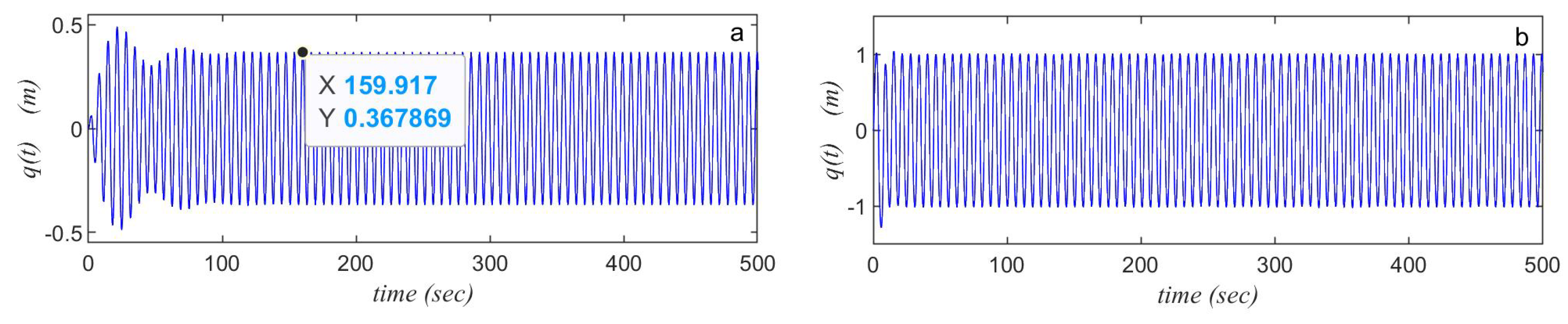
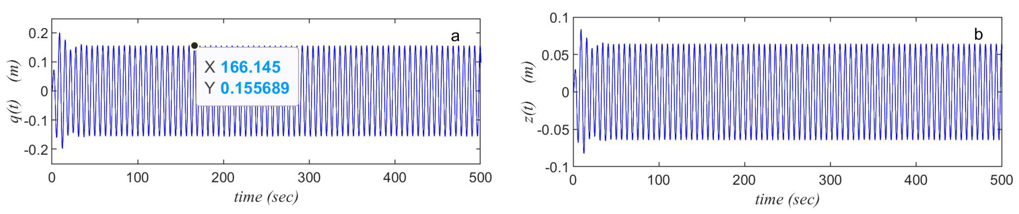
6.1. Comparison Between Time History Before and After Controllers

According to Figure 18, the NINDF controller is the most efficient approach for lessening the amplitude of the focal structure. Additionally, we highlight the strong correspondence between the estimated resolutions and geometric recreations for the unrestrained structure and the structure with the NINDF supervisor.

6.2. Comparison Between Perturbation Solution and Numerical Simulation

Figure 19 shows a comparison between the numerical solution of Equations (2)–(4) and the approximate solution for the full set of Equations (39)–(42) using the many scales technique. Using the fourth-order Runge–Kutta method, the continuous lines display the time histories of the closed loop, while the dashed lines show the approximate solution. It is found that the numerical solution and all of the assumptions made by the approximate solutions accord fairly well.

6.3. Comparison with Previous Work

The current endeavour examines and tracks the authors’ progress in recent publications, as noted in [27]. The behaviour of the cantilever system with mixed controllers (IRC+NSC effect) under various resonance scenarios (simultaneous condition $\mathrm{\Omega }={\omega }_1=2{\omega }_2$) was examined by the authors. Additionally, the same system was controlled by the authors [28] using a variety of controller types; they found that PPF was the most effective and that the controllers decreased the system’s large vibrations under PR+IR resonances with ($E_a=250$). Furthermore, a novel controller (IRC + NDF) for the cantilever beam is examined in this article. Using the new controller on the vibrational structure system and the modified system, we apply several control strategies. In the simultaneous resonance situation ($\mathrm{\Omega }={\omega }_1={\omega }_2$), the results of this work seem to abolish the system’s high vibrational amplitude under harmonic excitation at the highest control impact level, the capacity reached ($E_a$ = 12,000).

7. Conclusions

In this article, the problem of managing nonlinear vibrations in a cantilever beam system has been discussed. The authors have presented a novel method for reducing the lateral vibrations in the system by utilising the NINDF controller. Two second-order nonlinear differential equations were combined with first-order linear differential equations to constitute the mathematical model, which includes the controller and the system. For this nonlinear model, the study used asymptotic analysis to obtain an approximate solution. Frequency response graphs were produced, and the impact of different system and controller circumstances was investigated through an in-depth sensitivity analysis. To evaluate the system’s stability, the Routh–Hurwitz criterion was applied. The analytical results were validated through numerical simulations, which also verify that the frequency response curves are accurate. The frequency response curves’ amplitudes showed improved symmetry when the majority of the parameters were changed. The following succinctly describes the key ideas from the previous discussion:

• In nonlinear structures, high-amplitude atmospheres are successfully reduced via the Nonlinear Integral Negative Derivative Feedback (NINDF) controller.
• Among the worst circumstances of vibrating reverberation are the PR and IR instances $\mathrm{\Omega }={\omega }_1$ and ${\omega }_2={\omega }_1$.
• Following the use of the NINDF reaction supervisor linked to its rate deprived of the regulator, the exciting structure’s breadth decreased by almost 99. 99%.
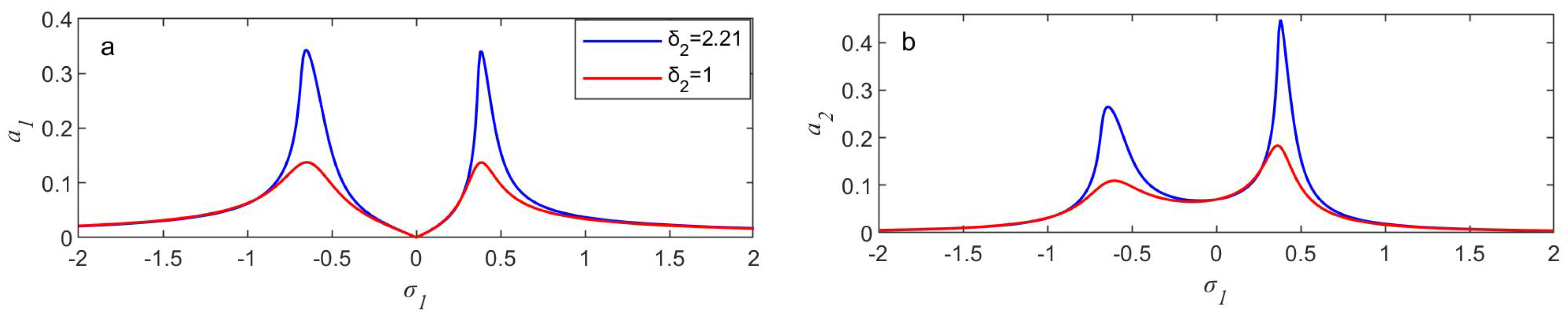
• The NINDF reaction supervisor’s efficiency, represented by $E_a$, influences roughly 12,000, demonstrating how well it supervises the structure’s operation.
• With an increase in the peripheral excitation force, h, the measured structure’s performance or comeback intensifies.
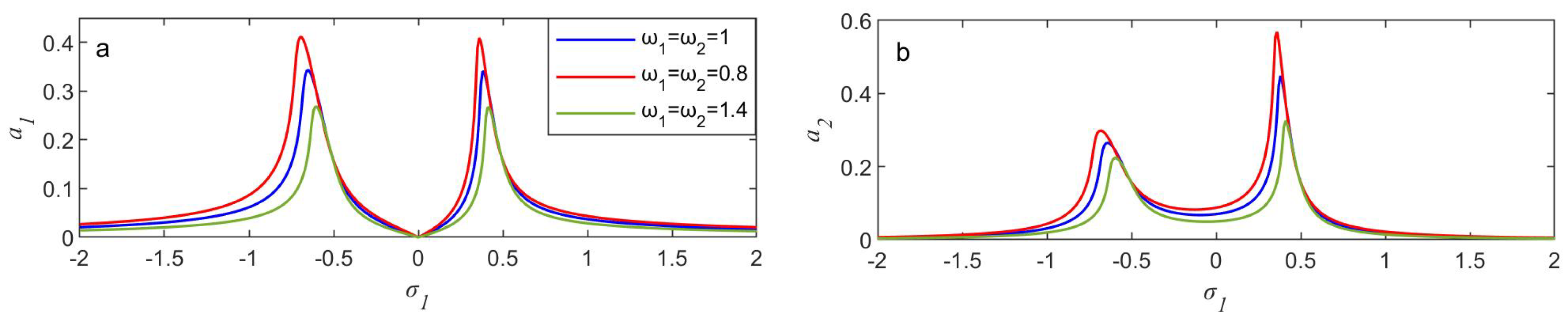
• As the natural frequency ${\omega }_1$ increased, the focal structure’s response dropped.
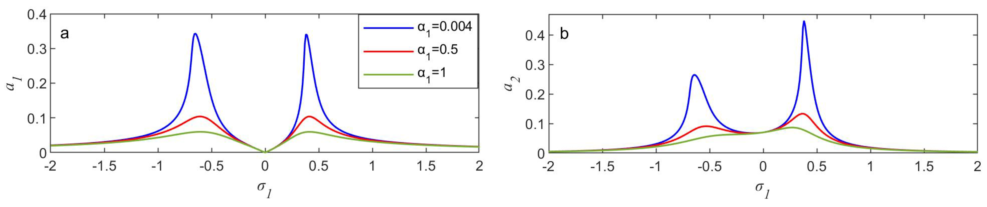
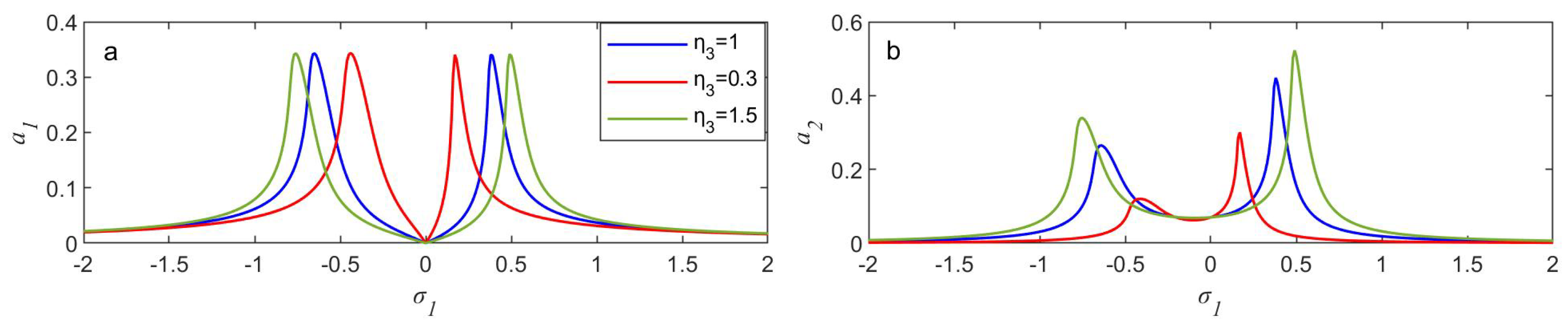
• Raising the NINDF parameter ${\eta }_1$ causes the curves to tilt to the right, which can enhance the NINDF controller’s effectiveness, especially when it comes to reducing high-amplitude vibrations in the nonlinear system.
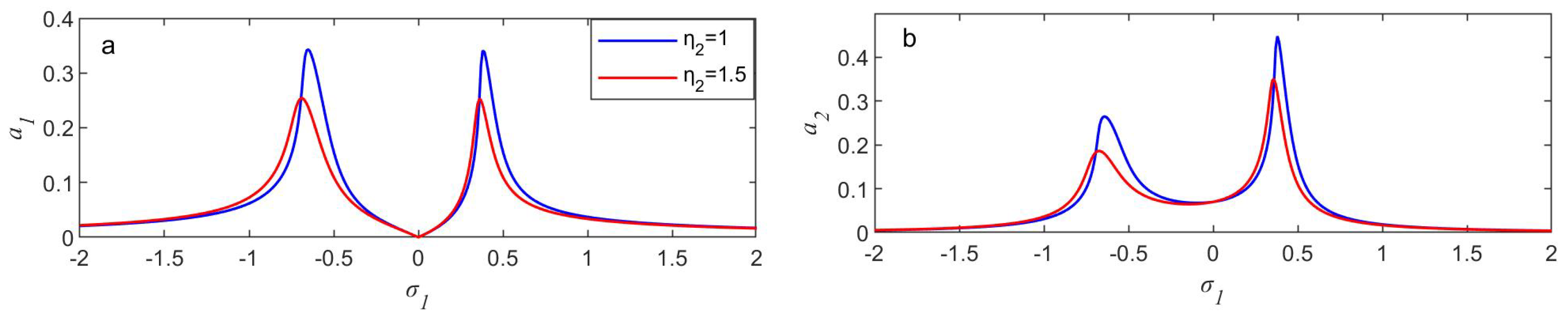
• The measured system’s amplitude diminishes exceedingly gradually for the NINDF parameter.
• The vibrating cantilever beam’s smallest amplitudes occur when ${\sigma }_1={\sigma }_2$.
• When the gains of the control signals ${\eta }_i$ ($i=1,2,3,4$) are increased, the NINDF controller’s reduction in vibration frequency bandwidth expands.
• The approximate and numerical solutions are in satisfactory agreement.

References

- Fryba, L. Vibration of Solids and Structures Under Moving Loads; Academia: Prague, Czech Republic, 1972. [Google Scholar]
- Kevin, M.; Dowell, E. Nonlinear responses of inextensible cantilever and free–free beams undergoing large deflections. J. Appl. Mech. 2018, 85, 051008. [Google Scholar]
- Dwivedy, S.K.; Kar, R.C. Nonlinear dynamics of a cantilever beam carrying an attached mass with 1: 3: 9 internal resonances. Nonlinear Dyn. 2003, 31, 49–72. [Google Scholar] [CrossRef]
- Kar, R.C.; Dwivedy, S.K. Non-linear dynamics of a slender beam carrying a lumped mass with principal parametric and internal resonances. Int. J. Non-Linear Mech. 1999, 34, 515–529. [Google Scholar] [CrossRef]
- Hamdan, M.N.; Shabaneh, N.H. On the large amplitude free vibrations of a restrained uniform beam carrying an intermediate lumped mass. J. Sound Vib. 1997, 199, 711–736. [Google Scholar] [CrossRef]
- Hamdan, M.N.; Dado, M.H.F. Large amplitude free vibrations of a uniform cantilever beam carrying an intermediate lumped mass and rotary inertia. J. Sound Vib. 1997, 206, 151–168. [Google Scholar] [CrossRef]
- Al-Qaisia, A.A.; Hamdan, M.N. Bifurcations of approximate harmonic balance solutions and transition to chaos in an oscillator with inertial and elastic symmetric nonlinearities. J. Sound Vib. 2001, 244, 453–479. [Google Scholar] [CrossRef]
- Al-Qaisia, A.A.; Hamdan, M.N. Bifurcations and chaos of an immersed cantilever beam in a fluid and carrying an intermediate mass. J. Sound Vib. 2002, 253, 859–888. [Google Scholar] [CrossRef]
- Gen, G.; Xie, N. An approach dealing with inertia nonlinearity of a cantilever model subject to lateral basal Gaussian white noise excitation. Chaos Solitons Fractals 2020, 131, 109469. [Google Scholar]
- Qian, Y.H.; Lai, S.K.; Zhang, W.; Xiang, Y. Study on asymptotic analytical solutions using HAM for strongly nonlinear vibrations of a restrained cantilever beam with an intermediate lumped mass. Numer. Algorithms 2011, 58, 293–314. [Google Scholar] [CrossRef]
- Yang, X.-J.; Gao, F.; Srivastava, H.M. A new computational approach for solving nonlinear local fractional PDEs. J. Comput. Appl. Math. 2018, 339, 285–296. [Google Scholar] [CrossRef]
- Ahmad, E.-A. A modification to the conformable fractional calculus with some applications. Alex. Eng. J. 2020, 59, 2239–2249. [Google Scholar]
- El-Nabulsi, R.A. On a new fractional uncertainty relation and its implications in quantum mechanics and molecular physics. Proc. R Soc. A 2020, 476, 20190729. [Google Scholar] [CrossRef]
- Chen, S.-S. Application of the differential transformation method to the free vibrations of strongly non-linear oscillators. Nonlinear Anal. Real World Appl. 2009, 10, 881–888. [Google Scholar] [CrossRef]
- Moatimid, M.; Amer, T.S.; Ellabban, Y.Y. A novel methodology for a time-delayed controller to prevent nonlinear system oscillations. J. Low Freq. Noise Vib. Act. Control 2024, 43, 525–542. [Google Scholar] [CrossRef]
- Abadi. Nonlinear Dynamics of Self-Excitation in Autoparametric Systems; Faculteit Wiskunde en Informatica, Universiteit Utrecht: Surabaya, Indonesia, 2003. [Google Scholar]
- El-Badawy, A.A.; El-Deen, T.N.N. Quadratic nonlinear control of a self-excited oscillator. J. Vib. Control 2007, 13, 403–414. [Google Scholar] [CrossRef]
- Li, J.; Li, X.; Hua, H. Active nonlinear saturation-based control for suppressing the free vibration of a self-excited plant. Commun. Nonlinear Sci. Numer. Simul. 2010, 15, 1071–1079. [Google Scholar]
- Warminski, J.; Cartmell, M.P.; Mitura, A.; Bochenski, M. Active Vibration Control of a Nonlinear Beam with Self-and External Excitations. Shock Vib. 2013, 20, 1033–1047. [Google Scholar] [CrossRef]
- Akash, S.; Mondal, J.; Chatterjee, S. Controlling self-excited vibration using positive position feedback with time-delay. J. Braz. Soc. Mech. Sci. Eng. 2020, 42, 1–10. [Google Scholar]
- Saeed, N.A.; Awrejcewicz, J.; Alkashif, M.A.; Mohamed, M.S. 2D and 3D visualization for the static bifurcations and nonlinear oscillations of a self-excited system with time-delayed controller. Symmetry 2022, 14, 621. [Google Scholar] [CrossRef]
- Joy, M.; Chatterjee, S. Controlling self-excited vibration of a nonlinear beam by nonlinear resonant velocity feedback with time-delay. Int. J. Non-Linear Mech. 2021, 131, 103684. [Google Scholar]
- Akash, S.; Mondal, J.; Chatterjee, S. Controlling self-excited vibration using acceleration feedback with time-delay. Int. J. Dyn. Control 2019, 7, 1521–1531. [Google Scholar]
- Amer, Y.A.; El-Sayed, A.T.; Abd El-Salam, M.N. Non-linear saturation controller to reduce the vibrations of vertical conveyor subjected to external excitation. Asian Res. J. Math. 2018, 11, 1–26. [Google Scholar] [CrossRef]
- Amer, Y.A.; Abd EL-Salam, M.N. Negative Derivative Feedback Controller for Repressing Vibrations of the Hybrid Rayleigh-Van der Pol-Duffing Oscillator. Nonlinear Phenom. Complex Syst. 2022, 25, 217–228. [Google Scholar] [CrossRef]
- Nayfeh, A.H. Perturbation Methods; John Wiley and Sons: New York, NY, USA, 1973. [Google Scholar]
- Bauomy, H.S.; El-Sayed, A.T. Mixed controller (IRC+ NSC) involved in the harmonic vibration response cantilever beam model. Meas. Control 2020, 53, 1954–1967. [Google Scholar] [CrossRef]
- Amer, Y.A.; EL-Sayed, A.T.; Abd EL-Salam, M.N. A suitable active control for suppression the vibrations of a cantilever beam. Sound. Vib. 2022, 56, 89–104. [Google Scholar] [CrossRef]