Transverse Wave Propagation in Functionally Graded Structures Using Finite Elements with Perfectly Matched Layers and Infinite Element Coupling

Abstract

This study investigates the propagation of shear horizontal transverse waves in a functionally graded piezoelectric half-space (FGPHS), where the material properties vary linearly and quadratically. The analysis focuses on deriving and understanding the dispersion characteristics of such waves in in-homogeneous media. The WKB approximation method is employed to obtain the dispersion relation analytically, considering the smooth variation of material properties. To validate and study the wave behavior numerically, two advanced techniques were utilized: the Semi-Analytical Finite Element with Perfectly Matched Layer (SAFE-PML) and the Semi-Analytical Infinite Element (SAIFE) method incorporating a (1/r) decay model to simulate infinite media. The numerical implementation uses the Rayleigh–Ritz method to discretize the wave equation, and Gauss 3-point quadrature is applied for efficient numerical integration. The dispersion curves are plotted to illustrate the wave behavior in the graded piezoelectric medium. The results from SAFE-PML and SAIFE are in excellent agreement, indicating that these techniques effectively model the shear horizontal transverse wave propagation in such structures. This study also demonstrates that combining finite and infinite element approaches provides accurate and reliable simulation of wave phenomena in functionally graded piezoelectric materials, which has applications in sensors, actuators, and non-destructive testing.

1. Introduction

Piezoelectric materials, distinguished by their unique ability to interconvert mechanical and electrical energy, have garnered considerable attention from researchers and engineers owing to their exceptional properties. The term “piezoelectric” finds its origins in the Greek word “piezein”, which translates to “to squeeze” or “to press.” When a piezoelectric material is squeezed or pressed, it generates a measurable electrical voltage across its surface. The versatility and efficiency of piezoelectric materials have led to their integration into a vast array of devices and technologies. From the simple piezoelectric lighters used in everyday life to sophisticated medical imaging systems and precision actuators employed in industrial processes. These materials play a crucial role in shaping the way we interact with and harness energy from our environment.

The concept of functionally graded materials (FGMs) originated from the aspiration to customize material properties to specific needs. Functionally graded piezoelectric materials (FGPMs) are designed to possess varying piezoelectric coefficients, elastic constants, or dielectric properties along specific directions. This gradient allows the material to adapt and respond optimally to varying mechanical or electrical stimuli. Extensive research on wave propagation in functionally graded materials and functionally graded piezoelectric materials has been carried out by several prominent scholars, including Liu et al. [1], Han et al. [2,3], Liu and Tani [4,5], and Han and Liu [6,7].

Li et al. [8] analyzed the behavior of Love waves in multilayered structures composed of functionally graded piezoelectric materials. Chaudhary et al. [9] developed a theoretical model describing Rayleigh wave propagation in a piezoelectric layer bonded to an orthotropic substrate. Furthermore, Qian et al. [10] investigated the propagation of transverse surface waves in a polarized piezoelectric half-space overlaid with a functionally graded material layer. Using the framework of linear piezoelectricity, Chaki et al. [11] explored the dispersion characteristics of anti-plane surface waves, particularly Love waves, within a system composed of a homogeneous, fully coupled magneto-electro-elastic layer over a half-space.

Qian et al. [12] studied how in-homogeneous initial stresses influence the dispersion relations and phase velocities of Love waves. Jin et al. [13] focused on how both homogeneous and in-homogeneous initial stresses affect surface wave transmission in piezoelectric materials. Han et al. [14] employed numerical methods to investigate transient wave propagation in functionally graded material plates subjected to impact loads. Singh and Prasad [15] examined the propagation of shear horizontal (SH) surface waves over a magneto-electro-elastic (MEE) substrate patterned with periodic gold strips separated by a vacuum. Akshaya et al. [16] analyzed SH wave transmission between two imperfectly bonded, functionally graded half-spaces. Hemalatha and Kumar [17] investigated SH wave propagation in a rotating functionally graded magneto-electro-elastic material (FGMEE) with an imperfect interface. Recent investigations have focused on SH wave propagation in functionally graded and magneto-electro-elastic structures, considering the effects of interface imperfections and corrugation [18,19,20].

The Wentzel–Kramers–Brillouin (WKB) approximation offers an effective method for approximating solutions to linear differential equations with spatially varying coefficients. In this approach, the wave function is expressed in an exponential form and then expanded semiclassically, based on the assumption that either the amplitude or the phase changes slowly. The WKB method also establishes a connection between classical and quantum mechanics, as discussed by Froman and Froman [21]. Cerveny and Ravindra [22] further developed a comprehensive framework for elastic wave propagation in in-homogeneous layered media based on direct asymptotic expansion. Additionally, Kumar et al. [23] applied the WKB technique to study shear surface wave behavior in piezoelectric structures featuring imperfectly bonded piezoelectric layers. Morsbol et al. [24] also utilized the WKB approximation to investigate the properties of elastic waveguides, specifically analyzing an unbounded pipe with a circular cross-section whose radius varies gradually along its length.

Liu and Wang [25] applied the WKB method to investigate the propagation of Love waves in a functionally graded multilayer piezoelectric structure. Similarly, Du et al. [26] analyzed the dispersion characteristics of Love waves in various FGPM multilayer systems using the WKB approach. Han et al. [27] addressed the issue of Love wave propagation across imperfectly bonded interfaces and derived approximate solutions through the WKB method. Holubets et al. [28] utilized the WKB technique to study wave propagation in a non-homogeneous porous plate with a gradually varying refractive index. Furthermore, Qian et al. [29] explored the behavior of Love waves under initial stress conditions in a layered, functionally graded, non-piezoelectric half-space using the WKB method.

The finite element method (FEM) is a numerical approach employed for tackling intricate engineering and mathematical challenges by partitioning them into smaller, more manageable subdomains known as finite elements. It finds extensive application across diverse domains such as structural analysis, heat transfer, fluid dynamics, and electromagnetics. Roy et al. [30] worked on improving the eight-node layered shell finite element model to better capture the piezothermoelastic response of smart fiber-reinforced polymer (FRP) composite shells embedded with bonded piezoelectric sensors and actuators. In a related study, De et al. [31] applied the semi-analytical finite element method (SAFEM) to determine the effective material properties of piezoelectric fiber-reinforced composites (PFRC). To simulate wave absorption effectively, the perfectly matched layer (PML) technique was introduced by incorporating complex coordinate stretching and applying analytical continuation of the governing equations. Several researchers [32,33,34,35,36] have explored different forms of stretching functions to implement the PML approach successfully. Numerous research efforts have explored the application of infinite elements to simulate unbounded media, achieving significant success in solving wave propagation problems [37,38,39,40,41,42,43,44].

Functionally graded piezoelectric materials are emerging as promising candidates for a wide range of applications, including energy harvesting, sensing, actuation, and biomedical engineering. Their versatility continues to drive substantial research interest in this field. This study offers a novel exploration that integrates both analytical and numerical methods to investigate the dispersion behavior of transverse waves in a half-space structure composed of FGPMs, considering both linear and quadratic gradation profiles. Such a thorough and combined analysis has not been previously reported. To effectively model the half-space and address absorbing boundary conditions, a semi-analytical finite element–perfectly matched layer (SAFE-PML) framework is developed, employing complex coordinate transformations and Dirichlet-type boundary conditions at the lower boundary of the PML.

In addition, a semi-analytical infinite element (SAIFE) method with a $(1/r)$ decay behavior is utilized. Assembly-level formulations are established for both the SAFE-PML and SAIFE techniques, accommodating different gradation parameters to accurately capture the dispersion properties of shear horizontal wave propagation. The dispersion relations are further obtained using an analytical Wentzel–Kramers–Brillouin approximation. Extensive numerical studies, based on results from the analytical WKB approach, SAFE-PML, and SAIFE $(1/r)$ methods, are carried out to systematically examine the effects of various influencing factors on wave propagation characteristics.

In this study, we aim to bridge this gap by investigating the dispersion behavior of SH waves in a functionally graded half-space, where material properties change linearly and quadratically along the depth. To achieve this, we adopt a combined analytical and numerical approach. On the analytical side, we employ the Wentzel–Kramers–Brillouin (WKB) approximation to derive dispersion relations considering a gradual material variation. Two semi-analytical methods were introduced. These are the semi-analytical finite element method with a perfectly matched layer (SAFE-PML). This technique handles absorbing boundaries through complex coordinate transformation. The second approach is the semi-analytical infinite element (SAIFE) method, which uses a $1/r$ decay model to simulate infinite media.

The main objectives of this work are to develop accurate models for SH wave propagation in FGPMs, to evaluate how different gradation profiles influence dispersion, and finally to provide a robust framework that integrates both analytical insights and numerical simulations. By combining these approaches, we hope to offer a deeper understanding of wave behavior in in-homogeneous piezoelectric media and contribute a novel methodology that can be extended to future studies in smart and functionally graded materials.

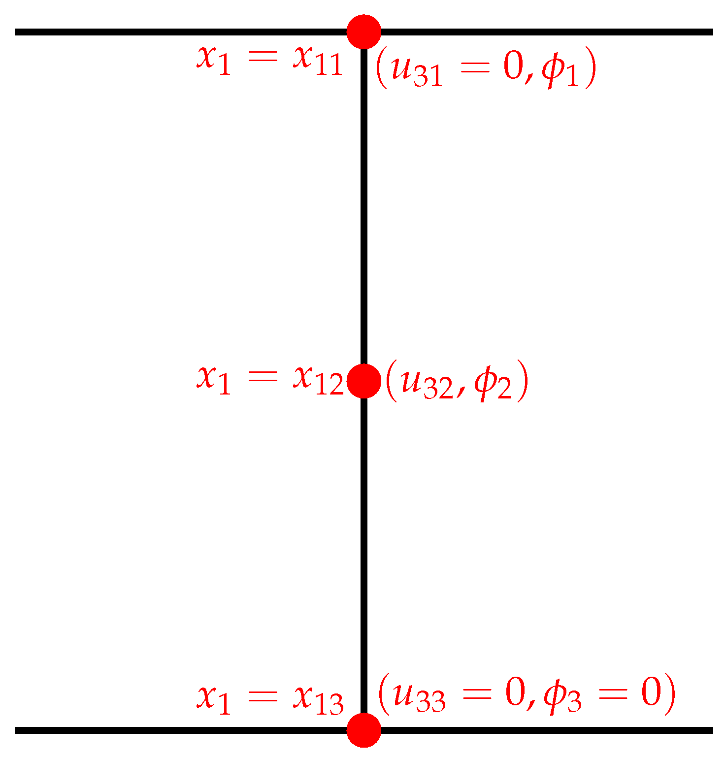
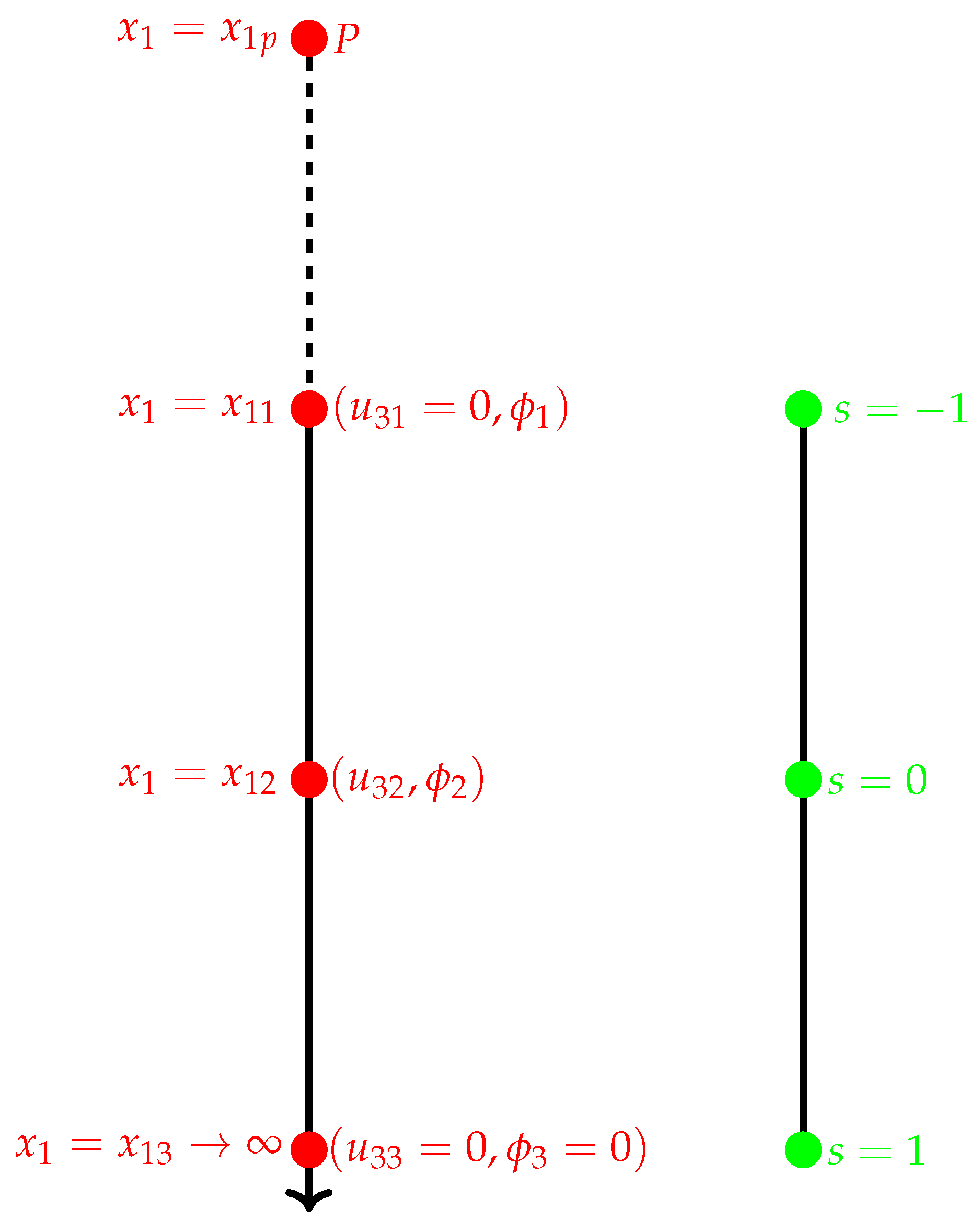
2. Problem Formulation

In this section, we examine the behavior of a horizontally polarized shear (SH) wave as it propagates through a functionally graded piezoelectric half-space (FGPHS). The field equations of the FGPHS can be expressed as follows:

$$\begin{array}{c}\hfill T_{ij,j}=\rho {\ddot{u}}_i,D_{i,i}=0\end{array}$$

(1)

in this context, $i,j$ = $1,2,3$, $\rho$ denotes the mass density, while $D_i$ and $u_i$ represent the electric and mechanical displacements along the i-th direction, respectively. The stress tensor is symbolized by $T_{ij}$. The dot over a variable indicates differentiation with respect to time while the comma denotes spatial differentiation, and double indices commas imply summation according to the Einstein summation convention. The SH wave propagation is considered along the positive $x_2$ direction and does not vary along the $x_3$ direction. The scalar potential function and the mechanical displacement components are expressed as follows:

$$\begin{array}{c}\hfill u_1=0,u_2=0,u_3=u_3\left(x_1,x_2,t\right),\varphi =\varphi \left(x_1,x_2,t\right)\end{array}$$

(2)

In the half-space region defined by $-\infty <x_1<0$, the mechanical displacement is denoted by ($u_3$), while the electric potential is described by ($\varphi$). Therefore, the governing equation for SH wave propagation in a half-space [16] can be derived as

$$\begin{array}{c}\hfill T_{31,1}+T_{23,2}=\rho {\ddot{u}}_3\end{array}$$

(3)

and

$$\begin{array}{c}\hfill D_{1,1}+D_{2,2}=0\end{array}$$

(4)

In this context, $T_{31}$ and $T_{32}$ denote the stress components, while $D_1$ and $D_2$ correspond to the electric displacement components within the FGPHS, respectively. Moreover, $u_3$ represents the mechanical displacement along the $x_3$ axis, and $\rho$ refers to the density of the FGPHS. The connections among stress, electric displacement, and their corresponding mechanical and electrical displacements are described as follows

$$\begin{array}{cc}\hfill T_{31}& =C_{44}\left(x_1\right)u_{3,1}+e_{15}\left(x_1\right){\varphi }_{,1}\hfill \\ \hfill T_{23}& =C_{44}\left(x_1\right)u_{3,2}+e_{15}\left(x_1\right){\varphi }_{,2}\hfill \end{array}$$

(5)

$$\begin{array}{cc}\hfill D_1& =e_{15}\left(x_1\right)u_{3,1}-{\kappa }_{11}\left(x_1\right){\varphi }_{,1}\hfill \\ \hfill D_2& =e_{15}\left(x_1\right)u_{3,2}-{\kappa }_{11}\left(x_1\right){\varphi }_{,2}\hfill \end{array}$$

(6)

$$\begin{array}{c}\hfill \rho =\rho \left(x_1\right)\end{array}$$

(7)

The field equations that govern the behavior of the FGPHS are given by Equations (3)–(7)

$$\begin{array}{c}\hfill C_{44}\left(u_{3,11}+u_{3,22}\right)+e_{15}\left({\varphi }_{,11}+{\varphi }_{,22}\right)+{C_{44}}^{\prime }{u}_{3,1}+{e_{15}}^{\prime }{\varphi }_{,1}=\rho {\ddot{u}}_3\end{array}$$

(8)

$$\begin{array}{c}\hfill e_{15}\left(u_{3,11}+u_{3,22}\right)-{\kappa }_{11}\left({\varphi }_{,11}+{\varphi }_{,22}\right)+{e_{15}}^{\prime }{u}_{3,1}-{{\kappa }_{11}}^{\prime }{\varphi }_{,1}=0\end{array}$$

(9)

where Equations (8) and (9) are the result of replacing expressions of Equations (5) and (6) in Equations (3) and (4), respectively. The prime represents differentiation with respect to $x_1$. The material parameters of the FGPHS are considered to be any function such that

$$\begin{array}{c}\hfill C_{44}\left(x_1\right)=C_{44}f\left(x_1\right),e_{15}\left(x_1\right)=e_{15}f\left(x_1\right),{\kappa }_{11}\left(x_1\right)={\kappa }_{11}f\left(x_1\right),\rho \left(x_1\right)=\rho f\left(x_1\right)\end{array}$$

(10)

Thus, the mechanical, electric, and magnetic conditions at the interface of FGPHS at $x_1=0$ are

$$\begin{array}{c}\hfill T_{31}=0,u_3=0,\varphi =0,D_1=0\end{array}$$

(11)

3. Semi-Analytic Finite Element (SAFE) and Perfectly Matched Layer (PML) Techniques

The finite element analysis starts by discretizing the half-space into three-noded elements. Within each element, the mechanical displacement $u_3$ and the electric potential $\varphi$ are approximated as follows

$$\begin{array}{c}\hfill u_3=\sum _{j=1}^3{N}_j{\left\{u_j\right\}}^e,\varphi =\sum _{j=1}^3{N}_j{\left\{{\varphi }_j\right\}}^e\end{array}$$

(12)

Then, let ${u_j}^e$ and ${{\varphi }_j}^e$ represent the nodal values of $u_3$ and $\varphi$ at the j-th node of the e-th finite element, respectively. Therefore, within each element, we introduce quadratic shape functions $N_j$, which are defined based on the local coordinate $x_2^{\prime }$ and the element length $h_e$. These parameters are expressed as

$$\begin{array}{c}\hfill N_1=(1-{\displaystyle \frac{x_1^{\prime }}{h_e}})(1-{\displaystyle \frac{2x_1^{\prime }}{h_e}}),N_2={\displaystyle \frac{4x_1^{\prime }}{h_e}}(1-{\displaystyle \frac{x_1^{\prime }}{h_e}}),N_3={\displaystyle \frac{x_1^{\prime }}{h_e}}({\displaystyle \frac{2x_1^{\prime }}{h_e}}-1)\end{array}$$

(13)

3.1. Weak Form of the Problem

To solve the above equation, we assume a solution that exhibits harmonic time dependence which is expressed as

$$\begin{array}{c}\hfill \left\{u_3,\varphi \right\}(x_1,x_2,t)=\left\{u_3,\varphi \right\}(x_1,x_2)e^{i\omega t}\end{array}$$

(14)

Then, setting the weighted-residuals of Equations (3) and (4) to zero as

$$\begin{array}{c}\hfill {\int }_{{\Omega }_e}{w}_t(T_{31,1}+T_{23,2}-\rho u_3{\omega }^2)d{\Omega }_e=0\end{array}$$

(15)

and

$$\begin{array}{c}\hfill {\int }_{{\Omega }_e}{w}_t(D_{1,1}+D_{2,2})d{\Omega }_e=0\end{array}$$

(16)

Here, $\omega =kc$ denotes the angular frequency, $w_t$ is the weight function, and ${\Omega }_e=d{x}_1,d{x}_2$ represents the domain of the e-th element. Then, applying integration by parts to Equations (15) and (16), and utilizing the component-wise representation of the Gradient theorem, we obtain the weak form of these equations as follows

$$\begin{array}{c}\hfill {\int }_{{\Omega }_e}(T_{31}{w}_{t,1}+T_{23}{w}_{t,2}-\rho u_3{\omega }^2{w}_t)d{\Omega }_e={\oint }_{{\gamma }_e}\left[\left(w_t{T}_{31}\right)n_1+\left(w_t{T}_{23}\right)n_2\right]dS\end{array}$$

(17)

and

$$\begin{array}{c}\hfill {\int }_{{\Omega }_e}(D_1{w}_{t,1}+D_2{w}_{t,2})d{\Omega }_e={\oint }_{{\gamma }_e}\left[\left(w_t{D}_1\right)n_1+\left(w_t{D}_2\right)n_2\right]dS\end{array}$$

(18)

where ${\gamma }_e$ signifies the boundary surface of the e-th element, and $(n_1,n_2)$ are the direction cosines associated with this boundary surface. Leveraging the variational framework of the Rayleigh–Ritz method, we set $w_t=N_i$. Then, using Equations (4)–(11), (17), and (18) for the full-model equation of FGPHS results in

$$\begin{array}{c}\hfill \sum _{j=1}^3{\left\{K_{ij}^{\left(1\right)}\right\}}^e{\left\{u_j\right\}}^e+\sum _{j=1}^3{\left\{K_{ij}^{\left(2\right)}\right\}}^e{\left\{{\varphi }_j\right\}}^e-{\omega }^2\sum _{j=1}^3{\left\{M_{ij}^{\left(1\right)}\right\}}^e{\left\{u_j\right\}}^e={\left\{Q_i^{\left(1\right)}\right\}}^e\end{array}$$

(19)

$$\begin{array}{c}\hfill \sum _{j=1}^3{\left\{K_{ij}^{\left(2\right)}\right\}}^e{\left\{u_j\right\}}^e+\sum _{j=1}^3{\left\{K_{ij}^{\left(3\right)}\right\}}^e{\left\{{\varphi }_j\right\}}^e={\left\{Q_i^{\left(2\right)}\right\}}^e\end{array}$$

(20)

where

$$\begin{array}{c}\hfill {\left\{K_{ij}^{\left(1\right)}\right\}}^e={\int }_{{\Omega }_e}{C}_{44}f\left(x_1\right)(N_{i,1}{N}_{j,1}+N_{i,2}{N}_{j,2})d{\Omega }_e\end{array}$$

(21)

$$\begin{array}{c}\hfill {\left\{K_{ij}^{\left(2\right)}\right\}}^e={\int }_{{\Omega }_e}{e}_{15}f\left(x_1\right)(N_{i,1}{N}_{j,1}+N_{i,2}{N}_{j,2})d{\Omega }_e\end{array}$$

(22)

$$\begin{array}{c}\hfill {\left\{K_{ij}^{\left(3\right)}\right\}}^e=-{\int }_{{\Omega }_e}{\kappa }_{11}f\left(x_1\right)(N_{i,1}{N}_{j,1}+N_{i,2}{N}_{j,2})d{\Omega }_e\end{array}$$

(23)

$$\begin{array}{c}\hfill {\left\{M_{ij}^{\left(1\right)}\right\}}^e={\int }_{{\Omega }_e}f\left(x_1\right)\left[\rho N_i{N}_j\right]d{\Omega }_e\end{array}$$

(24)

$$\begin{array}{c}\hfill {\left\{Q_i^{\left(1\right)}\right\}}^e={\oint }_{{\gamma }_e}\left[N_i(T_{31}{n}_1+T_{23}{n}_2)\right]dS\end{array}$$

(25)

$$\begin{array}{c}\hfill {\left\{Q_i^{\left(2\right)}\right\}}^e={\oint }_{{\gamma }_e}\left[N_i(D_1{n}_1+D_2{n}_2)\right]dS\end{array}$$

(26)

3.2. SAFE Technique

Here, we hypothesize a solution form that varies spatially as follows:

$$\begin{array}{c}\hfill \left\{u_3,\varphi \right\}(x_1,x_2)=\left\{u_3,\varphi \right\}\left(x_1\right)e^{ik{x}_2}\end{array}$$

(27)

Therefore, using Equations (21)–(27) for the FGPHS yields

$$\begin{array}{c}\hfill {\left\{K_{ij}^{\left(1\right)}\right\}}^e={\int }_{x_{1e}}{C}_{44}f\left(x_1\right)(N_{i,1}{N}_{j,1}-k^2{N}_i{N}_j)d{x}_1\end{array}$$

(28)

$$\begin{array}{c}\hfill {\left\{K_{ij}^{\left(2\right)}\right\}}^e={\int }_{x_{1e}}{e}_{15}f\left(x_1\right)(N_{i,1}{N}_{j,1}-k^2{N}_i{N}_j)d{x}_1\end{array}$$

(29)

$$\begin{array}{c}\hfill {\left\{K_{ij}^{\left(3\right)}\right\}}^e=-{\int }_{x_{1e}}{\kappa }_{11}f\left(x_1\right)(N_{i,1}{N}_{j,1}-k^2{N}_i{N}_j)d{x}_1\end{array}$$

(30)

$$\begin{array}{c}\hfill {\left\{M_{ij}^{\left(1\right)}\right\}}^e={\int }_{x_{1e}}\left[\rho f\left(x_1\right)N_i{N}_j\right]d{x}_1\end{array}$$

(31)

$$\begin{array}{c}\hfill {\left\{Q_i^{\left(1\right)}\right\}}^e=\left(N_i{T}_{31}{n}_1\right){|}_{x_{1i}}\end{array}$$

(32)

$$\begin{array}{c}\hfill {\left\{Q_i^{\left(2\right)}\right\}}^e=\left(N_i{D}_1{n}_1\right){|}_{x_{1i}}\end{array}$$

(33)

3.3. PML Technique

To implement the PML method along the $x_1$ axis, Equations (17) and (18) are reformulated by extending the equilibrium equations into a complex plane. This involves replacing the real coordinate $x_1$ with a complex variable denoted by ${\tilde{x}}_1$. The precise relationship between $x_1$ and ${\tilde{x}}_1$ is described by

$$\begin{array}{c}\hfill {\tilde{x}}_1={\int }_0^{x_1}\lambda \left(s\right)ds\end{array}$$

(34)

Here, s denotes a continuous, complex-valued stretching function of $x_1$ that does not vanish anywhere. Under the coordinate transformation ${\tilde{x}}_1\to x_1$, the differential elements are related by $d{\tilde{x}}_1=\lambda d{x}_1$. Where $x_1>0$, and the area is designated as a PML of a length of l, with $x_2$ ranging over an interval of $[0,l]$. At the terminating boundary $x_1=l$, the Dirichlet boundary conditions are applied once setting $u_3=0$ and $\varphi =0$.

3.4. Coordinate Transformation

To simplify the numerical integration, we define s as a natural coordinate system. It spans in the range of ($-1\le s\le 1$). Here, the system is designed to encompass the full length l of a 3-node element, and the mapping from the local coordinate system $x_2^{\prime }$ to the natural coordinate system s is given by

$$\begin{array}{c}\hfill x_1^{\prime }\left(s\right)=\sum _{j=1}^3{\alpha }_j\left(s\right){x_{1j}}^{\prime }\end{array}$$

(35)

where ${\alpha }_j$ represents the 3-point Lagrangian interpolation functions defined as

$$\begin{array}{c}\hfill {\alpha }_1\left(s\right)={\displaystyle \frac{1}{2}}s(s-1),{\alpha }_2\left(s\right)=(1-s^2),{\alpha }_3\left(s\right)={\displaystyle \frac{1}{2}}s(s+1)\end{array}$$

(36)

Then, by defining $x_{11}^{\prime }$, $x_{12}^{\prime }$, and $x_{13}^{\prime }$ as the initial point, midpoint, and final point of the element, respectively, the Jacobian transformation that maps $x_1^{\prime }$ to s in Equation (35) is written as

$$\begin{array}{c}\hfill J_1={\displaystyle \frac{d{x}_1^{\prime }}{ds}}={\displaystyle \frac{x_{13}^{\prime }-x_{11}^{\prime }}{2}}\end{array}$$

(37)

After that, applying the transformation form, Equations (13)–(35) yield

$$\begin{array}{c}\hfill N_1={\displaystyle \frac{1}{2}}s(s-1),N_2=(1-s^2),N_3={\displaystyle \frac{1}{2}}s(s+1)\end{array}$$

(38)

Thus, Equation (12) is rewritten as

$$\begin{array}{c}\hfill u_3=\sum _{j=1}^3{\alpha }_j{\left\{u_j\right\}}^e,\varphi =\sum _{j=1}^3{\alpha }_j{\left\{{\varphi }_j\right\}}^e\end{array}$$

(39)

Taking into account the relations between Equations (35)–(39), the coefficients defined in Equations (28)–(33) are transformed into the following expressions

$$\begin{array}{c}\hfill {\left\{K_{ij}^{\left(1\right)}\right\}}^e={\int }_{-1}^1\left[C_{44}f\left[{\displaystyle \frac{(1+s)d}{2}}\right]\left({\displaystyle \frac{1}{{\left(\lambda J_1\right)}^2}}{\alpha }_{i,s}{\alpha }_{j,s}-k^2{\alpha }_i{\alpha }_j\right)\right]\lambda \left|J_1\right|ds\end{array}$$

(40)

$$\begin{array}{c}\hfill {\left\{K_{ij}^{\left(2\right)}\right\}}^e={\int }_{-1}^1\left[e_{15}f\left[{\displaystyle \frac{(1+s)d}{2}}\right]\left({\displaystyle \frac{1}{{\left(\lambda J_1\right)}^2}}{\alpha }_{i,s}{\alpha }_{j,s}-k^2{\alpha }_i{\alpha }_j\right)\right]\lambda \left|J_1\right|ds\end{array}$$

(41)

$$\begin{array}{c}\hfill {\left\{K_{ij}^{\left(3\right)}\right\}}^e=-{\int }_{-1}^1\left[{\kappa }_{11}f\left[{\displaystyle \frac{(1+s)d}{2}}\right]\left({\displaystyle \frac{1}{{\left(\lambda J_1\right)}^2}}{\alpha }_{i,s}{\alpha }_{j,s}-k^2{\alpha }_i{\alpha }_j\right)\right]\lambda \left|J_1\right|ds\end{array}$$

(42)

$$\begin{array}{c}\hfill {\left\{M_{ij}^{\left(1\right)}\right\}}^e={\int }_{-1}^1\left[\rho \left[{\displaystyle \frac{(1+s)d}{2}}\right]{\alpha }_i{\alpha }_j\right]\lambda \left|J_1\right|ds\end{array}$$

(43)

3.5. Assembly Process

Equations (19) and (20) represent the governing equations for the element e at a known level where the global degrees of freedom are illustrated in Figure 1. Thus, the element equations are assembled by incorporating the boundary conditions result in a set of coupled equations expressed as

$$\begin{array}{c}\hfill \left[K_{ij}\left(\omega \right)-{\omega }^2{M}_{ij}\left(\omega \right)\right]U_j=Q_j\end{array}$$

(44)

The coefficient $K_{ij}$ corresponds to the entries of the global stiffness $6\times 6$ matrix $\left[K\right]$, while $M_{ij}$ represents the elements of the global mass matrix with a similar size as the stiffness matrix. In addition, $U_j$ denotes the components of the vector U, and $Q_i$ represents the components of the vector Q, respectively. The following are the precise definitions of the terms:

$$\begin{array}{c}\hfill \left[\begin{array}{c}K\end{array}\right]=\left[\begin{array}{cccccc}{K}_{11}^{\left(1\right)}& K_{12}^{\left(1\right)}& K_{13}^{\left(1\right)}& K_{11}^{\left(2\right)}& K_{12}^{\left(2\right)}& K_{13}^{\left(2\right)}\\ K_{21}^{\left(1\right)}& K_{22}^{\left(1\right)}& K_{23}^{\left(1\right)}& K_{12}^{\left(2\right)}& K_{22}^{\left(2\right)}& K_{23}^{\left(2\right)}\\ K_{31}^{\left(1\right)}& K_{32}^{\left(1\right)}& K_{33}^{\left(1\right)}& K_{31}^{\left(2\right)}& K_{32}^{\left(2\right)}& K_{33}^{\left(2\right)}\\ K_{11}^{\left(2\right)}& K_{12}^{\left(2\right)}& K_{13}^{\left(2\right)}& -K_{11}^{\left(3\right)}& -K_{12}^{\left(3\right)}& -K_{13}^{\left(3\right)}\\ K_{21}^{\left(2\right)}& K_{22}^{\left(2\right)}& K_{23}^{\left(2\right)}& -K_{12}^{\left(3\right)}& -K_{22}^{\left(3\right)}& -K_{23}^{\left(3\right)}\\ K_{31}^{\left(2\right)}& K_{32}^{\left(2\right)}& K_{33}^{\left(2\right)}& -K_{31}^{\left(3\right)}& -K_{32}^{\left(3\right)}& -K_{33}^{\left(3\right)}\end{array}\right]\end{array}$$

(45)

$$\begin{array}{c}\hfill \left[\begin{array}{c}M\end{array}\right]=\left[\begin{array}{cccccc}{M}_{11}^{\left(1\right)}& M_{12}^{\left(1\right)}& M_{13}^{\left(1\right)}& 0& 0& 0\\ M_{21}^{\left(1\right)}& M_{22}^{\left(1\right)}& M_{23}^{\left(1\right)}& 0& 0& 0\\ M_{31}^{\left(1\right)}& M_{32}^{\left(1\right)}& M_{33}^{\left(1\right)}& 0& 0& 0\\ 0& 0& 0& 0& 0& 0& \\ 0& 0& 0& 0& 0& 0& \\ 0& 0& 0& 0& 0& 0& \end{array}\right]\end{array}$$

(46)

$$\begin{array}{c}\hfill \left[\begin{array}{c}U\end{array}\right]={\left[\begin{array}{cccccc}{u}_1& u_2& u_3& {\varphi }_1& {\varphi }_2& {\varphi }_3\end{array}\right]}^{\top }\end{array}$$

(47)

$$\begin{array}{c}\hfill \left[\begin{array}{c}Q\end{array}\right]={\left[\begin{array}{cccccc}\left(T_{31}{n}_1\right){|}_{x_{11}}& 0& 0& \left(D_1{n}_1\right){|}_{x_{12}}& 0& 0\end{array}\right]}^{\top }\end{array}$$

(48)

It is worth noting that the complex stretching function defined as (${\gamma }_2$) of the FGPHS may either vary with the frequency or remain independent of it when ${\gamma }_2$ is defined as ${\gamma }_2=f+f_i$. This results in global matrices that do not vary with $\omega$.

As a result, the eigenvalue problem becomes linear in ${\omega }^2$. On the other hand, if ${\gamma }_2$ is expressed as ${\gamma }_2={\displaystyle \frac{f+f_i}{\omega }}$, demarcating a frequency dependence, the global matrices depend on $\omega$. This leads to a higher-order eigenvalue problem that is a non-linear in $\omega$.

After applying the free surface boundary conditions from Equation (10) and the Dirichlet boundary conditions for the closed surface, Equation (45) simplifies to a $(3\times 3)$ eigenvalue problem in terms of $\omega$. Solving this eigenvalue problem provides the dispersion equation, which describes the propagation behavior of SH waves in the given half-space structure.

3.6. SAIFE Method with $(1/r)$ Decay Behavior

Here, we introduce a new method for approximating FGPHS, providing a different solution compared to the PML approach. The weak formulation of the equilibrium equations remains consistent with Equations (15) and (16). However, while the element-level equations retain the structure given in Equations (19) and (20), the domain approximation differs from the transformation in Equation (35). In its most basic form, we model the entire FGPHS using an infinite element.

Consider the 1-D element model shown in Figure 2, extending from node 1 $(x_1=x_{11})$ to node 2 $(x_1=x_{12})$ and further to node 3 $(x_1=x_{13})$, which extends infinitely. The pole position, $P(x_1=x_{1p})$, is chosen arbitrarily [37]. Thus,

$$\begin{array}{c}\hfill x_{14}=2x_{13}-x_{1p}\mathrm{with}{x}_{1p}\le x_{13}\end{array}$$

(49)

Also, it is assumed that $x_{1p}=x_{13}-l_1$, and thus $x_{14}-x_{13}=l_1$. Where $-1\le s\le 1$, the infinite element $x_{13}\le x_1\le \infty$ is mapped to the natural coordinate system using the following transformation:

$$\begin{array}{c}\hfill x_1\left(s\right)=\sum _{j=1}^3{\delta }_{j-2}\left(s\right)x_{1j}\end{array}$$

(50)

Here, the summation is limited to the finite nodes 1 and 2 corresponding to shape functions of ${\delta }_j$ that are defined as

$$\begin{array}{c}\hfill {\delta }_1\left(s\right)={\displaystyle \frac{-2s}{1-s}},{\delta }_2\left(s\right)={\displaystyle \frac{1+s}{1-s}}\end{array}$$

(51)

Taking into account Equation (50), we can solve Equation (49) to obtain

$$\begin{array}{c}\hfill s=1-{\displaystyle \frac{2l_1}{r}}\end{array}$$

(52)

where r represents the distance between the pole P and an arbitrary point located inside the element. The primary field variables, namely the transverse displacement $u_3$ and electric potential $\varphi$ in the FGPHS, are approximated using the standard Lagrangian interpolation functions as defined in Equations (36) and (39). Equation (39) is then obtained by systematically combining the relationships established in Equation (36) and the matrix form identify as (46), which results in

$$\begin{array}{cc}\hfill u_3& ={\displaystyle \frac{l_1}{r}}(-u_1+4u_2-u_3)+{\left({\displaystyle \frac{l_1}{r}}\right)}^2(2u_1-4u_2+2u_3)+u_3\hfill \\ \hfill \varphi & ={\displaystyle \frac{l_1}{r}}(-{\varphi }_1+4{\varphi }_2-{\varphi }_3)+{\left({\displaystyle \frac{l_1}{r}}\right)}^2(2{\varphi }_1-{\varphi }_2+2{\varphi }_3)+{\varphi }_3\hfill \end{array}$$

(53)

In analyzing anti-plane SH wave propagation, it is assumed that both the out-of-plane displacement and the electric potential vanish at infinite depth, i.e., $u_3\to 0$ and ${\varphi }_3\to 0$ as $r\to \infty$. Consequently, Equation (53) confirms that $u_3$ and $\varphi$ decay asymptotically following an inverse radial dependence, specifically of the form ($1/r$). Therefore, the subsequent equations represent the formulation at the element scale. So, the element-level equations are written as follows:

$$\begin{array}{c}\hfill {\left\{K_{ij}^{\left(1\right)}\right\}}^e={\int }_{-1}^1\left[C_{44}f\left[{\displaystyle \frac{(1+s)d}{2}}\right]\left({\displaystyle \frac{1}{{\left(J_2\right)}^2}}{\alpha }_{i,s}{\alpha }_{j,s}-k^2{\alpha }_i{\alpha }_j\right)\right]\left|J_2\right|ds\end{array}$$

(54)

$$\begin{array}{c}\hfill {\left\{K_{ij}^{\left(2\right)}\right\}}^e={\int }_{-1}^1\left[e_{15}f\left[{\displaystyle \frac{(1+s)d}{2}}\right]\left({\displaystyle \frac{1}{{\left(J_2\right)}^2}}{\alpha }_{i,s}{\alpha }_{j,s}-k^2{\alpha }_i{\alpha }_j\right)\right]\left|J_2\right|ds\end{array}$$

(55)

$$\begin{array}{c}\hfill {\left\{K_{ij}^{\left(3\right)}\right\}}^e=-{\int }_{-1}^1\left[{\kappa }_{11}f\left[{\displaystyle \frac{(1+s)d}{2}}\right]\left({\displaystyle \frac{1}{{\left(J_2\right)}^2}}{\alpha }_{i,s}{\alpha }_{j,s}-k^2{\alpha }_i{\alpha }_j\right)\right]\left|J_2\right|ds\end{array}$$

(56)

$$\begin{array}{c}\hfill {\left\{M_{ij}^{\left(1\right)}\right\}}^e={\int }_{-1}^1\left[\rho f\left[{\displaystyle \frac{(1+s)d}{2}}\right]{\alpha }_i{\alpha }_j\right]\left|J_2\right|ds\end{array}$$

(57)

4. Special Cases

In the present study, we consider the material properties of the FGPHS to vary either linearly or quadratically with respect to the spatial coordinate $x_1$. This gradedness assumption is motivated by both physical and analytical considerations. A linear variation represents a constant-rate transition of material properties, which serves as a first-order approximation of gradation and simplifies the mathematical formulation of the wave propagation problem. On the other hand, a quadratic variation accounts for non-uniform or accelerated changes in material parameters and offers a more accurate representation of the graded behavior observed in certain advanced functional materials. Incorporating such gradation enhances the effective properties of the piezoelectric medium and eliminates abrupt interfaces, thereby providing a more realistic modeling framework for analyzing the propagation characteristics.

4.1. Case 1

Here, we assume that the material gradedness parameter of the FGPHS varies linearly, that is, the FGPHS exhibits a linear functional distribution along the $x_1$-axis. This assumption is made because functional gradation enhances the properties of the piezoelectric half-space. Consequently, the material attributes of the FGPHS are classified as follows:

$$\begin{array}{cc}\hfill C_{44}\left(x_1\right)& =C_{44}[1+\alpha x_1]\hfill \\ \hfill e_{15}\left(x_1\right)& =e_{15}[1+\alpha x_1]\hfill \\ \hfill {\kappa }_{11}\left(x_1\right)& ={\kappa }_{11}[1+\alpha x_1]\hfill \\ \hfill \rho \left(x_1\right)& =\rho [1+\alpha x_1]\hfill \end{array}$$

(58)

Thus, Equations (40)–(43) become

$$\begin{array}{c}\hfill {\left\{K_{ij}^{\left(1\right)}\right\}}^e={\int }_{-1}^1\left[C_{44}\left(1+\alpha \left[{\displaystyle \frac{(1+s)d}{2}}\right]\right)\left({\displaystyle \frac{1}{{\left(\lambda J_1\right)}^2}}{\alpha }_{i,s}{\alpha }_{j,s}-k^2{\alpha }_i{\alpha }_j\right)\right]\lambda \left|J_1\right|ds\end{array}$$

(59)

$$\begin{array}{c}\hfill {\left\{K_{ij}^{\left(2\right)}\right\}}^e={\int }_{-1}^1\left[e_{15}\left(1+\alpha \left[{\displaystyle \frac{(1+s)d}{2}}\right]\right)\left({\displaystyle \frac{1}{{\left(\lambda J_1\right)}^2}}{\alpha }_{i,s}{\alpha }_{j,s}-k^2{\alpha }_i{\alpha }_j\right)\right]\lambda \left|J_1\right|ds\end{array}$$

(60)

$$\begin{array}{c}\hfill {\left\{K_{ij}^{\left(3\right)}\right\}}^e=-{\int }_{-1}^1\left[{\kappa }_{11}\left(1+\alpha \left[{\displaystyle \frac{(1+s)d}{2}}\right]\right)\left({\displaystyle \frac{1}{{\left(\lambda J_1\right)}^2}}{\alpha }_{i,s}{\alpha }_{j,s}-k^2{\alpha }_i{\alpha }_j\right)\right]\lambda \left|J_1\right|ds\end{array}$$

(61)

$$\begin{array}{c}\hfill {\left\{M_{ij}^{\left(1\right)}\right\}}^e={\int }_{-1}^1\left[\rho \left(1+\alpha \left[{\displaystyle \frac{(1+s)d}{2}}\right]\right){\alpha }_i{\alpha }_j\right]\lambda \left|J_1\right|ds\end{array}$$

(62)

Also, for the SAIFE technique Equations (54)–(57) become

$$\begin{array}{c}\hfill {\left\{K_{ij}^{\left(1\right)}\right\}}^e={\int }_{-1}^1\left[C_{44}\left(1+\alpha \left[{\displaystyle \frac{(1+s)d}{2}}\right]\right)\left({\displaystyle \frac{1}{{\left(J_2\right)}^2}}{\alpha }_{i,s}{\alpha }_{j,s}-k^2{\alpha }_i{\alpha }_j\right)\right]\left|J_2\right|ds\end{array}$$

(63)

$$\begin{array}{c}\hfill {\left\{K_{ij}^{\left(2\right)}\right\}}^e={\int }_{-1}^1\left[e_{15}\left(1+\alpha \left[{\displaystyle \frac{(1+s)d}{2}}\right]\right)\left({\displaystyle \frac{1}{{\left(J_2\right)}^2}}{\alpha }_{i,s}{\alpha }_{j,s}-k^2{\alpha }_i{\alpha }_j\right)\right]\left|J_2\right|ds\end{array}$$

(64)

$$\begin{array}{c}\hfill {\left\{K_{ij}^{\left(3\right)}\right\}}^e=-{\int }_{-1}^1\left[{\kappa }_{11}\left(1+\alpha \left[{\displaystyle \frac{(1+s)d}{2}}\right]\right)\left({\displaystyle \frac{1}{{\left(J_2\right)}^2}}{\alpha }_{i,s}{\alpha }_{j,s}-k^2{\alpha }_i{\alpha }_j\right)\right]\left|J_2\right|ds\end{array}$$

(65)

$$\begin{array}{c}\hfill {\left\{M_{ij}^{\left(1\right)}\right\}}^e={\int }_{-1}^1\left[\rho \left(1+\alpha \left[{\displaystyle \frac{(1+s)d}{2}}\right]\right){\alpha }_i{\alpha }_j\right]\left|J_2\right|ds\end{array}$$

(66)

4.2. Case 2

Here, we assume that the material gradedness parameter of the FGPHS varies quadratically; thus, the FGPHS exhibits a quadratic functional distribution along the $x_1$-axis. This assumption is made because functional gradation enhances the properties of the piezoelectric half-space. Consequently, the material attributes of the FGPHS are classified as follows:

$$\begin{array}{cc}\hfill C_{44}\left(x_1\right)& =C_{44}{[1+\alpha x_1]}^2\hfill \\ \hfill e_{15}\left(x_1\right)& =e_{15}{[1+\alpha x_1]}^2\hfill \\ \hfill {\kappa }_{11}\left(x_1\right)& ={\kappa }_{11}{[1+\alpha x_1]}^2\hfill \\ \hfill \rho \left(x_1\right)& =\rho {[1+\alpha x_1]}^2\hfill \end{array}$$

(67)

Then, Equations (40)–(43) become

$$\begin{array}{c}\hfill {\left\{K_{ij}^{\left(1\right)}\right\}}^e={\int }_{-1}^1\left[C_{44}{\left(1+\alpha \left[{\displaystyle \frac{(1+s)d}{2}}\right]\right)}^2\left({\displaystyle \frac{1}{{\left(\lambda J_1\right)}^2}}{\alpha }_{i,s}{\alpha }_{j,s}-k^2{\alpha }_i{\alpha }_j\right)\right]\lambda \left|J_1\right|ds\end{array}$$

(68)

$$\begin{array}{c}\hfill {\left\{K_{ij}^{\left(2\right)}\right\}}^e={\int }_{-1}^1\left[e_{15}{\left(1+\alpha \left[{\displaystyle \frac{(1+s)d}{2}}\right]\right)}^2\left({\displaystyle \frac{1}{{\left(\lambda J_1\right)}^2}}{\alpha }_{i,s}{\alpha }_{j,s}-k^2{\alpha }_i{\alpha }_j\right)\right]\lambda \left|J_1\right|ds\end{array}$$

(69)

$$\begin{array}{c}\hfill {\left\{K_{ij}^{\left(3\right)}\right\}}^e=-{\int }_{-1}^1\left[{\kappa }_{11}{\left(1+\alpha \left[{\displaystyle \frac{(1+s)d}{2}}\right]\right)}^2\left({\displaystyle \frac{1}{{\left(\lambda J_1\right)}^2}}{\alpha }_{i,s}{\alpha }_{j,s}-k^2{\alpha }_i{\alpha }_j\right)\right]\lambda \left|J_1\right|ds\end{array}$$

(70)

$$\begin{array}{c}\hfill {\left\{M_{ij}^{\left(1\right)}\right\}}^e={\int }_{-1}^1\left[\rho {\left(1+\alpha \left[{\displaystyle \frac{(1+s)d}{2}}\right]\right)}^2{\alpha }_i{\alpha }_j\right]\lambda \left|J_1\right|ds\end{array}$$

(71)

Also, for the SAIFE technique Equations (54)–(57) become

$$\begin{array}{c}\hfill {\left\{K_{ij}^{\left(1\right)}\right\}}^e={\int }_{-1}^1\left[C_{44}{\left(1+\alpha \left[{\displaystyle \frac{(1+s)d}{2}}\right]\right)}^2\left({\displaystyle \frac{1}{{\left(J_2\right)}^2}}{\alpha }_{i,s}{\alpha }_{j,s}-k^2{\alpha }_i{\alpha }_j\right)\right]\left|J_2\right|ds\end{array}$$

(72)

$$\begin{array}{c}\hfill {\left\{K_{ij}^{\left(2\right)}\right\}}^e={\int }_{-1}^1\left[e_{15}{\left(1+\alpha \left[{\displaystyle \frac{(1+s)d}{2}}\right]\right)}^2\left({\displaystyle \frac{1}{{\left(J_2\right)}^2}}{\alpha }_{i,s}{\alpha }_{j,s}-k^2{\alpha }_i{\alpha }_j\right)\right]\left|J_2\right|ds\end{array}$$

(73)

$$\begin{array}{c}\hfill {\left\{K_{ij}^{\left(3\right)}\right\}}^e=-{\int }_{-1}^1\left[{\kappa }_{11}{\left(1+\alpha \left[{\displaystyle \frac{(1+s)d}{2}}\right]\right)}^2\left({\displaystyle \frac{1}{{\left(J_2\right)}^2}}{\alpha }_{i,s}{\alpha }_{j,s}-k^2{\alpha }_i{\alpha }_j\right)\right]\left|J_2\right|ds\end{array}$$

(74)

$$\begin{array}{c}\hfill {\left\{M_{ij}^{\left(1\right)}\right\}}^e={\int }_{-1}^1\left[\rho {\left(1+\alpha \left[{\displaystyle \frac{(1+s)d}{2}}\right]\right)}^2{\alpha }_i{\alpha }_j\right]\left|J_2\right|ds\end{array}$$

(75)

5. Analytic Method

5.1. Solution for FGPHS for Linear Gradedness Parameter

To solve Equations (8) and (9), we propose the following form of the solution:

$$\begin{array}{c}\hfill \left\{u_3,\varphi \right\}(x_1,x_2,t)=\left\{U_3,\Phi \right\}\left(x_1\right)e^{ik(x_2-ct)}\end{array}$$

(76)

By inserting the solution form from Equation (76) into the governing Equations (8) and (9) for the functionally graded piezoelectric half-space (FGPHS) with a linear grading parameter, we use the WKB method to derive approximate expressions for the mechanical displacement and electric potential. The goal is to obtain depth-dependent decaying solutions that meet the required conditions of $u_3\to 0$ and $\varphi \to 0$ as $x_1\to -\infty$.

Then, the resulting approximate solutions are constructed following the methodology outlined in [16]. Furthermore, assuming $A^0$=$C_{44}$+$\left({\displaystyle \frac{{\left(e_{15}\right)}^2}{{\kappa }_{11}}}\right)$ and $a_1\left(x_1\right)=\left[1+\beta x_1\right]$, we can express $u_{31}$ and $\varphi \left(x_1,x_2,t\right)$ as

$$\begin{array}{c}\hfill u_{31}\left(x_1,x_2,t\right)={\displaystyle \frac{F_1{e}^{-i{s}_1\left(x_1\right)}}{\sqrt{1+\beta x_1}}}{e}^{ik\left(x_2-ct\right)}\end{array}$$

(77)

$$\begin{array}{c}\hfill \varphi \left(x_1,x_2,t\right)={\displaystyle \frac{F_2{e}^{-s_2\left(x_1\right)}}{\sqrt{1+\beta x_1}}}{e}^{ik\left(x_2-ct\right)}+{\displaystyle \frac{e_{15}}{{\kappa }_{11}}}{u}_{31}\left(x_1,x_2,t\right)\end{array}$$

(78)

where $F_1$ and $F_2$ are undetermined constants. The coefficients of $s_1$ and $s_2$ are

$$s_1\left(x_1\right)=k{x}_1\sqrt{{\displaystyle \frac{{\rho }_1^0{c}^2}{A^0}}-1}-{\displaystyle \frac{\beta }{8k{a}_1}}\sqrt{{\displaystyle \frac{A^0}{\rho c^2-A^0}}}$$

and

$$s_2\left(x_1\right)=k{x}_1+{\displaystyle \frac{\beta }{8k{a}_1}}$$

Then, applying the boundary conditions given in Equation (11) and systematically eliminating the arbitrary constants $F_1$ and $F_2$ yields a closed-form dispersion relation governing the propagation of the SH wave. This resulting form is expressed as

$$\begin{array}{c}\hfill \left|\begin{array}{c}{r}_{ij}\end{array}\right|=0,\forall i,j=1,2\end{array}$$

(79)

where $r_{11}=e^{-i{p}_1}$, $r_{12}=0$, $r_{21}={\displaystyle \frac{e_{15}}{{\kappa }_{11}}}{e}^{-i{p}_1}$, $r_{22}=e^{-p_2}$, $p_1=-{\displaystyle \frac{\beta }{8k}}\sqrt{{\displaystyle \frac{A^0}{\rho c^2-A^0}}}$ and $p_2={\displaystyle \frac{\beta }{8k}}$.

5.2. Solution for FGPHS for Quadratic Gradedness Parameter

Similarly, by applying the solution form of Equations (76) to (8) and (9) that govern the equation of the FGPHS with quadratic gradedness parameter, we utilize the WKB approximation method to derive the expressions for mechanical displacement and electric potential. Specifically, we seek solutions for these quantities in a half-space where both mechanical displacement and electric potential decay with increasing depth. As $x_1\to -\infty$, both $u_3$ and $\varphi$ go to zero, indicating that the solution asymptotically approaches zero at great depths. The resulting approximation is based on the approach outlined in [16], where

$$\begin{array}{c}\hfill u_{31}\left(x_1,x_2,t\right)={\displaystyle \frac{G_1{e}^{-i{t}_1\left(x_1\right)}}{\sqrt{1+\beta x_1}}}{e}^{ik\left(x_2-ct\right)}\end{array}$$

(80)

and

$$\begin{array}{c}\hfill \varphi \left(x_1,x_2,t\right)={\displaystyle \frac{G_2{e}^{-t_2\left(x_1\right)}}{\sqrt{1+\beta x_1}}}{e}^{ik\left(x_2-ct\right)}+{\displaystyle \frac{e_{15}}{{\kappa }_{11}}}{u}_{31}\left(x_1,x_2,t\right)\end{array}$$

(81)

where $G_1$ and $G_2$ are undetermined constants, $t_1\left(x_1\right)=k{x}_1\sqrt{{\displaystyle \frac{{\rho }_1^0{c}^2}{A^0}}-1}-{\displaystyle \frac{\beta }{2k{a}_1}}\sqrt{{\displaystyle \frac{A^0}{\rho c^2-A^0}}}$ and $t_2\left(x_1\right)=k{x}_1+{\displaystyle \frac{\beta }{2k{a}_1}}$. Then, substituting the boundary conditions outlined in Equation (11) and resolving the arbitrary constants $G_1$ and $G_2$, we derive an explicit dispersion relation for the propagating SH wave as follows:

$$\begin{array}{c}\hfill \left|\begin{array}{c}{m}_{ij}\end{array}\right|=0,\forall i,j=1,2\end{array}$$

(82)

and $m_{11}=e^{-i{q}_1}$, $m_{12}=0$, $m_{21}={\displaystyle \frac{e_{15}}{{\kappa }_{11}}}{e}^{-i{q}_1}$, $m_{22}=e^{-q_2}$, $q_1=-{\displaystyle \frac{\beta }{2k}}\sqrt{{\displaystyle \frac{A^0}{\rho c^2-A^0}}}$ and $q_2={\displaystyle \frac{\beta }{2k}}$.

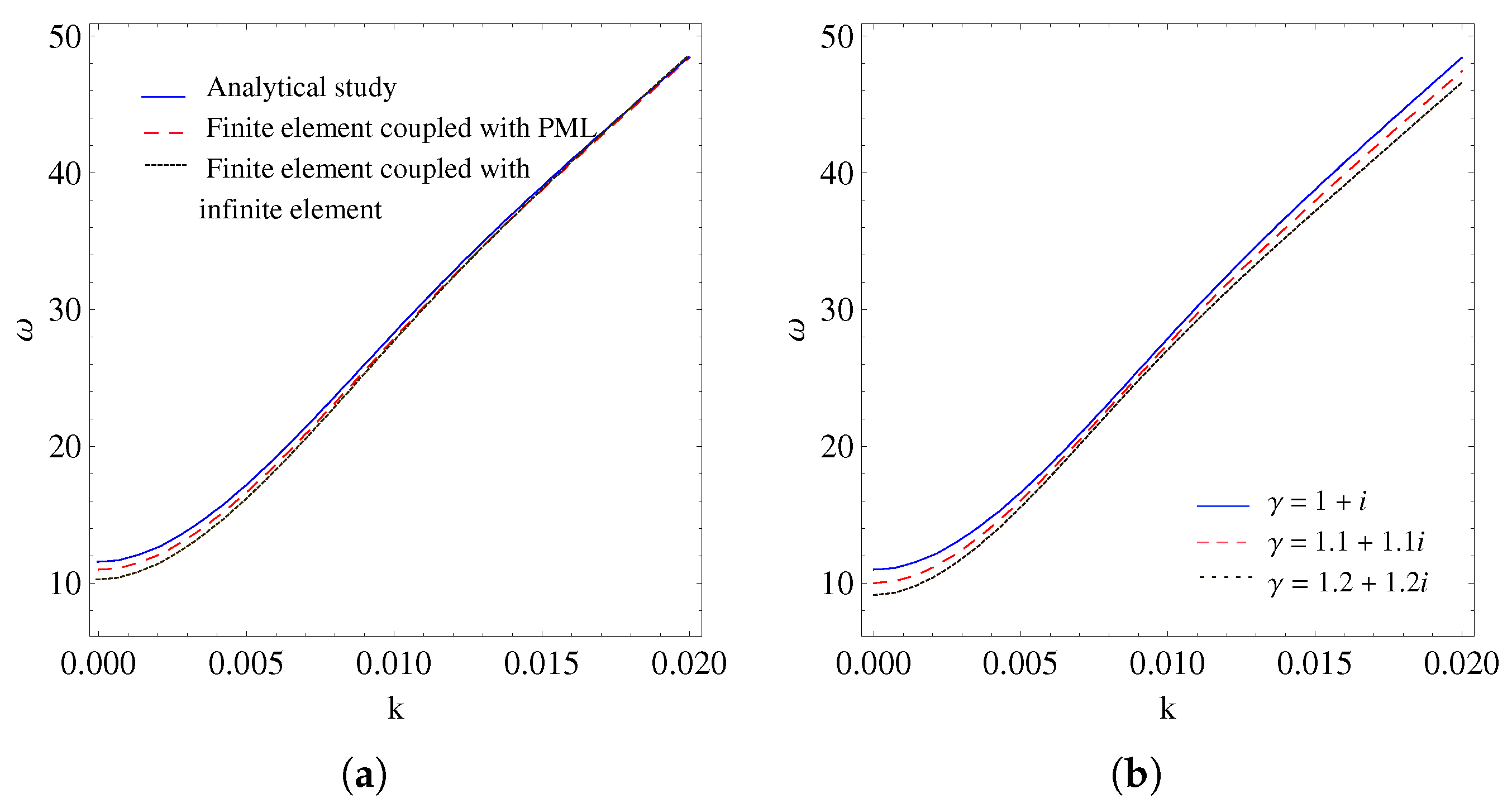
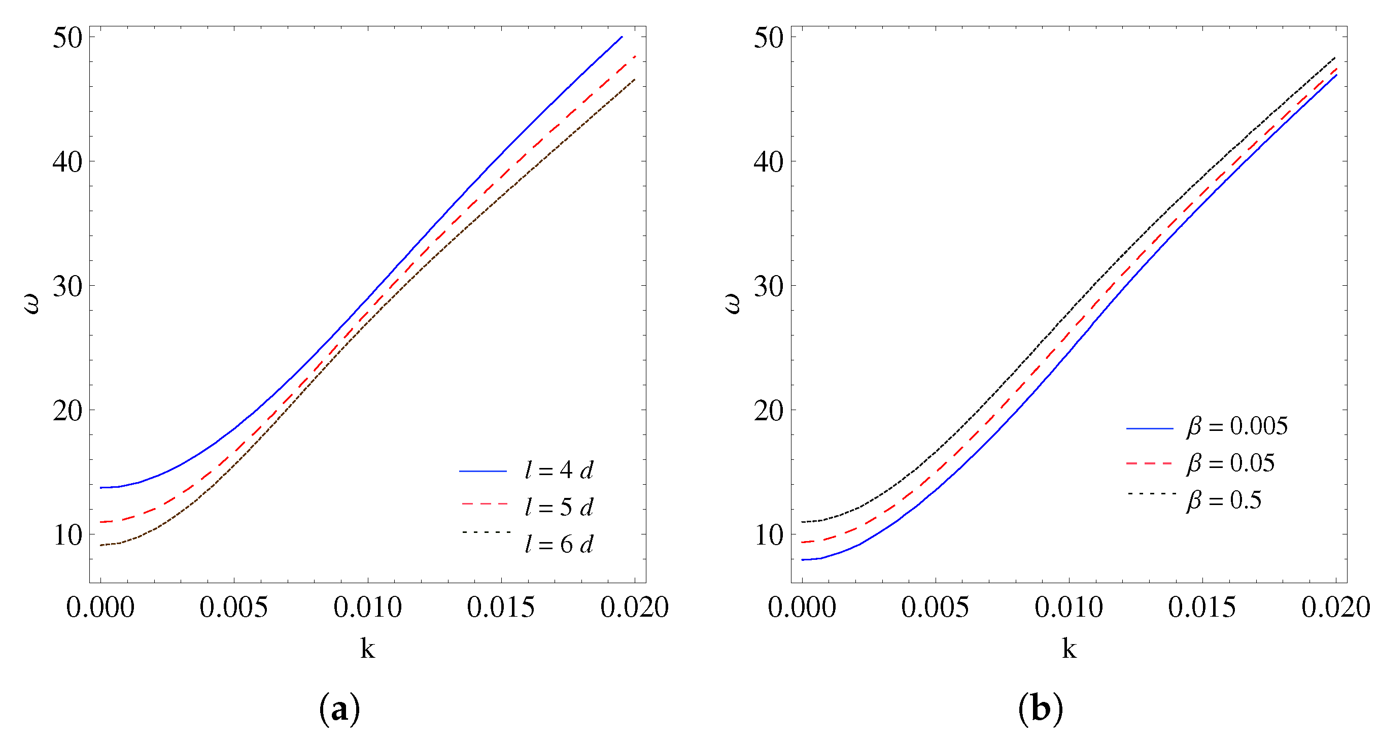
6. Numerical Results and Discussion

In this section, we examine the dispersion characteristics of SH waves. Our focus centers on a FGPHS with linear and quadratic gradient parameters. The dispersion analysis employs analytical methods, including the Wentzel–Kramers–Brillouin (WKB) approximation, alongside numerical techniques such as the finite element method (FEM). We also assess the influence of different perfectly matched layer (PML) functions, the in-homogeneity parameter, and structural length on dispersion behavior. A comparative evaluation of analytical and numerical results is provided. For clarity, the key material parameters of the FGPHS covering both linear and quadratic gradient variations are summarized in a dedicated

Table 1. The mechanical and electrical properties of PZT-5H ceramic.

Property	Symbol	Unit	Value
Elastic constant	$C_{44}$	$\left({10}^{10}{\mathrm{N}/\mathrm{m}}^2\right)$	2.3
Mass density	$\rho$	$\left({10}^3{\mathrm{kg}/\mathrm{m}}^3\right)$	7.5
Piezoelectric constant	$e_{15}$	${(\mathrm{C}/\mathrm{m}}^2)$	17
Dielectric constant	${\kappa }_{11}$	$\left({10}^{-10}\mathrm{F}/\mathrm{m}\right)$	277

.

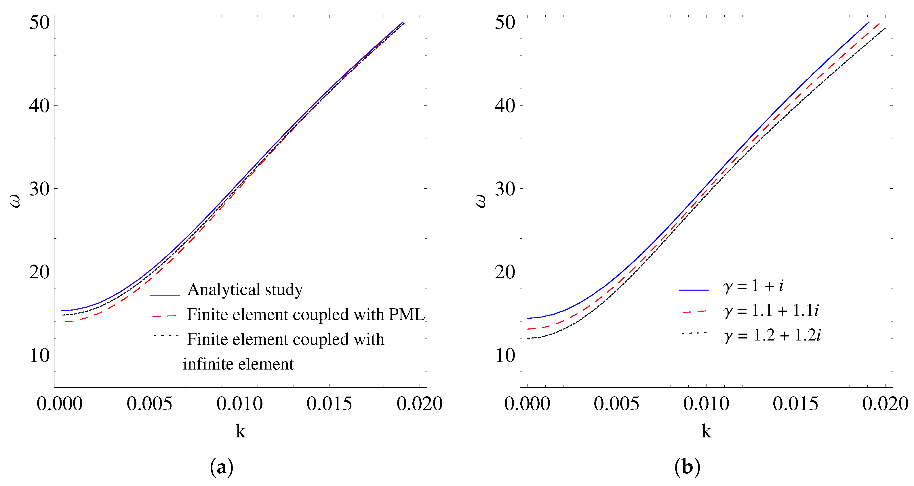
6.1. SAFE-PML Methodology

Certain assumptions were undertaken for numerical implementation of the SAFE-PML technique. They are provided as follows:

• The Gaussian 3-point quadrature method is utilized for numerical integration, enabling the efficient calculation of the stiffness matrix elements via Equation (45) and the mass matrix elements via Equation (46).

  $$\begin{array}{c}\hfill {\int }_{-1}^{1}f\left(\eta \right)=\sum _{i=1}^3{w}_{i}f\left({\eta }_i\right)\end{array}$$

  (83)
  The quadrature points are denoted by ${\eta }_i$, and the corresponding quadrature weights are represented by $w_i$, satisfying the following conditions:

  $${\eta }_1=-\sqrt{{\displaystyle \frac{3}{5}}},{\eta }_2=0,{\eta }_3=\sqrt{{\displaystyle \frac{3}{5}}},w_1={\displaystyle \frac{5}{9}},w_2={\displaystyle \frac{8}{9}},w_3={\displaystyle \frac{5}{9}}$$
• The Jacobian of the transformation in Equation (36) is determined to be half the length of the element. Thus, for element e corresponding to the FGPHS, we have $J_1={\displaystyle \frac{d}{2}}$, which is applied in Equations (40)–(43) and taking into account that $d=50$.
• The Gaussian 3-point quadrature formula, as defined in Equation (83), is utilized to compute the components of both the stiffness and mass matrices.

6.2. SAIFE Methodology

The following key assumptions are crucial for the effective numerical implementation of the SAIFE method:

• The finite element e, with a length of l, represents the bounded FGPHS. Additionally, to simulate the FGPHS, an infinite element is introduced, where the Jacobian $J_2$ of transformation Equation (44) is $J_2={\displaystyle \frac{2d}{{(1-s)}^2}}$, and it is employed in Equations (54)–(57) considering that $d=50$.
• Taking into account the $(1/r)$ decay outlined in Equation (53) and the propagation of SH waves in the half-space, it is assumed that $u_3={\varphi }_3=0$. As a result, Equation (44) reduces to a $3\times 3$ eigenvalue problem for $\omega$.
• The Gaussian 3-point quadrature formula, as defined in Equation (83), is utilized to compute the components of both the stiffness and mass matrices.

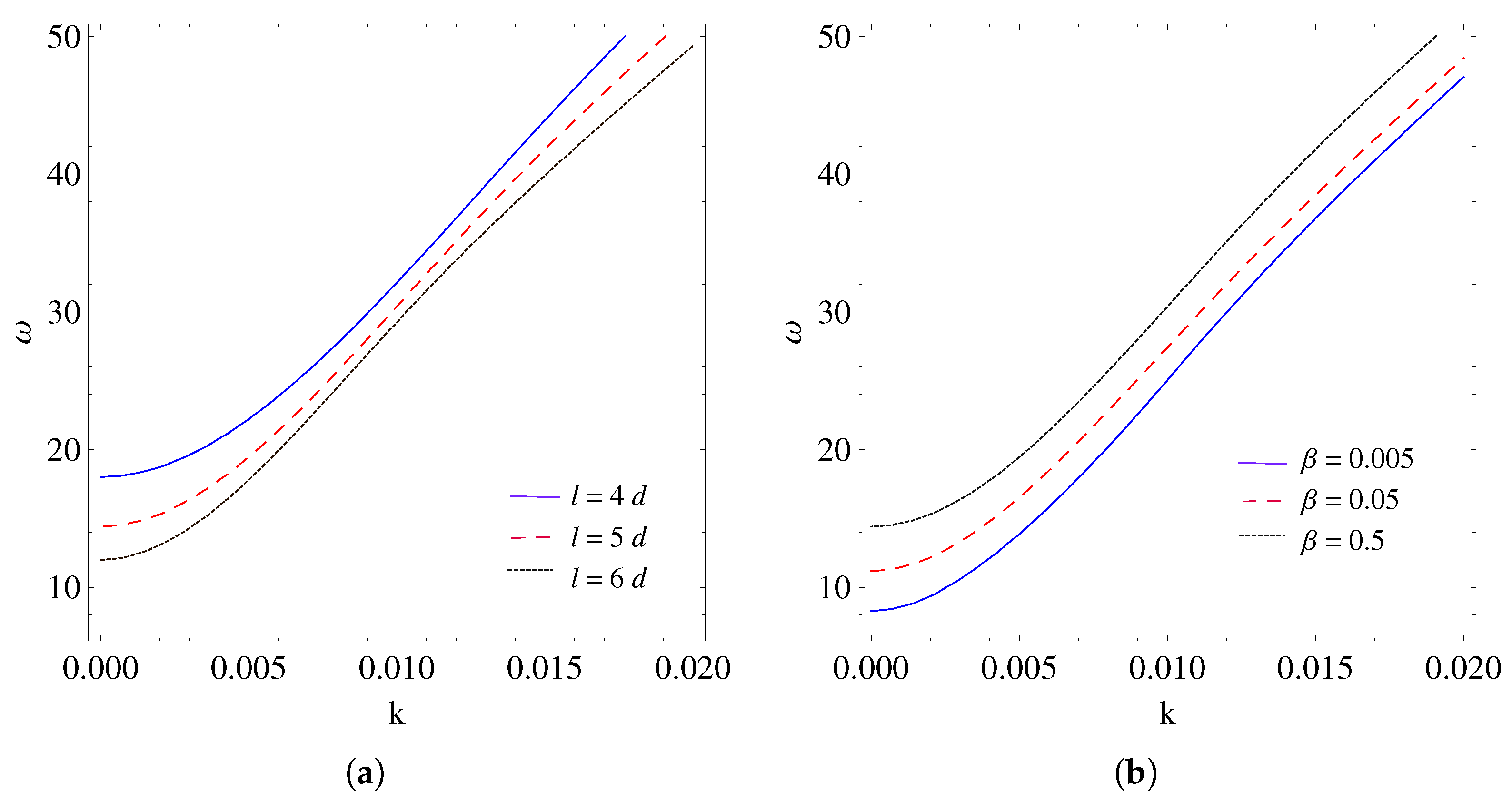
6.3. Linear Gradedness Parameter

This section presents an analysis of figures depicting the correlation between the frequency and wave number based on the dispersion relation, particularly highlighting the influence of the linear gradeness parameters. In materials exhibiting linear gradeness, the stiffness encountered by shear waves undergoes a steady alteration as they penetrate deeper. This leads to predictable outcomes, wherein the wave velocity, frequency, or wavelength shows a directly proportional change with depth. Figure 3a presents a comparative examination of the dispersion relation, specifically focusing on how frequency changes with wave number, using both analytical and numerical approaches. At low wave numbers, there is a slight divergence between the frequency curves, but as the wave number increases, they converge and closely resemble each other. The representation values of the complex stretching functions $\gamma$ are $1+i,1.1+1.1i,1.2+1.2i$ which are employed in the perfectly matched layer (PML) technique to simulate an absorbing boundary. These specific values were selected based on their effectiveness in attenuating outgoing waves while maintaining numerical stability. In the PML formulation, the real part controls coordinate scaling, and the imaginary part introduces damping. We chose this progression to evaluate the impact of increased absorption strength and found that these settings effectively minimized reflections without introducing instability or affecting the physical solution.

The results indicate a significant alignment between the numerical analysis using the perfectly matched layer (PML) and infinite element formulations and the analytical approach based on the WKB method. As shown in Figure 3b, an increase in the complex stretching function corresponds to a reduction in the frequency. This phenomenon occurs due to heightened energy dissipation or damping of high-frequency components within the waves. Figure 4a reveals that frequencies tend to rise as the in-homogeneity parameter decreases. This is because diminishing the in-homogeneity parameter reduces dispersion effects, enabling frequencies to increase due to a more uniform medium. Consequently, there is less variation in wave propagation speeds across different frequency components.

On the other hand, Figure 4b clearly shows the impact of varying PML lengths regarding the angular frequency of the SH waves. Shorter lengths of the PML result in a decrease in the damping effect of the boundary layer. Therefore, less energy is absorbed at the boundary, allowing more energy to propagate through the domain. This leads to a decrease in the angular frequency of the SH waves because more energy remains within the system, rather than being absorbed by the boundary layer.

6.4. Quadratic Gradedness Parameter

This section presents an analysis of figures depicting the correlation between the frequency and wave number based on the dispersion relation, particularly highlighting the influence of the quadratic gradeness parameters. Under quadratic gradeness, shear waves undergo a non-uniform adaptation in stiffness as they penetrate deeper. Initially, this adaptation progresses gradually, but it later intensifies or diminishes with increasing depth. Consequently, the wave dynamics become intricate, leading to fluctuations in wave velocity, frequency, or wavelength that diverge from a linear correlation with depth.

Figure 5a presents a comparative examination of the dispersion relation, specifically focusing on how frequency changes with wave number, using both analytical and numerical approaches. At low wave numbers, there is a slight divergence between the frequency curves, but as the wave number increases, they converge and closely resemble each other. The results indicate a significant correlation between the numerical analysis using the PML and infinite element formulations and the analytical approach based on the WKB method.

As shown in Figure 5b, frequency curves for various PML functions are presented. Consistent with previous observations, it is evident that the frequency decreases with an increase in the wave number. This trend can be attributed to heightened energy dissipation or damping of high-frequency components within the waves. We observed in Figure 6a that as the in-homogeneity parameter rises, the frequencies tend to increase. This is because higher in-homogeneity parameters have the potential to introduce dispersion effects, particularly noticeable at lower wave numbers. The dispersion effects cause the various frequency components of a wave to travel at distinct speeds, leading to variations in wave velocity that depend on frequency. Figure 6b demonstrates the impact of varying PML lengths regarding the angular frequency of the SH waves. Shorter lengths of the PML correspond to a weaker damping effect at the boundary. Consequently, less wave energy is absorbed, allowing more propagation throughout the domain. This results in a decrease in the angular frequency of SH waves, since more energy remains in the system rather than being absorbed by the boundary layer, which is especially evident for the case of the linear gradedness parameter.

7. Conclusions

This study comprehensively examined the propagation of transverse waves in a functionally graded piezoelastic half-space structure (FGPHS), characterized by linear and quadratic gradation in the material properties. Using an analytical approach with the WKB method, the dispersion relation for the homogeneous model was derived. Furthermore, two advanced numerical techniques—the SAFE-PML method and the SAIFE approach—were employed to gain deeper insights into the findings. A thorough analysis of the discretization process for both numerical methods was provided. The results indicate that an increase in wave number leads to a corresponding increase in the angular frequency of the transverse waves. This study also demonstrates that linear and quadratic gradedness parameters within the FGPHS influence variations in both the frequency and wave number.

Furthermore, the investigation reveals that the frequency of shear waves in the properties of these materials are shaped by a range of factors, covering PML function, the heterogeneity coefficient, and the length derived from the absorbing layer used in numerical simulations. Both the analytical WKB approach and the numerical SAFE-PML and SAIFE methods demonstrated good agreement by showing convergence of frequency curves as wave numbers increase for both linear and quadratic gradedness parameters. In addition, the complex stretching function, denoted as $\gamma$, has become a pivotal factor, affecting the frequency and wave number for both linear and quadratic gradedness parameters. At high wave numbers, a more complex stretching function decreases the frequency due to increased impedance or energy dissipation within the medium.

The results show that the frequency of transverse waves is significantly affected by the in-homogeneity parameter in both linear and quadratic graded materials. Notably, increasing the in-homogeneity parameter causes a rise in frequencies, especially at lower wave numbers. We found that the effect of different PML lengths on the angular frequency of transverse waves is consistent, regardless of whether the grading parameters are linear or quadratic. Finally, the results show that the longer PML lengths correspond to lower angular frequencies, ensuring effective absorption of outgoing waves.

References

1. Liu, G.R. Lamb waves in a functionally gradient material plate and its transient response, Part 1: Theory, Part 2: Calculation results. Trans. Jpn. Soc. Mech. Eng. 1991, 57, 131. [Google Scholar] [CrossRef]
2. Han, X.; Liu, G.R.; Xi, Z.C.; Lam, K.Y. Transient waves in a functionally graded cylinder. Int. J. Solids Struct. 2001, 38, 3021–3037. [Google Scholar] [CrossRef]
3. Han, X.; Liu, G.R.; Xi, Z.C.; Lam, K.Y. Characteristics of waves in a functionally graded cylinder. Int. J. Numer. Methods Eng. 2002, 53, 653–676. [Google Scholar] [CrossRef]
4. Liu, G.R.; Tani, J. SH surface waves in functionally gradient piezoelectric material plates. JSME Trans. 1992, 58, 504–507. [Google Scholar] [CrossRef]
5. Liu, G.R.; Tani, J. Surface waves in functionally gradient piezoelectric plates. J. Vib. Acoust. 1994, 116, 440–448. [Google Scholar] [CrossRef]
6. Han, X.; Liu, G.R. Effects of SH waves in a functionally graded plate. Mech. Res. Commun. 2002, 29, 327–338. [Google Scholar] [CrossRef]
7. Han, X.; Liu, G.R. Elastic waves in a functionally graded piezoelectric cylinder. Smart Mater. Struct. 2003, 12, 962. [Google Scholar] [CrossRef]
8. Li, X.Y.; Wang, Z.K.; Huang, S.H. Love waves in functionally graded piezoelectric materials. Int. J. Solids Struct. 2004, 41, 7309–7328. [Google Scholar] [CrossRef]
9. Chaudhary, S.; Sahu, S.A.; Singhal, A. Analytic model for Rayleigh wave propagation in piezoelectric layer overlaid orthotropic substratum. Acta Mech. 2017, 228, 495–529. [Google Scholar] [CrossRef]
10. Qian, Z.; Jin, F.; Wang, Z.; Kishimoto, K. Transverse surface waves on a piezoelectric material carrying a functionally graded layer of finite thickness. Int. J. Eng. Sci. 2007, 45, 455–466. [Google Scholar] [CrossRef]
11. Chaki, M.S.; Bravo-Castillero, J. A mathematical analysis of anti-plane surface wave in a magneto-electro-elastic layered structure with non-perfect and locally perturbed interface. Eur. J. Mech. A/Solids 2023, 97, 104820. [Google Scholar] [CrossRef]
12. Qian, Z.; Jin, F.; Wang, Z.; Kishimoto, K. Love waves propagation in a piezoelectric layered structure with initial stresses. Acta Mech. 2004, 171, 41–57. [Google Scholar] [CrossRef]
13. Jin, F.; Qian, Z.; Wang, Z.; Kishimoto, K. Propagation behavior of Love waves in a piezoelectric layered structure with in-homogeneous initial stress. Smart Mater. Struct. 2005, 14, 515. [Google Scholar] [CrossRef]
14. Han, X.; Liu, G.R.; Lam, K.Y. Transient waves in plates of functionally graded materials. Int. J. Numer. Methods Eng. 2001, 52, 51–865. [Google Scholar] [CrossRef]
15. Singh, R.; Prasad, S. The propagation behavior of SH surface waves in a semi-infinite magneto-electro-elastic solid with the periodically gold strips. Mater. Today Commun. 2023, 2023, 106266. [Google Scholar] [CrossRef]
16. Akshaya, A.; Kumar, S.; Hemalatha, K. Transference of SH-Waves in Two Different Functionally Graded Half-Spaces. Mech. Solids 2024, 13, 1–22. [Google Scholar] [CrossRef]
17. Hemalatha, K.; Kumar, S. Propagation of SH Wave in a Rotating Functionally Graded Magneto-Electro-Elastic Structure with Imperfect Interfac. J. Vib. Eng. Technol. 2024, 19, 1–5. [Google Scholar]
18. Akshaya, A.; Kumar, S.; Hemalatha, K. Behaviour of Transverse Wave at an Imperfectly Corrugated Interface of a Functionally Graded Structure. Phys. Wave Phenom. 2024, 32, 117–134. [Google Scholar] [CrossRef]
19. Akshaya, A.; Kumar, S.; Hemalatha, K. Propagation of Shear Horizontal Wave at Magneto-Electro-Elastic Structure Subjected to Mechanically Imperfect Interface. Mech. Adv. Compos. Struct. 2025, 12, 97–114. [Google Scholar]
20. Hemalatha, K.; Kumar, S.; Akshaya, A. Influence of corrugation on SH wave propagation in rotating and initially stressed functionally graded magneto-electro-elastic substrate. Geomech. Eng. 2025, 40, 79. [Google Scholar]
21. Fröman, N.; Fröman, P.O. Physical Problems Solved by the Phase-Integral Method; Cambridge University Press: Cambridge, UK, 2002. [Google Scholar]
22. Cerveny, V.; Ravindra, R. Theory of Seismic Head Waves; University of Toronto Press: Toronto, ON, Canada, 2017. [Google Scholar]
23. Kumar, P.; Mahanty, M.; Chattopadhyay, A.; Singh, A.K. Effect of interfacial imperfection on shear wave propagation in a piezoelectric composite structure: Wentzel–Kramers–Brillouin asymptotic approach. J. Intell. Mater. Syst. Struct. 2019, 30, 2789–2807. [Google Scholar] [CrossRef]
24. Morsbøl, J.O.; Sorokin, S.V.; Peake, N. A WKB approximation of elastic waves travelling on a shell of revolution. J. Sound Vib. 2016, 375, 162–186. [Google Scholar] [CrossRef]
25. Liu, J.; Wang, Z.K. The propagation behavior of Love waves in a functionally graded layered piezoelectric structure. Smart Mater. Struct. 2004, 14, 137. [Google Scholar] [CrossRef]
26. Du, J.; Jin, X.; Wang, J.; Xian, K. Love wave propagation in functionally graded piezoelectric material layer. Ultrasonics 2007, 46, 13–22. [Google Scholar] [CrossRef]
27. Hua, L.I.U.; Yang, J.L.; Liu, K.X. Love waves in layered graded composite structures with imperfectly bonded interface. Chin. J. Aeronaut. 2007, 20, 210–214. [Google Scholar]
28. Holubets, T.; Terletskiy, R.; Yuzevych, V. The Analytical Expressions to Describe Wave Propagation and Heat Release During Microwave Treatment of Porous in-homogeneous Plate Based on the WKB Solution Model. Adv. Mater. Sci. 2023, 23, 69–81. [Google Scholar] [CrossRef]
29. Qian, Z.H.; Jin, F.; Kishimoto, K.; Lu, T. Propagation behavior of Love waves in a functionally graded half-space with initial stress. Int. J. Solids Struct. 2009, 46, 1354–1361. [Google Scholar] [CrossRef]
30. Roy, T.; Manikandan, P.; Chakraborty, D. Improved shell finite element for piezothermoelastic analysis of smart fiber reinforced composite structures. Finite Elem. Anal. Des. 2010, 46, 710–720. [Google Scholar] [CrossRef]
31. de León, L.B.; Camacho-Montes, H.; Espinosa-Almeyda, Y.; Otero, J.A.; Rodríguez-Ramos, R.; López-Realpozo, J.C.; Sabina, F.J. Semi-analytic finite element method applied to short-fiber-reinforced piezoelectric composites. Contin. Mech. Thermodyn. 2021, 33, 1957–1978. [Google Scholar] [CrossRef]
32. Basu, U.; Chopra, A.K. Perfectly matched layers for time-harmonic elastodynamics of unbounded domains: theory and finite-element implementation. Comput. Methods Appl. Mech. Eng. 2003, 192, 1337–1375. [Google Scholar] [CrossRef]
33. Zeng, Y.; He, J.; Liu, Q. The application of the perfectly matched layer in numerical modeling of wave propagation in poroelastic media. Geophysics 2001, 66, 1258–1266. [Google Scholar] [CrossRef]
34. Pelat, A.; Felix, S.; Pagneux, V. A coupled modal-finite element method for the wave propagation modeling in irregular open waveguides. J. Acoust. Soc. Am. 2011, 129, 1240–1249. [Google Scholar] [CrossRef]
35. Harari, I.; Albocher, U. Studies of FE/PML for exterior problems of time-harmonic elastic waves. Comput. Methods Appl. Mech. Eng. 2006, 195, 3854–3879. [Google Scholar] [CrossRef]
36. Bermúdez, A.; Hervella-Nieto, L.; Prieto, A.; Rodrı, R. An optimal perfectly matched layer with unbounded absorbing function for time-harmonic acoustic scattering problems. J. Comput. Phys. 2007, 223, 469–488. [Google Scholar] [CrossRef]
37. Marques, J.M.M.C.; Owen, D.R.J. Infinite elements in quasi-static materially nonlinear problems. Comput. Struct. 1984, 18, 739–751. [Google Scholar] [CrossRef]
38. Zhao, C.; Valliappan, S. A dynamic infinite element for three-dimensional infinite-domain wave problems. Int. J. Numer. Methods Eng. 1993, 36, 2567–2580. [Google Scholar] [CrossRef]
39. Khalili, N.; Valliappan, S.; Yazdi, J.T.; Yazdchi, M. 1D infinite element for dynamic problems in saturated porous media. Commun. Numer. Methods Eng. 1997, 13, 727–738. [Google Scholar] [CrossRef]
40. Khalili, N.; Yazdchi, M.; Valliappan, S. Wave propagation analysis of two-phase saturated porous media using coupled finite–infinite element method. Soil Dyn. Earthq. Eng. 1999, 18, 533–553. [Google Scholar] [CrossRef]
41. Zhao, C. Coupled method of finite and dynamic infinite elements for simulating wave propagation in elastic solids involving infinite domains. Sci. China Technol. Sci. 2010, 53, 1678–1687. [Google Scholar] [CrossRef]
42. Hao, X.; Qingsheng, C.; Bingjian, Z. Directional interpolation infinite element for dynamic problems in saturated porous media. Earthq. Eng. Eng. Vib. 2020, 19, 625–635. [Google Scholar] [CrossRef]
43. Su, J.; Wang, Y. Equivalent dynamic infinite element for soil–structure interaction. Finite Elem. Anal. Des. 2013, 63, 1–7. [Google Scholar] [CrossRef]
44. Lynn, P.P.; Hadid, H.A. Infinite elements with 1/rn type decay. Int. J. Numer. Methods Eng. 1981, 17, 347–355. [Google Scholar] [CrossRef]
Figure 1. The global degrees-of-freedom representation of the 3-noded elements.
Mathematics 13 02131 g001
Figure 2. Infinite element representation of FGPHS.
Mathematics 13 02131 g002
Figure 3. (a) Comparison of frequency curves derived from the analytical method, SAFE-PML method, and infinite element method with a ( 1 / r ) decay type for the linear gradation parameter and (b) angular frequency vs. wave number for varying the γ and linear gradedness parameter.
Mathematics 13 02131 g003
Figure 4. The angular frequency vs. wave number for varying (a) β and linear gradedness parameters and (b) l and linear gradedness parameters.
Mathematics 13 02131 g004
Figure 5. (a) Comparison of frequency curves from the analytical, SAFE-PML, and infinite element methods with ( 1 / r ) decay for quadratic grading and (b) the angular frequency vs. the wave number for varying γ and quadratic gradedness parameter values.
Mathematics 13 02131 g005
Figure 6. The angular frequency vs. wave number for varying (a) β and linear gradedness parameter and (b) l and linear gradedness parameter values.
Mathematics 13 02131 g006