Asymptotic Analysis of Poverty Dynamics via Feller Semigroups

Abstract

Poverty is a multifaceted phenomenon impacting millions globally, defined by a deficiency in both material and immaterial resources, which consequently restricts access to satisfactory living conditions. Comprehensive poverty analysis can be accomplished through the application of mathematical and modeling techniques, which are useful in understanding and predicting poverty trends. These models, which often incorporate principles from economics, stochastic processes, and dynamic systems, enable the assessment of the factors influencing poverty and the effectiveness of public policies in alleviating it. This paper introduces a mathematical compartmental model to investigate poverty within a population ($\psi \left(t\right)$), considering the effects of immigration, crime, and incarceration. The model aims to elucidate the interconnections between these factors and their combined impact on poverty levels. We begin the study by ensuring the mathematical validity of the model by demonstrating the uniqueness of a positive solution. Next, it is shown that under specific conditions, the probability of poverty persistence approaches certainty. Conversely, conditions leading to an exponential reduction in poverty are identified. Additionally, the semigroup associated with our model is proven to possess the Feller property, and its distribution has a unique invariant measure. To confirm and validate these theoretical results, interesting numerical simulations are performed.

1. Introduction

Poverty is a socioeconomic condition marked by insufficient financial resources and material possessions, resulting in the inability to attain adequate living standards and opportunities for human growth, including access to nourishment, shelter, medical care, education, suitable employment, and community involvement [1]. Despite the improvement in the standard of living and the increase in the economic growth rate, almost 700 million people live below the extreme poverty line of 2.15 dollars per day around the world [2].

Understanding and addressing poverty require rigorous analysis, as it remains one of the most pressing and complex socioeconomic challenges of our time. Poverty analysis is crucial not only for identifying its root causes and affected populations but also for designing effective interventions. In this context, mathematical modeling emerges as a powerful tool for examining poverty dynamics and their broader societal impacts. Specifically, compartmental models offer a robust analytical framework that enables researchers and policymakers to simulate the spread of poverty, evaluate the effectiveness of public policies, forecast future scenarios, and pinpoint the most vulnerable segments of the population [3]. These models provide structured, evidence-based insights that are essential for crafting informed and impactful strategies to alleviate poverty. In [4], the authors proposed a compartmental mathematical model to analyze the dynamics of poverty and prostitution in Nigeria. This model divides the total population into five classes: the non-poor, the poor, prostitutes, the infected prostitute, and those undergoing rehabilitation. Through the stability analysis of the model’s equilibrium points, the authors inferred that rigorous and effective government intervention would lead to a faster decline in the poverty rate, consequently resulting in a gradual reduction in the number of individuals involved in prostitution. In this context, government intervention encompasses social policies and governmental programs designed to enhance the economic conditions of economically disadvantaged groups. These programs include vocational training, employment, education opportunities, and the promotion of moral values and self-preservation through religious teachings.

Mansour et al. [5] investigated the correlation between corruption and poverty dynamics using a statistical approach. They sourced data on the corruption index from Transparency International and poverty rates in Yemen from household budget surveys and annual publications by the Central Bureau of Statistics (2003–2022). Employing a linear model and the Eviews program, they analyzed these metrics throughout the study period and presented estimations of poverty rates for 2023 and 2024. Complementing this statistical analysis, the authors developed an analytical framework using Caputo fractional derivatives to model the relationship between poverty and corruption, determining the equilibrium points, basic reproduction number, and positive solution. Subsequently, they examined the solution’s uniqueness and Ulam–Hyers stability using Banach’s fixed point theorem for their proposed model.

Poverty also negatively impacts the health status of societies. The association between poverty and the spread of diseases was examined in [6] to evaluate the ramifications of poverty on yaws eradication efforts. Yaws, a tropical infection affecting the bones and skin, is caused by the spirochete bacterium Treponema pallidum pertenue (for further details, see [7,8]). The authors developed a deterministic differential systems model to analyze the transmission of yaws among children from different socioeconomic strata, specifically, the poor and the rich. They identified thresholds and analyzed the stability. The findings of this theoretical analysis suggest that the eradication of yaws remains challenging when the demographic composition of the community is skewed toward children from economically disadvantaged families. Addressing issues such as overcrowding, inadequate sanitation, and pervasive poverty is crucial to prevent the resurgence of yaws.

In 1968, Gary Becker introduced an economic theory of criminal behavior in his publication Crime and Punishment: An Economic Approach, positing that individuals engage in criminal activities exclusively when the perceived advantages outweigh the associated costs. Consequently, individuals experiencing impoverished conditions exhibit a heightened propensity for criminal involvement in comparison to their more economically stable counterparts [9]. Hence, a direct link can be observed between poverty and criminal tendencies.

Several interesting studies have explored the dynamics of crime by compartmental models based on deterministic differential systems. Achieving a stability analysis for a deterministic differential system, Misra hypothesized that the rise in criminal individuals within society can be attributed to either the migration of criminals from external locales into the focal region or through the interactions between individuals involved in criminal activities and those with inclinations toward criminal behavior. Therefore, the police forces should discourage criminal activity by reducing the inflow of criminals through immigration [10]. In another study, Haiyun Zhao and his co-authors constructed a model that connects poverty and crime [11]. The circulation of individuals oscillates among five compartments: those comprising non-poor individuals, individuals living in poverty, individuals with a criminal record, incarcerated individuals, and individuals who have transitioned from either incarceration or poverty. In addition to assessing the stability of the acquired model, the authors sought to identify additional low-cost crime-fighting strategies. They examined the potential for crime control through governmental interventions and concluded that such measures can be effective without incurring additional financial costs, even in the absence of intervention and rehabilitation programs. Assuming that the complete eradication of crime is unachievable, the authors also demonstrate the existence of an optimal value for parameters ${\mathfrak{K}}_1$ and ${\mathfrak{K}}_2$, denoting the rate at which individuals move from poverty to recovery either from incarceration or poverty and the rate of incarceration, respectively. These two parameters minimize the cost of fighting crime, defined by a cost function subject to an optimization calculation.

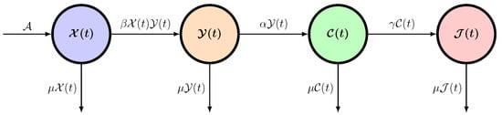
Building upon the detailed discussion above, we aim to formulate a mathematical model that elucidates the dynamics of urban poverty in relation to rural-to-urban migration. The total population is categorized into four distinct classes: the criminal class ($\mathcal{C}$) comprising individuals who have committed crimes, the class of incarcerated individuals ($\mathcal{J}$), the impoverished class ($\mathcal{Y}$), and the vulnerable category ($\mathcal{X}$), which includes individuals who are not currently poor but are at risk of poverty due to various factors, such as wars, financial and economic crises, serious inflation, and health crises, like the COVID-19 pandemic, leading to widespread unemployment globally (for a more in-depth understanding of the causes of poverty, we refer readers to the books of some of the most prominent economists [12,13,14,15,16]). Let $\mathcal{A}$ be the number of individuals from rural areas who are likely to become impoverished. The symbol $\mu$ denotes the death rate, while $\beta$ signifies the interdependence between the susceptible class ($\mathcal{X}$) and the impoverished class ($\mathcal{Y}$). We can also define $\beta$ quite simply as the poverty rate in the total population ($\psi =\mathcal{X}+\mathcal{Y}+\mathcal{C}+\mathcal{J}$). Another critical assumption is that an individual from the impoverished class ($\mathcal{Y}$) may commit a crime and transition to the criminal class ($\mathcal{C}$) with a probability of $\alpha$. The term $\gamma \mathcal{C}$ represents the number of criminals sentenced to prison. With these assumptions in mind, the interrelation among poverty, crime, and immigration is governed by the following system of four ordinary differential equations:

$$\begin{array}{c}\hfill \left\{\begin{array}{cc}d\mathcal{X}\left(t\right)=\hfill & \left(\mathcal{A}-\beta \mathcal{X}\left(t\right)\mathcal{Y}\left(t\right)-\mu \mathcal{X}\left(t\right)\right)dt,\hfill \\ d\mathcal{Y}\left(t\right)=\hfill & \left(\beta \mathcal{X}\left(t\right)\mathcal{Y}\left(t\right)-\mu \mathcal{Y}\left(t\right)-\alpha \mathcal{Y}\left(t\right)\right)dt,\hfill \\ d\mathcal{C}\left(t\right)=\hfill & \left(-\mu \mathcal{C}\left(t\right)+\alpha \mathcal{Y}\left(t\right)-\gamma \mathcal{C}\left(t\right)\right)dt,\hfill \\ d\mathcal{J}\left(t\right)=\hfill & \left(-\mu \mathcal{J}\left(t\right)+\gamma \mathcal{C}\left(t\right)\right)dt.\hfill \end{array}\right.\end{array}$$

(1)

The flowchart of the deterministic model is given in Figure 1. The deterministic model (1) has two equilibrium states: ${\mathsf{\Sigma }}_1=\left({\mathcal{X}}_0,{\mathcal{Y}}_0,{\mathcal{C}}_0,{\mathcal{J}}_0\right)=\left({\displaystyle \frac{\mathcal{A}}{\mu }},0,0,0\right)$ and ${\mathsf{\Sigma }}_2=\left({\mathcal{X}}_{*},{\mathcal{Y}}_{*},{\mathcal{C}}_{*},{\mathcal{J}}_{*}\right)=\left({\displaystyle \frac{\mu +\alpha }{\beta }},{\displaystyle \frac{\mu }{\beta }}(\mathcal{R}-1),{\displaystyle \frac{\alpha }{\mu +\gamma }}{\mathcal{Y}}_{*},{\displaystyle \frac{\gamma \alpha }{\mu (\mu +\gamma )}}{\mathcal{Y}}_{*}\right)$, where $\mathcal{R}={\displaystyle \frac{\beta \mathcal{A}}{\mu (\mu +\alpha )}}$. To study the stability of these equilibrium states, we employ the Jacobian matrix of (1) defined by

$$\mathsf{\Xi }\left(\mathcal{X},\mathcal{Y},\mathcal{C},\mathcal{J}\right)=\left(\begin{array}{cccc}-\beta \mathcal{Y}-\mu & -\beta \mathcal{X}& 0& 0\\ \beta \mathcal{Y}& \beta \mathcal{X}-(\mu +\alpha )& 0& 0\\ 0& \alpha & -(\mu +\gamma )& 0\\ 0& 0& \gamma & -\mu \end{array}\right).$$

Figure 1. Flowchart of the deterministic model (1).

At the first equilibrium state, the matrix $\mathsf{\Xi }$ has three eigenvalues: $-\mu$, $-(\mu +\alpha )$, and ${\displaystyle \frac{\beta \mathcal{A}}{\mu }}-(\mu +\alpha )$. Then, the state $\left({\mathcal{X}}_0,{\mathcal{Y}}_0,{\mathcal{C}}_0,{\mathcal{J}}_0\right)$ is locally asymptotically stable if $\mathcal{R}<1$.

Regarding the second equilibrium point, the characteristic polynomial of its corresponding Jacobian is

$$\left(\mu +\gamma +X\right)\left(\mu +X\right)\left(X^2+\mu \mathcal{R}X+\mu (\mu +\alpha )(\mathcal{R}-1)\right),\mathrm{where}\mathrm{X}\mathrm{is}\mathrm{its}\mathrm{root}.$$

Bearing in mind the Routh–Hurwitz stability criterion [17], the roots of the polynomial $X^2+\mu \mathcal{R}X+\mu (\mu +\alpha )(\mathcal{R}-1)$ are all negative if $\mathcal{R}>1$, which implies that the equilibrium $\left({\mathcal{X}}_{*},{\mathcal{Y}}_{*},{\mathcal{C}}_{*},{\mathcal{J}}_{*}\right)$ is locally asymptotically stable.

Numerous debates have emerged regarding the limitations of deterministic mathematical models in forecasting the behaviors of dynamic systems in environments characterized by complexity and stochasticity. In the work by Gleick [18], the concept of chaos theory is introduced, highlighting how minute variations in the initial conditions can lead to significantly divergent outcomes, thereby challenging the reliability of deterministic models in predicting future events. Similarly, Nassim Nicholas Taleb explored the substantial impacts of rare and unpredictable events, known as Black Swans, on financial markets and various complex systems, underscoring the limitations of deterministic models in accounting for extreme randomness [19]. Melanie Mitchell’s research [20] provides a comprehensive examination of complexity science, illustrating the inadequacies of traditional deterministic models in capturing the emergent behaviors and intricate interactions that characterize complex systems. In a related vein, Kevin Kelly argued that deterministic models have limited efficacy in forecasting the behaviors of self-organizing systems, such as biological organisms, as well as technological and social structures [21]. Mathematically, we follow the methodology outlined in [22,23,24,25,26,27] to introduce a stochastic component to the system (1) by adding rapidly fluctuating random terms, ${\delta }_1\left(t\right)$ and ${\delta }_2\left(t\right)$, to the parameters $\beta$ and $\mu$. This can be achieved by replacing $\beta dt$ with $\beta dt+{\delta }_1\left(t\right)dt$ and $\mu dt$ with $\mu dt+{\delta }_2\left(t\right)dt$ in the system (1). According to the central limit theorem [28], the random term ${\delta }_i\left(t\right)dt(i=1,2)$ can be approximated by a normal distribution with a zero mean and variance ${\sigma }_i^{2}dt>0(i=1,2)$. Considering the possibility of a correlation between the random terms ${\delta }_i\left(t\right)dt$, we represent them using one-dimensional Brownian motions, $\mathcal{B}i\left(t\right)$, such that $\delta i\left(t\right)dt={\sigma }_{i}d{\mathcal{B}}_i\left(t\right)$ for $i=1,2$. These Brownian motions are defined in a filtered probability space, $\left(\mathsf{\Omega },{\left({\mathcal{F}}_t\right)}_{t\ge 0},\mathbb{P}\right)$, accompanied by a filtration that conforms to the usual criteria. Therefore, we arrive at the following stochastic counterpart of the deterministic model (1):

$$\begin{array}{c}\hfill \left\{\begin{array}{cc}d\mathcal{X}\left(t\right)=\hfill & \left(\mathcal{A}-\beta \mathcal{X}\left(t\right)\mathcal{Y}\left(t\right)-\mu \mathcal{X}\left(t\right)\right)dt-{\sigma }_1\mathcal{X}\left(t\right)\mathcal{Y}\left(t\right)d{\mathcal{B}}_1\left(t\right)-{\sigma }_2\mathcal{X}\left(t\right)d{\mathcal{B}}_2\left(t\right),\hfill \\ d\mathcal{Y}\left(t\right)=\hfill & \left(\beta \mathcal{X}\left(t\right)\mathcal{Y}\left(t\right)-\mu \mathcal{Y}\left(t\right)-\alpha \mathcal{Y}\left(t\right)\right)dt+{\sigma }_1\mathcal{X}\left(t\right)\mathcal{Y}\left(t\right)d{\mathcal{B}}_1\left(t\right)-{\sigma }_2\mathcal{Y}\left(t\right)d{\mathcal{B}}_2\left(t\right),\hfill \\ d\mathcal{C}\left(t\right)=\hfill & \left(-\mu \mathcal{C}\left(t\right)+\alpha \mathcal{Y}\left(t\right)-\gamma \mathcal{C}\left(t\right)\right)dt-{\sigma }_2\mathcal{C}\left(t\right)d{\mathcal{B}}_2\left(t\right),\hfill \\ d\mathcal{J}\left(t\right)=\hfill & \left(-\mu \mathcal{J}\left(t\right)+\gamma \mathcal{C}\left(t\right)\right)dt-{\sigma }_2\mathcal{J}\left(t\right)d{\mathcal{B}}_2\left(t\right).\hfill \end{array}\right.\end{array}$$

(2)

For the convenience of the readers, we provide the following glossary of abbreviations and symbols utilized throughout this paper:

$$\begin{array}{cc}\hfill {\mathbb{R}}_{+}:& \mathrm{the}\mathrm{set}\mathrm{comprising}\mathrm{all}\mathrm{the}\mathrm{nonnegative}\mathrm{real}\mathrm{numbers}\hfill \\ \hfill {\mathbb{R}}_{+}^n:& =\{(x_1,\dots ,x_n):x_i>0,i=1,\dots ,n\},\mathrm{such}\mathrm{that}\mathrm{n}\mathrm{is}\mathrm{a}\mathrm{positive}\mathrm{integer}\mathrm{number}\hfill \\ \hfill \mathbb{E}\left(X\right):& \mathrm{the}\mathrm{expectation}\mathrm{of}\mathrm{the}\mathrm{random}\mathrm{variable}\mathrm{X}\hfill \\ \hfill ⟨Q\left(t\right)⟩:& =t^{-1}{\int }_0^{t}Q\left(u\right)du,\mathrm{where}\mathrm{Q}\mathrm{is}\mathrm{a}\mathrm{continuous}\mathrm{function}\hfill \\ \hfill a.s.:& \mathrm{almost}\mathrm{surely}\mathrm{or}\mathrm{with}\mathrm{a}\mathrm{probability}\mathrm{of}\mathrm{one}\hfill \\ \hfill \mathbb{P}:& \mathrm{the}\mathrm{probability}\mathrm{measure}\hfill \\ \hfill {\mathbf{1}}_{\mathcal{D}}:& \mathrm{the}\mathrm{indicator}\mathrm{function}\mathrm{of}\mathrm{a}\mathrm{set}\mathcal{D}\hfill \\ \hfill {\mathsf{\Delta }}_1:& =\{(\mathcal{X},\mathcal{Y})\in {\mathbb{R}}_{+}^2:\mathcal{X}\ge a\mathrm{and}\mathcal{Y}\ge a\}\hfill \\ \hfill {\mathsf{\Delta }}_2:& =\{\mathcal{X}\in {\mathbb{R}}_{+}:\mathcal{X}<a\}\hfill \\ \hfill {\mathsf{\Delta }}_3:& =\{\mathcal{Y}\in {\mathbb{R}}_{+}:\mathcal{Y}<a\}\hfill \\ \hfill {\mathsf{\Delta }}_4:& =\{(\mathcal{X},\mathcal{Y})\in {\mathbb{R}}_{+}^2:\mathcal{X}>b\mathrm{or}\mathcal{Y}>b\}\hfill \\ \hfill \mathsf{\Delta }:& =\{(\mathcal{X},\mathcal{Y})\in {\mathbb{R}}_{+}^2:a\le \mathcal{X}\le b\mathrm{and}a\le \mathcal{Y}\le b\},\mathrm{where}\mathrm{a}\mathrm{and}\mathrm{b}\mathrm{are}\mathrm{positive}\hfill \\ \hfill & \mathrm{numbers}\mathrm{to}\mathrm{be}\mathrm{specified}\mathrm{later}\hfill \\ \hfill \mathcal{L}& \mathrm{is}\mathrm{the}\mathrm{It}ô\mathrm{infinitesimal}\mathrm{generator}.\mathrm{For}\mathrm{a}\mathrm{diffusion}\mathrm{process},\hfill \\ \hfill & d{X}_t=H_1(X_t,t)dt+H_2(X_t,t)d{W}_t,\mathrm{where}{W}_t\mathrm{is}\mathrm{a}\mathrm{Brownian}\mathrm{motion}.\mathrm{If}\mathcal{L}\mathrm{acts}\mathrm{on}\hfill \\ \hfill & \mathrm{a}\text{twice-differentiable}\mathrm{function},F(X_t,t),\mathrm{we}\mathrm{get}\hfill \\ \hfill & \mathcal{L}F(x,t)={\displaystyle \frac{\partial F}{\partial t}}+H_1(x,t){\displaystyle \frac{\partial F}{\partial x}}+0.5H_2^2(x,t){\displaystyle \frac{{\partial }^{2}F}{\partial x^2}}.\hfill \end{array}$$

This paper represents the first study to employ stochastic mathematical methods to analyze poverty dynamics within a population. The subsequent sections of this article are organized as follows: Initially, in Section 2, we establish the existence of a global positive solution for our novel stochastic model. Following this, Section 3 examines the mathematical and statistical characteristics of the stochastic process ($\psi \left(t\right)$), providing insights into its behavior. Section 4 is then dedicated to deriving sufficient conditions that promote the prevalence and eradication of poverty within this framework. Continuing further, Section 5 utilizes the theory of stochastic semigroups to determine the conditions under which the model (2) achieves a stationary distribution, a contribution we consider to be the first application of such techniques to the study of poverty dynamics. Finally, Section 6 presents numerical simulations that serve to validate and illustrate our theoretical results.

2. The Well-Posedness of the Model

Theorem 1.

For any initial data $\mathcal{X}\left(0\right)>0,\mathcal{Y}\left(0\right)>0,\mathcal{C}\left(0\right)>0,\mathrm{and}\mathcal{J}\left(0\right)>0$, the model (2) has a global solution $(\mathcal{X}\left(t\right),\mathcal{Y}\left(t\right),\mathcal{C}\left(t\right),\mathcal{J}\left(t\right))\in {\mathbb{R}}_{+}^4$ for all $t>0$ almost surely.

Proof. 

Since the coefficients of the model (2) meet the requirements of the local Lipschitz conditions, for any initial data $(\mathcal{X}\left(0\right),\mathcal{Y}\left(0\right),\mathcal{C}\left(0\right),\mathcal{J}\left(0\right))\in {\mathbb{R}}_{+}^4$, there is a unique positive local solution $Z\left(t\right)=\left(\mathcal{X}\right(t),\mathcal{Y}(t),\mathcal{C}(t),\mathcal{J}(t\left)\right)$ in $[0,\mathcal{G})$, where $\mathcal{G}$ is the explosion time [29].

To establish that this solution is global, we must show that $\mathcal{G}=\infty$ holds almost surely.

Let us consider the stopping time ${\tau }^{*}$:

$${\mathcal{G}}^{*}=inf\{t\in [0,\mathcal{G}):\mathcal{X}\left(t\right)\le 0\mathrm{or}\mathcal{Y}\left(t\right)\le 0\mathrm{or}\mathcal{C}\left(t\right)\le 0\mathrm{or}\mathcal{J}\left(t\right)\le 0\}.$$

Apparently, ${\mathcal{G}}^{*}\le \mathcal{G}$. If we show that ${\mathcal{G}}^{*}=\infty$ a.s., we deduce that $\mathcal{G}=\infty$ a.s.

Assume that ${\mathcal{G}}^{*}<\infty$.

Define a function $\mathfrak{V}:{\mathbb{R}}_{+}^4⟶\mathbb{R}$ by $\mathfrak{V}\left(Z\left(t\right)\right)=log\left(\mathcal{X}\left(t\right)\mathcal{Y}\left(t\right)\mathcal{C}\left(t\right)\mathcal{J}\left(t\right)\right).$

Differentiating the function $\mathfrak{V}\left(Z\right(t\left)\right)$ gives

$$\begin{array}{cc}\hfill d\mathfrak{V}\left(Z\right(t\left)\right)=& \left[{\displaystyle \frac{\mathcal{A}}{\mathcal{X}\left(t\right)}}-\beta \mathcal{Y}\left(t\right)-\mu \right]dt-{\sigma }_1\mathcal{Y}\left(t\right)d{\mathcal{B}}_1\left(t\right)-{\sigma }_{2}d{\mathcal{B}}_2\left(t\right)+\left[\beta \mathcal{X}\left(t\right)-(\mu +\alpha )\right]dt+{\sigma }_1\mathcal{X}\left(t\right)d{\mathcal{B}}_1\left(t\right)\hfill \\ \hfill & -{\sigma }_{2}d{\mathcal{B}}_2\left(t\right)+\left[-(\mu +\alpha )+\alpha {\displaystyle \frac{\mathcal{Y}\left(t\right)}{\mathcal{C}\left(t\right)}}\right]dt-{\sigma }_{2}d{\mathcal{B}}_2\left(t\right)+\left[-\mu +\gamma {\displaystyle \frac{\mathcal{C}\left(t\right)}{\mathcal{J}\left(t\right)}}\right]dt-{\sigma }_{2}d{\mathcal{B}}_2\left(t\right)\hfill \\ \hfill & -0.5\left[{\sigma }_1^2{\mathcal{Y}}^2\left(t\right)+{\sigma }_2^2+{\sigma }_1^2{\mathcal{X}}^2\left(t\right)+{\sigma }_2^2+{\sigma }_2^2+{\sigma }_2^2\right]dt,\hfill \\ \hfill =& [{\displaystyle \frac{\mathcal{A}}{\mathcal{X}\left(t\right)}}-\beta \mathcal{Y}\left(t\right)-\mu +\beta \mathcal{X}\left(t\right)-(\mu +\alpha )-(\mu +\gamma )+\alpha {\displaystyle \frac{\mathcal{Y}\left(t\right)}{\mathcal{C}\left(t\right)}}-\mu +\gamma {\displaystyle \frac{\mathcal{C}\left(t\right)}{\mathcal{J}\left(t\right)}}\hfill \\ \hfill & -{\displaystyle \frac{{\sigma }_1^2}{2}}({\mathcal{X}}^2\left(t\right)+{\mathcal{Y}}^2\left(t\right))-2{\sigma }_2^2]dt+{\sigma }_1(\mathcal{X}\left(t\right)-\mathcal{Y}\left(t\right))d{\mathcal{B}}_1\left(t\right)-4{\sigma }_{2}d{\mathcal{B}}_2\left(t\right),\hfill \\ \hfill \ge & \left[-\beta \mathcal{Y}\left(t\right)-{\displaystyle \frac{{\sigma }_1^2}{2}}({\mathcal{X}}^2\left(t\right)+{\mathcal{Y}}^2\left(t\right))-4\mu -\alpha -\gamma -2{\sigma }_2^2\right]dt\hfill \\ & +{\sigma }_1(\mathcal{X}\left(t\right)-\mathcal{Y}\left(t\right))d{\mathcal{B}}_1\left(t\right)-4{\sigma }_{2}d{\mathcal{B}}_2\left(t\right).\hfill \end{array}$$

Observe that some components of $Z\left({\mathcal{G}}^{*}\right)$ might be zero. Then,

$${\displaystyle \underset{t⟶{\mathcal{G}}^{*}}{lim}}\mathfrak{V}\left(Z\left(t\right)\right)=-\infty \mathrm{a}.\mathrm{s}.$$

It follows that

$$\begin{array}{cc}\hfill -\infty \ge & \mathfrak{V}\left(\mathcal{X}\left(0\right)\right)-{\int }_0^{{\mathcal{G}}^{*}}(\beta \mathcal{Y}\left(r\right)+{\displaystyle \frac{{\sigma }_1^2}{2}}({\mathcal{X}}^2\left(r\right)+{\mathcal{Y}}^2\left(r\right))dr-(4\mu +\alpha +\gamma +2{\sigma }_2^2){\mathcal{G}}^{*}\hfill \\ \hfill & +{\sigma }_1{\int }_0^{{\mathcal{G}}^{*}}(\mathcal{X}\left(r\right)-\mathcal{Y}\left(r\right))d{\mathcal{B}}_1\left(r\right)-4{\sigma }_2{\mathcal{B}}_2\left({\mathcal{G}}^{*}\right),\hfill \\ \hfill >& -\infty .\hfill \end{array}$$

This contradiction confirms that ${\mathcal{G}}^{*}=\infty$. Therefore, $\mathcal{G}=\infty$.

Finally, the solution $Z\left(t\right)$ is global. □

3. Asymptotic Properties of the Total Population

Upon confirming the well-posedness of the stochastic model (2), we shall present two fundamental results that will be employed in the ensuing sections. Let $\psi \left(t\right)=\mathcal{X}\left(t\right)+\mathcal{Y}\left(t\right)+\mathcal{C}\left(t\right)+\mathcal{J}\left(t\right))$, for all $t\ge 0$.

The stochastic process ($\psi$) verifies the following stochastic differential equation:

$$\begin{array}{c}\hfill \left\{\begin{array}{cc}d\psi \left(t\right)\hfill & =\left(\mathcal{A}-\mu \psi \left(t\right)\right)dt-{\sigma }_2\psi \left(t\right)d{\mathcal{B}}_2\left(t\right),\hfill \\ \psi \left(0\right)\hfill & =\mathcal{X}\left(0\right)+\mathcal{Y}\left(0\right)+\mathcal{C}\left(0\right)+\mathcal{J}\left(0\right).\hfill \end{array}\right.\end{array}$$

(3)

The proof of the forthcoming theorem corresponds closely to that found in ([22], Lemma 1). Hence, it has been omitted from this paper.

Theorem 2.

The stochastic process ($\psi \left(t\right)$) has a unique ergodic stationary distribution with density ξ defined by

$$\xi \left(s\right)={\left({\displaystyle \frac{2\mathcal{A}}{{\sigma }_2^2}}\right)}^{1+{\displaystyle \frac{2\mu }{{\sigma }_2^2}}}{\mathsf{\Gamma }}^{-1}\left(1+{\displaystyle \frac{2\mu }{{\sigma }_2^2}}\right)s^{-2\left(1+{\displaystyle \frac{\mu }{{\sigma }_2^2}}\right)}exp\left(-{\displaystyle \frac{2\mathcal{A}}{{\sigma }_2^2}}{\displaystyle \frac{1}{s}}\right),$$

where

$$\mathsf{\Gamma }\left(s\right)={\int }_0^{\infty }{r}^{s-1}{e}^{-r}dr\mathit{for}\mathit{all}s>0.$$

Moreover,

$${\displaystyle \underset{t\to \infty }{lim}}\psi \left(t\right)<\infty a.s.$$

Theorem 3.

The stochastic process ($\psi \left(t\right)$) has the following characteristics:

1. 

${\displaystyle {\displaystyle \underset{t⟶\infty }{lim}}}\mathbb{E}\left(\psi \left(t\right)\right)={\displaystyle \frac{\mathcal{A}}{\mu }}a.s.$

2. 

If ${\sigma }_2^2<{\displaystyle \frac{2}{3}}\mu$, then ${\displaystyle \underset{t⟶\infty }{\lim \inf }}⟨\mathbb{E}\left({\psi }^4\left(t\right)\right)⟩\le {\displaystyle \frac{432{\mathcal{A}}^4}{{(4\mu -6{\sigma }_2^2)}^4}}a.s.$

Proof. 

1.

From (3), we have

$$d\mathbb{E}\left(\psi \right(t\left)\right)=(\mathcal{A}-\mu \mathbb{E}(\psi \left(t\right)\left)\right)dt.$$

Then,

$$\begin{array}{c}\hfill \mathbb{E}\left(\psi \left(t\right)\right)={\displaystyle \frac{\mathcal{A}}{\mu }}+\left(\psi \left(0\right)-{\displaystyle \frac{\mathcal{A}}{\mu }}\right)e^{-\mu t}.\end{array}$$

(4)

Hence,

$${\displaystyle \underset{t⟶\infty }{lim}}\mathbb{E}\left(\psi \left(t\right)\right)={\displaystyle \frac{\mathcal{A}}{\mu }}\mathrm{a}.\mathrm{s}.$$

2.

A simple differential calculation leads to

$$\begin{array}{cc}\hfill d{\psi }^4\left(t\right)=& 4{\psi }^3\left(t\right)d\psi \left(t\right)+{\displaystyle \frac{12}{2}}{\psi }^2\left(t\right){\left(d\psi \left(t\right)\right)}^2,\hfill \\ \hfill =& 4{\psi }^3\left(t\right)d\psi \left(t\right)+6{\psi }^2\left(t\right){\left(d\psi \left(t\right)\right)}^2,\hfill \\ \hfill =& \left(4\mathcal{A}{\psi }^3\left(t\right)-\left(4\mu -6{\sigma }_2^2\right){\psi }^4\left(t\right)\right)dt-4{\sigma }_2{\psi }^4\left(t\right)d{\mathcal{B}}_2\left(t\right),\hfill \\ \hfill =& \left[\left(4\mathcal{A}{\psi }^3\left(t\right)-\left(2\mu -3{\sigma }_2^2\right){\psi }^4\left(t\right)\right)-\left(2\mu -3{\sigma }_2^2\right){\psi }^4\left(t\right)\right]dt-4{\sigma }_2{\psi }^4\left(t\right)d{\mathcal{B}}_2\left(t\right).\hfill \end{array}$$

One can see that

$${\displaystyle \underset{\psi \in {\mathbb{R}}_{+}}{sup}}\left(4\mathcal{A}{\psi }^3-\left(2\mu -3{\sigma }_2^2\right){\psi }^4\right)={\displaystyle \frac{216{\mathcal{A}}^4}{{\left(4\mu -6{\sigma }_2^2\right)}^3}}.$$

It follows that

$$d{\psi }^4\left(t\right)\le \left[{\displaystyle \frac{216{\mathcal{A}}^4}{{\left(4\mu -6{\sigma }_2^2\right)}^3}}-\left(2\mu -3{\sigma }_2^2\right){\psi }^4\left(t\right)\right]dt-4{\sigma }_2{\psi }^4\left(t\right)d{\mathcal{B}}_2\left(t\right).$$

Taking the expectation yields

$$d\mathbb{E}\left({\psi }^4\left(t\right)\right)\le \left[{\displaystyle \frac{216{\mathcal{A}}^4}{{\left(4\mu -6{\sigma }_2^2\right)}^3}}-\left(2\mu -3{\sigma }_2^2\right)\mathbb{E}\left({\psi }^4\left(t\right)\right)\right]dt.$$

As a consequence, we get

$$\mathbb{E}\left({\psi }^4\left(t\right)\right)\le {\psi }^4\left(0\right)e^{-(2\mu -3{\sigma }_2^2)t}+{\displaystyle \frac{432{\mathcal{A}}^4}{{\left(4\mu -6{\sigma }_2^2\right)}^4}}.$$

Provided that ${\sigma }_2^2<{\displaystyle \frac{2}{3}}\mu$, the desired result ensues. □

4. Poverty Persistence and Eradication

This section focuses on identifying the conditions under which poverty persists. Specifically, we aim to determine the circumstances that guarantee the lower bound of the time average of the process $\mathcal{Y}$ remains strictly positive with a probability of one. Let us define

$${\vartheta }_1={\displaystyle \frac{1}{\mu +\alpha +\frac{{\sigma }_2^2}{2}}}\left({\displaystyle \frac{\beta \mathcal{A}}{\mu }}-{\displaystyle \frac{{\sigma }_1^2{\mathcal{A}}^2}{\mu (2\mu -{\sigma }_2^2)}}\right).$$

Theorem 4.

If ${\vartheta }_1>1$ and ${\sigma }_2^2<2\mu$ then ${\displaystyle {\displaystyle \underset{t⟶\infty }{\lim \inf }}}⟨\mathcal{Y}\left(t\right)⟩>0a.s.$

Proof. 

Notice that

$$d(\mathcal{X}\left(t\right)+\mathcal{Y}\left(t\right))=(\mathcal{A}-\mu \mathcal{X}\left(t\right)-(\mu +\alpha )\mathcal{Y}\left(t\right))dt-{\sigma }_2(\mathcal{X}\left(t\right)+\mathcal{Y}\left(t\right))d{\mathcal{B}}_2\left(t\right).$$

Then,

$$\begin{array}{cc}\hfill ⟨\mathcal{X}\left(t\right)⟩=& {\displaystyle \frac{\mathcal{A}}{\mu }}-{\displaystyle \frac{\mu +\alpha }{\mu }}⟨\mathcal{Y}\left(t\right)⟩-{\displaystyle \frac{\mathcal{X}\left(t\right)+\mathcal{Y}\left(t\right)}{\mu t}}+{\displaystyle \frac{\mathcal{X}\left(0\right)+\mathcal{Y}\left(0\right)}{\mu t}}-{\displaystyle \frac{{\sigma }_2}{\mu t}}{\int }_0^t(\mathcal{X}\left(r\right)+\mathcal{Y}\left(r\right))d{\mathcal{B}}_2\left(r\right),\hfill \\ \hfill :=& {\displaystyle \frac{\mathcal{A}}{\mu }}-{\displaystyle \frac{\mu +\alpha }{\mu }}⟨\mathcal{Y}\left(t\right)⟩+\varphi \left(t\right).\hfill \end{array}$$

(5)

From the second equation of model (2), one has

$$dlog\mathcal{Y}\left(t\right)=\left(\beta \mathcal{X}\left(t\right)-(\mu +\alpha +{\displaystyle \frac{{\sigma }_2^2}{2}})-{\displaystyle \frac{{\sigma }_1^2}{2}}{\mathcal{X}}^2\left(t\right)\right)dt+{\sigma }_1\mathcal{X}\left(t\right)d{\mathcal{B}}_1\left(t\right)-{\sigma }_{2}d{\mathcal{B}}_2\left(t\right).$$

Integrating the last equality and dividing both sides by t yields

$$\begin{array}{cc}\hfill {\displaystyle \frac{log\mathcal{Y}\left(t\right)-log\mathcal{Y}\left(0\right)}{t}}=& \beta ⟨\mathcal{X}\left(t\right)⟩-(\mu +\alpha +{\displaystyle \frac{{\sigma }_2^2}{2}})-{\displaystyle \frac{{\sigma }_1^2}{2}}⟨{\mathcal{X}}^2\left(t\right)⟩+{\displaystyle \frac{{\sigma }_1}{t}}{\int }_0^t\mathcal{X}\left(r\right)d{\mathcal{B}}_1\left(r\right)-{\sigma }_2{\displaystyle \frac{{\mathcal{B}}_2\left(t\right)}{t}}.\hfill \end{array}$$

(6)

Inserting (5) into (6), we obtain

$$\begin{array}{cc}\hfill {\displaystyle \frac{log\mathcal{Y}\left(t\right)-log\mathcal{Y}\left(0\right)}{t}}\ge & \beta {\displaystyle \frac{\mathcal{A}}{\mu }}-\beta {\displaystyle \frac{\mu +\alpha }{\mu }}⟨\mathcal{Y}\left(t\right)⟩+\beta \varphi \left(t\right)-(\mu +\alpha +{\displaystyle \frac{{\sigma }_2^2}{2}})-{\displaystyle \frac{{\sigma }_1^2}{2}}⟨{\psi }^2\left(t\right)⟩\hfill \\ \hfill & +{\displaystyle \frac{{\sigma }_1}{t}}{\int }_0^t\mathcal{X}\left(r\right)d{\mathcal{B}}_1\left(r\right)-{\sigma }_2{\displaystyle \frac{{\mathcal{B}}_2\left(t\right)}{t}}.\hfill \end{array}$$

Thus,

$$\begin{array}{cc}\hfill \beta {\displaystyle \frac{\mu +\alpha }{\mu }}⟨\mathcal{Y}\left(t\right)⟩\ge & \beta {\displaystyle \frac{\mathcal{A}}{\mu }}-(\mu +\alpha +{\displaystyle \frac{{\sigma }_2^2}{2}})-{\displaystyle \frac{{\sigma }_1^2}{2}}⟨{\psi }^2\left(t\right)⟩+\beta \varphi \left(t\right)+{\displaystyle \frac{{\sigma }_1}{t}}{\int }_0^t\mathcal{X}\left(r\right)d{\mathcal{B}}_1\left(r\right)\hfill \\ \hfill & -{\sigma }_2{\displaystyle \frac{{\mathcal{B}}_2\left(t\right)}{t}}-{\displaystyle \frac{log\mathcal{Y}\left(t\right)-log\mathcal{Y}\left(0\right)}{t}}.\hfill \end{array}$$

(7)

Employing Lemma 2 and the strong law of large numbers for local martingales [30], we have the following limits:

$$\begin{array}{c}\hfill {\displaystyle \underset{t\to \infty }{lim}}\varphi \left(t\right)={\displaystyle \frac{log\mathcal{Y}\left(t\right)}{t}}={\displaystyle \frac{1}{t}}{\int }_0^t\mathcal{X}\left(r\right)d{\mathcal{B}}_1\left(r\right)={\displaystyle \frac{{\mathcal{B}}_2\left(t\right)}{t}}=0\mathrm{a}.\mathrm{s}.\end{array}$$

(8)

Bearing in mind the ergodic property of the stochastic process ($\psi \left(t\right)$) and assuming that ${\sigma }_2^2<2\mu$, we get the following:

$$\begin{array}{c}\hfill {\displaystyle \underset{t⟶\infty }{lim}}⟨{\psi }^2\left(t\right)⟩={\int }_0^{\infty }{x}^2\xi \left(x\right)dx={\displaystyle \frac{2\mathcal{A}}{{\sigma }_2^2}}{\displaystyle \frac{\mathsf{\Gamma }\left(\frac{2\mu }{{\sigma }_2^2}-1\right)}{\mathsf{\Gamma }\left(\frac{2\mu }{{\sigma }_2^2}+1\right)}}={\displaystyle \frac{2{\mathcal{A}}^2}{\mu (2\mu -{\sigma }_2^2)}}.\end{array}$$

(9)

From (7)–(9), we have

$${\displaystyle \underset{t\to \infty }{\lim \inf }}⟨\mathcal{Y}\left(t\right)⟩\ge {\beta }^{-1}{\left({\displaystyle \frac{\mu +\alpha }{\mu }}\right)}^{-1}(\mu +\alpha +{\displaystyle \frac{{\sigma }_2^2}{2}})({\vartheta }_1-1)\mathrm{a}.\mathrm{s}.$$

When ${\upsilon }_1>1$, we conclude that ${\displaystyle \underset{t\to \infty }{\lim \inf }}⟨\mathcal{Y}\left(t\right)⟩>0$ a.s. □

We now move on to the study of poverty eradication. Let us define the threshold of the poverty eradication as follows:

$${\vartheta }_2={\displaystyle \frac{1}{\mu +\alpha +\frac{{\sigma }_2^2}{2}}}\left(\beta {\displaystyle \frac{\mathcal{A}}{\mu }}-{\displaystyle \frac{{\sigma }_1^2}{2}}{\displaystyle \frac{{\mathcal{A}}^2}{{\mu }^2}}\right).$$

Theorem 5.

The exponential disappearance of the poverty occurs if ${\sigma }_1^2\le \beta {\displaystyle \frac{\mu }{\mathcal{A}}}$ and ${\vartheta }_2<1$.

Proof. 

Combining (5) with (6), one can obtain

$$\begin{array}{cc}\hfill {\displaystyle \frac{1}{t}}log{\displaystyle \frac{\mathcal{Y}\left(t\right)}{\mathcal{Y}\left(0\right)}}\le & \beta ⟨\mathcal{X}\left(t\right)⟩-(\mu +\alpha +{\displaystyle \frac{{\sigma }_2^2}{2}})-{\displaystyle \frac{{\sigma }_1^2}{2}}{⟨\mathcal{X}\left(t\right)⟩}^2+{\displaystyle \frac{{\sigma }_1}{t}}{\int }_0^t\mathcal{X}\left(r\right)d{\mathcal{B}}_1\left(r\right)-{\sigma }_2{\displaystyle \frac{{\mathcal{B}}_2\left(t\right)}{t}},\hfill \\ \hfill =& \beta \left({\displaystyle \frac{\mathcal{A}}{\mu }}-{\displaystyle \frac{\mu +\alpha }{\mu }}⟨\mathcal{Y}\left(t\right)⟩+\varphi \left(t\right)\right)-(\mu +\alpha +{\displaystyle \frac{{\sigma }_2^2}{2}})-{\displaystyle \frac{{\sigma }_1^2}{2}}{\left({\displaystyle \frac{\mathcal{A}}{\mu }}-{\displaystyle \frac{\mu +\alpha }{\mu }}⟨\mathcal{Y}\left(t\right)⟩+\varphi \left(t\right)\right)}^2\hfill \\ \hfill & +{\displaystyle \frac{{\sigma }_1}{t}}{\int }_0^t\mathcal{X}\left(r\right)d{\mathcal{B}}_1\left(r\right)-{\sigma }_2{\displaystyle \frac{{\mathcal{B}}_2\left(t\right)}{t}},\hfill \\ \hfill =& \beta {\displaystyle \frac{\mathcal{A}}{\mu }}-(\mu +\alpha +{\displaystyle \frac{{\sigma }_2^2}{2}})-{\displaystyle \frac{{\sigma }_1^2}{2}}{\displaystyle \frac{{\mathcal{A}}^2}{{\mu }^2}}+{\displaystyle \frac{\mu +\alpha }{\mu }}\left({\displaystyle \frac{\mathcal{A}}{\mu }}{\sigma }_1^2+{\sigma }_1^2\varphi \left(t\right)-\beta \right)⟨\mathcal{Y}\left(t\right)⟩+\left(\beta -{\displaystyle \frac{\mathcal{A}}{\mu }}{\sigma }_1^2\right)\varphi \left(t\right)\hfill \\ \hfill & -{\displaystyle \frac{{\sigma }_1^2}{2}}{\varphi }^2\left(t\right)-{\displaystyle \frac{{\sigma }_1^2}{2}}{\left({\displaystyle \frac{\mu +\alpha }{\mu }}\right)}^2{⟨\mathcal{Y}\left(t\right)⟩}^2+{\displaystyle \frac{{\sigma }_1}{t}}{\int }_0^t\mathcal{X}\left(r\right)d{\mathcal{B}}_1\left(r\right)-{\sigma }_2{\displaystyle \frac{{\mathcal{B}}_2\left(t\right)}{t}}.\hfill \end{array}$$

Assuming that ${\sigma }_1^2\le \beta {\displaystyle \frac{\mu }{\mathcal{A}}}$ yields

$$\begin{array}{cc}\hfill {\displaystyle \frac{1}{t}}log{\displaystyle \frac{\mathcal{Y}\left(t\right)}{\mathcal{Y}\left(0\right)}}\le & \beta {\displaystyle \frac{\mathcal{A}}{\mu }}-(\mu +\alpha +{\displaystyle \frac{{\sigma }_2^2}{2}})-{\displaystyle \frac{{\sigma }_1^2}{2}}{\displaystyle \frac{{\mathcal{A}}^2}{{\mu }^2}}+\left(\beta -{\displaystyle \frac{\mathcal{A}}{\mu }}{\sigma }_1^2\right)\varphi \left(t\right)+{\sigma }_1^2{\displaystyle \frac{\mu +\alpha }{\mu }}\varphi \left(t\right)⟨\mathcal{Y}\left(t\right)⟩\hfill \\ \hfill & +{\displaystyle \frac{{\sigma }_1}{t}}{\int }_0^t\mathcal{X}\left(r\right)d{\mathcal{B}}_1\left(r\right)-{\sigma }_2{\displaystyle \frac{{\mathcal{B}}_2\left(t\right)}{t}}.\hfill \end{array}$$

Consequently,

$${\displaystyle \underset{t⟶\infty }{\lim \sup }}{\displaystyle \frac{1}{t}}log\mathcal{Y}\left(t\right)\le \beta {\displaystyle \frac{\mathcal{A}}{\mu }}-(\mu +\alpha +{\displaystyle \frac{{\sigma }_2^2}{2}})-{\displaystyle \frac{{\sigma }_1^2}{2}}{\displaystyle \frac{{\mathcal{A}}^2}{{\mu }^2}}\mathrm{a}.\mathrm{s}.$$

That is, $\mathcal{Y}\left(t\right)$ converges exponentially almost surely toward 0 if ${\vartheta }_2<1$. □

5. The Statistical Property Invariance of the Model (2)

Stationary stochastic processes form a fundamental class of random processes employed to model phenomena with statistical properties that remain constant over time. Owing to this time invariance, they are extensively utilized in fields such as engineering, economics, social sciences, and physics for their ability to simplify the prediction and estimation of time series [31,32,33,34,35,36].

We focus here on demonstrating that the probability distribution of the Markov process’s (Z(t))’s solution to the system (2) is stationary without relying on the application of Khasminskii’s theorem [37] frequently employed by numerous researchers (e.g., refer to [22,38,39,40]). We consider a class of operators known as transition semigroups, which articulate the evolution of probability distributions in a continuous-time Markov process. The transition semigroup ${\mathcal{P}}_t$ corresponding to the process Z(t) can be defined by the following conditional expectation: ${\mathcal{P}}_t\mathcal{M}\left(y\right)=\mathbb{E}[\mathcal{M}\left(Z\left(t\right)\right)\mid Z\left(0\right)=y]$ for any measurable function $\mathcal{M}$ and for any $y>0$.

We commence this section by verifying that the process Z(t) possesses the Feller property, meaning that ${\mathcal{P}}_t$ constitutes a Feller semigroup. As stated by Da Prato et al. [41], ${\mathcal{P}}_t$ qualifies as a Feller semigroup if for any continuous bounded function $\mathcal{V}$, ${\mathcal{P}}_t\mathcal{V}$ remains continuous and bounded.

Theorem 6.

The solution $Z\left(t\right)$ of model (2) is a Feller process.

Proof. 

Let $Z_1\left(t\right)=({\mathcal{X}}_1\left(t\right),{\mathcal{Y}}_1\left(t\right),{\mathcal{C}}_1\left(t\right),{\mathcal{J}}_1\left(t\right))$ and $Z_2\left(t\right)=({\mathcal{X}}_2\left(t\right),{\mathcal{Y}}_2\left(t\right),{\mathcal{C}}_2\left(t\right),{\mathcal{J}}_2\left(t\right))$ be two solutions of model (2) starting at $Z_1\left(0\right)$ and $Z_2\left(0\right)$, respectively.

We consider a positive constant ($\lambda$) satisfying

$${\mathcal{X}}_1^2\left(t\right)+{\mathcal{X}}_2^2\left(t\right)\le {({\mathcal{X}}_1\left(t\right)-{\mathcal{X}}_2\left(t\right))}^2+\lambda \left[{({\mathcal{Y}}_1\left(t\right)-{\mathcal{Y}}_2\left(t\right))}^2+{({\mathcal{C}}_1\left(t\right)-{\mathcal{C}}_2\left(t\right))}^2+{({\mathcal{J}}_1\left(t\right)-{\mathcal{J}}_2\left(t\right))}^2\right].$$

According to Lemma 2, we have

$$\begin{array}{cc}\hfill {\left({\mathcal{X}}_1\left(t\right){\mathcal{Y}}_1\left(t\right)-{\mathcal{X}}_2\left(t\right){\mathcal{Y}}_2\left(t\right)\right)}^2\le & L_0\times ({\mathcal{X}}_1^2\left(t\right)+{\mathcal{X}}_2^2\left(t\right)),\hfill \\ \hfill \le & L_0\times \{{({\mathcal{X}}_1\left(t\right)-{\mathcal{X}}_2\left(t\right))}^2+\lambda [{({\mathcal{Y}}_1\left(t\right)-{\mathcal{Y}}_2\left(t\right))}^2+{({\mathcal{C}}_1\left(t\right)-{\mathcal{C}}_2\left(t\right))}^2\hfill \\ \hfill & +{({\mathcal{J}}_1\left(t\right)-{\mathcal{J}}_2\left(t\right))}^2\left]\right\},\hfill \end{array}$$

(10)

where

$$L_0=max\left({\displaystyle \underset{t\ge 0}{sup}}{\psi }_1^2\left(t\right),{\displaystyle \underset{t\ge 0}{sup}}{\psi }_2^2\left(t\right)\right)<\infty \mathrm{and}{\psi }_i\left(t\right)={\mathcal{X}}_i\left(t\right)+{\mathcal{Y}}_i\left(t\right)+{\mathcal{C}}_i\left(t\right)+{\mathcal{J}}_i\left(t\right),(i=1,2).$$

Applying the Itô formula gives

$$\begin{array}{cc}\hfill d{({\mathcal{X}}_1-{\mathcal{X}}_2)}^2=& 2({\mathcal{X}}_1-{\mathcal{X}}_2)d({\mathcal{X}}_1-{\mathcal{X}}_2)+{\left(d({\mathcal{X}}_1-{\mathcal{X}}_2)\right)}^2,\hfill \\ \hfill =& 2({\mathcal{X}}_1-{\mathcal{X}}_2)[(-\beta {\mathcal{X}}_1{\mathcal{Y}}_1-\mu {\mathcal{X}}_1+\beta {\mathcal{X}}_2{\mathcal{Y}}_2+\mu {\mathcal{X}}_2)dt-{\sigma }_1({\mathcal{X}}_1{\mathcal{Y}}_1-{\mathcal{X}}_2{\mathcal{Y}}_2)d{\mathcal{B}}_1\hfill \\ \hfill & -{\sigma }_2({\mathcal{X}}_1-{\mathcal{X}}_2)d{\mathcal{B}}_2]+\left[{\sigma }_1^2{({\mathcal{X}}_1{\mathcal{Y}}_1-{\mathcal{X}}_2{\mathcal{Y}}_2)}^2+{\sigma }_2^2{({\mathcal{X}}_1-{\mathcal{X}}_2)}^2\right]dt.\hfill \end{array}$$

As a consequence, we get

$$\begin{array}{cc}\hfill d\mathbb{E}{({\mathcal{X}}_1-{\mathcal{X}}_2)}^2=& 2\mathbb{E}\left\{({\mathcal{X}}_1-{\mathcal{X}}_2)(-\beta {\mathcal{X}}_1{\mathcal{Y}}_1-\mu {\mathcal{X}}_1+\beta {\mathcal{X}}_2{\mathcal{Y}}_2+\mu {\mathcal{X}}_2)\right\}dt\hfill \\ \hfill & +\mathbb{E}\left\{{\sigma }_1^2{({\mathcal{X}}_1{\mathcal{Y}}_1-{\mathcal{X}}_2{\mathcal{Y}}_2)}^2+{\sigma }_2^2{({\mathcal{X}}_1-{\mathcal{X}}_2)}^2\right\}dt,\hfill \\ \hfill =& 2\mathbb{E}\left\{({\mathcal{X}}_1-{\mathcal{X}}_2)[-\beta ({\mathcal{X}}_1{\mathcal{Y}}_1-{\mathcal{X}}_2{\mathcal{Y}}_2)-\mu ({\mathcal{X}}_1-{\mathcal{X}}_2)]\right\}dt\hfill \\ \hfill & +\mathbb{E}\left\{{\sigma }_1^2{({\mathcal{X}}_1{\mathcal{Y}}_1-{\mathcal{X}}_2{\mathcal{Y}}_2)}^2+{\sigma }_2^2{({\mathcal{X}}_1-{\mathcal{X}}_2)}^2\right\}dt,\hfill \\ \hfill =& 2\mathbb{E}\left\{-\beta ({\mathcal{X}}_1-{\mathcal{X}}_2)({\mathcal{X}}_1{\mathcal{Y}}_1-{\mathcal{X}}_2{\mathcal{Y}}_2)-\mu {({\mathcal{X}}_1-{\mathcal{X}}_2)}^2\right\}dt\hfill \\ \hfill & +\mathbb{E}\left\{{\sigma }_1^2{({\mathcal{X}}_1{\mathcal{Y}}_1-{\mathcal{X}}_2{\mathcal{Y}}_2)}^2+{\sigma }_2^2{({\mathcal{X}}_1-{\mathcal{X}}_2)}^2\right\}dt,\hfill \\ \hfill \le & \mathbb{E}\left\{(\beta +{\sigma }_2^2){({\mathcal{X}}_1-{\mathcal{X}}_2)}^2+(\beta +{\sigma }_1^2){({\mathcal{X}}_1{\mathcal{Y}}_1-{\mathcal{X}}_2{\mathcal{Y}}_2)}^2\right\}dt.\hfill \end{array}$$

Together with (10), one can have

$$\begin{array}{cc}\hfill d\mathbb{E}{({\mathcal{X}}_1-{\mathcal{X}}_2)}^2\le & \mathbb{E}\{(\beta +{\sigma }_2^2){({\mathcal{X}}_1-{\mathcal{X}}_2)}^2+(\beta +{\sigma }_1^2)L_0{({\mathcal{X}}_1-{\mathcal{X}}_2)}^2+\lambda L_0(\beta +{\sigma }_1^2)\hfill \\ \hfill & \times \left[{({\mathcal{Y}}_1-{\mathcal{Y}}_2)}^2+{({\mathcal{C}}_1-{\mathcal{C}}_2)}^2+{({\mathcal{J}}_1-{\mathcal{J}}_2)}^2\right]\}dt,\hfill \\ \hfill =& \mathbb{E}\{[\beta (1+L_0)+L_0{\sigma }_1^2+{\sigma }_2^2]{({\mathcal{X}}_1-{\mathcal{X}}_2)}^2+\lambda L_0(\beta +{\sigma }_1^2){({\mathcal{Y}}_1-{\mathcal{Y}}_2)}^2\hfill \\ \hfill & +\lambda L_0(\beta +{\sigma }_1^2){({\mathcal{C}}_1-{\mathcal{C}}_2)}^2+\lambda L_0(\beta +{\sigma }_1^2){({\mathcal{J}}_1-{\mathcal{J}}_2)}^2\}dt.\hfill \end{array}$$

Therefore,

$$\begin{array}{cc}\hfill \mathbb{E}{({\mathcal{X}}_1\left(t\right)-{\mathcal{X}}_2\left(t\right))}^2\le & L_1{\int }_0^t\mathbb{E}\{{({\mathcal{X}}_1\left(r\right)-{\mathcal{X}}_2\left(r\right))}^2+{({\mathcal{Y}}_1\left(r\right)-{\mathcal{Y}}_2\left(r\right))}^2+{({\mathcal{C}}_1\left(r\right)-{\mathcal{C}}_2\left(r\right))}^2\hfill \\ \hfill & +{({\mathcal{J}}_1\left(r\right)-{\mathcal{J}}_2\left(r\right))}^2\}dr+{({\mathcal{X}}_1\left(0\right)-{\mathcal{X}}_2\left(0\right))}^2,\hfill \end{array}$$

(11)

where

$$L_1=max\left(\beta (1+L_0)+L_0{\sigma }_1^2+{\sigma }_2^2;\lambda L_0(\beta +{\sigma }_1^2)\right).$$

Similarly, we get the following:

$$\begin{array}{cc}\hfill \mathbb{E}{({\mathcal{Y}}_1\left(t\right)-{\mathcal{Y}}_2\left(t\right))}^2\le & L_2{\int }_0^t\mathbb{E}\{{({\mathcal{X}}_1\left(r\right)-{\mathcal{X}}_2\left(r\right))}^2+{({\mathcal{Y}}_1\left(r\right)-{\mathcal{Y}}_2\left(r\right))}^2+{({\mathcal{C}}_1\left(r\right)-{\mathcal{C}}_2\left(r\right))}^2\hfill \\ \hfill & +{({\mathcal{J}}_1\left(r\right)-{\mathcal{J}}_2\left(r\right))}^2\}dr+{({\mathcal{Y}}_1\left(0\right)-{\mathcal{Y}}_2\left(0\right))}^2,\hfill \end{array}$$

(12)

$$\begin{array}{cc}\hfill \mathbb{E}{({\mathcal{C}}_1\left(t\right)-{\mathcal{C}}_2\left(t\right))}^2\le & (\alpha +{\sigma }_2^2){\int }_0^t\mathbb{E}\{{({\mathcal{X}}_1\left(r\right)-{\mathcal{X}}_2\left(r\right))}^2+{({\mathcal{Y}}_1\left(r\right)-{\mathcal{Y}}_2\left(r\right))}^2+{({\mathcal{C}}_1\left(r\right)-{\mathcal{C}}_2\left(r\right))}^2\hfill \\ \hfill & +{({\mathcal{J}}_1\left(r\right)-{\mathcal{J}}_2\left(r\right))}^2\}dr+{({\mathcal{C}}_1\left(0\right)-{\mathcal{C}}_2\left(0\right))}^2,\hfill \end{array}$$

(13)

$$\begin{array}{cc}\hfill \mathbb{E}{({\mathcal{J}}_1\left(t\right)-{\mathcal{J}}_2\left(t\right))}^2\le & (\gamma +{\sigma }_2^2){\int }_0^t\mathbb{E}\{{({\mathcal{X}}_1\left(r\right)-{\mathcal{X}}_2\left(r\right))}^2+{({\mathcal{Y}}_1\left(r\right)-{\mathcal{Y}}_2\left(r\right))}^2+{({\mathcal{C}}_1\left(r\right)-{\mathcal{C}}_2\left(r\right))}^2\hfill \\ \hfill & +{({\mathcal{J}}_1\left(r\right)-{\mathcal{J}}_2\left(r\right))}^2\}dr+{({\mathcal{J}}_1\left(0\right)-{\mathcal{J}}_2\left(0\right))}^2,\hfill \end{array}$$

(14)

where

$$L_2=max\left(L_0(\beta +{\sigma }_1^2);(1+\lambda L_0)\beta +\lambda L_0{\sigma }_1^2+{\sigma }_2^2;\lambda L_0(\beta +{\sigma }_1^2)\right).$$

Define

$$\varpi \left(t\right)={({\mathcal{X}}_1\left(t\right)-{\mathcal{X}}_2\left(t\right))}^2+{({\mathcal{Y}}_1\left(t\right)-{\mathcal{Y}}_2\left(t\right))}^2+{({\mathcal{C}}_1\left(t\right)-{\mathcal{C}}_2\left(t\right))}^2+{({\mathcal{J}}_1\left(t\right)-{\mathcal{J}}_2\left(t\right))}^2={\Vert Z_1\left(t\right)-Z_2\left(t\right)\Vert }^2.$$

Combining (11), (12), (13), and (14) yields

$$\begin{array}{cc}\hfill \mathbb{E}\varpi \left(t\right)\le & \varpi \left(0\right)+L{\int }_0^t\mathbb{E}\varpi \left(r\right)dr,\hfill \end{array}$$

with

$$L=L_1+L_2+\alpha +\gamma +2{\sigma }_2^2.$$

By virtue of the Gronwall inequality, we deduce that

$$\begin{array}{c}\hfill \mathbb{E}\varpi \left(t\right)\le \varpi \left(0\right)e^{Lt}.\end{array}$$

(15)

On the other hand, for every bounded Lipschitz function (f) in ${\mathbb{R}}_{+}^4$, with $\Vert f\left(Z_1\left(t\right)\right)-f\left(Z_2\left(t\right)\right)\Vert \le \delta \Vert Z_1\left(t\right)-Z_2\left(t\right)\Vert$, we have

$$\begin{array}{cc}\hfill \Vert \mathbb{E}f\left(Z_1\left(t\right)\right)-\mathbb{E}f\left(Z_2\left(t\right)\right)\Vert =& \Vert \mathbb{E}(f\left(Z_1\left(t\right)\right)-f\left(Z_2\left(t\right)\right))\Vert ,\hfill \\ \hfill \le & \delta \mathbb{E}(\Vert Z_1\left(t\right)-Z_2\left(t\right)\Vert ).\hfill \end{array}$$

Inserting (15) into the last inequality and then applying the Cauchy–Schwarz inequality, we obtain

$$\begin{array}{c}\hfill \Vert \mathbb{E}f\left(Z_1\left(t\right)\right)-\mathbb{E}f\left(Z_2\left(t\right)\right)\Vert \le \delta \Vert Z_1\left(0\right)-Z_2\left(0\right)\Vert e^{0.5Lt}.\end{array}$$

Then,

$$\Vert \mathbb{E}f\left(Z_1\left(t\right)\right)-\mathbb{E}f\left(Z_2\left(t\right)\right)\Vert ⟶0\mathrm{as}{Z}_1\left(0\right)⟶Z_2\left(0\right).$$

Referring to Theorem 5.1 in [42], we immediately deduce that the stochastic process Z(t) has the Feller property. □

Theorem 7.

If ${\vartheta }_1>1$ and ${\sigma }_2^2<{\displaystyle \frac{2}{3}}\mu$ then system (2) admits a unique stationary probability measure.

Proof. 

The demonstration unfolds in two steps.

Step I. The existence of a stationary measure. By applying the Itô formula, we have

$$\begin{array}{cc}\hfill d\left[log\mathcal{Y}\left(t\right)-{\displaystyle \frac{\beta }{\mu }}\left(\psi \left(t\right)-\mathcal{X}\left(t\right)\right)\right]=& \left[\beta \mathcal{X}\left(t\right)-(\mu +\alpha )-{\displaystyle \frac{{\sigma }_1^2}{2}}{\mathcal{X}}^2\left(t\right)-{\displaystyle \frac{{\sigma }_2^2}{2}}\right]dt\hfill \\ \hfill & -{\displaystyle \frac{\beta }{\mu }}\left[\mathcal{A}-\mu \psi \left(t\right)-\mathcal{A}+\beta \mathcal{X}\left(t\right)\mathcal{Y}\left(t\right)+\mu \mathcal{X}\left(t\right)\right]dt\hfill \\ \hfill & +{\sigma }_1\mathcal{X}\left(t\right)d{\mathcal{B}}_1\left(t\right)-{\sigma }_{2}d{\mathcal{B}}_2\left(t\right)\hfill \\ \hfill & -{\displaystyle \frac{\beta }{\mu }}\left[-{\sigma }_2\psi \left(t\right)d{\mathcal{B}}_2\left(t\right)+{\sigma }_1\mathcal{X}\left(t\right)\mathcal{Y}\left(t\right)d{\mathcal{B}}_1\left(t\right)+{\sigma }_2\mathcal{X}\left(t\right)d{\mathcal{B}}_2\left(t\right)\right],\hfill \\ \hfill =& [\beta \psi \left(t\right)-\left(\mu +\alpha +{\displaystyle \frac{{\sigma }_2^2}{2}}\right)-{\displaystyle \frac{{\beta }^2}{\mu }}\mathcal{X}\left(t\right)\mathcal{Y}\left(t\right)dt+{\sigma }_1\mathcal{X}\left(t\right)d{\mathcal{B}}_1\left(t\right)\hfill \\ \hfill & -{\sigma }_{2}d{\mathcal{B}}_2\left(t\right)-{\displaystyle \frac{\beta {\sigma }_1}{\mu }}\mathcal{X}\left(t\right)\mathcal{Y}\left(t\right)d{\mathcal{B}}_1\left(t\right)+{\displaystyle \frac{\beta {\sigma }_2}{\mu }}(\psi \left(t\right)-\mathcal{X}\left(t\right))d{\mathcal{B}}_2\left(t\right).\hfill \end{array}$$

Integrating from 0 to t yields

$$\begin{array}{cc}\hfill log{\displaystyle \frac{\mathcal{Y}\left(t\right)}{\mathcal{Y}\left(0\right)}}-{\displaystyle \frac{\beta }{\mu }}(\psi \left(t\right)-& \mathcal{X}\left(t\right))+{\displaystyle \frac{\beta }{\mu }}(\psi \left(0\right)-\mathcal{X}\left(0\right))\hfill \\ \hfill =& {\int }_0^t\left[\beta \psi \left(r\right)-\left(\mu +\alpha +{\displaystyle \frac{{\sigma }_2^2}{2}}\right)-{\displaystyle \frac{{\sigma }_1^2}{2}}{\mathcal{X}}^2\left(r\right)\right]dr-{\displaystyle \frac{{\beta }^2}{\mu }}{\int }_0^t\mathcal{X}\left(r\right)\mathcal{Y}\left(r\right)dr\hfill \\ \hfill & +{\sigma }_1{\int }_0^t\mathcal{X}\left(r\right)d{\mathcal{B}}_1\left(r\right)-{\sigma }_2{\mathcal{B}}_2\left(t\right)-{\displaystyle \frac{\beta {\sigma }_1}{\mu }}{\int }_0^t\mathcal{X}\left(r\right)\mathcal{Y}\left(r\right)d{\mathcal{B}}_1\left(r\right)\hfill \\ \hfill & +{\displaystyle \frac{\beta {\sigma }_2}{\mu }}{\int }_0^t(\psi \left(r\right)-\mathcal{X}\left(r\right))d{\mathcal{B}}_2\left(r\right).\hfill \end{array}$$

Then,

$$\begin{array}{cc}\hfill {\int }_0^t\beta \mathcal{X}\left(r\right)\mathcal{Y}\left(r\right)dr=& {\displaystyle \frac{\mu }{\beta }}{\int }_0^t\left[\beta \psi \left(r\right)-\left(\mu +\alpha +{\displaystyle \frac{{\sigma }_2^2}{2}}\right)-{\displaystyle \frac{{\sigma }_1^2}{2}}{\mathcal{X}}^2\left(r\right)\right]dr+(\psi \left(t\right)-\mathcal{X}\left(t\right))-(\psi \left(0\right)-\mathcal{X}\left(0\right))\hfill \\ \hfill & -{\displaystyle \frac{\mu }{\beta }}log{\displaystyle \frac{\mathcal{Y}\left(t\right)}{\mathcal{Y}\left(0\right)}}+{\displaystyle \frac{\mu {\sigma }_1}{\beta }}{\int }_0^t\mathcal{X}\left(r\right)d{\mathcal{B}}_1\left(r\right)-{\displaystyle \frac{\mu {\sigma }_2}{\beta }}{\mathcal{B}}_2\left(t\right)-{\sigma }_1{\int }_0^t\mathcal{X}\left(r\right)\mathcal{Y}\left(r\right)d{\mathcal{B}}_1\left(r\right)\hfill \\ \hfill & +{\sigma }_2{\int }_0^t(\psi \left(r\right)-\mathcal{X}\left(r\right))d{\mathcal{B}}_2\left(r\right),\hfill \\ \hfill \ge & {\displaystyle \frac{\mu }{\beta }}{\int }_0^t\left[\beta \psi \left(r\right)-\left(\mu +\alpha +{\displaystyle \frac{{\sigma }_2^2}{2}}\right)-{\displaystyle \frac{{\sigma }_1^2}{2}}{\psi }^2\left(r\right)\right]dr+(\psi \left(t\right)-\mathcal{X}\left(t\right))-(\psi \left(0\right)-\mathcal{X}\left(0\right))\hfill \\ \hfill & -{\displaystyle \frac{\mu }{\beta }}log{\displaystyle \frac{\mathcal{Y}\left(t\right)}{\mathcal{Y}\left(0\right)}}+{\displaystyle \frac{\mu {\sigma }_1}{\beta }}{\int }_0^t\mathcal{X}\left(r\right)d{\mathcal{B}}_1\left(r\right)-{\displaystyle \frac{\mu {\sigma }_2}{\beta }}{\mathcal{B}}_2\left(t\right)-{\sigma }_1{\int }_0^t\mathcal{X}\left(r\right)\mathcal{Y}\left(r\right)d{\mathcal{B}}_1\left(r\right)\hfill \\ \hfill & +{\sigma }_2{\int }_0^t(\psi \left(r\right)-\mathcal{X}\left(r\right))d{\mathcal{B}}_2\left(r\right).\hfill \end{array}$$

The expression ${\displaystyle {\displaystyle \underset{t\to \infty }{lim}}}{t}^{-1}{\int }_0^t\psi \left(r\right)dr$ can be evaluated through the ergodic property of $\psi$ as follows:

$${\displaystyle \underset{t⟶\infty }{lim}}{t}^{-1}{\int }_0^t\psi \left(r\right)dr={\int }_0^{\infty }x\xi \left(x\right)dx={\displaystyle \frac{2\mathcal{A}}{{\sigma }_2^2}}{\displaystyle \frac{\mathsf{\Gamma }\left(\frac{2\mathcal{A}}{{\sigma }_2^2}\right)}{\mathsf{\Gamma }\left(\frac{2\mathcal{A}}{{\sigma }_2^2}+1\right)}}={\displaystyle \frac{\mathcal{A}}{\mu }}\mathrm{a}.\mathrm{s}.$$

Combined with (9), one can infer that

$$\begin{array}{cc}\hfill {\displaystyle \underset{t⟶\infty }{\lim \inf }}{\displaystyle \frac{1}{t}}{\int }_0^t\beta \mathcal{X}\left(r\right)\mathcal{Y}\left(r\right)dr\ge & {\displaystyle \frac{\mu }{\beta }}\left[{\displaystyle \frac{\beta \mathcal{A}}{\mu }}-{\displaystyle \frac{{\mathcal{A}}^2{\sigma }_1^2}{\mu (2\mu -{\sigma }_2^2)}}-\left(\mu +\alpha +{\displaystyle \frac{{\sigma }_2^2}{2}}\right)\right],\hfill \\ \hfill =& {\displaystyle \frac{\mu }{\beta }}\left(\mu +\alpha +{\displaystyle \frac{{\sigma }_2^2}{2}}\right)({\vartheta }_1-1).\hfill \end{array}$$

(16)

According to (16) and Lemma 3, we get

$$\begin{array}{cc}\hfill {\displaystyle \underset{t⟶\infty }{\lim \inf }}⟨\mathbb{E}\left[\beta \mathcal{X}\left(t\right)\mathcal{Y}\left(t\right){\mathbf{1}}_{{\mathsf{\Delta }}_1}\right]⟩\ge & {\displaystyle \underset{t⟶\infty }{\lim \inf }}⟨\mathbb{E}\left[\beta \mathcal{X}\right(t\left)\mathcal{Y}\right(t\left)\right]⟩-{\displaystyle \underset{t⟶\infty }{\lim \sup }}⟨\mathbb{E}\left[\beta \mathcal{X}\left(t\right)\mathcal{Y}\left(t\right){\mathbf{1}}_{{\mathsf{\Delta }}_2}\right]⟩\hfill \\ \hfill & -{\displaystyle \underset{t⟶\infty }{\lim \sup }}⟨\mathbb{E}\left[\beta \mathcal{X}\left(t\right)\mathcal{Y}\left(t\right){\mathbf{1}}_{{\mathsf{\Delta }}_3}\right]⟩,\hfill \\ \hfill \ge & {\displaystyle \frac{\mu }{\beta }}\left(\mu +\alpha +{\displaystyle \frac{{\sigma }_2^2}{2}}\right)({\vartheta }_1-1)-\beta a{\displaystyle \underset{t⟶\infty }{\lim \sup }}⟨\mathbb{E}\left[\mathcal{Y}\right(t\left)\right]⟩\hfill \\ \hfill & -\beta a{\displaystyle \underset{t⟶\infty }{\lim \sup }}⟨\mathbb{E}\left[\mathcal{X}\right(t\left)\right]⟩,\hfill \\ \hfill \ge & {\displaystyle \frac{\mu }{\beta }}\left(\mu +\alpha +{\displaystyle \frac{{\sigma }_2^2}{2}}\right)({\vartheta }_1-1)-2{\displaystyle \frac{\beta a\mathcal{A}}{\mu }}.\hfill \end{array}$$

(17)

We proceed to ascertain the upper bound of ${\displaystyle \underset{t⟶\infty }{\lim \inf }}⟨\mathbb{E}\left[\beta \mathcal{X}\left(t\right)\mathcal{Y}\left(t\right){\mathbf{1}}_{{\mathsf{\Delta }}_1}\right]⟩$.

For any positive number $\theta$, we have

$$\mathbb{E}\left[\beta \mathcal{X}\left(t\right)\mathcal{Y}\left(t\right){\mathbf{1}}_{{\mathsf{\Delta }}_1}\right]\le {\displaystyle \frac{1}{2}}\mathbb{E}\left[{\left(\theta \beta \mathcal{X}\left(t\right)\mathcal{Y}\left(t\right)\right)}^2\right]+{\displaystyle \frac{1}{2}}\mathbb{E}\left[{\theta }^{-2}{\mathbf{1}}_{{\mathsf{\Delta }}_1}\right].$$

By virtue of Lemma 3, we get

$$\begin{array}{cc}\hfill {\displaystyle \underset{t⟶\infty }{\lim \inf }}⟨\mathbb{E}\left[\beta \mathcal{X}\left(t\right)\mathcal{Y}\left(t\right){\mathbf{1}}_{{\mathsf{\Delta }}_1}\right]⟩\le & {\displaystyle \frac{{\beta }^2{\theta }^2}{2}}{\displaystyle \underset{t⟶\infty }{\lim \inf }}⟨{\psi }^4\left(t\right)⟩+{\displaystyle \frac{1}{2{\theta }^2}}{\displaystyle \underset{t⟶\infty }{\lim \inf }}⟨\mathbb{E}\left({\mathbf{1}}_{{\mathsf{\Delta }}_1}\right)⟩,\hfill \\ \hfill \le & {\displaystyle \frac{{\beta }^2{\theta }^2}{2}}{\displaystyle \frac{432{\mathcal{A}}^4}{{(4\mu -6{\sigma }_2^2)}^4}}+{\displaystyle \frac{1}{2{\theta }^2}}{\displaystyle \underset{t⟶\infty }{\lim \inf }}⟨\mathbb{E}\left({\mathbf{1}}_{{\mathsf{\Delta }}_1}\right)⟩.\hfill \end{array}$$

(18)

Putting (17) and (18) together, we obtain

$${\displaystyle \frac{\mu }{\beta }}\left(\mu +\alpha +{\displaystyle \frac{{\sigma }_2^2}{2}}\right)({\vartheta }_1-1)-2{\displaystyle \frac{\beta a\mathcal{A}}{\mu }}\le {\displaystyle \frac{{\beta }^2{\theta }^2}{2}}{\displaystyle \frac{432{\mathcal{A}}^4}{{(4\mu -6{\sigma }_2^2)}^4}}+{\displaystyle \frac{1}{2{\theta }^2}}{\displaystyle \underset{t⟶\infty }{\lim \inf }}⟨\mathbb{E}\left({\mathbf{1}}_{{\mathsf{\Delta }}_1}\right)⟩.$$

As a result, we get

$$\begin{array}{c}\hfill {\displaystyle \underset{t⟶\infty }{\lim \inf }}⟨\mathbb{E}\left({\mathbf{1}}_{{\mathsf{\Delta }}_1}\right)⟩\ge 2{\theta }^2\left[{\displaystyle \frac{\mu }{\beta }}\left(\mu +\alpha +{\displaystyle \frac{{\sigma }_2^2}{2}}\right)({\vartheta }_1-1)-2{\displaystyle \frac{\beta a\mathcal{A}}{\mu }}-{\displaystyle \frac{{\beta }^2{\theta }^2}{2}}{\displaystyle \frac{432{\mathcal{A}}^4}{{(4\mu -6{\sigma }_2^2)}^4}}\right].\end{array}$$

(19)

In addition, applying Chebyshev’s inequality gives

$$\begin{array}{cc}\hfill \mathbb{E}\left[{\mathbf{1}}_{{\mathsf{\Delta }}_4}\right]\le & \mathbb{P}\left(\mathcal{X}\right(t)>b)+\mathbb{P}\left(\mathcal{Y}\right(t)>b),\hfill \\ \hfill \le & {\displaystyle \frac{1}{b}}\mathbb{E}(\mathcal{X}\left(t\right)+\mathcal{Y}\left(t\right)),\hfill \\ \hfill \le & {\displaystyle \frac{1}{b}}\mathbb{E}\left(\psi \left(t\right)\right).\hfill \end{array}$$

According to Lemma 3, we have

$$\begin{array}{c}\hfill {\displaystyle \underset{t⟶\infty }{\lim \sup }}\mathbb{E}\left[{\mathbf{1}}_{{\mathsf{\Delta }}_4}\right]\le {\displaystyle \frac{1}{b}}{\displaystyle \frac{\mathcal{A}}{\mu }}.\end{array}$$

(20)

Assembling (19) and (20), we get

$$\begin{array}{cc}\hfill {\displaystyle \underset{t⟶\infty }{\lim \inf }}\mathbb{E}\left[{\mathbf{1}}_{\mathsf{\Delta }}\right]\ge & {\displaystyle \underset{t⟶\infty }{\lim \inf }}\mathbb{E}\left[{\mathbf{1}}_{{\mathsf{\Delta }}_1}\right]-{\displaystyle \underset{t⟶\infty }{\lim \sup }}\mathbb{E}\left[{\mathbf{1}}_{{\mathsf{\Delta }}_4}\right],\hfill \\ \hfill \ge & 2{\theta }^2\left[{\displaystyle \frac{\mu }{\beta }}\left(\mu +\alpha +{\displaystyle \frac{{\sigma }_2^2}{2}}\right)({\vartheta }_1-1)-2{\displaystyle \frac{\beta a\mathcal{A}}{\mu }}-{\displaystyle \frac{{\beta }^2{\theta }^2}{2}}{\displaystyle \frac{432{\mathcal{A}}^4}{{(4\mu -6{\sigma }_2^2)}^4}}\right]-{\displaystyle \frac{1}{b}}{\displaystyle \frac{\mathcal{A}}{\mu }}.\hfill \end{array}$$

By appropriately choosing $\theta ,a,\mathrm{and}b$ and assuming ${\upsilon }_1>1$, we arrive at

$$2{\theta }^2\left[{\displaystyle \frac{\mu }{\beta }}\left(\mu +\alpha +{\displaystyle \frac{{\sigma }_2^2}{2}}\right)({\vartheta }_1-1)-2{\displaystyle \frac{\beta a\mathcal{A}}{\mu }}-{\displaystyle \frac{{\beta }^2{\theta }^2}{2}}{\displaystyle \frac{432{\mathcal{A}}^4}{{(4\mu -6{\sigma }_2^2)}^4}}\right]-{\displaystyle \frac{1}{b}}{\displaystyle \frac{\mathcal{A}}{\mu }}>0.$$

Then,

$${\displaystyle \underset{t⟶\infty }{\lim \inf }}\mathbb{E}\left[{\mathbf{1}}_{\mathsf{\Delta }}\right]>0\mathrm{a}.\mathrm{s}.$$

Invoking Fatou’s lemma leads to

$${\displaystyle \underset{t⟶\infty }{\lim \inf }}{t}^{-1}{\int }_0^t\mathbb{P}(\kappa ,Z\left(0\right),\mathsf{\Delta })d\kappa >0\mathrm{a}.\mathrm{s}.,$$

where $\mathbb{P}(\kappa ,Z(0),.)$ is the transition probability of Z(t).

By Lemma 2.1 in [43], the model (2) has at least one stationary measure.

Step II. The uniqueness of the stationary measure.

Having previously defined the semigroup associated with the process Z(t) and adopted the methodology from [44], we deduce that the model (2) possesses a single stationary measure. □

6. Numerical Confirmation

In this section, we initiate an empirical analysis to confirm the robustness of our theoretical findings. Our examination employs the acclaimed Milstein method [45], known for its efficacy in addressing stochastic differential equations. We analyze two principal scenarios determined by the parameter values specified in the subsequent table. We consider the following discretized version of the stochastic model (2):

$$\begin{array}{c}\hfill \left\{\begin{array}{cc}\mathcal{X}(i+1)=\hfill & \left(\mathcal{A}-\beta \mathcal{X}\left(i\right)\mathcal{Y}\left(i\right)-\mu \mathcal{X}\left(i\right)\right)dt-{\sigma }_1\mathcal{X}\left(i\right)\mathcal{Y}\left(i\right)\sqrt{dt}{N}_1-{\sigma }_2\mathcal{X}\left(i\right)\sqrt{dt}{N}_2,\hfill \\ \mathcal{Y}(i+i)=\hfill & \left(\beta \mathcal{X}\left(i\right)\mathcal{Y}\left(i\right)-\mu \mathcal{Y}\left(i\right)-\alpha \mathcal{Y}\left(i\right)\right)dt+{\sigma }_1\mathcal{X}\left(i\right)\mathcal{Y}\left(i\right)\sqrt{dt}{N}_1-{\sigma }_2\mathcal{Y}\left(i\right)\sqrt{dt}{N}_2,\hfill \\ \mathcal{C}(i+1)=\hfill & \left(-\mu \mathcal{C}\left(i\right)+\alpha \mathcal{Y}\left(i\right)-\gamma \mathcal{C}\left(i\right)\right)dt-{\sigma }_2\mathcal{C}\left(i\right)\sqrt{dt}{N}_2,\hfill \\ \mathcal{J}(i+1)=\hfill & \left(-\mu \mathcal{J}\left(i\right)+\gamma \mathcal{C}\left(i\right)\right)dt-{\sigma }_2\mathcal{J}\left(i\right)\sqrt{dt}{N}_2,\hfill \end{array}\right.\end{array}$$

where $dt=0.001$ is the time increment, and $N_j(j=1,2)$ are normally distributed random variables.

6.1. Empirical Test of Poverty Persistence

The initial value selected is $\left(\mathcal{X}\right(0),\mathcal{Y}(0),\mathcal{C}(0),\mathcal{J}(0\left)\right)=(\mathrm{20,000},\mathrm{20,000},\mathrm{20,000},\mathrm{20,000}).$

According to the values presented in the second column of Table 1, we compute that

$${\vartheta }_1=1,0475\mathrm{and}{\sigma }_2^2-2\mu <{\sigma }_2^2-{\displaystyle \frac{2}{3}}\mu =-0.06.$$

Table 1. Approved numerical values for simulations.

Parameter	Persistence Scenario	Eradication Scenario
$\mathcal{A}$	0.3	0.2
$\beta$	0.35	0.9
$\mu$	0.15	0.1
$\alpha$	0.3	0.9
$\gamma$	0.2	0.9
${\sigma }_1$	0.3	0.7
${\sigma }_2$	0.2	0.9

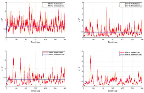
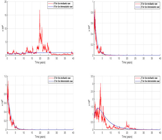
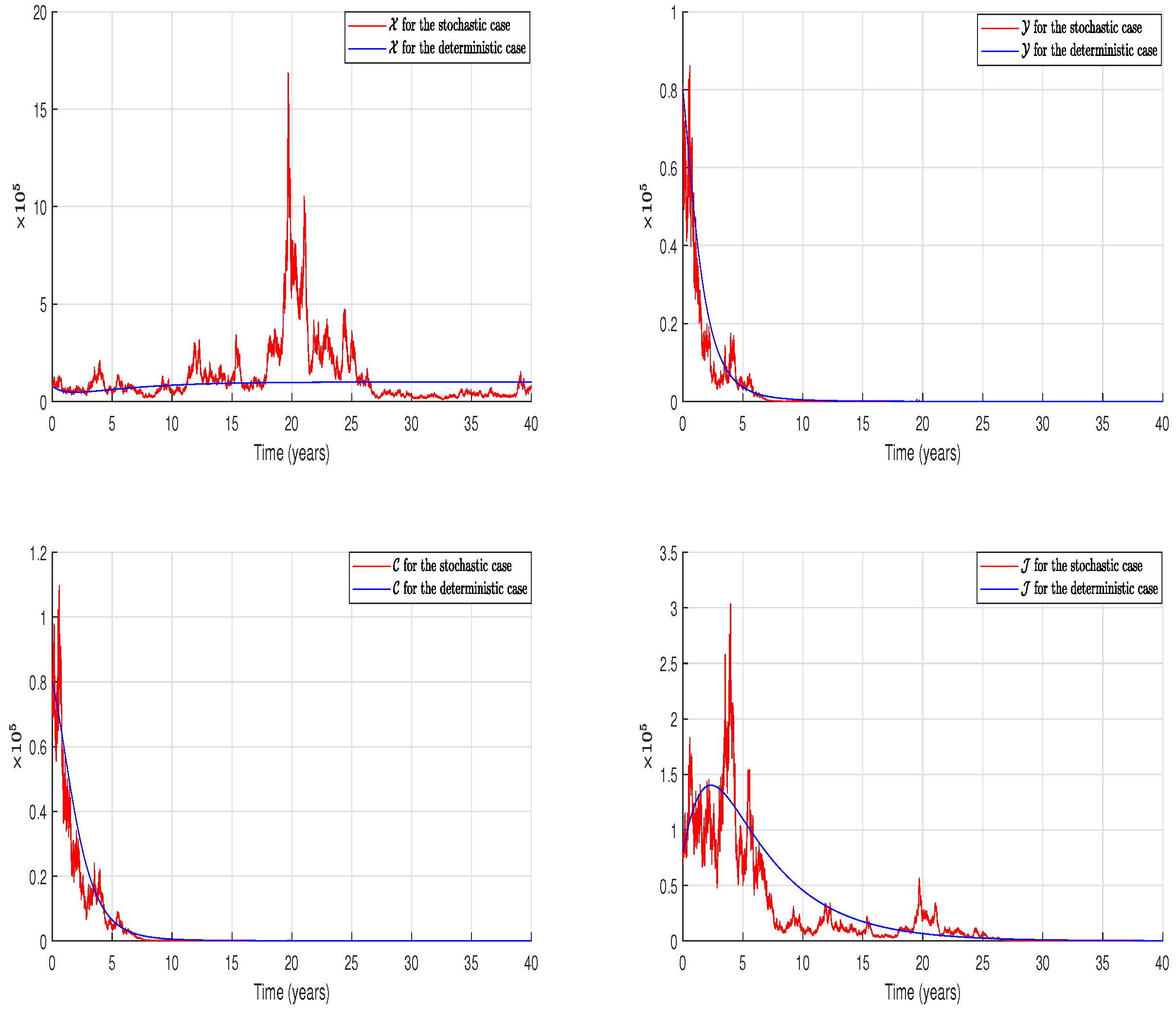
According to Theorem 4, poverty will be persistent, as shown in Figure 2.

Figure 2. Curves representing the solutions of the two models ((1) and (2)) for poverty persistence.

For the deterministic model (1), we have $\mathcal{R}=1.5556$. Figure 2 illustrates that the equilibrium state ${\mathsf{\Sigma }}_2=(0.802,0.7511,0.7409,1.668)$ exhibits locally asymptotic stability.

6.2. Empirical Test of the Statistical Stationarity

Adopting the same choice as that in the case of the poverty persistence, we deduce that the system (2) possesses a unique stationary probability measure according to Theorem 7. To exemplify this result, we perform four empirical tests.

6.2.1. Assessing Stationarity Using Histograms and Probability Density Functions

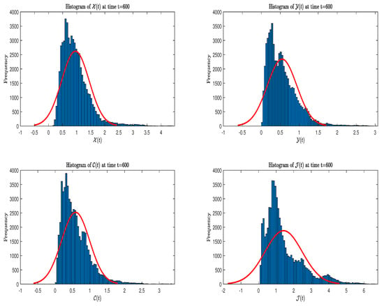
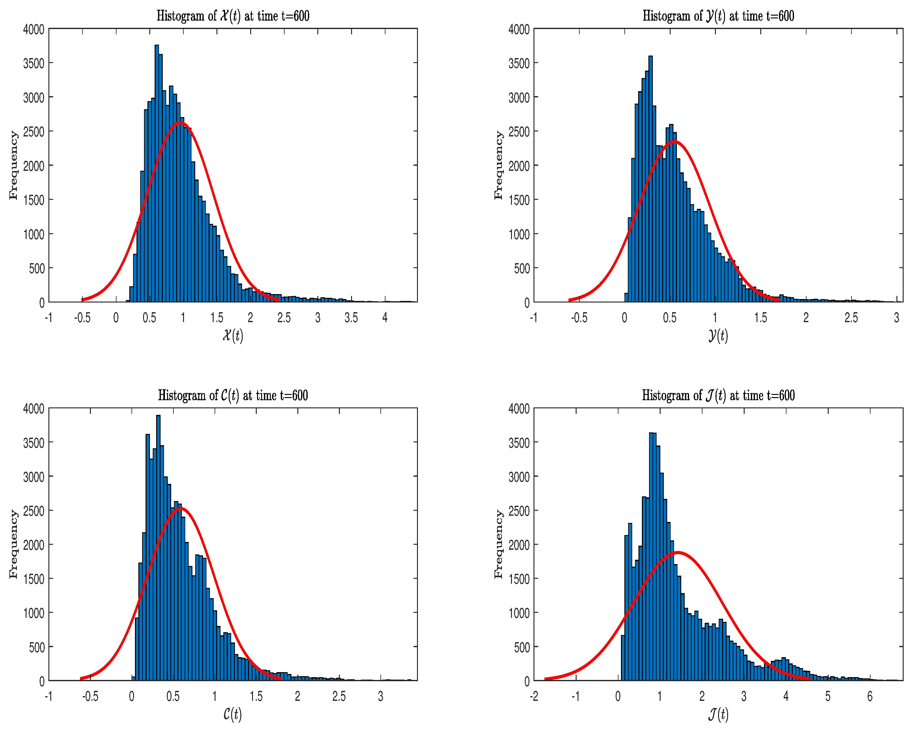
Figure 3 reveals the emergence of bell-shaped curves for the histograms and their density functions. This observation suggests that the realizations of the stochastic model (2) follow a Gaussian distribution, which is known to be stationary.

Figure 3. Histograms and their corresponding theoretical probability density functions for the stochastic model (2).

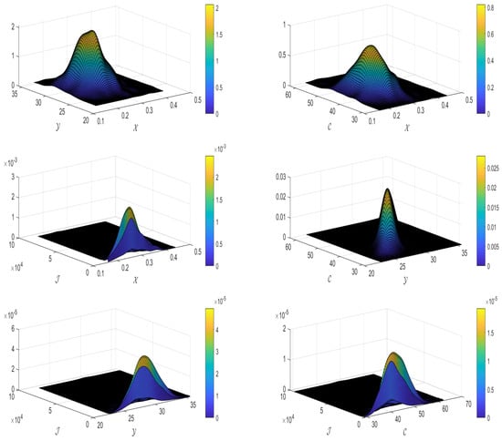
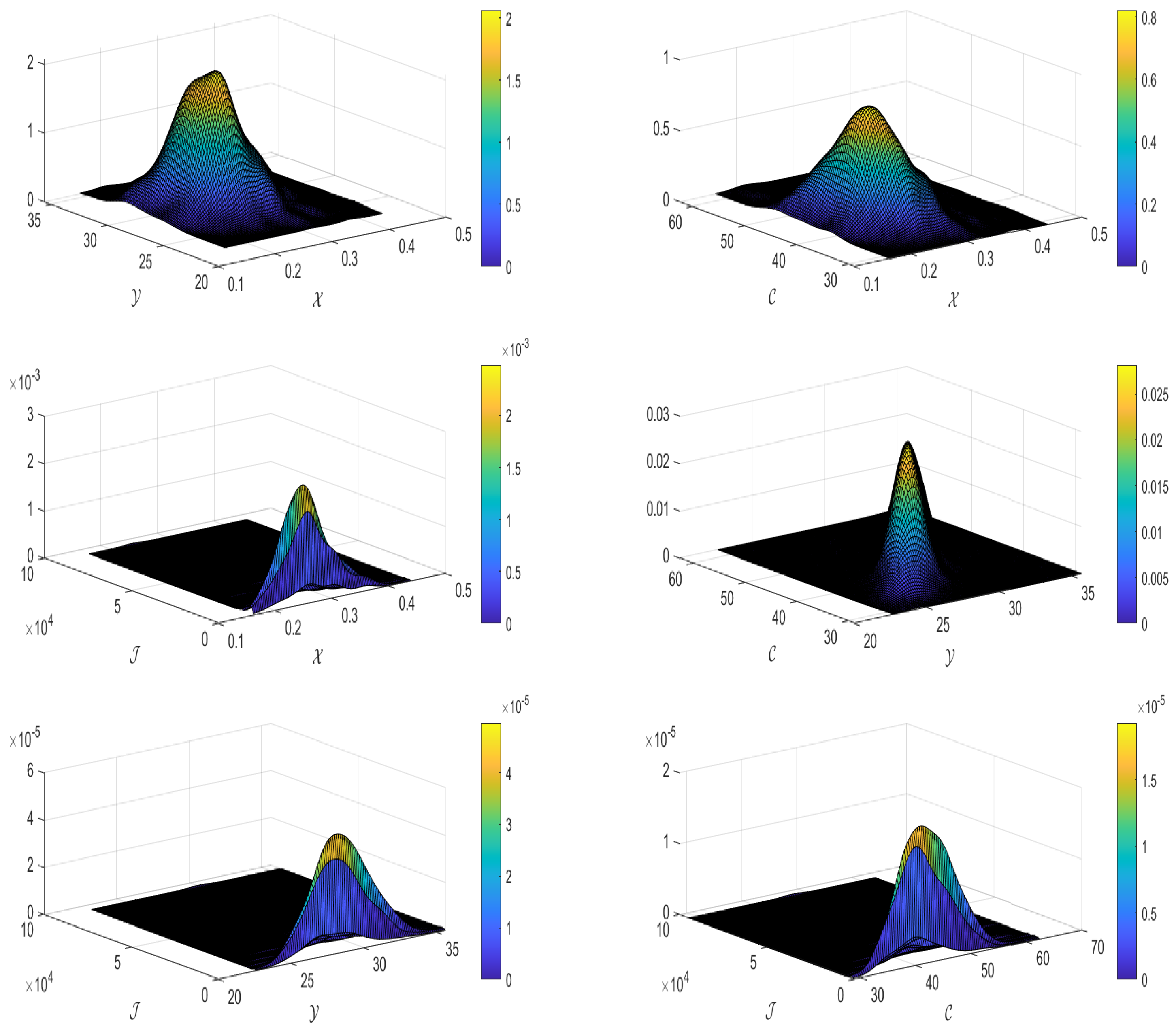
In the context of discussing the density function of a stochastic process, it is essential to revisit the concept of the joint density function of two stochastic processes. This concept proves to be valuable for characterizing the relationship between two potentially correlated or dependent stochastic processes. The bell-shaped form of the joint density function indicates that the two processes in question are distributed jointly according to a bivariate Gaussian distribution. To illustrate this statistical dependence within the stochastic model (2), we refer the readers to Figure 4, which substantiates that our model (2) possesses a stationary probability measure.

Figure 4. Three-dimensional visualization of the joint probability density functions related to the model (2).

6.2.2. Assessing Stationarity Through the Curves of the Mean and Variance

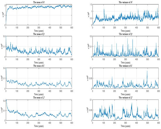
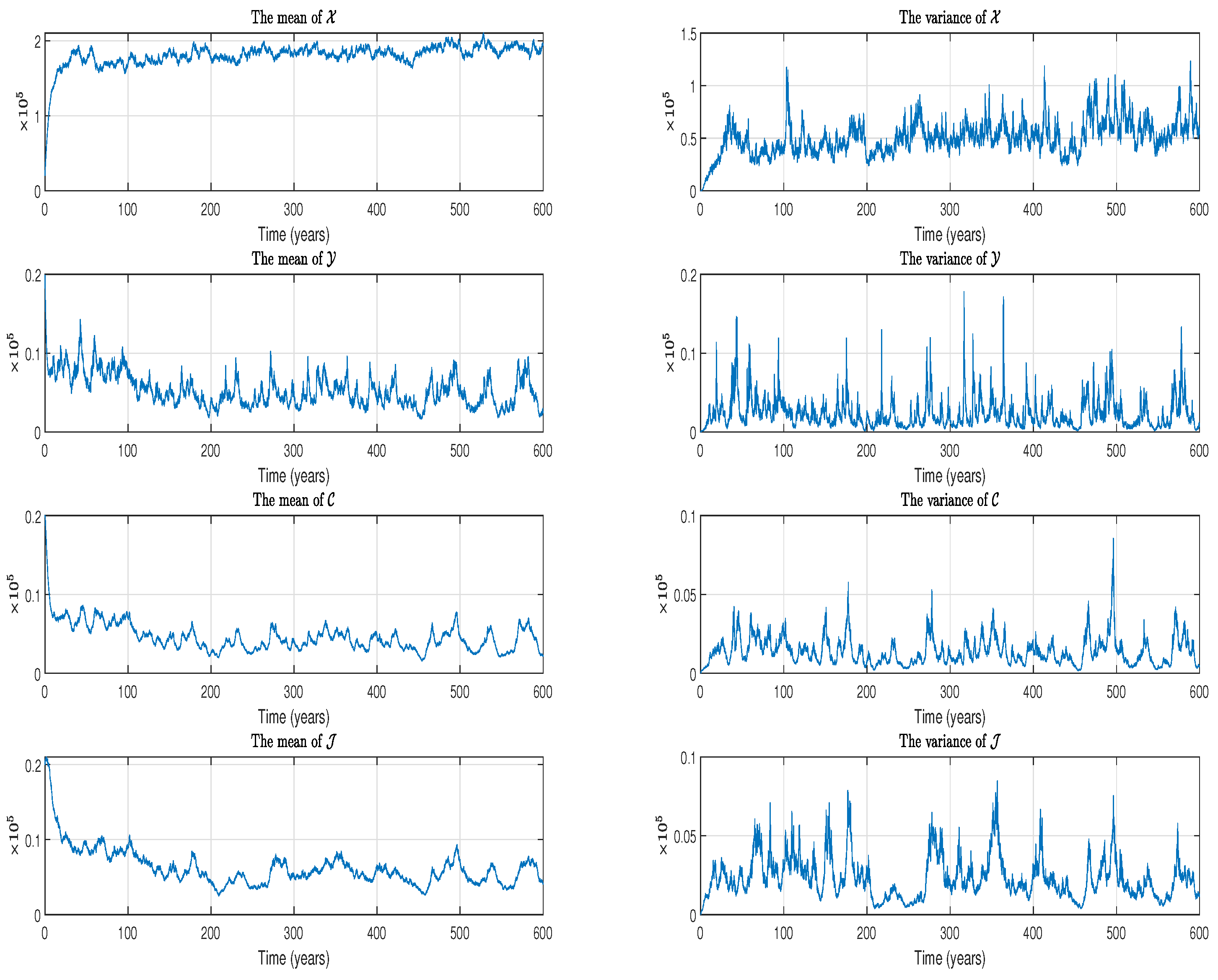
For a stochastic process adhering to a stationary distribution, the behaviors of the mean and variance exhibit distinct characteristics. Specifically, stationarity in the mean and variance implies that the expected value and variance of the stochastic process remain constant over time, resulting in their plots appearing as horizontal lines.

However, in the case of our stochastic model (2), which is stationary, the mean and variance display horizontal oscillations that do not exhibit significant variations. These fluctuations could be attributed to the diffusion term, the presence of periodic terms, or the nonlinear nature of the system (see Figure 5). Here, we can assert that the model exhibits weak stationarity without compromising its overall stationary properties.

Figure 5. Curves of the mean and the variance for the model (2). The blue curve depicts the mean (or variance) of the stochastic process (2) as a function of time, illustrating the expected value (or variability) of the process at each time point.

6.2.3. Assessing Stationarity Through Correlogram Analysis

The correlation function is an essential tool in statistics for analyzing the relationships between multiple variables or time points in a stochastic process. For a time series (${\mathsf{\Lambda }}_t$), the autocorrelation function, which measures the correlation between ${\mathsf{\Lambda }}_t$ and ${\mathsf{\Lambda }}_{t+h}$, is given by

$$\rho \left(h\right)={\displaystyle \frac{{\mathcal{R}}_{{\mathsf{\Lambda }}_t}\left(h\right)}{{\mathcal{R}}_{{\mathsf{\Lambda }}_t}\left(0\right)}},$$

where h is the time lag, and ${\mathcal{R}}_{{\mathsf{\Lambda }}_t}\left(h\right)=Cov\left({\mathsf{\Lambda }}_t,{\mathsf{\Lambda }}_{t+h}\right)$.

If the time series (${\mathsf{\Lambda }}_t$) is stationary, $Cov\left({\mathsf{\Lambda }}_t,{\mathsf{\Lambda }}_{t+h}\right)$ depends only on the lag (h) and is symmetric around $h=0$, i.e., ${\mathcal{R}}_{{\mathsf{\Lambda }}_t}\left(h\right)={\mathcal{R}}_{{\mathsf{\Lambda }}_t}(-h)$.

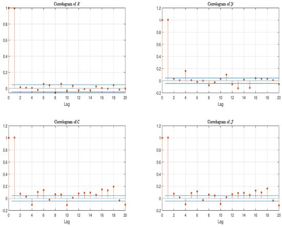
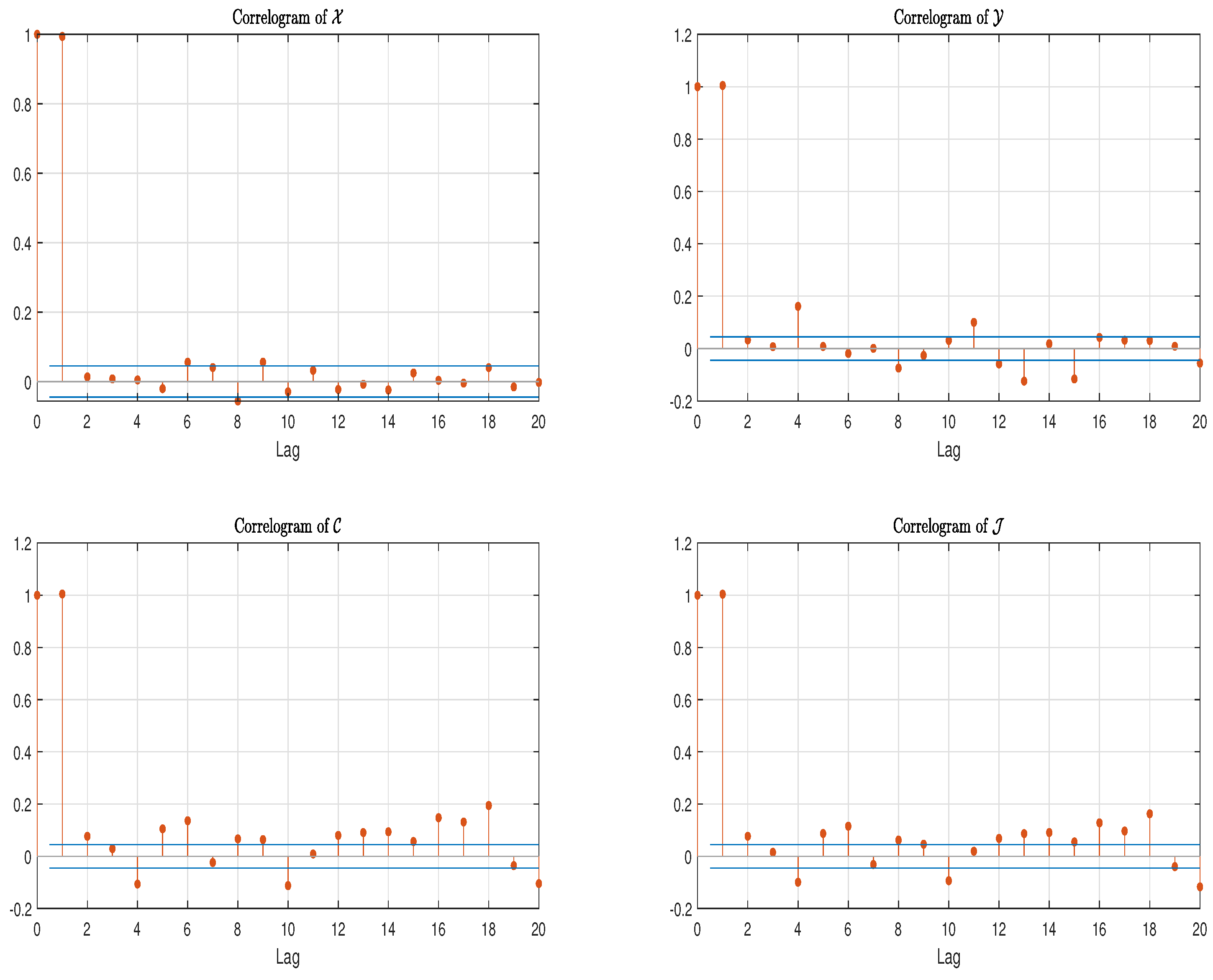
In the correlogram of ${\mathsf{\Lambda }}_t$, stationarity is indicated as follows: The autocorrelations should diminish rapidly as the lag (h) increases, without showing any ongoing trend. Moreover, there should not be any linear or exponential pattern in the decay of the autocorrelations.

Returning to the stochastic model (2), we observe that the aforementioned indications are fully validated in the correlograms of $\mathcal{X}$, $\mathcal{Y}$, $\mathcal{C}$, and $\mathcal{J}$, as illustrated in Figure 6.

Figure 6. Correlograms of the stochastic model (2). The two horizontal parallel blue lines represent the confidence intervals which help to identify which autocorrelations are statistically significant, while the red vertical lines indicate the lag positions.

6.2.4. Assessing Stationary Through Power Spectral Density

The Power Spectral Density (PSD) of a stochastic process is a function that specifies the distribution of the process’s variance over various frequencies. It is closely associated with the autocorrelation function and enables the analysis of the frequency characteristics of the stochastic process. Mathematically, the PSD of the stochastic process (${\mathsf{\Lambda }}_t$) presented previously is defined as the Fourier transform of the autocorrelation function ($\rho \left(h\right)$) as follows:

$$PSD\left({\mathsf{\Lambda }}_t\right)\left(\mathsf{{\rm Y}}\right)={\int }_{-\infty }^{\infty }\rho \left(h\right)e^{-2\pi \mathcal{I}h\mathsf{{\rm Y}}}dh,$$

where the notation $\mathcal{I}$ denotes the imaginary unit satisfying ${\mathcal{I}}^2=-1$, and $\mathsf{{\rm Y}}$ the frequency of ${\mathsf{\Lambda }}_t$.

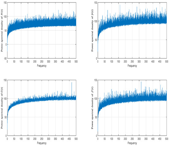
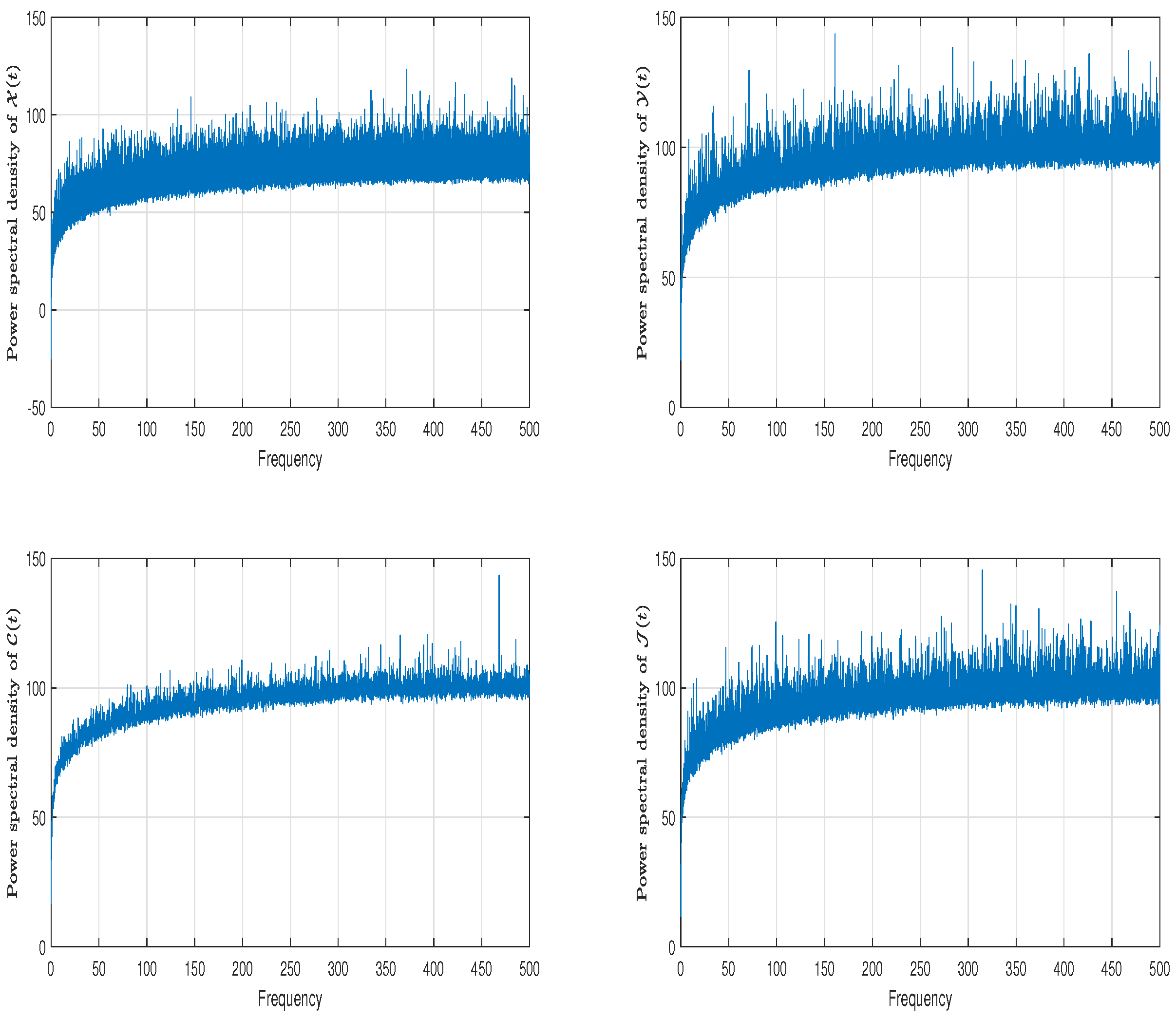
For a stationary process, the Power Spectral Density must be well defined and stable. This implies that the PSD plot should exhibit neither significant nor erratic variations with respect to the time or frequency. The PSD should be solely a function of the frequency, devoid of any explicitly time-dependent components.

If the PSD exhibits peaks at specific frequencies, this may suggest the presence of periodic or quasi-periodic elements within the process; however, these peaks do not inherently impact the stationarity of the process. The critical factor is that these peaks are frequency dependent and do not fluctuate with time.

Thus, Figure 7, depicting the Power Spectral Densities of the stochastic model (2), unambiguously demonstrates that the model is stationary.

Figure 7. Power spectral densities for the model (2). The blue curves in the figure represent the power spectral density of the solution to the model (2).

6.3. Empirical Test of Poverty Eradication

Let $\left(\mathcal{X}\right(0),\mathcal{Y}(0),\mathcal{C}(0),\mathcal{J}(0\left)\right)=(\mathrm{80,000},\mathrm{80,000},\mathrm{80,000},\mathrm{80,000}).$

$${\vartheta }_2=0.4352\mathrm{and}{\sigma }_1^2-\beta {\displaystyle \frac{\mu }{\mathcal{A}}}=-0.41.$$

By Theorem 5, poverty recedes exponentially with almost certainty, as shown in Figure 8. Moreover, this figure further indicates that the equilibrium ${\mathsf{\Sigma }}_1=(1,0,0,0)$ is stable because $\mathcal{R}=0.8182$.

Figure 8. Curves representing the solutions of the two models ((1) and (2)) for poverty eradication.

6.4. Empirical Test of the Stationarity and Ergodicity of the Total Population ($\psi$)

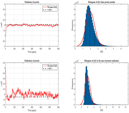
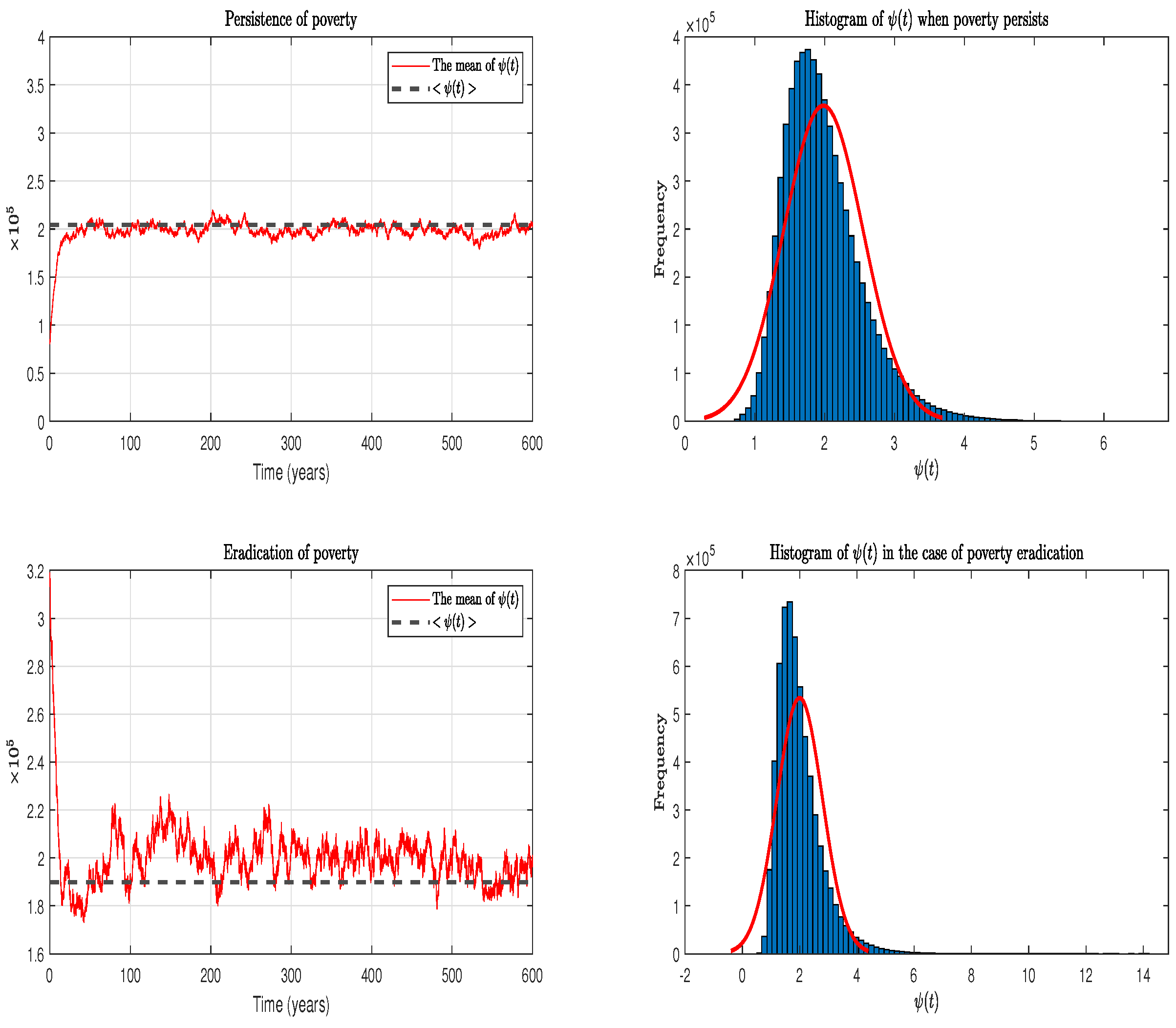
Theorem 2 asserts that the stochastic process ($\psi \left(t\right)$) remains stationary and ergodic in both poverty persistence and eradication scenarios. In previous tests, we have extensively discussed the concept of stationarity. Ergodicity pertains to the relationship where the statistical properties of a stochastic process over time are equivalent to the statistical properties observed across different samples or realizations. Formally, the process $\psi \left(t\right)$ is ergodic if ${\displaystyle {\displaystyle \underset{t⟶\infty }{lim}}}⟨\psi \left(t\right)⟩=\mathbb{E}\left(\psi \left(t\right)\right)$ almost surely, which is strongly supported by Figure 9.

Figure 9. Visual confirmation of the stationarity and ergodicity of $\psi \left(t\right)$ in both poverty persistence and eradication scenarios. The red line on the right of the figure is the curve of the two-dimensional density function of the process $\psi \left(t\right)$, corresponding to each histogram.

7. Conclusions

In summary, we have proposed and rigorously analyzed a model of poverty dynamics utilizing four stochastic differential equations. We began the study by confirming that the stochastic model (2) admits a single positive solution. Afterward, we showed that the system (2) admits a unique stationary probability measure if ${\vartheta }_1>1$ and ${\sigma }_2^2<{\displaystyle \frac{2}{3}}\mu$. This signifies that despite fluctuations, the long-term distribution of poverty levels within the population stabilizes. It also means that while individuals may move in and out of poverty, the proportion of the population in different poverty brackets reaches a steady state. This unique measure implies that there is only one such equilibrium distribution, and the system does not oscillate between different long-term patterns. Next, we revealed that volatility plays a critical role in shaping poverty dynamics. Specifically, the condition for poverty persistence (${\vartheta }_1>1$) highlights how increased uncertainty can entrench poverty. A higher ${\sigma }_1^2$, representing greater variance in the interdependence between susceptible and impoverished populations, signifies heightened economic instability, which, in turn, makes poverty more persistent. This could manifest as increased job insecurity, fluctuating incomes, or economic recessions, all of which hinder individuals’ ability to escape poverty. Similarly, a higher ${\sigma }_2^2$ value, reflecting greater variance in the death rate, can be interpreted as societal instability or the occurrence of health crises. These factors contribute to the persistence of poverty by disrupting social structures and economic productivity. Essentially, greater unpredictability in key economic and social factors exacerbates the challenge of overcoming poverty, even when average conditions might appear somewhat favorable. According to Theorems 4 and 7, we observe that the persistence of poverty implies that the model (2) admits a unique invariant measure. In other words, the overall statistical characteristics of poverty levels remain constant.

Conversely, the poverty eradication condition (${\vartheta }_2<1$) underscores the importance of stability for poverty reduction. The condition ${\sigma }_1^2\le \beta {\displaystyle \frac{\mu }{\mathcal{A}}}$ is particularly noteworthy, emphasizing that the variability in the interdependence (${\sigma }_1^2$) must be carefully controlled. If this variability exceeds a threshold determined by the average interdependence ($\beta$), the death rate ($\mu$), and the immigration rate of vulnerable individuals ($\mathcal{A}$) then poverty eradication becomes significantly more difficult, even if average conditions seem conducive to it. This finding suggests that policies aimed at mitigating economic volatility, promoting stable social safety nets, and ensuring consistent public health are crucial components of effective long-term poverty reduction strategies.

In our ongoing investigation of poverty dynamics, future research will broaden the scope of the stochasticity within the model (2). Specifically, we plan to introduce white noise to the remaining parameters to achieve a more comprehensive analysis of the uncertainty’s influence. A key consideration in this extension will be proving the non-divergence of the model’s solutions, ensuring its applicability for robust long-term analysis.

References

- Vakis, R.; Cafiero, C. Risk and Vulnerability Considerations in Poverty Analysis: Recent Advances and Future Directions. 2006. Available online: https://documents.worldbank.org/en/publication/documents-reports/documentdetail/414361468142164415/risk-and-vulnerability-considerations-in-poverty-analysis-recent-advances-and-future-directions (accessed on 24 June 2025).
- World Bank. Poverty: Overview. 2023. Available online: https://www.worldbank.org/en/topic/poverty/overview (accessed on 24 October 2023).
- Vemuri, V. Modeling of Complex Systems: An Introduction; Elsevier: Amsterdam, The Netherlands, 1978. [Google Scholar]
- Oduwole, H.K.; Shehu, S.L. A Mathematical Model on the Dynamics of Poverty and Prostitution in Nigeria. Math. Theory Model. 2013, 3, 74–79. [Google Scholar]
- Abdulwasaa, M.A.; Kawale, S.; Abdo, M.S.; Albalwi, M.D.; Shah, K.; Abdalla, B.; Abdeljawad, T. Statistical and computational analysis for corruption and poverty model using Caputo-type fractional differential equations. Heliyon 2024, 10, e25440. [Google Scholar] [CrossRef] [Scilit] [PubMed]
- Mushayabasa, S.; Bhunu, C.P.; Webb, C.R.; Dhlamini, M. A mathematical model for assessing the impact of poverty on yaws eradication. Appl. Math. Model. 2012, 36, 1653–1667. [Google Scholar] [CrossRef] [Scilit]
- Mitjà, O.; Marks, M.; Konan, D.J.P.; Ayelo, G.A.; González-Beiras, C.; Boua, B.; Houinei, W.; Kobara, Y.; Tabah, E.N.; Nsiire, A.; et al. Global epidemiology of yaws: A systematic review. Lancet Global Health 2015, 3, e324–e331. [Google Scholar] [CrossRef] [Scilit]
- Mitjà, O.; Hays, R.; Rinaldi, A.; Mcdermott, R.; Bassat, Q. New treatment schemes for yaws: The path toward eradication. Clin. Infect. Dis. 2012, 55, 406–412. [Google Scholar] [CrossRef] [Scilit] [PubMed]
- Becker, G.S. Crime and Punishment: An Economic Approach. J. Political Econ. 1968, 169–217. [Google Scholar] [CrossRef] [Scilit]
- Misra, A.K. Modeling the effect of police deterrence on the prevalence of crime in the society. Appl. Math. Comput. 2014, 237, 531–545. [Google Scholar] [CrossRef] [Scilit]
- Haiyun, Z.; Feng, Z.; Castillo-Chavez, C. The dynamics of poverty and crime. J. Shanghai Norm. Univ. 2014, 43, 486–495. [Google Scholar]
- Sachs, J.D. The End of Poverty: Economic Possibilities for Our Time; Penguin Publishing Group: London, UK, 2006. [Google Scholar]
- Stiglitz, J. Globalization and Its Discontents; Penguin Books Limited: London, UK, 2015. [Google Scholar]
- Sen, A. Poverty and Famines: An Essay on Entitlement and Deprivation; OUP Oxford: Oxford, UK, 1982. [Google Scholar]
- Banerjee, A.V.; Duflo, E. Poor Economics: A Radical Rethinking of the Way to Fight Global Poverty; PublicAffairs: New York, NY, USA, 2012. [Google Scholar]
- Palley, T.I. Plenty of Nothing: The Downsizing of the American Dream and the Case for Structural Keynesianism; Princeton University Press: Princeton, NJ, USA, 2000. [Google Scholar]
- Routh, E.J. A Treatise on the Stability of a Given State of Motion, Particularly Steady Motion: Being the Essay to Which the Adams Prize Was Adjudged in 1877, in the University of Cambridge; Macmillan and Company: New York, NY, USA, 1877. [Google Scholar]
- Gleick, J. Chaos: Making a New Science; Penguin Publishing Group: London, UK, 2008. [Google Scholar]
- Taleb, N.N. The Black Swan: The Impact of the Highly Improbable; Random House Publishing Group: New York, NY, USA, 2007. [Google Scholar]
- Mitchell, M. Complexity: A Guided Tour; Oxford University Press: Oxford, UK, 2009. [Google Scholar]
- Kelly, K. Out of Control: The New Biology of Machines, Social Systems, and the Economic World; Basic Books: New York, NY, USA, 2009. [Google Scholar]
- Yavuz, M.; Boulaasair, L.; Bouzahir, H.; Diop, M.A.; Benaid, B. The impact of two independent Gaussian white noises on the behavior of a stochastic epidemic model. J. Appl. Math. Comput. Mech. 2024, 23, 121–134. [Google Scholar] [CrossRef] [Scilit]
- Das, K.; Murthy, B.S.N.; Kabir, M.H.; Gani, M.O. A probabilistic model of competitive multi-ecological interactions for analyzing the impact of noise within sight of aquatic hyacinth. Decis. Anal. J. 2023, 7, 100231. [Google Scholar] [CrossRef] [Scilit]
- Boulaasair, L. Threshold properties of a stochastic epidemic model with a variable vaccination rate. Bull. Biomath. 2023, 1, 177–191. [Google Scholar] [CrossRef] [Scilit]
- Yuan, R.; Shi, Y.; Zhao, S.; Wang, W. The mKdV equation under the Gaussian white noise and Wiener process: Darboux transformation and stochastic soliton solutions. Chaos Solitons Fractals 2024, 181, 114709. [Google Scholar] [CrossRef] [Scilit]
- Boulaasair, L.; Bouzahir, H.; Vargas, A.N.; Diop, M.A. Existence and uniqueness of solutions for a stochastic urban-population growth model. Front. Appl. Math. Stat. 2022, 8, 960399. [Google Scholar] [CrossRef] [Scilit]
- Zeng, Y.; Zhang, Y.; Huang, N. A stochastic fractional differential variational inequality with Lévy jump and its application. Chaos Solitons Fractals 2024, 178, 114372. [Google Scholar] [CrossRef] [Scilit]
- Mood, A.M.F.; Graybill, F.A.; Boes, D.C. Introduction to the Theory of Statistics; McGraw-Hill: New York, NY, USA, 1974. [Google Scholar]
- Mao, X. Stochastic Differential Equations and Applications; Elsevier Science: Amsterdam, The Netherlands, 2007. [Google Scholar]
- Liptser, R.S. A strong law of large numbers for local martingales. Stochastics 1980, 3, 217–228. [Google Scholar] [CrossRef] [Scilit]
- Gallager, R.G. Stochastic Processes: Theory for Applications; Cambridge University Press: Cambridge, UK, 2013. [Google Scholar]
- Taylor, H.M.; Karlin, S. An Introduction to Stochastic Modeling; Elsevier Science: Amsterdam, The Netherlands, 2014. [Google Scholar]
- Allen, L.J.S. An Introduction to Stochastic Processes with Applications to Biology; CRC Press: Boca Raton, FL, USA, 2010. [Google Scholar]
- Bressloff, P.C. Stochastic Processes in Cell Biology; Springer: Berlin/Heidelberg, Germany, 2014. [Google Scholar]
- Lande, R.; Engen, S.; Saether, B.E. Stochastic Population Dynamics in Ecology and Conservation; Oxford University Press: Oxford, UK, 2003. [Google Scholar]
- Ross, S.M. Introduction to Probability Models; Academic Press: New York, NY, USA, 2004. [Google Scholar]
- Khasminskii, R. Stochastic Stability of Differential Equations; Springer: Berlin/Heidelberg, Germany, 2012. [Google Scholar]
- Kiouach, D.; Boulaasair, L. Stationary distribution and dynamic behaviour of a stochastic SIVR epidemic model with imperfect vaccine. J. Appl. Math. 2018, 2018, 1291402. [Google Scholar] [CrossRef] [Scilit]
- Han, B.; Jiang, D. Stationary distribution and extinction of a hybrid stochastic vegetation model with Markov switching. Appl. Math. Lett. 2023, 139, 108549. [Google Scholar] [CrossRef] [Scilit]
- Mdaghri, A.; Lakhal, M.; Taki, R.; Fatini, M.E. Ergodicity and stationary distribution of a stochastic SIRI epidemic model with logistic birth and saturated incidence rate. J. Anal. 2024, 32, 3249–3276. [Google Scholar] [CrossRef] [Scilit]
- Da Prato, G.; Zabczyk, J. Ergodicity for Infinite Dimensional Systems; Cambridge University Press: Cambridge, UK, 1996. [Google Scholar]
- Bhattacharya, R.; Waymire, E. Stochastic Processes with Application; John Wiley & Sons: New York, NY, USA, 1990. [Google Scholar]
- Zhou, B.; Jiang, D.; Han, B.; Hayat, T. Threshold dynamics and density function of a stochastic epidemic model with media coverage and mean-reverting Ornstein–Uhlenbeck process. Math. Comput. Simul. 2022, 196, 15–44. [Google Scholar] [CrossRef] [Scilit]
- Tong, J.; Zhang, Z.; Bao, J. The stationary distribution of the facultative population model with a degenerate noise. Stat. Probab. Lett. 2013, 83, 655–664. [Google Scholar] [CrossRef] [Scilit]
- Higham, D.J. An algorithmic introduction to numerical simulation of stochastic differential equations. SIAM Rev. 2001, 43, 525–546. [Google Scholar] [CrossRef] [Scilit]
Disclaimer/Publisher’s Note: The statements, opinions and data contained in all publications are solely those of the individual author(s) and contributor(s) and not of MDPI and/or the editor(s). MDPI and/or the editor(s) disclaim responsibility for any injury to people or property resulting from any ideas, methods, instructions or products referred to in the content. |
© 2025 by the authors. Licensee MDPI, Basel, Switzerland. This article is an open access article distributed under the terms and conditions of the Creative Commons Attribution (CC BY) license (https://creativecommons.org/licenses/by/4.0/).