Abstract
The morphology of blood vessels in retinal fundus images is a key biomarker for diagnosing conditions such as glaucoma, hypertension, and diabetic retinopathy. This study introduces a deep learning-based method for automatic blood vessel segmentation, trained from scratch on 44 clinician-annotated images. The proposed architecture integrates Bidirectional Long Short-Term Memory (Bi-LSTM) layers with dropout to mitigate overfitting. A distinguishing feature of this approach is the column-wise processing, which improves feature extraction and segmentation accuracy. Additionally, a custom data augmentation technique tailored for retinal images is implemented to improve training performance. The results are presented in their raw form—without post-processing—to objectively assess the method’s effectiveness and limitations. Further refinements, including pre- and post-processing and the use of image rotations to combine multiple segmentation outputs, could significantly boost performance. Overall, this work offers a novel and effective approach to the still unresolved task of retinal vessel segmentation, contributing to more reliable automated analysis in ophthalmic diagnostics.
Keywords:
retinal blood vessel segmentation; bi-directional LSTM (Bi-LSTM); medical image analysis; deep learning MSC:
68T45
1. Introduction
The human retina offers a unique window into systemic health, where subtle microvascular changes—arteriolar narrowing, venular widening, increased tortuosity—signal early warning signs of hypertension, diabetes, and cardiovascular disease [1]. These biomarkers can be detected years before clinical symptoms [2] and are quantified by segmentation of the retinal vessels. However, despite this diagnostic potential, automated segmentation remains an unsolved challenge: errors propagate into critical biomarkers such as the arteriole-to-venule ratio (AVR), a known predictor of stroke risk [3], and they actively undermine clinician and patient trust in AI systems [4].
Current approaches, dominated by convolutional neural networks (CNNs) and vision transformers (ViTs), achieve impressive precision on curated benchmarks such as DRIVE and STARE [5]. In the real world, however, baseline U-Net–style models under-segment faint capillaries, often missing entire small vessels [6,7]; hallucinate vessel-like artifacts near pathological lesions [8]; and suffer catastrophic performance drops in unseen devices or demographics [9]. Mounting evidence traces these failures to a fundamental mismatch between the need for global vascular continuity [10] and the inherently local, grid-based processing of standard CNN/transformer architectures [11].
Competing explanations. One line of work claims that annotation noise and domain shift, rather than model design, are the real bottlenecks: when masks are cleaned and multidevice data are used, standard CNNs already have near-perfect scores [9,12]. A second view blames local receptive field of convolutions and pushes for global context solutions: self-attention transformers or explicit connectivity losses. A recent transformer model reports markedly improved vessel connectivity on DRIVE, STARE and CHASE_DB1 [13], while connectivity-aware losses also close gaps [11]. Our sequence-first Bi-LSTM offers an orthogonal test of these competing hypotheses.
1.1. The Data Efficiency Dilemma
Deep CNNs are notoriously data-hungry, with large reviews noting the need for thousands of pixel-accurate masks [14], yet the largest vessel datasets still top out at 500–800 expert-annotated images [15,16]. However, interobserver variability exceeds 20% for capillaries [9,17], introducing noise into the training. Although synthetic data and augmentation mitigate this, they risk distorting vascular morphology or hiding failures behind post-processing. Common low-level transforms—JPEG compression, aggressive rotation or scaling—can bias vessel caliber and fractal metrics [18] and may erase capillaries unless augmentation is vessel aware [19]; comprehensive reviews echo these pitfalls across medical modalities [20]. A paradigm shift is needed: methods that learn structural priors (e.g., vessel connectivity) from limited data while preserving interpretability [21].
1.2. Sequential Reasoning with Bi-LSTMs
Bidirectional Long Short-Term Memory (Bi-LSTM) networks, originally devised for sequential signals such as language and speech, offer an unconventional solution for fundus analysis. Recent work by Marti-Puig et al. demonstrated that a column-wise Bi-LSTM can extract continuous shorelines from time-lapse coastal imagery with high fidelity [22]. Motivated by that success, we treat each retinal image column as a 1-D sequence so that a Bi-LSTM can propagate evidence bidirectionally, enforcing the global vascular continuity that patch-based CNNs often overlook [11]. Earlier hybrids, most notably BCDU-Net [23], grafted Bi-LSTM blocks onto a U-Net backbone but still inherited convolutional biases. In the present work, we eliminate convolutions entirely: raw columnar sequences are processed by a pure Bi-LSTM backbone, forcing the network to infer retinal topology from sequential context—a structural prior that aligns naturally with vascular anatomy.
1.3. Transparency Through Minimalism
Our approach prioritizes simplicity and interpretability.
- Data efficiency: Processing each 1024-pixel column as an independent sequence inflates the 44 training images (drawn from the 54 publicly released RETA-IDRiD images) into 45,056 sequences, reducing annotation demands.
- Rotation ensembles: A single right-angle rotation (0°, 90°, 180°, 270°) is always applied. For data-limited experiments, we also used eleven off-axis rotations (15°–315°, see Section 2.6), which yielded 540,672 sequences. These angles preserve vessel morphology better than arbitrary elastic warps.
- Raw outputs: Publicly released probability maps expose errors (e.g., optical disc glare, hemorrhages), fostering trust and guiding clinical refinements.
1.4. Contributions and Implications
This work demonstrates the following:
- In our internal test fold of ten images (18% of the accessible data), the best Bi-LSTM attains 95.6% pixel accuracy and an MCC of 0.70 (see Tables 5 and 7). All results are reported before any morphological post-processing. These first-cut results do not yet surpass strong CNN/ViT baselines on the official 27-image RETA leader board, but they show that pure sequence-first reasoning can reach parity on fully public data, warranting hybrid architectures in future work.
- Data-efficient training through sequential processing, sidestepping the need for massive annotated datasets.
- Failure-aware transparency, critical for clinical adoption, by exposing edge cases like tortuous vessels.
Although not yet surpassing state-of-the-art CNNs, our results validate sequence-first reasoning as a complementary paradigm. Future work could integrate Bi-LSTMs with CNNs in hybrid architectures, combining local texture analysis with global continuity modeling, a promising direction for robust, interpretable diagnostic tools.
From this point forward, the article is organized as follows. Section 2 details the RETA-IDRiD dataset, the 44/10 data split, CIE–Lab color space conversion, and rotation-based data augmentation and describes the full column-wise processing pipeline, including three Bi-LSTM variants and the exact MATLAB 2024b training protocol. Section 3 presents pixel-level performance metrics for all models on the held-out RETA fold, accompanied by raw (pre-morphology) confusion matrices and color-coded overlays for true positives, false positives, and false negatives. Section 4 discusses common failure modes of the model, such as missed capillaries, lesion-induced hallucinations, and glare artifacts, relating these issues to architectural design choices and domain-shift vulnerabilities. Finally, Section 5 summarizes the key findings.
2. Materials and Methods
2.1. Datasets
Primary data. All experiments use the RETA–IDRiD vascular tree subset, released with the RETA benchmark, [12,24]. It contains 81 color fundus images (45° field of view (FOV), 4288 × 2848 px, saved as 1024 × 1024 crops in our pipeline) with dense annotations for vessels, artery/vein identity, bifurcations, and skeletons. We follow the official split: 54 images for training/validation and 27 for hold-out testing. IDRiD images are deidentified and publicly licensed for research; no additional ethical approval is required.
Of the 54 RETA-IDRiD images labeled, 27 are reserved by the organizers as a challenge test set—the masks are not publicly released and evaluation is possible only by blind submission to the leaderboard. To keep our study fully reproducible, we therefore work solely with the 54 accessible images. Ten (18%) are left as an internal test fold, stratified to match the prevalence of lesions in the entire set (two heavily diseased eyes, eight mild/normal). The remaining 44 form the training pool. This 80/20 split is standard practice for small medical datasets and avoids data leakage while preserving enough samples for model fitting and augmentation.
Why RETA? Compared with legacy sets such as DRIVE [25], STARE [26] or CHASE_DB1 [27], RETA offers (i) cleaner masks (semi-automated, adjudicated), (ii) lesion variability (exudates, hemorrhages) that stresses false positive control, and (iii) structural labels enabling future benchmarks at the artery/vein or tree level. For video-based generalization, we point the reader to the recent RVD dataset, [28], left for future work.
2.2. Pre-Processing
Each image is center-cropped to the 1024 × 1024 field supplied by RETA and converted to CIE–Lab. A simple circular mask excludes the black background. No color normalization is applied—deliberately—to expose any domain-shift brittleness.
2.3. Image Processing Strategy: Column-Based Approach
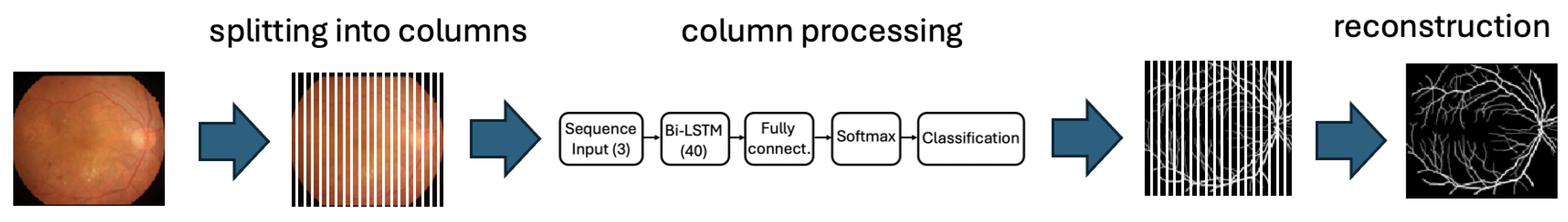
As mentioned above, the distinctive aspect of our segmentation approach lies in the processing of retinal images column by column. This involves dividing each image into column vectors and, for each of these vectors, using a neural network to determine which pixels correspond to the retinal background and which correspond to blood vessels. In our case, the images have a resolution of 1024 × 1024 pixels, meaning that we process 1024 columns per image. These columns are subsequently reassembled in the correct order to reconstruct the segmentation of the original image.
Deep learning-based networks require large amounts of data for effective training, and the annotation process is time consuming and must be carried out by domain experts. The annotated dataset available for training is therefore limited. By changing the training unit from full images to individual image columns, we effectively increase the number of training samples by a factor of 1024. This significantly expands the annotated dataset and provides sufficient data to train deep learning models.
A key step in our approach is interpreting each column as a time series and processing it using neural networks based on LSTM layers, which are particularly well suited for handling sequential data.
The image processing workflow is illustrated in Figure 1, which shows how the image is decomposed into individual columns, how an estimate is obtained for each column, and how the final vessel-background segmentation is reconstructed by combining the estimations from all columns.
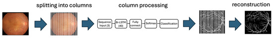
Figure 1.
The image processing workflow highlights the key steps: starting with the separation of the image into columns, followed by the individual processing of each column through the neural network, and finally the reconstruction of the column-wise results to obtain the desired segmentation.
2.4. Long Short-Term Memory (LSTM) Networks
LSTM networks operate based on two core state vectors. The first, the hidden state vector , represents both the internal state and the output of the LSTM layer at time step t. The second, the cell state vector , is designed to preserve longer-term dependencies across the sequence. At each time step, the network selectively updates by adding or removing information through gated mechanisms.
An LSTM cell typically consists of four gates: (1) the input gate, denoted by the vector , which controls how much new information is incorporated into the cell state; (2) the forget gate, , which modulates the removal of past information from the cell state ; (3) the cell candidate gate, , which provides new candidate values to be added to the state; and (4) the output gate, , which determines the extent of information to be passed to the hidden state. These gates operate in conjunction to maintain and update the internal memory of the LSTM.
Figure 2a illustrates the internal architecture of an LSTM cell and the gate outputs at time t, from left to right: , , , and . The figure also displays the input vector and the computations that update both and using their respective values and from the previous time step ().
Figure 2.
(a) The LSTM cell. (b) The information flow in a bidirectional LSTM (Bi-LSTM) layer.
The LSTM network has three types of parameters: input weights in matrix , the recurrent weights in , and biases in the vector . The matrix combines information from the input , while controls the contribution of the previous hidden state , while adds a bias. Each of these parameters is partitioned into subcomponents corresponding to the four gates:
Each gate computes its output based on the current input and the hidden state from the previous time step according to the following:
Notice, for instance, the input gate vector is calculated as the weighted input plus the recurrent contribution and the bias . The activation function , a logistic sigmoid defined as , is applied element-wise to the resulting vector. The remaining gate vectors are computed analogously with the particularity that in Equation (4), the activation function is the hyperbolic tangent, , which also is applied element-wise.
The gate outputs obtained in Equations (2)–(5) with the cell state are used to update the cell and hidden vector states and as follows:
where ⊙ denotes the Hadamard (element-wise) product. Notice that the cell state is updated by selectively retaining prior information () and incorporating new candidate content (). The hidden state , which serves as the LSTM output at time t, is derived from the cell state in the form pondered by the output gate vector .
As mentioned, the LSTM network processes image columns, where each column is represented as a sequence of vectors of size 1 × 3 over 1024 time steps. Each vector , with t ranging from 1 to 1024 (since the input images are of size 1024 × 1024), contains the features corresponding to the pixel at position t in the image column, expressed in the CIE–Lab color space. Consequently, all input sequences have a fixed length of 1024, and each input vector encodes the color information of a single pixel in that column. The LSTM network produces a binary output vector of dimensions 1024 × 1, with each entry indicating whether the corresponding input pixel is classified as vessel or background. The initial hidden and cell states, denoted by and , define the starting conditions of the network and can be initialized as zero vectors.
In the LSTM networks, the information is processed sequentially along the column. At each step t, the network leverages the information accumulated from previous steps, capturing both short-term and long-term dependencies in the sequence. As the input sequence consists of the complete set of pixels in an image column, and there is no temporal constraint on data availability, we propose using a bidirectional LSTM (Bi-LSTM) structure, which enables the model to learn dependencies in both directions along the sequence, thus improving its capacity to model contextual relationships across the entire column. The output of the Bi-LSTM is computed by combining the outputs of the two LSTM layers from an expression of the following type:
where are the outputs of the LSTM cell that processes the column in the forward direction and are the outputs of the LSTM cell that processes the image column in the backward direction. The symbol stands for the activation function. The matrices and contain the weights used to combine the outputs of the forward and backward cells in the Bi-LSTM layer and the biases. Figure 2b provides a graphical representation of the information flow within a bidirectional LSTM (Bi-LSTM) layer.
2.5. Network Architectures
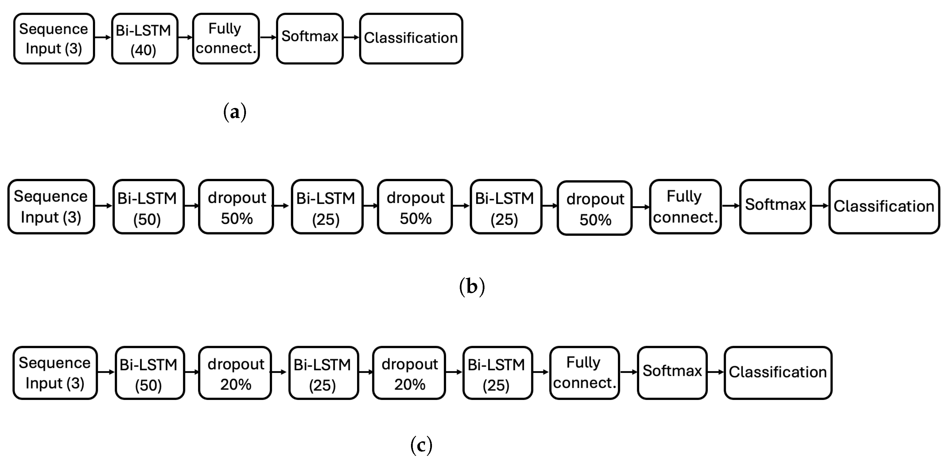
Figure 3 presents the three Bi-LSTM architectures explored in this study, each corresponding to a distinct experiment designed to explore the impact of depth and regularization.
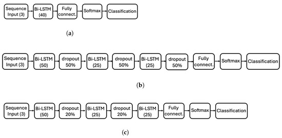
Figure 3.
Diagram of the three ANN architectures evaluated in this study. (a) Simple architecture with a single Bi-LSTM layer (40 hidden units). (b) Deeper architecture with three Bi-LSTM layers (50-25-25 hidden units) and 50% dropout between layers. (c) Modified deep architecture with the same Bi-LSTM layers as (b), but with reduced dropout (20%) between the first two layers and no dropout after the third layer. Each architecture corresponds to a different experiment.
- Architecture 1 (Figure 3a): A simple configuration consisting of a single Bi-LSTM layer with 40 hidden units, serving as our baseline to test whether minimalist column-wise processing can achieve satisfactory performance (14.2 K learnable parameters).
- Architecture 2 (Figure 3b): A deeper configuration with three Bi-LSTM layers (50-25-25 hidden units) interleaved with 50% dropout layers to improve robustness and prevent overfitting (62.7 K learnable parameters).
- Architecture 3 (Figure 3c): Similar to Architecture 2 but with reduced dropout (20%) between the first two layers and no dropout after the third layer, exploring the effect of relaxed regularization constraints (62.7 K learnable parameters).
For baseline comparisons, we also implement the following.
- U-Net: Standard U-Net architecture with 61 layers processing full 1024 × 1024 fundus images, totaling 31M parameters.
- DeepLab v3+: A ResNet-18 based DeepLab v3+ with 99 layers and 20.6 M learnable parameters.
- ViT-Tiny: We adopt the standard vit_tiny_patch16_224 encoder (12 transformer blocks, hidden size 192, three attention heads per block) with 5.72 M trainable parameters as originally reported by Touvron et al. [29] and subsequently summarized in the lightweight-ViT survey of Wang et al. [30].
2.6. Data Augmentation, Training and Hyperparameter Selection
To train and evaluate the models, the dataset is divided into two subsets: one for model training and one for testing. In all experiments, the first 44 images were used for training, while the remaining 10 were used for testing. This deterministic split allows for a consistent comparison across experiments and different architectures by ensuring that all models are trained and evaluated on exactly the same data. This avoids the variability that could be introduced by random partitioning, which might otherwise affect model training and test results.
2.6.1. Bi-LSTM Training
The network was trained using the ADAM optimizer with a gradient decay factor of 0.9 and a squared gradient decay factor of 0.999. The initial learning rate was set to and remained constant throughout training, as no learning rate schedule was applied. Training was performed for a maximum of 8 epochs with a mini-batch size of 2048, and data was shuffled once at the beginning of training. The L2 regularization coefficient was set to to mitigate overfitting, and gradient clipping was applied using the L2 norm method with a threshold of 1. The training was executed on a CPU environment.
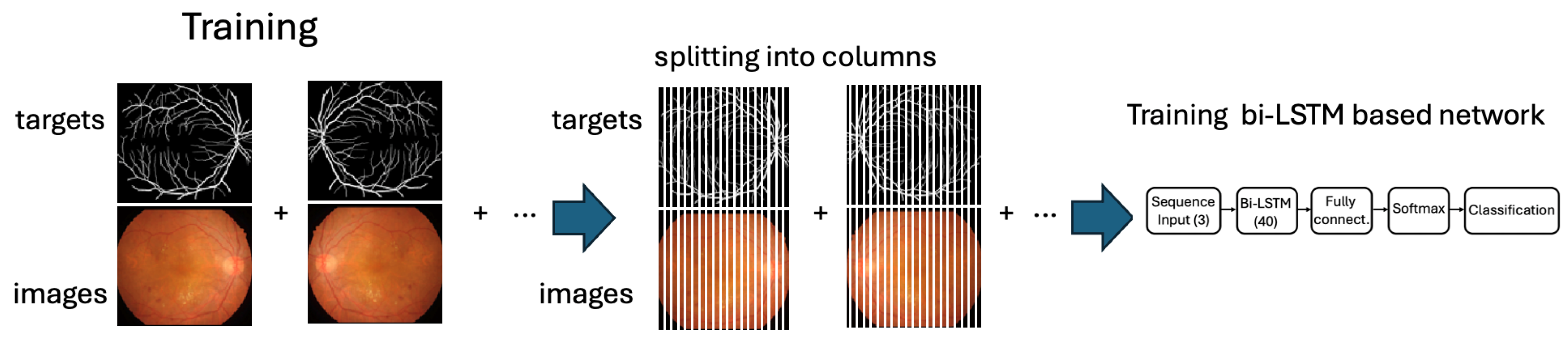
Figure 4 depicts the training workflow of the proposed approach, which relies on column-based image processing. So, once the model is trained, it is applied to the test set. The testing procedure consists of processing the labeled images reserved for testing, as described in Figure 1, and comparing the results provided by the network with the corresponding target values by performing a quantitative evaluation and also a qualitative assessment for interpreting the results and validating the model’s performance.
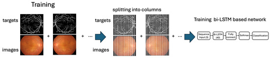
Figure 4.
The training workflow highlights the separation of the image and targets into columns that are processed as time-series sequences.
2.6.2. U-Net Training
The U-Net model was trained using the ADAM optimizer. The initial learning rate was set to , and no learning rate scheduling was applied. The optimizer’s hyperparameters included a gradient decay factor of 0.9 and a squared gradient decay factor of 0.999, with a small epsilon value () to ensure numerical stability. L2 regularization was applied with a weight of to reduce overfitting. Training was performed over a maximum of 50 epochs with a mini-batch size of 4. The training data was shuffled at the beginning of each epoch. The training was executed on a CPU environment.
2.6.3. DeepLab v3+ Training
The network was trained using the Stochastic Gradient Descent with Momentum (SGDM) optimizer. The training configuration included a momentum of 0.9 and an initial learning rate of 0.001, with a total of 60 epochs. Mini-batches of size 8 were used, and the data were shuffled at every epoch. L2 regularization was set to to prevent overfitting. The training was executed on a CPU environment.
2.6.4. Vision Transformer Training
All hyperparameters reflect recurrent experiments: class-weighted cross-entropy, ADAMW (, weight decay ) and the deterministic 44/10 RETA–IDRiD split. A single epoch sweeps ≈0.5 M patches—∼12× more gradient steps than one full-image epoch of the Bi-LSTM. During inference, softmax probabilities are stitched back to a single mask and thresholded at 0.5, exactly as for the Bi-LSTM pipeline.
So, each image in the training group and each corresponding target is decomposed into columns, and all the vectors obtained from the set of training and all the corresponding target vectors are aggregated and used to train the model. This operation yields 44 × 1024 = 45,056 labelled instances.
As a data augmentation strategy, given the circular shape of the retinas centered within square images, the most natural approach is to apply image rotations. By simply rotating the images by 90°, 180°, and 270°, the number of labeled instances can be increased by a factor of four without the need for additional image processing. This augmentation helps reduce overfitting by exposing the model to different orientations of the same anatomical structures, which improves its ability to generalize to unseen data. If further (non-right-angle) rotations are introduced, minimal additional processing of both the images and their corresponding target masks will be required to preserve alignment. However, in all the experiments, the data augmentation strategy consisted of applying the same set of rotations, specifically at angles , , , , , , , , , , and . As a result, a total of labeled instances were generated.
2.7. Performance Evaluation
In the present case, we compare the pixel classification results of each reconstructed image after being processed column by column with its corresponding target. To evaluate binary classification performance, the confusion matrix, a 2 × 2 contingency table, is used. In this matrix, pixels that are correctly classified as positive are referred to as true positives (TPs), while negative pixels incorrectly classified as positive are called false positives (FPs). Similarly, pixels that are correctly classified as negative are termed true negatives (TNs), and positive pixels misclassified as negative are known as false negatives (FNs). In addition to evaluating the results using TPs, TNs, FPs, and FNs, we use these values to compute the following performance metrics.
These metrics provide a comprehensive evaluation of binary classification performance, especially in contexts where class imbalance may affect simple accuracy-based assessments. While accuracy gives an overall sense of correctness, it may be misleading when one class dominates. In such cases, recall and specificity become particularly important, as they reflect the model’s ability to correctly identify positive and negative instances, respectively.
Precision complements recall by indicating the reliability of positive predictions, which is essential in applications where false positives carry a significant cost. The F1-score, as the harmonic mean of precision and recall, offers a single metric that balances both aspects and is especially useful when the dataset has an uneven class distribution.
The false-positive rate (FPR) highlights the proportion of negative cases incorrectly labeled as positive and is a key component in Receiver Operating Characteristic (ROC) analysis. Finally, the Matthews Correlation Coefficient (MCC) provides a robust evaluation that considers all four components of the confusion matrix (TPs, TNs, FPs, FNs), making it a particularly valuable metric for assessing model performance on imbalanced datasets.
3. Results
This section is organized as follows. Section 3.1 provides an in-depth ablation of our primary contribution, the proposed Bi-LSTM model. Section 3.2, Section 3.3 and Section 3.4 present results from three state-of-the-art baselines, a U-Net, a DeepLab v3+ (both full-image CNNs), and a parameter-matched Vision Transformer (ViT-Tiny), for direct comparison against our approach. We conclude with a comprehensive summary table (Table 11) enabling side-by-side comparison of all key metrics. Standard convergence diagnostics—including (a) the training loss curve and (b) the precision–recall (P–R) curve for the ten-image test fold—are reported per method.
3.1. Bi-LSTM Ablation Study
We trained three variants that differ only in depth and dropout.
- (a)
- One-layer Bi-LSTM (50 hidden units), no dropout;
- (b)
- Three-layer Bi-LSTM + 50% dropout (Drop I);
- (c)
- Three-layer Bi-LSTM + dropout plus one inter-layer convolution (Drop II).
Table 1 reports mean test performance; per-image metrics appear in Table A1. Depth alone yields only a marginal +0.02 F1, while adding dropout lifts F1 by +0.06 and reduces the false-positive rate. Variant (c) (“Bi-LSTM-Drop II”) is therefore carried forward as our best Bi-LSTM. Figure 7 shows improved suppression of spurious thin branches without sacrificing connectivity.

Table 1.
Mean test-fold performance for the three Bi-LSTM variants (Section 3.1). Best values in bold.
3.1.1. Experiment 1
Column-wise processing using a single Bi-directional LSTM. Table 2 and Table 3 present the training and test results, respectively. Figure 5 illustrates the qualitative analysis.
Table 2.
Extended classification metrics from Experiment 1, trained on the set of 44 images (IDRiD_01.jpg–IDRiD_44.jpg).
Table 3.
Extended classification metrics computed per image (rounded to two decimals), obtained during the test phase of Experiment 1.
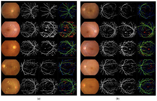
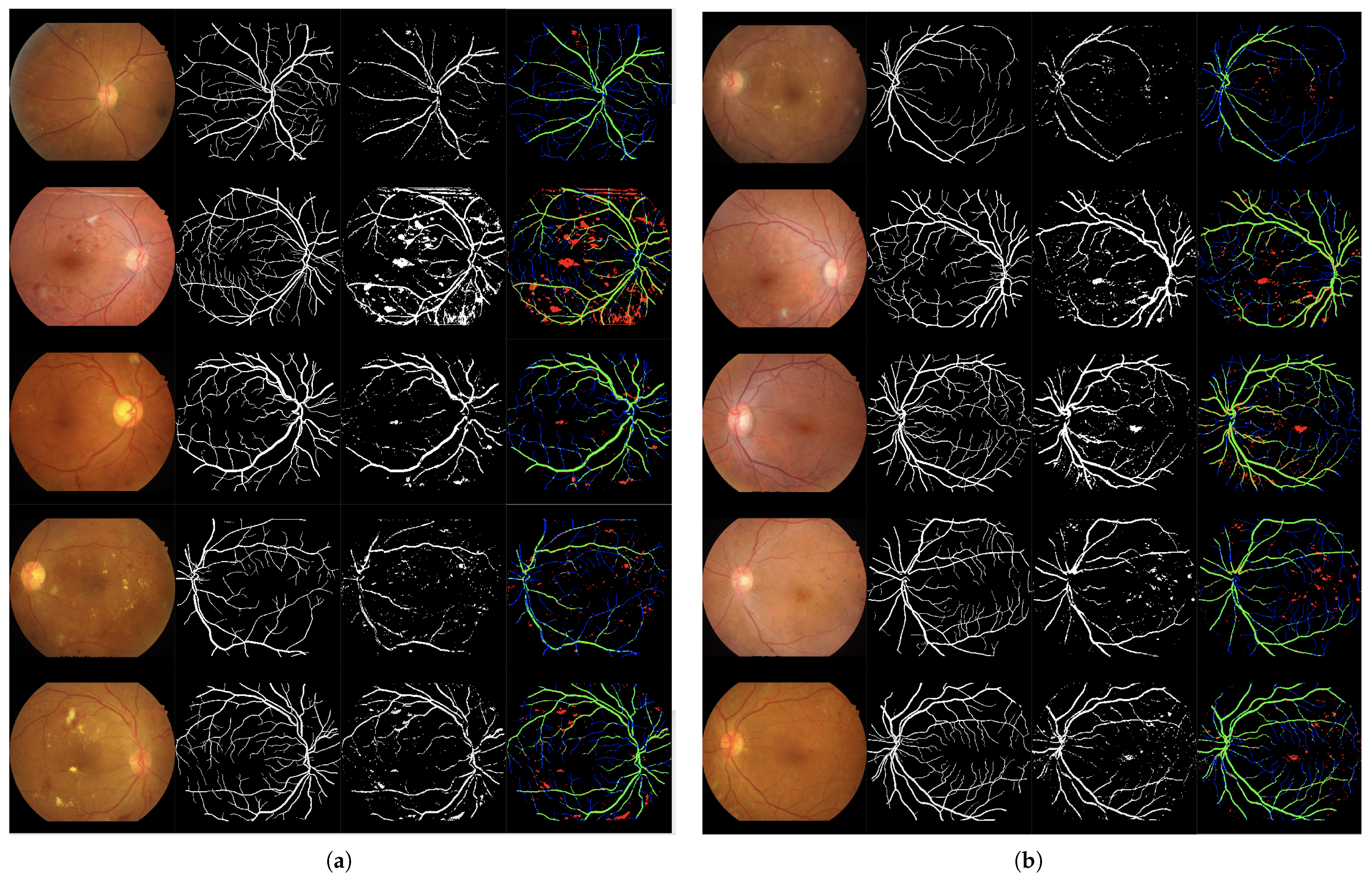
Figure 5.
Set of 4-image sequences illustrating the test results of Experiment 1 graphically. The first image is the original input, the second shows the ground truth vessel locations labeled by experts, the third corresponds to the output of the ANN from experiment 1, and the fourth visualizes the outcome in terms of true positives (green), false positives (red), false negatives (blue), and true negatives (black). Panel (a) displays the first five test images, while panel (b) shows the last five.
3.1.2. Experiment 2
Column-wise processing using a network based on Bi-directional LSTM and dropout layers. Solution I. Table 4 and Table 5 present the training and test results, respectively. Figure 6 presents the qualitative evaluation.
Table 4.
Extended classification metrics from Experiment 2, trained on the set of 44 images (IDRiD_01.jpg–IDRiD_44.jpg).
Table 5.
Extended classification metrics computed per image (rounded to two decimals), obtained during the test phase of Experiment 2.
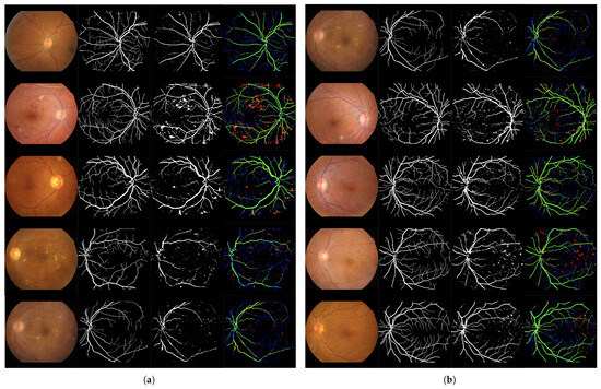
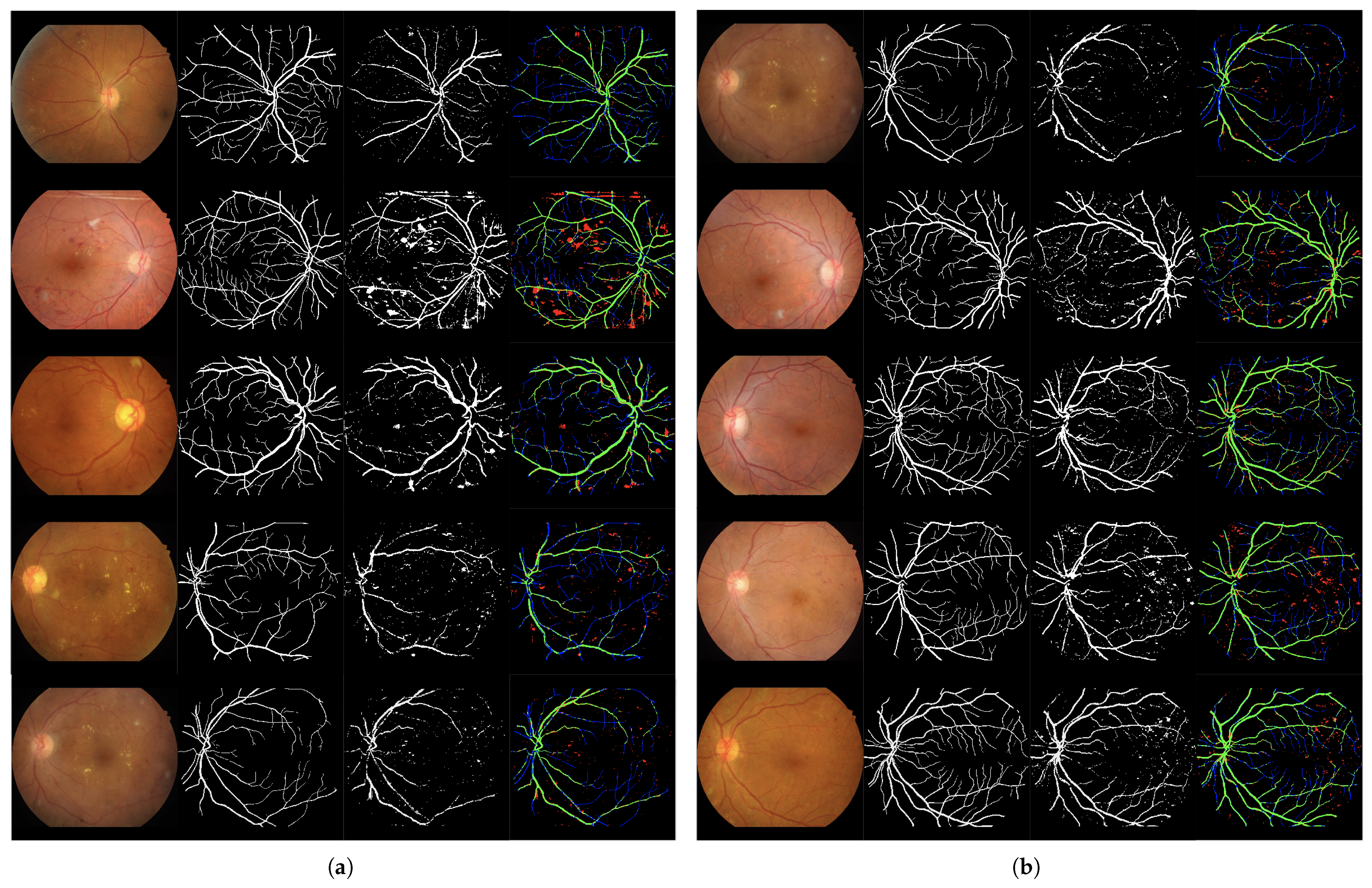
Figure 6.
Set of 4-image sequences illustrating the test results of Experiment 2 graphically. The first image is the original input, the second shows the ground truth vessel locations labeled by experts, the third corresponds to the output of the ANN from experiment 2, and the fourth visualizes the outcome in terms of true positives (green), false positives (red), false negatives (blue), and true negatives (black). Panel (a) displays the first five test images, while panel (b) shows the last five.
3.1.3. Experiment 3
Column-wise processing using a network based on Bi-directional LSTM and dropout layers. Solution II. Table 6 and Table 7 present the training and test results, respectively. Figure 7 presents the qualitative evaluation.
Table 6.
Extended classification metrics from Experiment 3, trained on the set of 44 images (IDRiD_01.jpg–IDRiD_44.jpg).
Table 7.
Extended classification metrics computed per image (rounded to two decimals), obtained during the test phase of Experiment 2.

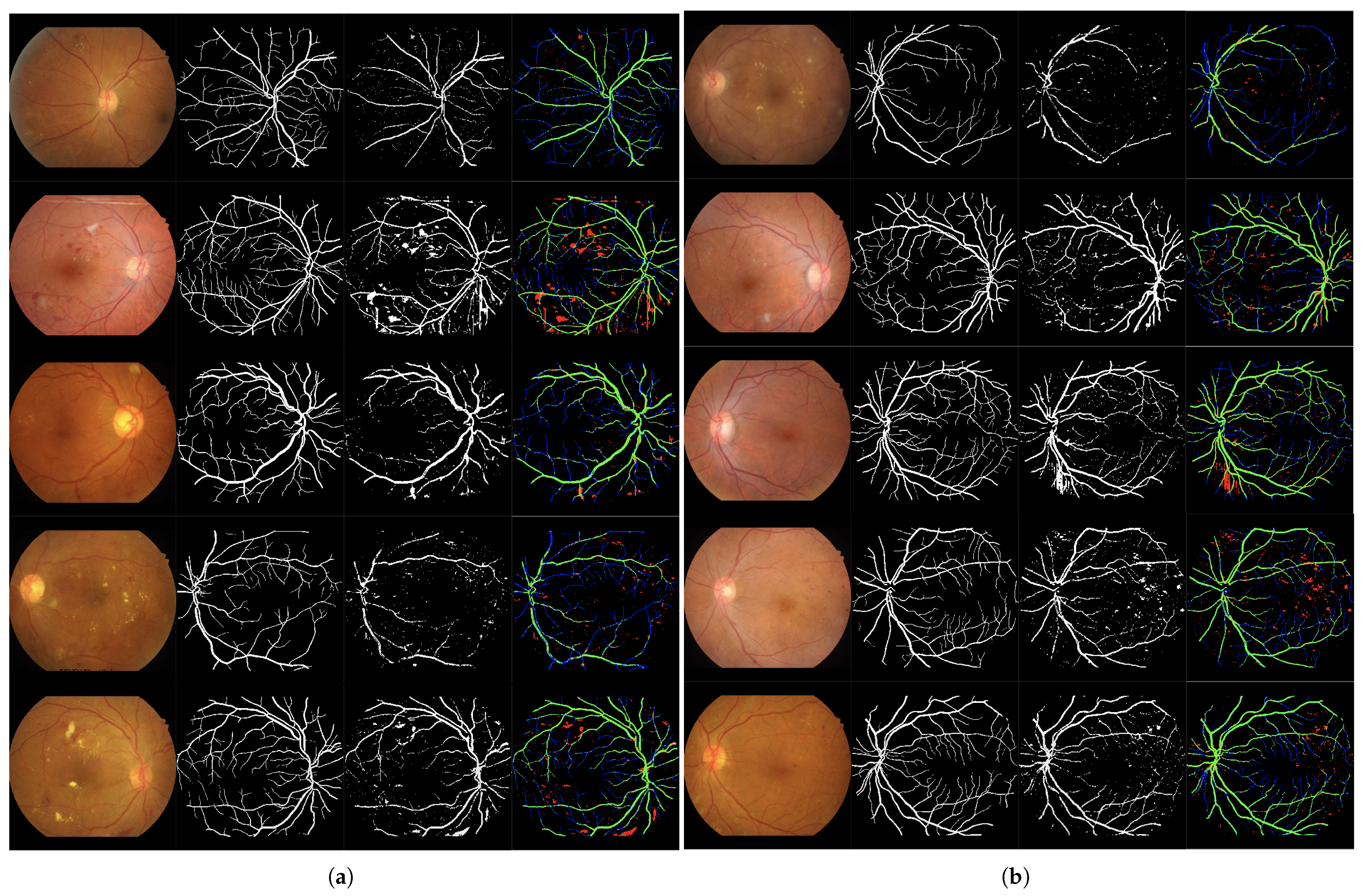
Figure 7.
Set of 4-image sequences illustrating the test results of Experiment 3 graphically. The first image is the original input, the second shows the ground truth vessel locations labeled by experts, the third corresponds to the output of the ANN from experiment 3, and the fourth visualizes the outcome in terms of true positives (green), false positives (red), false negatives (blue), and true negatives (black). Panel (a) displays the first five test images, while panel (b) shows the last five.
3.2. U-Net Baseline
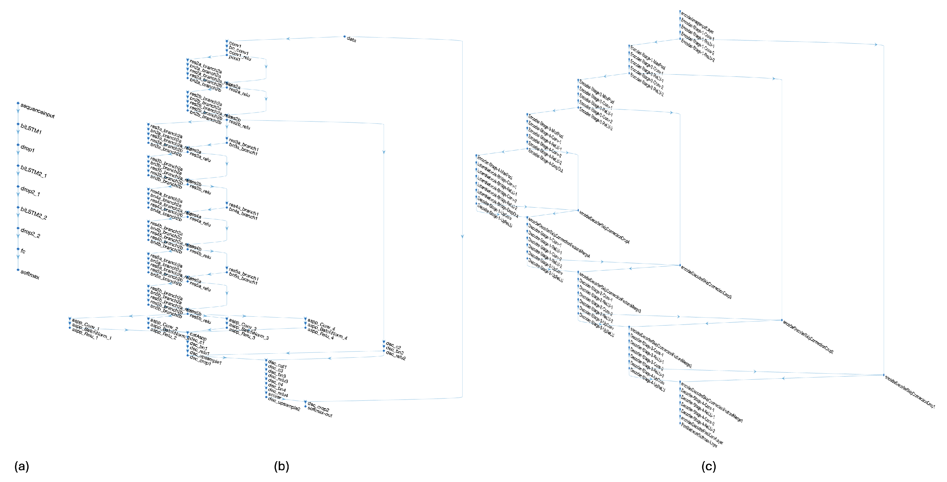
To benchmark the proposed Bi-LSTM against a standard CNN, we trained a 61-layer U-Net that processes full fundus images (architecture in Figure 8c).
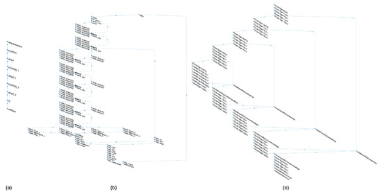
Figure 8.
Architecture of the neural network models tested, showing those that achieved the best performance in the evaluation. (a) The proposed approach based on Bi-directional LSTM layers; (b) the DeepLab v3+ network based on ResNet-18; and (c) the architecture based on a 2D U-Net model designed to process 1024 × 1024 × 3 input images.
Two variants were explored.
- (a)
- Plain—no data augmentation;
- (b)
- + Rotation augmentation—the same 15-angle policy used for the Bi-LSTM experiments.
The augmented U-Net attains 0.719 F1 with 34 M parameters (Table 8); the plain model is 0.07 F1 lower. Complete experimental details, including
Table 8.
Mean metrics for the U-Net baseline with rotation augmentation (Section 3.2).
- Training configuration (ADAM optimizer, 50 epochs);
- Metrics for both variants (plain and augmented);
- Per-image test results for all configurations.
are provided in Appendix A.
3.3. DeepLab v3+ Baseline
The ResNet-18 DeepLab v3+ (99 layers, 40 M parameters) improves F1 by +0.001 over U-Net but at 6× the parameter count of Bi-LSTM (Table 9). Full experimental details, including
Table 9.
Mean metrics for the DeepLab v3+ (ResNet-18) baseline (Section 3.3).
are provided in Appendix B.
3.4. ViT-Tiny Baseline
A lightweight ViT-Tiny encoder (5.72 M parameters) plus a four-stage U-Net decoder totals 6.1 M parameters, matching the Bi-LSTM scale. Despite the wider receptive field, ViT-Tiny lags the best Bi-LSTM by 0.207 F1 and doubles the false-positive rate (Table 10). Complete experimental details, including
Table 10.
Mean metrics for the ViT-Tiny baseline (Section 3.4).
- Architecture design (ViT-Tiny encoder + U-Net decoder);
- Training protocol (patch-based processing, AdamW optimizer);
- Qualitative error analysis.
are provided in Appendix C.
3.5. Global Comparison
Table 11 unifies the best Bi-LSTM and all three baselines on the most informative metrics, plus model size and pixel-wise inference speed. The proposed Bi-LSTM offers the highest F1/MCC at the lowest parameter count, validating sequence-first reasoning as a competitive alternative to both CNN and transformer designs.
Table 11.
Side-by-side comparison of the best Bi-LSTM versus all baselines.
4. Discussion
4.1. Principal Findings
This study demonstrates that a parameter-efficient, purely recurrent architecture can achieve competitive retinal vessel segmentation. The best Bi-LSTM configuration obtained a mean accuracy over 95.6% and a Matthews Correlation Coefficient (MCC) over 0.703 on the held-out RETA–IDRiD test subset (Table 5, Table 6 and Table 7). Notice that all of these results are obtained with no pre- or post-processing.
Our models exhibit a significantly lower number of trainable parameters, confirming their lightweight nature while maintaining competitive performance. Table 12 below summarizes the architectural complexity of the proposed Bi-LSTM variants compared to U-Net, DeepLab v3+, and ViT-Tiny.
Table 12.
Model architecture summary: U-Net, DeepLab, Bi-LSTM, and ViT-Tiny.
4.2. Methodological Contributions
- (a)
- Column-wise sample inflation. Decomposing every image into 1024 vertical sequences increased the effective training set from 44 to 45,056 instances without synthetic texture manipulation, supporting robust optimization on a limited corpus.
- (b)
- Transparent probability maps. The model outputs full-resolution 16-bit probability maps rather than hard binary masks. Releasing these logs alongside the code allows for exact reproduction of every metric in Table 3 and Table 5, Table 6 and Table 7 and facilitates independent error analysis (e.g., threshold sweeps, calibration curves or post hoc connectivity pruning) without rerunning training.
4.3. Limitations
- Dataset scope. All images originate from a single-camera model and demographic pool. Generalizability remains unverified; a planned external validation on the DRIVE and RVD datasets will be reported in a subsequent submission.
- Resolution constraints. The fixed 1024-pixel sequence length may degrade on ultra-wide-field fundus images; hierarchical or overlapping-window LSTMs will be explored.
- Absence of post-processing. Although deliberate, omitting morphological refinement marginally depresses the score relative to state-of-the-art CNN pipelines. A lightweight and connectivity-sensitive refinement module is in development.
4.4. Clinical Relevance
Accurate and computationally inexpensive vessel maps facilitate point-of-care applications, including automated arteriole-to-venule ratio (AVR) estimation and longitudinal microvascular monitoring in primary care settings. The low memory footprint positions the model for deployment on embedded retinal cameras.
Although current models have achieved very good segmentation performance, they still fall short of 100% accuracy, indicating that the problem remains open and subject to further improvement. At present, these models serve as diagnostic support tools in the clinical context. As observed in other fields, immediate improvements in these techniques are likely to come from the fusion of the outputs of multiple models. In this context, it is valuable to provide diverse approaches to the problem—whether through CNN-based networks, visual transformers, or slightly different strategies such as the one proposed in this work. These models should benefit from the integration of both classical image processing techniques—similar to the approaches described in [31,32]—and modern deep learning strategies, leveraging the strengths of each paradigm to enhance segmentation accuracy and robustness.
4.5. Future Work
- Post processing (1): Remove background artifacts—false positives, shown in red in Figure 5, Figure 6 and Figure 7—via object-based analysis. This leverages the morphological contrast between rounded blobs (artifacts) and elongated, thin structures (vessels) (see Figure 9a,b).
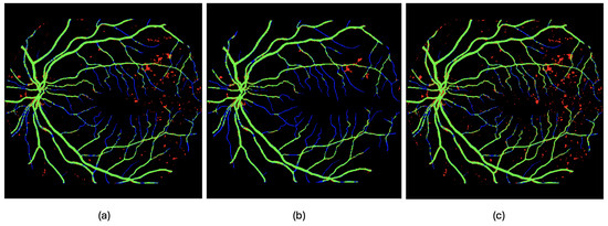 Figure 9. Examples of post-processing applied to the estimated output of image 54, with true positives (TPs) in green, false positives (FPs) in blue, false negatives (FNs) in red, and true negatives (TNs) in black. In (a), the segmentation output produced by the neural network from Experiment 2 on image 54 (the 10th image in the test set) is shown. In (b), a morphological filtering of the detected objects is performed based on their size and shape. In (c), a direct fusion (without the cleaning step) of the detections made by the network from Experiment 2 is shown, combining the outputs obtained from the original image orientation, as well as after rotations of 90 and 270 degrees, following realignment.
 - Post-processing (2): Improve true-positive detection using rotation-based inference. From qualitative inspection, it can be observed that processing the images column-wise prioritizes the detection of capillaries that evolve horizontally in the image, while hindering the detection of those oriented vertically—i.e., aligned with the direction of the columns. One way to enhance the detection of these vertically oriented capillaries is to apply 90-degree rotations to the image and reapply the method, thereby revealing structures that may have remained hidden. The method can be further improved by combining information obtained from multiple rotations, as certain capillaries that remain undetected in some regions may become visible under different orientations.The input image is rotated and processed multiple times, and then the outputs are realigned and aggregated to better capture fine vascular structures (see Figure 9a,c).
- Cross-device validation: evaluates the model on DRIVE, RVD, and other camera sources.
- Shallow CNN front-end: prepends a few convolutions to capture fine-scale texture before Bi-LSTM.
- Domain-shift mitigation: applies adversarial training so that precision is maintained in the new groups of patients.
- Ablation study: quantifies the impact of rotation policy, sequence length, and LSTM type before camera-agnostic release.
5. Conclusions
We propose a new approach to automated retinal vessel segmentation. The proposed solution processes the images in a column-wise manner. While the final solution to this task will likely involve a combination of different methods, introducing a conceptually distinct approach into the existing toolbox represents a meaningful contribution to the field. The results, obtained through three experiments, have been presented in raw form—without any pre- or post-processing—in order to clearly evaluate the potential of the proposed strategy.
Although a full-scale evaluation on the complete dataset has not yet been performed, preliminary observations suggest that post-processing involving the removal of false positives combined with multiple rotated inferences and realignment could significantly enhance segmentation performance. The proposed method supports an arbitrary number of inferences based on different image rotations, enabling the detection of small vessels from varying orientations.
It should also be noted that the models presented can be trained from scratch using a relatively small number of annotated images (44 in our case). This is a significant advantage compared to other methods, as image annotation requires highly specialized and labor-intensive manual work. So, some future work will focus on refining the post-processing pipeline and evaluating the method on a broader set of datasets, with the goal of developing a robust, lightweight solution suitable for real-world clinical deployment.
Author Contributions
Conceptualization, P.M.-P., K.M.K. and B.A.-M.; methodology, P.M.-P. and K.M.K.; software, P.M.-P. and K.M.K.; validation, P.M.-P., K.M.K. and B.A.-M.; formal analysis, P.M.-P., K.M.K. and B.A.-M.; investigation, P.M.-P. and K.M.K.; data curation, P.M.-P. and K.M.K.; writing—original draft preparation, P.M.-P. and K.M.K.; writing—review and editing, P.M.-P., K.M.K. and B.A.-M.; visualization, P.M.-P.; supervision, P.M.-P. and B.A.-M. All authors have read and agreed to the published version of the manuscript.
Funding
This research received no external funding.
Data Availability Statement
The dataset used in this study is publicly available; see Reference [12].
Conflicts of Interest
The authors declare no conflicts of interest.
Appendix A. U-Net Baseline Experiment Details
U-Net is a convolutional neural network architecture specifically designed for semantic segmentation tasks, particularly in biomedical image analysis. First introduced by Ronneberger et al. [33], U-Net has gained widespread adoption due to its ability to produce accurate pixel-level segmentations even when trained on relatively small datasets.
The architecture follows a symmetric encoder–decoder structure. The encoder path (also called the contracting path) captures the context of the image through successive convolution and pooling operations, reducing spatial dimensions while increasing feature depth. The decoder path (also called the expanding path) gradually recovers spatial information via upsampling and convolution, reconstructing a segmentation map with the original image resolution. A distinctive feature of U-Net is the use of skip connections between corresponding layers of the encoder and decoder. These connections concatenate feature maps from the contracting path with those in the expanding path, helping to preserve fine-grained details and improving localization accuracy. Due to its strong performance and architectural simplicity, U-Net has become a foundational model in medical image segmentation and continues to inspire a wide range of variants and extensions such as Attention U-Net [34], which incorporates attention gates that allow the network to focus on relevant regions of the image; the Nested U-Net [35], which enhances the original U-Net by introducing nested and dense skip pathways; or the ResUNet [36], which combines U-Net with residual learning to improve feature propagation and gradient flow.
In this experiment, we implement a U-Net architecture that operates directly on 1024 × 1024 × 3 images. The network consists of 61 layers, which are schematically illustrated in Figure 8c. The model was trained using the same dataset employed in the previous experiments. Once trained, it was tested on the same set of 10 test images, and the evaluation metrics were computed on a per-image basis to ensure reliable comparisons. Initially, the network was trained without data augmentation (see Table A1 and Table A2). Subsequently, a data augmentation strategy was applied by introducing rotations to the training images in order to ensure a processing scheme comparable to that used in the first three experiments (see Table A3 and Table A4). This strategy achieved the best results on the test set, although only slightly outperforming those obtained in Experiment 3.
Training Configuration
The U-Net model was trained using the ADAM optimizer, which combines momentum-based gradient descent with adaptive learning rate adjustment. The initial learning rate was set to , and no learning rate scheduling was applied throughout training. The optimizer’s hyperparameters included a gradient decay factor of 0.9 and a squared gradient decay factor of 0.999, with a small epsilon value () to ensure numerical stability. L2 regularization was applied with a weight of to reduce overfitting. Training was performed over a maximum of 50 epochs with a mini-batch size of 4. The training data was shuffled at the beginning of each epoch to enhance generalization. Validation was conducted every 50 iterations using the reserved validation set.
Table A1.
Extended classification metrics from U-Net, trained on the set of 44 images (IDRiD_01.jpg–IDRiD_44.jpg).
Table A1.
Extended classification metrics from U-Net, trained on the set of 44 images (IDRiD_01.jpg–IDRiD_44.jpg).
| NAME | Acc. (%) | TP (%) | TN (%) | FP (%) | FN (%) | R | S | P | F1 | FPR | MCC |
|---|---|---|---|---|---|---|---|---|---|---|---|
| means | 94.412 | 5.3561 | 89.056 | 2.561 | 3.027 | 0.63147 | 0.97206 | 0.68418 | 0.64806 | 0.027943 | 0.6429 |
Acc. = Accuracy, TP = True Positive, TN = True Negative, FP = False Positive, FN = False Negative, R = Recall, S = Specificity, P = Precision, = F1-Score, FPR = False-Positive Rate, MCC = Matthews Correlation Coefficient.
Table A2.
Extended classification metrics computed per image (rounded to two decimals), obtained during the test phase of U-Net.
Table A2.
Extended classification metrics computed per image (rounded to two decimals), obtained during the test phase of U-Net.
| NAME | Acc. (%) | TP (%) | TN (%) | FP (%) | FN (%) | R | S | P | F1 | FPR | MCC |
|---|---|---|---|---|---|---|---|---|---|---|---|
| IDRiD_45.jpg | 93.49 | 5.33 | 88.16 | 3.63 | 2.88 | 0.65 | 0.96 | 0.59 | 0.62 | 0.04 | 0.61 |
| IDRiD_46.jpg | 91.49 | 6.77 | 84.72 | 6.23 | 2.28 | 0.75 | 0.93 | 0.52 | 0.61 | 0.07 | 0.61 |
| IDRiD_47.jpg | 95.23 | 5.72 | 89.51 | 1.30 | 3.46 | 0.62 | 0.99 | 0.81 | 0.71 | 0.01 | 0.70 |
| IDRiD_48.jpg | 93.81 | 3.26 | 90.55 | 3.05 | 3.14 | 0.51 | 0.97 | 0.52 | 0.51 | 0.03 | 0.51 |
| IDRiD_49.jpg | 94.64 | 6.02 | 88.62 | 2.40 | 2.96 | 0.67 | 0.97 | 0.71 | 0.69 | 0.03 | 0.68 |
| IDRiD_50.jpg | 93.46 | 3.31 | 90.15 | 4.17 | 2.37 | 0.58 | 0.96 | 0.44 | 0.50 | 0.04 | 0.51 |
| IDRiD_51.jpg | 93.23 | 7.27 | 85.96 | 4.97 | 1.80 | 0.80 | 0.95 | 0.59 | 0.68 | 0.05 | 0.67 |
| IDRiD_52.jpg | 93.68 | 7.34 | 86.34 | 4.12 | 2.20 | 0.77 | 0.95 | 0.64 | 0.70 | 0.05 | 0.69 |
| IDRiD_53.jpg | 93.73 | 5.72 | 88.01 | 4.15 | 2.13 | 0.73 | 0.95 | 0.58 | 0.65 | 0.05 | 0.64 |
| IDRiD_54.jpg | 95.24 | 6.66 | 88.58 | 2.02 | 2.74 | 0.71 | 0.98 | 0.77 | 0.74 | 0.02 | 0.72 |
| means | 93.800 | 5.740 | 88.060 | 3.604 | 2.596 | 0.679 | 0.961 | 0.617 | 0.641 | 0.039 | 0.634 |
Acc. = Accuracy, TP = True Positive, TN = True Negative, FP = False Positive, FN = False Negative, R = Recall, S = Specificity, P = Precision, = F1-Score, FPR = False-Positive Rate, MCC = Matthews Correlation Coefficient.
Table A3.
Extended classification metrics from U-Net + DATA AUGMENTATION, trained on the set of 44 images (IDRiD_01.jpg–IDRiD_44.jpg).
Table A3.
Extended classification metrics from U-Net + DATA AUGMENTATION, trained on the set of 44 images (IDRiD_01.jpg–IDRiD_44.jpg).
| NAME | Acc. (%) | TP (%) | TN (%) | FP (%) | FN (%) | R | S | P | F1 | FPR | MCC |
|---|---|---|---|---|---|---|---|---|---|---|---|
| means | 95.777 | 4.549 | 91.227 | 0.746 | 3.476 | 0.563 | 0.991 | 0.855 | 0.677 | 0.008 | 0.682 |
Acc. = Accuracy, TP = True Positive, TN = True Negative, FP = False Positive, FN = False Negative, R = Recall, S = Specificity, P = Precision, = F1-Score, FPR = False-Positive Rate, MCC = Matthews Correlation Coefficient.
Table A4.
Extended classification metrics computed per image (rounded to two decimals), obtained during the test phase of U-Net + DATA AUGMENTATION.
Table A4.
Extended classification metrics computed per image (rounded to two decimals), obtained during the test phase of U-Net + DATA AUGMENTATION.
| NAME | Acc. (%) | TP (%) | TN (%) | FP (%) | FN (%) | R | S | P | F1 | FPR | MCC |
|---|---|---|---|---|---|---|---|---|---|---|---|
| IDRiD_45.jpg | 95.97 | 5.44 | 90.54 | 1.25 | 2.77 | 0.66 | 0.99 | 0.81 | 0.73 | 0.01 | 0.72 |
| IDRiD_46.jpg | 95.09 | 6.01 | 89.08 | 1.87 | 3.04 | 0.66 | 0.98 | 0.76 | 0.71 | 0.02 | 0.70 |
| IDRiD_47.jpg | 95.98 | 5.92 | 90.07 | 0.75 | 3.27 | 0.64 | 0.99 | 0.89 | 0.75 | 0.01 | 0.74 |
| IDRiD_48.jpg | 95.55 | 2.61 | 92.94 | 0.66 | 3.79 | 0.41 | 0.99 | 0.80 | 0.54 | 0.01 | 0.56 |
| IDRiD_49.jpg | 95.92 | 5.70 | 90.23 | 0.79 | 3.28 | 0.63 | 0.99 | 0.88 | 0.74 | 0.01 | 0.73 |
| IDRiD_50.jpg | 95.66 | 3.86 | 91.80 | 2.53 | 1.81 | 0.68 | 0.97 | 0.60 | 0.64 | 0.03 | 0.63 |
| IDRiD_51.jpg | 96.31 | 6.91 | 89.41 | 1.53 | 2.16 | 0.76 | 0.98 | 0.82 | 0.79 | 0.02 | 0.78 |
| IDRiD_52.jpg | 96.38 | 7.28 | 89.11 | 1.35 | 2.26 | 0.76 | 0.99 | 0.84 | 0.80 | 0.01 | 0.79 |
| IDRiD_53.jpg | 96.02 | 5.46 | 90.56 | 1.60 | 2.38 | 0.70 | 0.98 | 0.77 | 0.73 | 0.02 | 0.72 |
| IDRiD_54.jpg | 96.30 | 6.33 | 89.96 | 0.63 | 3.07 | 0.67 | 0.99 | 0.91 | 0.77 | 0.01 | 0.77 |
| means | 95.918 | 5.550 | 90.368 | 1.297 | 2.784 | 0.658 | 0.985 | 0.808 | 0.719 | 0.014 | 0.715 |
Acc. = Accuracy, TP = True Positive, TN = True Negative, FP = False Positive, FN = False Negative, R = Recall, S = Specificity, P = Precision, = F1-Score, FPR = False-Positive Rate, MCC = Matthews Correlation Coefficient.
Appendix B. DeepLab v3+ Baseline Experiment Details
The next baseline comparison is performed with a DeepLab v3+ convolutional neural network that performs well for semantic image segmentation. In this experiment, the DeepLab v3+ semantic segmentation network is also configured for input images of size 1024 × 1024 × 3 using ResNet-18 as the backbone encoder, which extracts hierarchical feature representations from the input image through successive convolutional and residual blocks providing a robust and semantically rich encoding.
ResNet-18 is a convolutional neural network that belongs to the family of Residual Networks (ResNets), introduced by He et al. [37]. It is widely used for image classification and as a feature extractor in various deep learning tasks. The core innovation of ResNet architectures is the use of residual learning, which addresses the problem of vanishing gradients in deep neural networks. ResNet-18 consists of 18 layers with learnable parameters, including convolutional layers, batch normalization, ReLU activation functions, and shortcut connections. These shortcut (or skip) connections enable the network to learn residual functions instead of directly learning unreferenced mappings. This design significantly improves training stability and allows for deeper networks to be optimized effectively.
The evaluated architecture configuration consists of 99 layers and is illustrated in Figure 8b. As in the previous experiments, the network was trained using the training image set, in this case employing the same data augmentation strategy as used in the second U-Net configuration of the preceding experiment. The model was then evaluated on the same set of 10 test images.
Training Configuration
The network was trained using the Stochastic Gradient Descent with Momentum (SGDM) optimizer. The training configuration included a momentum of 0.9 and an initial learning rate of 0.001, with a total of 60 epochs. No learning rate schedule was applied. Mini-batches of size 8 were used, and the data were shuffled at every epoch to improve generalization. L2 regularization was set to to prevent overfitting. Gradient thresholding was applied using the L2 norm method, with no explicit cap on the threshold (set to Inf).
Table A5.
Extended classification metrics in the training from DeepLab v3+ network based on ResNet-18, trained on the set of 44 images (IDRiD_01.jpg–IDRiD_44.jpg) with DATA AUGMENTATION.
Table A5.
Extended classification metrics in the training from DeepLab v3+ network based on ResNet-18, trained on the set of 44 images (IDRiD_01.jpg–IDRiD_44.jpg) with DATA AUGMENTATION.
| NAME | Acc. (%) | TP (%) | TN (%) | FP (%) | FN (%) | R | S | P | F1 | FPR | MCC |
|---|---|---|---|---|---|---|---|---|---|---|---|
| means | 96.287 | 5.550 | 90.736 | 0.880 | 2.832 | 0.653 | 0.990 | 0.861 | 0.740 | 0.009 | 0.737 |
Acc. = Accuracy, TP = True Positive, TN = True Negative, FP = False Positive, FN = False Negative, R = Recall, S = Specificity, P = Precision, = F1-Score, FPR = False-Positive Rate, MCC = Matthews Correlation Coefficient.
Table A6.
Extended classification metrics computed per image (rounded to two decimals), obtained during the test phase of DeepLab v3+ network based on ResNet-18.
Table A6.
Extended classification metrics computed per image (rounded to two decimals), obtained during the test phase of DeepLab v3+ network based on ResNet-18.
| NAME | Acc. (%) | TP (%) | TN (%) | FP (%) | FN (%) | R | S | P | F1 | FPR | MCC |
|---|---|---|---|---|---|---|---|---|---|---|---|
| IDRiD_45.jpg | 96.23 | 5.21 | 91.02 | 0.77 | 2.99 | 0.63 | 0.99 | 0.87 | 0.73 | 0.01 | 0.73 |
| IDRiD_46.jpg | 94.69 | 6.66 | 88.04 | 2.92 | 2.39 | 0.74 | 0.97 | 0.70 | 0.72 | 0.03 | 0.70 |
| IDRiD_47.jpg | 95.94 | 5.96 | 89.98 | 0.83 | 3.23 | 0.65 | 0.99 | 0.88 | 0.75 | 0.01 | 0.74 |
| IDRiD_48.jpg | 95.64 | 2.71 | 92.93 | 0.67 | 3.69 | 0.42 | 0.99 | 0.80 | 0.55 | 0.01 | 0.58 |
| IDRiD_49.jpg | 95.89 | 5.96 | 89.92 | 1.10 | 3.01 | 0.66 | 0.99 | 0.84 | 0.74 | 0.01 | 0.74 |
| IDRiD_50.jpg | 96.91 | 3.18 | 93.73 | 0.59 | 2.50 | 0.56 | 0.99 | 0.84 | 0.67 | 0.01 | 0.68 |
| IDRiD_51.jpg | 95.81 | 7.03 | 88.78 | 2.15 | 2.04 | 0.78 | 0.98 | 0.77 | 0.77 | 0.02 | 0.76 |
| IDRiD_52.jpg | 95.76 | 7.58 | 88.19 | 2.27 | 1.96 | 0.79 | 0.97 | 0.77 | 0.78 | 0.03 | 0.77 |
| IDRiD_53.jpg | 95.91 | 5.18 | 90.73 | 1.43 | 2.66 | 0.66 | 0.98 | 0.78 | 0.72 | 0.02 | 0.71 |
| IDRiD_54.jpg | 96.10 | 6.36 | 89.74 | 0.85 | 3.04 | 0.68 | 0.99 | 0.88 | 0.77 | 0.01 | 0.76 |
| means | 95.889 | 5.583 | 90.306 | 1.359 | 2.752 | 0.657 | 0.985 | 0.813 | 0.720 | 0.014 | 0.716 |
Acc. = Accuracy, TP = True Positive, TN = True Negative, FP = False Positive, FN = False Negative, R = Recall, S = Specificity, P = Precision, = F1-Score, FPR = False-Positive Rate, MCC = Matthews Correlation Coefficient.
Appendix C. Vision Transformer Baseline Experiment Details
Appendix C.1. Motivation and Related Work
Since the seminal Vision Transformer (ViT) paper by Dosovitskiy et al. [38], transformer backbones have displaced pure CNNs in many dense prediction tasks. Their global self-attention is particularly attractive for the analysis of retinal vessels, where long-range continuity cues complement local texture. Early medical hybrids such as TransUNet [39] and Swin-UNet [40] validated the concept on abdominal CT, and follow-up studies have transplanted similar designs to fundus imaging. For example, the region-based vision transformer RVT improves Dice by 1–3 pp over a deep U-Net on DRIVE, STARE and CHASE_DB1 [41], while Kim et al. fuse multi-scale ViT features with a connectivity-aware loss to obtain a 4–6 pp Dice uplift versus ResUNet [13]. Re-implementing these large models is impractical in our resource-constrained setting, so we instead adopt a minimal yet representative ViT-Tiny + U-Net decoder as the transformer baseline against which the proposed Bi-LSTM is benchmarked.
Appendix C.2. Architecture
We adopt vit_tiny_patch16_224 (5.7 M parameters, 12 transformer blocks each with three heads) as the encoder and attach a lightweight four-stage U-Net decoder (cf. TransUNet [39]). A 50% spatial dropout follows the decoder bottleneck, yielding a model with 6.1 M parameters—very close to the largest Bi-LSTM (6.4 M)—though the decoder does re-introduce standard convolutions.
Appendix C.3. Experimental Protocol
All hyper-parameters mirror the recurrent experiments: class-weighted cross-entropy, AdamW (, weight decay ) and the deterministic 44/10 RETA–IDRiD split. The images are tiled into overlapping windows (stride 200) because the resolution of the ViT patch is fixed at . Consequently, a single epoch sweeps ≈0.5 M patches—∼12× more gradient steps than one full-image epoch of the Bi-LSTM. During inference, softmax probabilities are stitched back to a single mask and thresholded at 0.5, exactly as for the Bi-LSTM pipeline.
Appendix C.4. Fairness Considerations
By holding the data split, augmentation policy, loss function, optimizer, and evaluation metrics constant, the transformer experiment provides an unbiased baseline for sequence-first versus attention-based reasoning. The sole caveat is the effective sample inflation caused by overlapping patches; this artifact is acknowledged when interpreting the results.
Appendix C.5. Quantitative Results
Average test-fold performance is summarized in Table A7; the metrics per image appear in Table A8. Despite the wider receptive field, ViT-Tiny trails the best Bi-LSTM by 0.21 in F1 and 0.12 MCC, and almost doubles the False-Positive Rate. Qualitative inspection attributes most false alerts to small exudates that the attention maps mistake for vessels, an error mode also reported by Kim et al. [13]. These findings reinforce our hypothesis that explicit sequence-first reasoning injects stronger connectivity priors than grid-based self-attention alone.
Table A7.
Average test-fold performance: best Bi-LSTM vs. ViT-Tiny.
Table A7.
Average test-fold performance: best Bi-LSTM vs. ViT-Tiny.
| Metric | Bi-LSTM | ViT-Tiny | |
|---|---|---|---|
| Accuracy (%) | 95.7 | 93.8 | |
| F1-score | 0.819 | 0.612 | |
| MCC | 0.697 | 0.580 | |
| FPR (%) | 1.2 | 2.9 |
Table A8.
Extended classification metrics computed per image for the ViT-Tiny baseline (12 epochs, identical protocol to Bi-LSTM).
Table A8.
Extended classification metrics computed per image for the ViT-Tiny baseline (12 epochs, identical protocol to Bi-LSTM).
| NAME | Acc. (%) | TP (%) | TN (%) | FP (%) | FN (%) | R | S | P | F1 | FPR | MCC |
|---|---|---|---|---|---|---|---|---|---|---|---|
| IDRiD_45 | 93.81 | 4.30 | 89.52 | 2.28 | 3.91 | 0.52 | 0.98 | 0.65 | 0.58 | 0.02 | 0.55 |
| IDRiD_46 | 92.38 | 4.84 | 87.54 | 3.41 | 4.21 | 0.53 | 0.96 | 0.59 | 0.56 | 0.04 | 0.52 |
| IDRiD_47 | 94.24 | 6.13 | 88.11 | 2.70 | 3.06 | 0.67 | 0.97 | 0.69 | 0.68 | 0.03 | 0.65 |
| IDRiD_48 | 95.20 | 3.12 | 92.07 | 1.53 | 3.28 | 0.49 | 0.98 | 0.67 | 0.57 | 0.02 | 0.55 |
| IDRiD_49 | 93.44 | 5.49 | 87.95 | 3.07 | 3.49 | 0.61 | 0.97 | 0.64 | 0.63 | 0.03 | 0.59 |
| IDRiD_50 | 95.56 | 3.23 | 92.33 | 2.00 | 2.44 | 0.57 | 0.98 | 0.62 | 0.59 | 0.02 | 0.57 |
| IDRiD_51 | 93.44 | 5.54 | 87.90 | 3.03 | 3.52 | 0.61 | 0.97 | 0.65 | 0.63 | 0.03 | 0.59 |
| IDRiD_52 | 92.69 | 5.28 | 87.41 | 3.05 | 4.26 | 0.55 | 0.97 | 0.63 | 0.59 | 0.03 | 0.55 |
| IDRiD_53 | 94.45 | 4.63 | 89.82 | 2.34 | 3.21 | 0.59 | 0.97 | 0.66 | 0.63 | 0.03 | 0.60 |
| IDRiD_54 | 93.69 | 6.33 | 87.37 | 3.23 | 3.08 | 0.67 | 0.96 | 0.66 | 0.67 | 0.04 | 0.63 |
| Means | 93.890 | 4.888 | 89.002 | 2.663 | 3.447 | 0.582 | 0.971 | 0.647 | 0.612 | 0.029 | 0.580 |
Acc. = Accuracy; TP = True Positive; TN = True Negative; FP = False Positive; FN = False Negative; R = Recall; S = Specificity; P = Precision; F1 = F1-Score; FPR = False-Positive Rate; MCC = Matthews Correlation Coefficient.
References
- Danielescu, C.; Dabija, M.G.; Nedelcu, A.H.; Lupu, V.V.; Lupu, A.; Ioniuc, I.; Gîlcă-Blanariu, G.-E.; Donica, V.-C.; Anton, M.-L.; Musat, O. Automated Retinal Vessel Analysis Based on Fundus Photographs as a Predictor for Non Ophthalmic Diseases—Evolution and Perspectives. J. Pers. Med. 2023, 14, 45. [Google Scholar] [CrossRef] [PubMed]
- Yau, J.W.Y.; Xie, J.; Lamoureux, E.; Klein, R.; Klein, B.E.K.; Cotch, M.F.; Bertoni, A.G.; Shea, S.; Wong, T.Y. Retinal microvascular calibre and risk of incident diabetes: The Multi-Ethnic Study of Atherosclerosis. Diabetes Res. Clin. Pract. 2012, 95, 265–274. [Google Scholar] [CrossRef] [PubMed]
- Ikram, M.K.; de Jong, F.J.; Bos, M.J.; Vingerling, J.R.; Hofman, A.; Koudstaal, P.J.; de Jong, P.T.V.M.; Breteler, M.M.B. Retinal Vessel Diameters and Risk of Stroke: The Rotterdam Study. Neurology 2006, 66, 1339–1343. [Google Scholar] [CrossRef] [PubMed]
- Wahlich, C.; Chandrasekaran, L.; Chaudhry, U.A.R.; Willis, K.; Chambers, R.; Bolter, L.; Anderson, J.; Shakespeare, R.; Olvera-Barrios, A.; Fajtl, J.; et al. Patient and Practitioner Perceptions around Use of Artificial Intelligence within the English NHS Diabetic Eye Screening Programme. Diabetes Res. Clin. Pract. 2025, 219, 111964. [Google Scholar] [CrossRef]
- Adamopoulou, M.; Makrynioti, D.; Gklistis, G.; Koutsojannis, C. A Comprehensive Overview of Deep Learning Techniques for Retinal Vessel Segmentation. Am. J. Biomed. Sci. Res. 2023, 19, 622–645. [Google Scholar] [CrossRef]
- Khanal, A.; Estrada, R. Dynamic Deep Networks for Retinal Vessel Segmentation. Front. Comput. Sci. 2020, 2, 35. [Google Scholar] [CrossRef]
- Galdran, A.; Anjos, A.; Dolz, J.; Lombaert, H. State-of-the-Art Retinal Vessel Segmentation with Minimalistic Models. Sci. Rep. 2022, 12, 6174. [Google Scholar] [CrossRef]
- Kande, G.B.; Nalluri, M.R.; Manikandan, R.; Rao, M.P.; Ramasamy, B. Multi-Scale Multi-Attention Network for Blood Vessel Segmentation in Fundus Images. Sci. Rep. 2025, 15, 3438. [Google Scholar] [CrossRef]
- Fadugba, J.; Köhler, P.; Koch, L.; Manescu, P.; Berens, P. Benchmarking Retinal Blood Vessel Segmentation Models for Cross-Dataset and Cross-Disease Generalization. arXiv 2024, arXiv:2406.14994. [Google Scholar]
- Shit, S.; Karaçay, E.; Navab, N. clDice++: Topology-Preserving and Uncertainty-Aware Loss for Medical Image Segmentation. Med. Image Anal. 2024, 88, 102899. [Google Scholar]
- Dulau, I.; Helmer, C.; Delcourt, C.; Beurton-Aimar, M. Ensuring a Connected Structure for Retinal Vessels Deep-Learning Segmentation. In Proceedings of the IEEE/CVF International Conference on Computer Vision Workshops (CVAMD @ ICCV), Paris, France, 2–3 October 2023; pp. 2364–2373. [Google Scholar]
- Lyu, X.; Cheng, L.; Zhang, S. The RETA Benchmark for Retinal Vascular Tree Analysis. Sci. Data 2022, 9, 15. [Google Scholar] [CrossRef] [PubMed]
- Kim, H.-J.; Eesaar, H.; Chong, K.T. Transformer-Enhanced Retinal Vessel Segmentation for Diabetic Retinopathy Detection Using Attention Mechanisms and Multi-Scale Fusion. Appl. Sci. 2024, 14, 10658. [Google Scholar] [CrossRef]
- Litjens, G.; Kooi, T.; Bejnordi, B.E.; Setio, A.A.A.; Ciompi, F.; Ghafoorian, M.; van der Laak, J.A.; van Ginneken, B.; Sánchez, C.I. A Survey on Deep Learning in Medical Image Analysis. Med. Image Anal. 2017, 42, 60–88. [Google Scholar] [CrossRef] [PubMed]
- Jin, K.; Huang, X.; Zhou, J.; Li, Y.; Yan, Y.; Sun, Y.; Zhang, Q.; Wang, Y.; Ye, J. FIVES: A Fundus Image Dataset for Artificial-Intelligence-Based Vessel Segmentation. Sci. Data 2022, 9, 141. [Google Scholar] [CrossRef]
- Li, M.; Huang, K.; Xu, Q.; Wang, S.; Li, T.; Chen, H.; Wang, Y.; Hu, L.; Shao, Y.; Deng, H.; et al. OCTA-500: A Retinal Dataset for Optical Coherence Tomography Angiography Study. arXiv 2022, arXiv:2012.07261. [Google Scholar] [CrossRef]
- Fraz, M.; Remagnino, P.; Barsi, A.; Hoppe, A.; Uyyanonvara, B.; Rudnicka, A.R.; Owen, C.G.; Barman, S.A. Blood-Vessel Segmentation Methodologies in Retinal Images—A Review. Comput. Methods Programs Biomed. 2012, 108, 407–433. [Google Scholar] [CrossRef]
- Mookiah, M.R.K.; Hogg, S.; MacGillivray, T.; Trucco, E. On the Quantitative Effects of Compression of Retinal Fundus Images on Morphometric Vascular Measurements in VAMPIRE. Comput. Methods Programs Biomed. 2021, 202, 105969. [Google Scholar] [CrossRef]
- Sun, X.; Fang, H.; Yang, Y.; Yuan, H.; Wang, J.; Yin, B. Robust Retinal Vessel Segmentation from a Data-Augmentation Perspective. arXiv 2021, arXiv:2007.15883. [Google Scholar]
- Desternes, J.; Lucas, C.; Vaysse, B.; Chapelle, K.; Robert, C.; Bloch, I.; Filliat, D.; Goutte, C. Medical Image Data Augmentation: Techniques, Comparisons and Interpretations. Artif. Intell. Rev. 2023, 56, 12561–12605. [Google Scholar] [CrossRef]
- Yavuz, Z.; Köse, Ç. Blood Vessel Extraction in Color Retinal Fundus Images with Enhancement Filtering and Unsupervised Classification. J. Healthc. Eng. 2017, 2017, 4897254. [Google Scholar] [CrossRef]
- Marti-Puig, P.; Serra-Serra, M.; Ribas, F.; Simarro, G.; Caballería, M. Automatic Shoreline Detection by Processing Plan-View Timex Images Using Bi-LSTM Networks. Expert Syst. Appl. 2024, 240, 122566. [Google Scholar] [CrossRef]
- Azad, R.; Asadi-Aghbolaghi, M.; Fathy, M.; Escalera, S. Bi-Directional ConvLSTM U-Net with Densely Connected Convolutions. In Proceedings of the IEEE/CVF International Conference on Computer Vision Workshops (ICCVW), Seoul, Republic of Korea, 27–28 October 2019. [Google Scholar]
- Porwal, P.; Pachade, S.; Kokare, M.; Deshmukh, G.; Sahasrabuddhe, V.; Meriaudeau, F.; Ren, H.; Li, H.; Bhandary, S.; Olson, J.; et al. Indian Diabetic Retinopathy Image Dataset (IDRiD): A Database for Diabetic Retinopathy Screening Research. Data 2018, 3, 25. [Google Scholar] [CrossRef]
- Staal, J.; Abramoff, M.D.; Niemeijer, M.; Viergever, M.A.; van Ginneken, B. Ridge-Based Vessel Segmentation in Color Images of the Retina. IEEE Trans. Med. Imaging 2004, 23, 501–509. [Google Scholar] [CrossRef] [PubMed]
- Hoover, A.; Goldbaum, M. Locating the Optic Nerve in a Retinal Image Using the Fuzzy Convergence of the Blood Vessels. IEEE Trans. Med. Imaging 2003, 22, 951–958. [Google Scholar] [CrossRef]
- Owen, C.G.; Rudnicka, A.R.; Mullen, R.; Bountziouka, V.; Whincup, P.H.; Cook, D.G.; Paterson, C.; McKay, G.J.; Clayton, G.; Hughes, A.D. Measuring Retinal Vessel Tortuosity in 10-Year-Old Children: Validation of the Computer-Assisted Image Analysis of Retina. Invest. Ophthalmol. Vis. Sci. 2016, 57, 685–691. [Google Scholar] [CrossRef]
- Cao, X.; Zhang, Y.; Zhao, X.; Cui, Z.; Li, Y.; Li, H.; Wang, Y.; Li, X. RVD: A Hand-Held Device-Based Fundus Video Dataset for Retinal Vessel Segmentation. In Advances in Neural Information Processing Systems 36: Datasets & Benchmarks Track; Casado, C., Mikolov, T., Eds.; Curran Associates: Red Hook, NY, USA, 2023. [Google Scholar]
- Touvron, H.; Cord, M.; Douze, M.; Massa, F.; Sablayrolles, A.; Jégou, H. Training Data-Efficient Image Transformers & Distillation through Attention. In Proceedings of the 38th International Conference on Machine Learning (ICML), Virtual Event, 18–24 July 2021; pp. 10347–10357. [Google Scholar]
- Wang, S.; Gao, J.; Li, Z.; Zhang, X.; Hu, W. A Closer Look at Self-Supervised Lightweight Vision Transformers. In Proceedings of the 40th International Conference on Machine Learning (ICML), Honolulu, HI, USA, 23–29 July 2023; pp. 37732–37745. [Google Scholar]
- Singh, P.P.; Garg, R.D. A hybrid approach for information extraction from high resolution satellite imagery. Int. J. Image Graph. 2013, 13, 1340007. [Google Scholar] [CrossRef]
- Putra, H.K.; Suprihatin, B. Retinal blood vessel extraction using a new enhancement technique of modified convolution filters and Sauvola thresholding. Int. J. Image Graph. 2023, 23, 2350006-1. [Google Scholar]
- Ronneberger, O.; Fischer, P.; Brox, T. U-Net: Convolutional Networks for Biomedical Image Segmentation. In Proceedings of the International Conference on Medical Image Computing and Computer-Assisted Intervention (MICCAI), Munich, Germany, 5–9 October 2015; pp. 234–241. [Google Scholar]
- Oktay, O.; Schlemper, J.; Folgoc, L.L.; Lee, M.; Heinrich, M.; Misawa, K.; Mori, K.; McDonagh, S.; Hammerla, N.Y.; Kainz, B.; et al. Attention U-Net: Learning Where to Look for the Pancreas. In Proceedings of the Medical Imaging with Deep Learning (MIDL), Amsterdam, The Netherlands, 4–6 July 2018. [Google Scholar]
- Zhou, Z.; Siddiquee, M.M.R.; Tajbakhsh, N.; Liang, J. UNet++: A Nested U-Net Architecture for Medical Image Segmentation. In Proceedings of the Deep Learning in Medical Image Analysis and Multimodal Learning for Clinical Decision Support (DLMIA), Granada, Spain, 16 September 2018; pp. 3–11. [Google Scholar]
- Zhang, Z.; Liu, Q.; Wang, Y. Road Extraction by Deep Residual U-Net. In Proceedings of the IEEE International Conference on Geoscience and Remote Sensing Symposium (IGARSS), Valencia, Spain, 22–27 July 2018; pp. 686–689. [Google Scholar]
- He, K.; Zhang, X.; Ren, S.; Sun, J. Deep Residual Learning for Image Recognition. In Proceedings of the IEEE Conference on Computer Vision and Pattern Recognition (CVPR), Boston, MA, USA, 7–12 June 2015; pp. 770–778. [Google Scholar]
- Dosovitskiy, A.; Beyer, L.; Kolesnikov, A.; Weissenborn, D.; Zhai, X.; Unterthiner, T.; Dehghani, M.; Minderer, M.; Heigold, G.; Gelly, S.; et al. An Image is Worth 16×16 Words: Transformers for Image Recognition at Scale. In Proceedings of the 9th International Conference on Learning Representations (ICLR), Virtual Event, 3–7 May 2021. [Google Scholar]
- Chen, J.; Lu, Y.; Yu, Q.; Luo, X.; Adeli, E.; Wang, Y.; Lu, L.; Yuille, A.L.; Zhou, Y. TransUNet: Transformers Make Strong Encoders for Medical Image Segmentation. arXiv 2021, arXiv:2102.04306. [Google Scholar]
- Cao, H.; Wang, Y.; Chen, J.; Jiang, D.; Zhang, X.; Tian, Q.; Wang, M. Swin-UNet: Unet-like Pure Transformer for Medical Image Segmentation. In Proceedings of the European Conference on Computer Vision (ECCV) Workshops, Tel Aviv, Israel, 23–27 October 2022. [Google Scholar]
- Zhang, Y.; Cao, X.; Zhao, X.; Lu, Y.; Zheng, Y. RVT: Reinforced Vision Transformer for End-to-End Retinal Vessel Segmentation. Med. Image Anal. 2023, 85, 102748. [Google Scholar]

Disclaimer/Publisher’s Note: The statements, opinions and data contained in all publications are solely those of the individual author(s) and contributor(s) and not of MDPI and/or the editor(s). MDPI and/or the editor(s) disclaim responsibility for any injury to people or property resulting from any ideas, methods, instructions or products referred to in the content. |
© 2025 by the authors. Licensee MDPI, Basel, Switzerland. This article is an open access article distributed under the terms and conditions of the Creative Commons Attribution (CC BY) license (https://creativecommons.org/licenses/by/4.0/).