Article

Leveraging Attribute Interaction and Self-Training for Graph Alignment via Optimal Transport

School of Computer Science and Technology, Beijing Jiaotong University, Beijing 100044, China
*
Author to whom correspondence should be addressed.
Mathematics 2025, 13(12), 1971; https://doi.org/10.3390/math13121971
Submission received: 13 May 2025 / Revised: 5 June 2025 / Accepted: 13 June 2025 / Published: 15 June 2025

Abstract

:
Unsupervised alignment of two attributed graphs finds the node correspondence between them without any known anchor links. The recently proposed optimal transport (OT)-based approaches tackle this problem via Gromov–Wasserstein distance and joint learning of graph structures and node attributes, which achieve better accuracy and stability compared to previous embedding-based methods. However, it remains largely unexplored under the OT framework to fully utilize both structure and attribute information. We propose an Optimal Transport-based Graph Alignment method with Attribute Interaction and Self-Training (PORTRAIT), with the following two contributions. First, we enable the interaction of different dimensions of node attributes in the Gromov–Wasserstein learning process, while simultaneously integrating multi-layer graph structural information and node embeddings into the design of the intra-graph cost, which yields more expressive power with theoretical guarantee. Second, the self-training strategy is integrated into the OT-based learning process to significantly enhance node alignment accuracy with the help of confident predictions. Extensive experimental results validate the efficacy of the proposed model.

1. Introduction

Given two attributed graphs G s and G t , the graph alignment problem finds the correspondence between the node sets of two graphs. It has numerous real-world applications, such as finding user identity matchings across social networks [1,2,3,4], aligning protein interaction networks [5,6,7], identifying common authors from different academic collaboration networks [8,9], and conducting entity alignment in various domains [10,11]. Existing studies of this problem can be categorized into supervised and unsupervised approaches, where the former [9,12,13] needs a set of matched node pairs (referred to as anchors) while the latter [14,15] conducts the alignment without any supervision. In cases where the anchors are hard to obtain, for example, subgraph counting [16] and structural alignment of molecules, we are motivated for unsupervised solutions only based on the similarities of graph structures and node attributes (i.e., node features).
One prominent category of unsupervised graph alignment approaches [13,17,18,19,20,21] adopts the idea of “Embed-Then-Cross-Compare” [14]. Specifically, the alignment is based on the explicitly learned node embeddings, and the goal is to minimize the distance of embeddings between the matched nodes. Representative methods (e.g., [17,22,23]) use graph neural networks (GNNs) to integrate both graph structures and node features to improve the expressiveness of node embeddings; for example, [17] employs adversarial training (GAN) [24] to minimize the distance between node pairs requiring alignment, while other approaches [22,23] achieve alignment through graph structure refinement. However, it is shown that directly aligning two embedding spaces without supervision is unstable and yields inferior performance [12].
Recently, a line of optimal transport (OT)-based methods [12,14,15] has been proposed for graph alignment, which demonstrates their advantages in prediction accuracy by formulating graph alignment as the OT problem. Generally speaking, given two probability distributions defined on the node sets, the OT algorithm (e.g., [25]) takes a non-negative cost function for node pairs as input and computes a probabilistic correspondence (referred to as the alignment matrix) so that the weighted total cost is minimized. Moreover, the alignment matrix must be a joint probabilistic distribution corresponding to the two marginal distributions for node sets. Therefore, the crux lies in the design of the cost function for node pairs, which is commonly implemented following the idea of Wasserstein distance (WD) [26] and Gromov–Wasserstein distance (GWD) [27]. It has been demonstrated that the specific choice of the cost function has a great impact on matching accuracy. For example, state-of-the-art performance is obtained by considering graph structures and node attributes jointly [14,15]. Nonetheless, we note that the idea of integrating structures and attributes into the OT framework is still in its infancy, leaving a large room for improving both model accuracy and efficiency.
In this paper, we focus on the unsupervised setting of graph alignment and propose an Optimal Transport-based Graph Alignment method with Attribute Interaction and Self-Training (PORTRAIT), which enhances the OT-based approaches from two perspectives. First of all, we observe that representative OT-based solutions (e.g., [14]) adopt attribute propagation (a.k.a. feature propagation) in the intra-graph cost design of the Gromov–Wasserstein learning process. More specifically, the feature embedding of each node is propagated to neighborhoods dimension by dimension, without interaction between different dimensions of node attributes. This leads to insufficient information exchange when two attribute dimensions have similar semantics. In contrast, our model employs a learnable linear transformation layer after feature propagation, which yields more expressive power with theoretical guarantee and still guarantees provable convergence. Meanwhile, to integrate richer graph structures and information, we aggregate the outputs of all convolutional layers into node embeddings, as each layer captures distinct hidden features from both local and global perspectives. Superior matching accuracy is achieved in the empirical study, coinciding with our theoretical analysis.
Second, the intra-graph cost represents the interactions between nodes within a single graph, and it plays a crucial role in determining matching accuracy [14]. By analyzing the variability of interaction strength among nodes in intra-graph cost, we can categorize nodes as either easier or harder to match. Using nodes with higher matching confidence as pseudo-labels, we propose a self-training strategy with our refined cost computation process that leverages structural-based node similarities to enhance existing OT-based methods. Our contributions are summarized as follows.
  • We propose an unsupervised learning approach for graph alignment under the framework of Gromov–Wasserstein distance and optimal transport. Compared to existing OT-based methods, deeper graph structures and node information are incorporated in the design of the intra-graph cost, meanwhile, linear transformation of node attributes is integrated into cost design to facilitate attribute interaction across dimensions. It is proved to have more expressive power while sharing the convergence results. Moreover, we introduce a cost normalization layer to enhance the stability of model training.
  • Inspired by the global interaction properties of nodes reflected in the intra-graph cost, by selecting high-confidence matched node pairs as pseudo-labels, we propose a self-training strategy that not only enhances our model but also improves the accuracy of other OT-based methods.
  • Extensive experimental results demonstrate PORTRAIT’s outstanding performance, achieving a 5% improvement in Hits@1, while also exhibiting remarkable efficiency and robustness.

2. Preliminary

2.1. Problem Definition

We formally define the unsupervised graph alignment problem. Particularly, an undirected attributed graph G of n nodes is associated with the adjacency matrix A { 0 , 1 } n × n and node attribute matrix X R n × d . A i j is set to 1 if there is an unweighted edge between the i-th and j-th nodes.
Definition 1
(Unsupervised Graph Alignment). Given a pair of graphs G s = ( V s , E s ) and G t = ( V t , E t ) with adjacency matrices A p and node features X p ( p = { s , t } ), we need to predict a set of aligned (i.e., matched) node pairs { ( u i , v k ) | u i V s , v k V t } without any observed correspondence, where u i and v k are corresponding nodes across two graphs.
Note that for the supervised setting of the problem, we additionally have a set of known matchings between two graphs which are referred to as anchors, and need to predict the matchings for the remaining nodes. In this paper, we focus on the optimal transport-based solutions for graph alignment as they achieve state-of-the-art performance for both supervised (e.g., [12]) and unsupervised settings (e.g., [14,15]). We briefly introduce the optimal transport problem.
Definition 2
(Optimal Transport  (OT) Problem). We are given two distributions μ and ν on two finite sets X and Y , and a cost function C : X × Y R . We have | X | = n 1 and | Y | = n 2 . Kantorovich’s formulation of the optimal transport problem finds a solution T * such that
T * = inf T Π ( μ , ν ) x = 1 n 1 y = 1 n 2 C ( x , y ) T ( x , y ) = inf T Π ( μ , ν ) C , T .
where Π ( μ , ν ) denotes all possible joint distributions with the corresponding marginals equal to μ and ν. We use C R n 1 × n 2 and T R n 1 × n 2 to represent the cost and alignment matrix, respectively.
In practice, the OT problem is typically solved with entropic constraints for better efficiency [25]. Specifically, a regularization term is introduced (with λ > 0 ):
T * = inf T Π ( μ , ν ) C , T λ h ( T ) .
where h ( T ) = i , k T ( i , k ) log T ( i , k ) is the entropy of T . The solution to Equation (2) has the form of
T * = D i a g ( a ) exp ( C λ ) D i a g ( b ) .
In particular, a and b are adjustable vectors depending on each other, while T * has a unique solution as the objective is convex [25]. Note that we have i , k T ( i , k ) = 1 because it is a joint probability distribution, while T ( i , k ) is mostly determined by C ( i , k ) and they are in reverse correlation.
Without loss of generality, let n 1 = | V s | and n 2 = | V t | ; we assume that n 1 n 2 . To predict the correspondence between V s and V t following almost all previous works, for each u i V s , we choose M ( u i ) = argmax v k T ( i , k ) , where M ( u ) (resp. M ( v ) ) is the matched vertex of u (resp. v) in the other graph.
Table 1 lists the frequently used notations throughout the paper.

2.2. State-of-the-Art Methods

We discuss the representative methods for graph alignment under both unsupervised and supervised settings and include them as the main competitors of our approach.

2.2.1. Unsupervised Graph Alignment

Representative methods for the unsupervised setting can be roughly divided into two categories. One category [13,17,18,19,20,21] follows the idea of “Embed-Then-Cross-Compare”, i.e., they first generate embeddings for all nodes in both graphs and then seek a solution to minimize the distance between those embeddings of matched nodes.
  • WAlign [17]: The algorithm first employs lightweight graph neural networks (GNNs), e.g., [28], to compute the embedding z u of each node u, and then treats unsupervised graph alignment as minimizing the following objective:
    M * = argmin | M | = n 1 ( u i , v k ) M z u i z v k .
The above equation can be interpreted as the Wasserstein distance (WD) [26]. Thus, inspired by Wasserstein GAN [24], WAlign proposes a GAN-based framework, where the discriminator minimizes u i V s f w ( z u i ) v k V t f w ( z v k ) . The 1-Lip-schitz function f w is implemented by a neural network, based on which the pseudo corresponding node pairs are generated. The parameters of the GNN are updated by a similar loss function with an additional reconstruction term.
  • GAlign [22]: The model incorporates the idea of data augmentation into the learning objective to obtain high-quality node embeddings. In particular, it encourages the node embeddings Z p ( k ) ( p = s , t ) of each GNN layer k to retain graph structures, as well as to be robust upon graph perturbation. Afterward, the alignment refinement procedure augments the original graph by first choosing the confident node matchings and then increasing the weight of their adjacency edges. This serves as an effective unsupervised heuristic to iteratively match node pairs.
  • GTCAlign [23]: Arguably having the best accuracy among embedding-based solutions, it simplifies the idea of GAlign with the following observation. First, it uses a GNN with randomized parameters for node embedding computation, as it is intricate to design an embedding-based objective that directly corresponds to the goal of node alignment. Second, the iterative learning process is empowered by graph augmentation, i.e., to adjust edge weights according to confident predictions. By normalizing the node embeddings to length 1, the learning process gradually decreases the cosine angle between confident node matchings.
Another recent line of research [12,14,15,29,30] adopts optimal transport for graph alignment, which finds a probabilistic matching between two distributions on graphs and demonstrates better accuracy and robustness.
  • GWL [15]: Xu et al. [15] present a graph matching framework by combining the graph-based optimal transport and node embedding learning. It predicts an alignment matrix T following Definition 2. Given the learnable node representations Z s R n 1 × d and Z t R n 2 × d , GWL minimizes a combination of the Wasserstein discrepancy and the Gromov–Wasserstein discrepancy (GWD), while the latter shares similar ideas with graph matching. Specifically, the objective for the Wasserstein discrepancy is L w d = K ( Z s , Z t ) , T , where K ( · , · ) is a function to measure the distance based on two node embeddings. The loss corresponding to the Gromov–Wasserstein discrepancy is defined as
    L g w d = C g w d , T = L ( C s ( Z s ) , C t ( Z t ) , T ) , T ,
    where the form of L R n 1 × n 2 follows GWD:
    L ( C s , C t , T ) ( i , k ) = u j G s v l G t ( C s ( i , j ) C t ( k , l ) ) 2 T ( j , l ) .
For GWL, the forms of intra-graph cost matrices  C s and C t are hand-engineered, which is a combination of the adjacency information and the cosine distance based on node embeddings.
Intuitively, Equation (6) states that if ( u i , v k ) and ( u j , v l ) are two matched pairs, the distance between u i and u j in G s (i.e., C s ( i , j ) ) is close to the distance between v k and v l in G t (i.e., C t ( k , l ) ). Note that the matched pairs suggest a large value of T ( i , k ) (and T ( j , l ) ), indicating that L ( C s , C t , T ) ( i , k ) is small. Consequently, the intra-graph costs need to be close, which establishes the correspondence between graph topologies. GWL leverages the proximal point method [31] to convert the GWD objective to an OT problem and alternatively learns the alignment matrix T and node embeddings Z s and Z t . The convergence is theoretically guaranteed [15].
  • SLOTAlign [14]: As the state-of-the-art unsupervised method, SLOTAlign improves existing GWD-based approaches (e.g., [15,32]) with a more careful design of the intra-graph costs C s and C t . It introduces the module of multi-view structure modeling which incorporates graph structure, node features, and multi-hop information via an attribute propagation procedure. Then, it uses a few learnable parameters (with additional constraints) to compute the intra-graph cost from the weighted sum of the above information. Next, SLOTAlign adopts a similar procedure as GWL to learn the alignment matrix T by minimizing GWD (see Equation (5)).

2.2.2. Supervised Graph Alignment

Given a set of anchors as input, supervised graph alignment methods mostly focus on how to fully exploit the anchor information and propagate it to nearby nodes. Random Walk with Restart (RWR)-based solutions are widely adopted [9,13,33] while the very recent work [12] integrates the idea of label propagation with optimal transport.
  • PARROT [12]: Given a set of anchors that Q = { ( x k , y k ) , k [ 1 , q ] } with x k G s and y k G t , PARROT first generates the position-aware node embeddings for both graphs. For each anchor node x k (resp. y k ), it computes the RWR (a.k.a. Personalized PageRank, PPR [34]) vector on G s (resp. G t ):
    r k ( p ) = ( 1 α ) W p r k ( p ) + α e k ( p ) , p = s , t .
Here, W p = A p D p 1 represents the transition matrix, with D p being the diagonal degree matrix. The parameter α is referred to as the teleportation probability [34] and e k ( p ) is a one-hot vector with the x k -th (resp. y k -th) component to be 1. By concatenating all the vectors to get the n 1 × q -sized R s = ( r 1 ( s ) , , r q ( s ) ) and the n 2 × q -sized R t = ( r 1 ( t ) , , r q ( t ) ) , each node in G s and G t obtains a q-dimensional positional embedding. Then, the inter-graph cost matrix C r w r is computed by a two-step procedure:
C b a s e = α e R s R t + ( 1 α ) e X s X t .
v e c ( C r w r ) = ( 1 δ ) γ W s t v e c ( C r w r ) + ( 1 + δ ) v e c ( C b a s e ) .
To be more precise, it first computes a base case matrix C b a s e by comparing the positional embeddings as well as node attributes of two graphs, and then conducts an RWR-based propagation on the product graph G s G t (i.e., conducting the Kronecker product on A s and A t ). Both δ and γ are adjustable parameters, and v e c ( C ) concatenates all the columns of C into an n 1 n 2 -dimensional vector.
With the inter-graph cost C r w r , PARROT transforms graph alignment to the OT problem, which is similar to GWL and SLOTAlign. The minimization of both WD and GWD is considered along with a few consistency regularization terms.

3. Our Approach

3.1. Model Overview

As demonstrated in Figure 1, our model is composed of three major phases. The attribute propagation and interaction phase takes graph structures (i.e., A ) and node attributes (i.e., X ) as input and computes the node embedding matrix Z , which is then used to improve the cost computation in the following phase and to enhance model accuracy. The unsupervised Gromov–Wasserstein learning phase utilizes Gromov–Wasserstein distance [27] to address the issue of non-comparability arising from inconsistent graph topologies [14,15]. Both phases are combined to form an end-to-end pipeline that predicts the alignment matrix T . Next, the self-training phase is applied to compute a revised prediction T to improve the matching accuracy and it can be applied to other existing OT-based methods (e.g., [14,15]). The pseudo-code is demonstrated in Algorithm 1, with the details of three phases described in the following subsections. Note that for each node u i in the smaller graph G s , the algorithm returns u i with its matched node M ( u i ) , where M ( u i ) is the node in G t with the largest matching probability T ( i , k ) .
Algorithm 1: PORTRAIT.
Input: Two attributed graphs G s and G t with A s , X s , A t , and X t
Output: The set of predicted node matchings
// Algorithm 2
Z p AttrProp   &   Interact ( A p , X p ) , p = { s , t } ;
// Algorithm 3
T Unsuper - GW ( A s , X s , Z s , A t , X t , Z t ) ;
// Algorithm 4
T Self - Training ( T , A s , X s , A t , X t ) ;
return { ( u i , M ( u i ) ) M ( u i ) = argmax v k T ( i , k ) , u i V s } ;

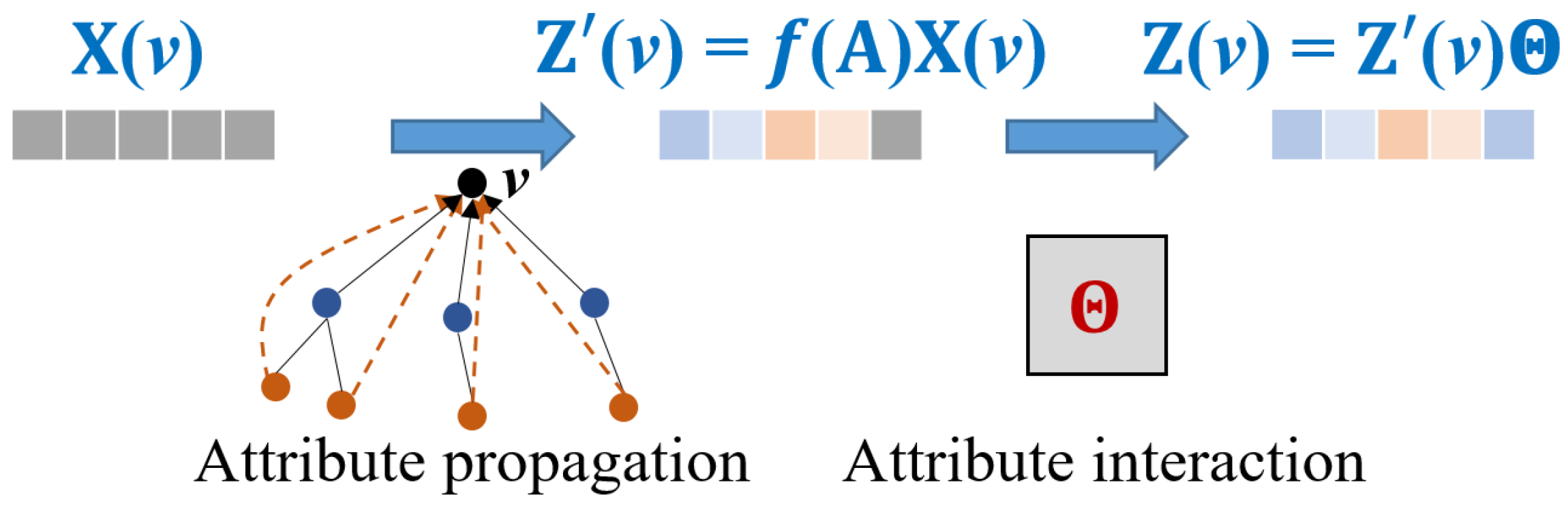
3.2. Attribute Propagation and Interaction

Compared to representative OT-based solutions [14,15], we add a preliminary step named attribute propagation and interaction in Figure 2 to enhance the cost computation of the next GW learning phase. As pointed out by [14], the alignment quality via OT heavily depends on the specific design of two intra-graph cost matrices. Given a graph G, let X ( v ) R d denote node v’s attribute. State-of-the-art solution [14] adopts the subgraph-view structure modeling process, which can be formulated as attribute propagation:
Z ( v ) = f ( A ) X ( v ) ,
where A is the adjacency matrix of G, and f ( A ) denotes the general transformation of A . Specifically, it uses the following equation for propagation with k [ 1 , K ]  [14]:
f ( A ) = D ˜ 1 2 A ˜ D ˜ 1 2 k ,
where A ˜ = A + I and D ˜ is the diagonal matrix representing the degree of A ˜ (i.e., D ˜ = diag ( A ˜ 1 ) ). To this end, for each dimension i of node v’s representation Z ( v ) , Z ( v , i ) is augmented with the dimension-wise information of its k-hop neighbors.
However, two dimensions of the node attribute might have similar semantics, for example, when attributes are encoded in one-hot manner. In this case, it is reasonable to unify both dimensions in the latent space. Attribute propagation is incapable of encouraging information exchange across different dimensions of the node attributes. We propose an additional attribute interaction step with a learnable transformation matrix Θ R ( K + 1 ) d × d :
Z ( v ) = Z ( v ) Θ .
As Z ( v , i ) represents the linear combination of all the feature dimensions of Z ( v ) , we implement the information exchange not only between different attributes of v but also between those of v and its k-hop neighbors. Although the solution is simple, it theoretically improves the expressive power of the Gromow–Wasserstein learning phase (see Section 3.3) and results in better matching accuracy in practice. The pseudo-code is shown in Algorithm 2.   
Algorithm 2: AttrProp&Interact.
Input: Adjacency matrix A and node attributes X
Output: Node representation Z
// Attribute Propagation
Z ( v ) f ( A ) X ( v ) ;
// Attribute Interaction
Z ( v ) Z ( v ) Θ ;
return  Z ( v ) ;

3.3. Unsupervised Gromov–Wasserstein Learning

3.3.1. Cost Computation

We first describe the cost computation steps of the Gromov–Wasserstein (GW) learning framework (see Figure 3). Following existing approaches [14,15], we have intra-graph cost computation followed by inter-graph cost computation.
  • Intra-graph cost computation. We adopt the multi-view modeling of intra-graph cost, which considers graph structure A , node attributes X , and a joint modeling of them via node representation Z :
    C p = β 1 ( p ) · A p + β 2 ( p ) · X p X p + β 3 ( p ) · Z p Z p , p = s , t
    where C s R n 1 × n 1 and C t R n 2 × n 2 denote the intra-graph cost matrix of G s and G t , respectively. Here, we use β ( p ) = ( β 1 ( p ) , β 2 ( p ) , β 3 ( p ) ) to represent the learnable coefficients. Compared to [14], we compute Z through both attribute propagation and interaction (see Section 3.2), while simultaneously aggregating node representations from different convolutional layers to capture both local and global information, which enhances the model’s expressiveness (as demonstrated in Theorem 1). Specifically, it has the following concrete form:
    f ( A p , X p ) = Concat ( X p , W p X p , , W p K X p ) , Z p = Dropout ( σ ( f ( A p , X p ) ) ) Θ .
We use W to represent the normalized adjacency matrix, i.e., W = D ˜ 1 2 A ˜ D ˜ 1 2 , and σ ( · ) denotes the activation function. Following our discussion in Section 3.2, Θ R ( K + 1 ) d × d is the learnable transformation matrix in the attribute interaction step.
  • Inter-graph cost computation. Given intra-graph cost matrices C s and C t , this step follows the definition of Gromow–Wasserstein discrepancy (Equation (6)). We denote by C g w d the n 1 × n 2 -sized inter-graph cost matrix.
The following theorem states the discriminative power of our cost design backed by attribute propagation and interaction.
Theorem 1.
For the computation of the Gromov–Wasserstein discrepancy, with attribute interaction, the constructed intra-graph cost matrix has more discriminative power than when only attribute propagation is applied.
Proof. 
Let M * denote the ground truth node matching and assume that ( u i , v k ) , ( u j , v k ) M * and ( u j , v k ) M * . By the interpretation of GW discrepancy, C s ( i , j ) and C t ( k , l ) should be similar [14], say, | C s ( i , j ) C t ( k , l ) | < ε 1 . Meanwhile, we should also have | C s ( i , j ) C t ( k , l ) | ε 2 with ε 2 > ε 1 .
Now, consider the case d i s t ( u i , u j ) > K , d i s t ( u i , u j ) > K , and X s ( u i ) X s ( u j ) = X s ( u i ) X s ( u j ) = 0 , for example; they are all one-hot vectors taking the values of 1 at different dimensions. Here, d i s t ( · , · ) is the shortest distance between two nodes. Then, the first two terms of C s ( i , j ) and C s ( i , j ) are 0 (see Equation (13)). Moreover, as u i and u j (resp. u j ) are with more than k-hops, after propagation of the one-hot attributes, we still have the third term Z s ( u i ) Z s ( u j ) = Z s ( u i ) Z s ( u j ) = 0 , where Z s = f ( A s ) X s . Consequently, we have | C s ( i , j ) C t ( k , l ) | = | C s ( i , j ) C t ( k , l ) | = | C t ( k , l ) | ; that is, the cost design cannot discriminate the matched pair ( u j , v k ) and unmatched node pair ( u j , v k ) .
With attribute interaction, it is possible to learn the transformation matrix Θ so that Z s ( u i ) Z s ( u j ) = Z s ( u i ) Θ Θ Z s ( u j ) 0 even if Z s ( u i ) Z s ( u j ) = 0 , which also holds for u j . For the same reason, it is possible to have | C s ( i , j ) C t ( k , l ) | | C s ( i , j ) C t ( k , l ) | , and the theorem follows.    □
Our cost computation differs from representative GW learning approaches [14,15] in the following aspects. We provide a more flexible multi-view modeling which enables a full interaction of graph structures and node attributes. Meanwhile, we take a step further to include attribute interaction, enhancing the model’s expressive power.
  • Cost normalization. It has been observed that the Sinkhorn algorithm [25] invoked by the GW learning process might have numerical instability issues [35]. We observe that most terms ( C s ( i , j ) C t ( k , l ) ) 2 are far less than 1 in practice. As the average value of T ( j , l ) is 1 n 1 n 2 , the inter-graph cost for most node pairs are of very small values. We find that this phenomenon deteriorates the stability of GW learning. Hence, we employ a cost normalization module to rescale the inter-graph cost. Let C m a x = max i , k C g w d ( i , k ) and C m i n = min i , k C g w d ( i , k ) , we have
    C g w d ( i , k ) C g w d ( i , k ) C m i n C m a x C m i n , i , k .
Note that after normalization, all the elements of C g w d fall into [ 0 , 1 ] .

3.3.2. Learning Algorithm

We employ the widely used proximal point method [31,36] in existing OT-based solutions [12,14,15] to learn the parameters Θ = { β ( s ) , β ( t ) , Θ } and the alignment matrix T . It optimizes Θ and T alternatively with an iterative procedure. In particular, the objective is
min Θ , T C g w d , T = min T ( μ , ν ) i , j , k , l C s ( i , j ) C t ( k , l ) 2 T ( i , k ) T ( j , l ) . s . t . T 1 = μ , T 1 = ν , T ( i , k ) 0 .
The pseudo-code of unsupervised GW learning is shown in Algorithm 3. We first initialize β ( s ) , β ( t ) , and T as uniform distribution and randomly initialize Θ (Line 1). For each iteration (Line 2), we compute the intra-graph cost (Lines 3) followed by the inter-graph cost (Line 4). Next, the normalization trick is applied (Line 5). We then invoke [31,36] to learn { β ( s ) , β ( t ) , Θ } and T (Line 6).
Algorithm 3: Unsuper-GW.
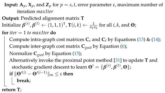
Mathematics 13 01971 i001
We demonstrate that with the newly added parameters Θ in the attribution interaction step, under mild assumptions, Algorithm 3 can still converge. We have the following theorem, which is extended from the theoretical results of [14].
Theorem 2.
Let F ( T , β , Θ ) denote the learning objective in Equation (16), with β = ( β ( s ) , β ( t ) ) . Suppose that 0 < τ T < 1 L f T , 0 < τ β < 1 L f β , and 0 < τ Θ < 1 L f Θ , where L f T , L f β , and L f Θ are the gradient Lipschitz continuous modulus of F ( T , β , Θ ) , respectively. Then, with the condition in Equations (18)–(20), any limit point of the sequence ( T ( i ) , β ( i ) , Θ ( i ) ) i 0 converges to a critical point of F ¯ ( T , β , Θ ) , with
F ¯ ( T , β , Θ ) = F ( T , β , Θ ) + I T ( T ) + I B ( β ) + I W ( Θ ) ,
where I ( · ) denotes the indicator function. Specifically, we have
T = { T 0 : T 1 = μ , T 1 = ν } ,
B = { ( β ( s ) , β ( t ) ) 0 : i = 1 3 β i ( p ) = 1 , p = s , t } ,
W = { Θ 0 : i = 1 ( K + 1 ) d Θ i j = 1 , j [ 1 , d ] } .
Proof. 
Our proof generally follows that of Theorem 5 in [14]. Note that by our definition, T , B , and W are bounded sets, and F ( T , β , Θ ) is a bi-quadratic function with respect to T , β , and Θ . To guarantee that Θ satisfies the above constraint, in each iteration, it is sufficient to apply an activation (e.g., ReLU) function followed by column-wise normalization. The proof then follows Theorem 5 in [14], where we can compute the gradient of F w.r.t. T , β , and Θ to update the parameters with provable convergence.    □
  • Relaxing the constraints on  β , Θ . Through our empirical study, we find that the constraints on β (as in [14]) and Θ (see Theorem 2) can be relaxed. That is, we do not force the non-negativity of parameters nor constrain that the (column-wise) summation equals 1. Please note that the theoretical analysis only guarantees convergence of the algorithm to a critical point, which aligns with the existing studies [14,15].

3.4. Self-Training Phase

We illustrate the self-training phase in Figure 4. It includes a pseudo-anchor selection step followed by the similarity-based cost propagation (SCP) procedure, which is used to enhance the state-of-the-art supervised method [12] for graph alignment.

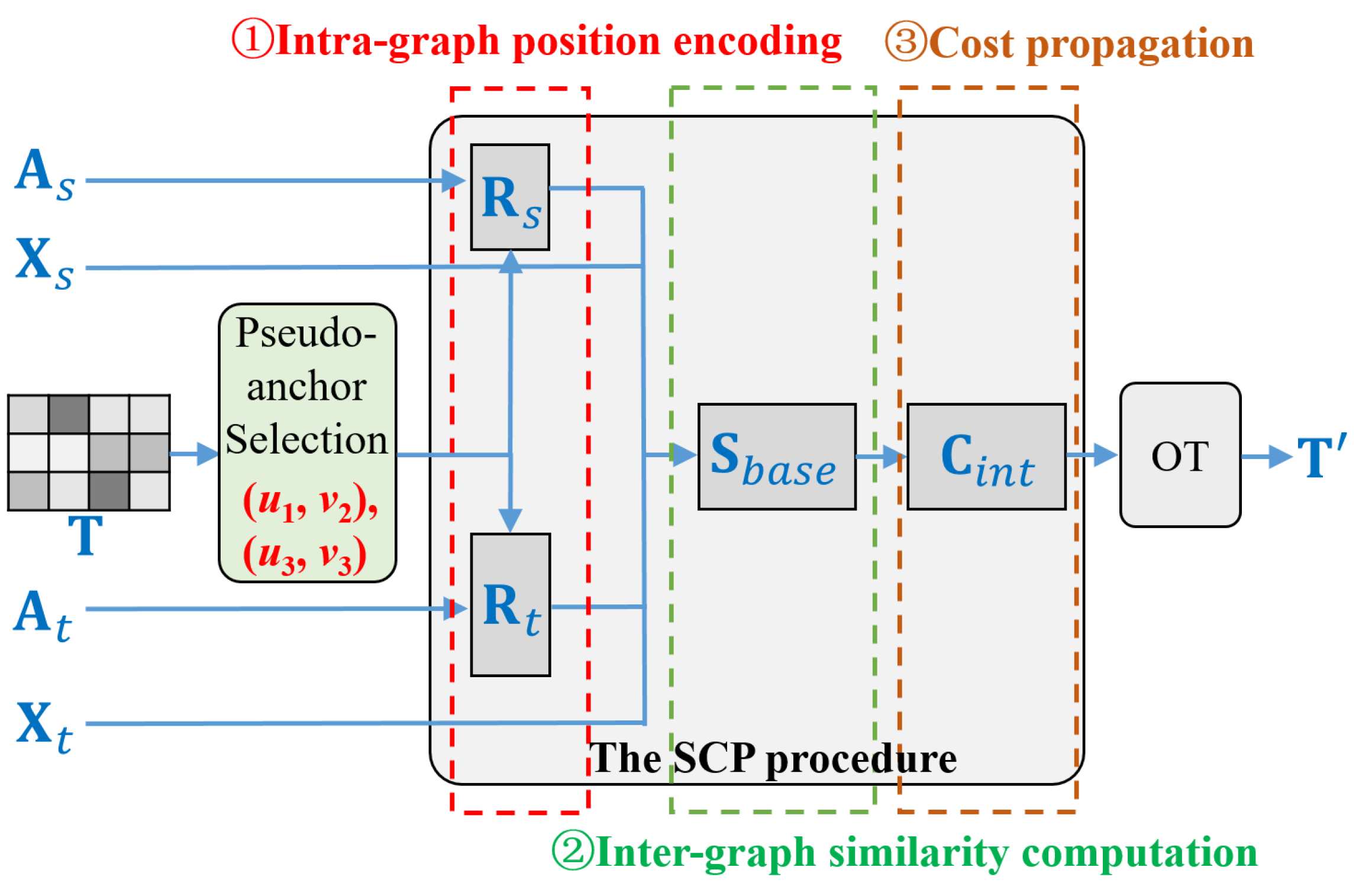
3.4.1. Pseudo-Anchor Selection

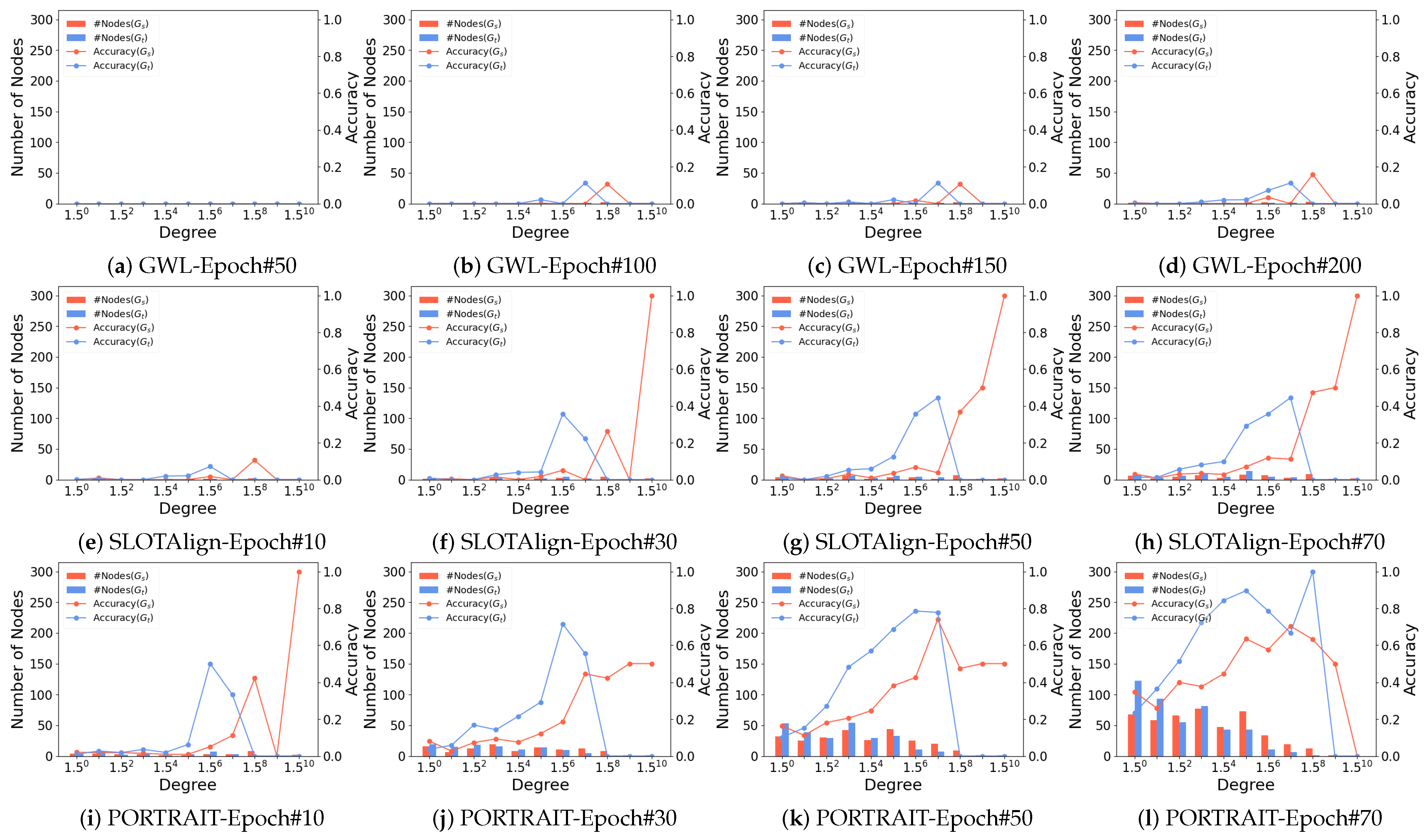
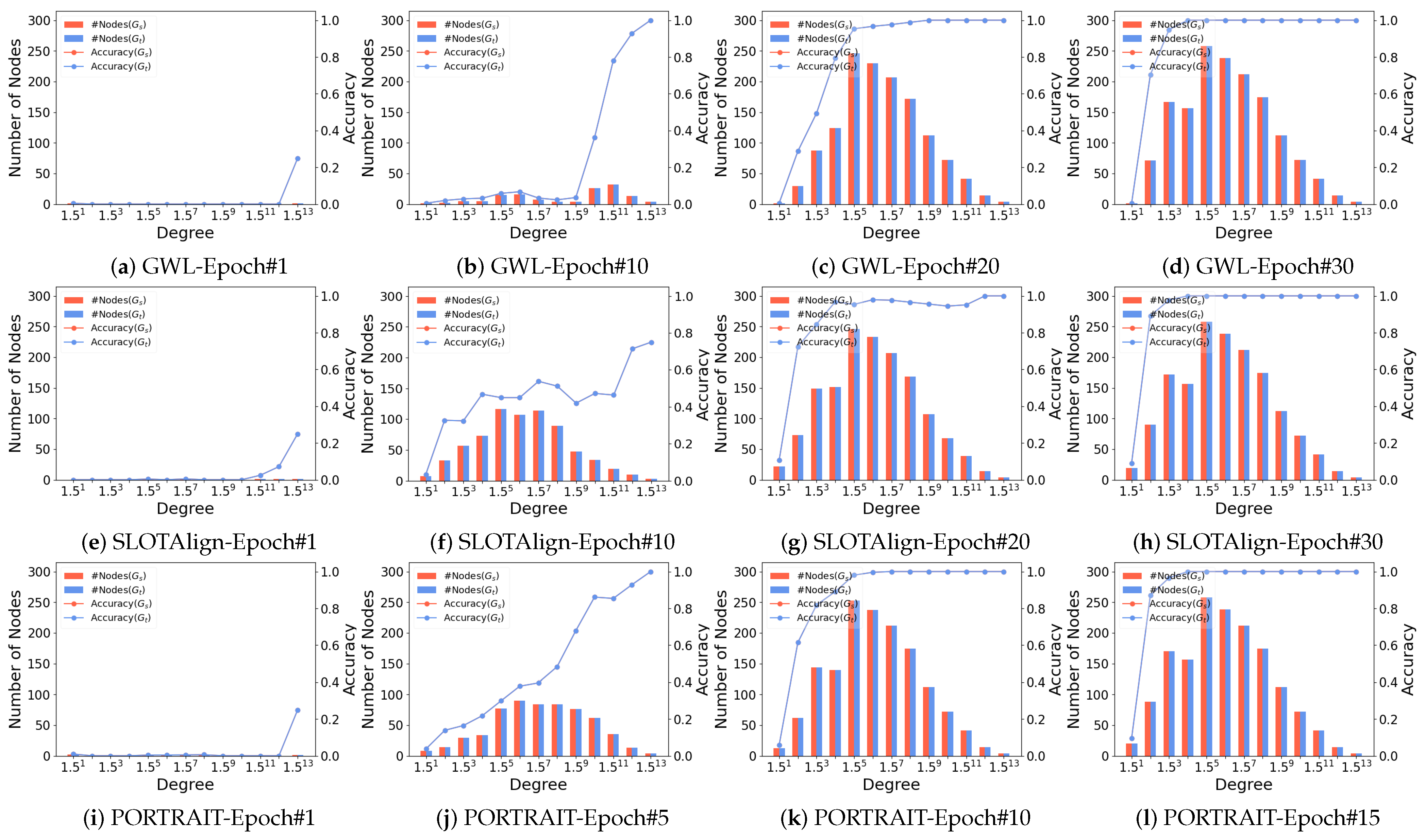
  • Motivation. As mentioned above, when using Gromov–Wasserstein distance (GWD) to model the graph alignment problem, C p represents the intra-graph cost, C p R n × n , p = s , t , which is crucial for determining the matching accuracy [14], as it captures the relationships between nodes within a single graph. In this context, for a graph with n nodes, we can categorize the nodes into those that are easy to match and those that are more challenging to align. A natural question that arises is how to define which nodes are more likely to be matched accurately. Since C p represents the dependencies between nodes, a fundamental metric node degree can provide insight. Nodes with higher degree can access more information across the graph, capturing dependencies with multiple other nodes, which aligns well with C p role in representing overall intra-graph relationships. Conversely, nodes with a lower degree are relatively less capable of modeling inter-node relationships, making them harder to align accurately.
Based on the above analysis, we employ various OT-based methods [14,15] across different datasets to examine the node-matching process in detail. We observe that nodes with higher degrees are matched more accurately, which is consistent with our analysis. Take SLOTAlign [14] and two widely used datasets, Douban Online–Offline [33] and ACM-DBLP [37], as an example. As shown in Figure 5, we place nodes into bins corresponding to degrees in [ θ i , θ i + 1 ) for i = 0 , , log θ d m a x . We set θ = 1.5 to scatter the nodes so that they do not gather in few bins (we also remove bins that only contain less than 1% of all nodes). The red (resp. blue) bars denote the number of correctly aligned nodes in G s (resp. G t ) for each bin, while the red (resp. blue) lines show the corresponding prediction accuracy (i.e., Hits@1). It is clear that nodes with top degrees (e.g., top-10% to 30% nodes) have a significantly higher accuracy than the remaining nodes. Moreover, we also note that these nodes in G s (resp. G t ) tend to have large values of max k T ( i , k ) (resp. max i T ( i , k ) ), namely, the values in the i-th row (resp. k-th column) are more concentrated given that their summations are fixed.
The above observation motivates us to present a self-training strategy as follows. First, a set of matched nodes with high accuracy is selected as the pseudo-anchors. Second, we use a supervised graph alignment solution modified by our SCP approach, leveraging the pseudo-anchors for supervision to refine the input alignment matrix T .
To be more precise, given the alignment matrix T obtained in the unsupervised learning phase and a predefined pseudo-anchors ratio defined by the hyperparameter q, we sort the value of { ( u i , max k T ( i , k ) ) | u i G s } by descending the order of max k T ( i , k ) and select the top-q node pairs ( u i , M ( u i ) ) as pseudo-anchors (it is also fine to first select nodes v k in G t and then find their matching nodes in G s ). In practice, we usually set q [ 0.1 , 0.3 ] .

3.4.2. Similarity-Based Cost Propagation (SCP)

During the self-training phase, we enhance the existing OT-based method, PARROT [12], to serve as the supervised model. We find that the positional embedding and the inter-graph cost computation of [12] is suboptimal (see Equations (8) and (9)). To be specific, for any two nodes u i G s and v k G t with close positional embeddings (i.e., R s ( i ) R t ( k ) ) or similar features (i.e., X s ( i ) X t ( k ) ), the value of C b a s e ( i , k ) is small. In other words, C b a s e denotes the node-wise distances across graphs, where matrix components with small values carry more information (and they are few in numbers according to the sparse nature of graph alignment). However, as Equation (9) essentially represents the RWR-based node similarity propagation on the product graph G s G t in which C b a s e is regarded as the personalized vector [34], these small-valued components have minor effects in propagation. Particularly, v e c ( C b a s e ) can be decomposed into
v e c ( C b a s e ) = C b a s e ( 1 , 1 ) · e 1 + + C b a s e ( n 1 , n 2 ) · e n 1 n 2 ,
where C b a s e ( i , k ) denotes the component at i-th row and k-th column, and e s is an n 1 n 2 -dimensional one-hot vector with the s-th element being 1. It is clear that similar node pairs with small C b a s e ( i , k ) s contribute less to the propagation results C r w r .
Instead, we adopt a node-wise similarity-based approach to conduct the propagation, which is referred to as similarity-based cost propagation (SCP). We first define the node-wise similarity rather than the distances as the base case:
S b a s e = α e τ ( R s R t 1 ) + ( 1 α ) e τ ( X s X t 1 ) .
where τ > 0 is a temperature parameter. Note that for normalized R s ( i ) , R t ( k ) , X s ( i ) , and X t ( k ) , we have S b a s e ( i , k ) [ e 2 τ , 1 ] . Next, the inter-graph cost with supervision, C i n t is computed as Equation (23):
v e c ( C i n t ) = ( 1 δ ) γ W s t v e c ( C i n t ) + ( 1 + δ ) ( 1 n 1 n 2 v e c ( S b a s e ) ) .
We elaborate on the meaning of C i n t as Equation (24). According to the definition of RWR (i.e., PPR [34]), we have
vec ( C i n t ) = ( I ( 1 δ ) γ W s t ) 1 ( 1 + δ ) × ( 1 n 1 n 2 vec ( S b a s e ) ) = i = 0 ( 1 + δ ) ( 1 δ ) i γ i W s t i 1 n 1 n 2 i = 0 ( 1 + δ ) ( 1 δ ) i γ i W s t i vec ( S b a s e ) .
Note that the second term of Equation (24) is the RWR propagation with personalized vector v e c ( S b a s e ) . Therefore, it corresponds to node-wise similarity propagation on G s G t . To transform the similarities into distances, we subtract it from the first term, which refers to the propagation with an all-one vector. Another choice is to compute the inter-graph similarities S r w r , which equals to the second term of Equation (24). Next, we compute C i n t = max ( 1 n 1 1 n 2 S r w r , 0 n 1 × n 2 ) . This gives comparable or slightly inferior results compared to Equation (23). If it holds that S b a s e ( i , k ) 1 for all i and k, we have C i n t 0 n 1 × n 2 .

3.4.3. Learning Algorithm

As shown in Algorithm 4, we first conduct pseudo-anchor selection (Line 1), followed by similarity-based cost propagation (Line 2). We then conduct supervised OT-based learning, for example, by invoking [12] with the refined inter-cost (Line 3), and use the refined alignment matrix T to update our prediction (Line 4), including the pseudo-anchor nodes.
  • Remark. In principle, our self-training process can be used to improve any existing OT-based unsupervised methods such as [14,15].
Algorithm 4: Self-training.
Input: The alignment matrix T obtained from the unsupervised step, the ratio of pseudo-anchors q
Output: The refined alignment matrix T
Sort { ( u i , max k T ( i , k ) ) | u i G s } by descending order of max k T ( i , k ) and select the top- q % node pairs as pseudo-anchors;
Compute the node-wise similarities (Equation (22)) and the inter-graph cost (Equation (23));
Replacing the original transport cost in PARROT [12] with SCP to obtain a refined alignment matrix T ;
return  T ;

3.5. Complexity Analysis

We present a concise complexity analysis of PORTRAIT. Consider source graph G s has n s nodes and m s edges while target graph G t has n t nodes and m t edges, and the feature dimension is d. Defining n = max ( n s , n t ) , the computational requirements are as follows:
Intra-graph Cost Computation: The construction of cost matrices C s and C t in Equation (13) requires O ( n 2 d ) operations, as established in [14,15]. Evaluating the GW term in Equation (6) dominates the complexity with O ( n 3 ) operations. This complexity governs both the β -update and T -update steps in Equation (16). Given the typical condition d min ( n s , n t ) , the total complexity reduces to O ( n 3 ) , maintaining parity with existing optimal transport-based alignment methods [14,15,32].
Note that the computational bottleneck originates from the Gromov–Wasserstein learning process, which employs proximal gradient methods [31,36] for alignment matrix updates. While this complexity is inherent to current OT-based graph alignment approaches, we recognize that scalability remains an important unresolved challenge that will be prioritized in our future research.

4. Experimental Analysis

4.1. Experimental Setup

  • Datasets: Three widely-used datasets for attributed graph alignment [9,12,14,17] are adopted, which contain information on graph structures and node features (see Table 2).
Douban Online–Offline [33] contains two social networks corresponding to an online graph and an offline graph of Douban users. Node features denote user locations. The larger online graph contains all the users in the offline graph.
The ACM-DBLP [37] dataset contains two academic collaboration networks extracted from ACM and DBLP, respectively. Nodes represent authors while edges represent collaborations. The numbers of papers published in venues (of four research areas) are used as node features.
The Allmv-Imdb [22] dataset contain two networks. The Allmv network is derived from the Rotten Tomatoes website, where two films are connected by an edge if they share at least one common actor. The Imdb network is constructed from the Imdb website using a similar approach. The alignment indicates film identity, incorporating 5174 anchor links.
PPI [38] is a semi-synthetic dataset where two different node permutations of a protein interaction network are generated. We mainly use it to demonstrate the important properties of OT-based approaches in an adversarial setting where the motivation of self-training is less obvious. Note that this dataset is much easier than the two real datasets as all baselines achieve high accuracy.
  • Baselines: We include representative embedding-based methods WAlign [17], GAlign [22], and GTCAlign [23], and use GWL and SLOTAlign as the OT-based competitors because they achieve state-of-the-art performance on the aforementioned datasets according to [14,15]. We do not include [32,39,40] as baselines since they are significantly outperformed by GWL and SLOTAlign [14] and thus are not comparable with ours. We also omit [29,30] as they are limited to graphs with no larger than one hundred nodes. For all baselines, we run the code provided by the authors with the default configuration.
  • Evaluation Metrics: We evaluate the performance of all models using the well-adopted metric Hits@k with k { 1 , 5 , 10 } . Hits@k indicates whether the ground truth correspondence of a node occurs in the top-k predictions ordered by the alignment probability. In particular, we put emphasis on Hits@1 because it reflects the percentage of matching that is correctly found.
  • Hyperparameter Settings: For PORTRAIT, the learning rate of β is the same as SLOTAlign [14], while the learning rate of Θ is set to 0.01. In the self-training phase, we fix the ratio of pseudo-anchors q as 0.2 , α (in Equation (7)) as 0.1, δ as 0.15 , and γ as 0.2 , following [12]. We set the number of layers (i.e., K) of the attribute propagation step as 2. For the similarity-based cost propagation, we set the temperature parameter τ to 10.
All experiments are conducted on a high-performance computing server with an Intel13 13900KF CPU and a GV-4090 GAMINGOC-24GD GPU.

4.2. Evaluation of Model Accuracy

We first evaluate the accuracy of unsupervised graph alignment methods. As shown in Table 3, consistent with [14], SLOTAlign outperforms GWL while the latter is not stable on the Douban dataset, whereas WAlign and GAlign, the representative embedding-based methods, are surpassed by OT-based counterparts. Generally speaking, PORTRAIT achieves the best accuracy among all unsupervised model variants on the four datasets, proving the effectiveness of our model. We omit the standard errors following [14,15,17] because the prediction accuracy is very concentrated for all compared methods. Specifically, with all stages included, our proposed model outperforms the state-of-the-art method (i.e., SLOTAlign [14]) in terms of Hits@1 by 23.12% on the Douban dataset, and by 11.91% on the ACM-DBLP dataset. For the other evaluation metrics, such as Hits@5 and Hits@10, PORTRAIT similarly outperforms the other baselines. On the PPI dataset, all methods have comparable performance.
Next, we analyze our self-training strategy. Recall that the self-training stage is independent of unsupervised GW learning and can be integrated to improve existing OT-based solutions. As demonstrated in Table 3 where ST denotes the self-training phase, the performance of GWL, SLOTAlign, and PORTRAIT are all improved by a significant margin on Douban and ACM-DBLP. Specifically, with self-training, GWL, SLOTAlign, and PORTRAIT achieve the accuracy improvement with respect to Hits@1 by 202.29%, 7.29%, and 7.91% on the Douban dataset, and 13.88%, 6.48%, and 6.37% on the ACM-DBLP dataset, respectively.
  • Ablation Study: Different variants of PORTRAIT are evaluated in terms of prediction accuracy (see Table 3), where the self-training phase (denoted as ST), the attributed interaction stage (denoted as Θ ), and cost normalization (denoted as Norm) are deactivated. For PORTRAIT w/o ST + Norm, we train it following a similar procedure with SLOTAlign [14]. Particularly, we first train { β ( s ) , β ( t ) , Θ } and T alternatively and then solely update T with hundreds of iterations. It can be concluded that all three modules contribute significant accuracy improvement on Douban and ACM-DBLP while helping our model to achieve the best performance on PPI. It also indicates the necessity of attribute interaction in improving model capability.
We also conduct an extensive evaluation of the self-training strategy (see Table 4), including the default approach which chooses pseudo-anchors according to alignment probability, the degree-based heuristic that uses the predicted matchings of top-degree nodes as supervision, and a model variant that replaces SCP with the position-aware transport cost in [12]. The degree-based heuristic achieves nearly identical accuracy as the default approach, which verifies our motivation that these nodes have larger values of alignment probability. In contrast, the original solution in [12] demonstrates inferior performance. This result validates the effectiveness of our SCP module.
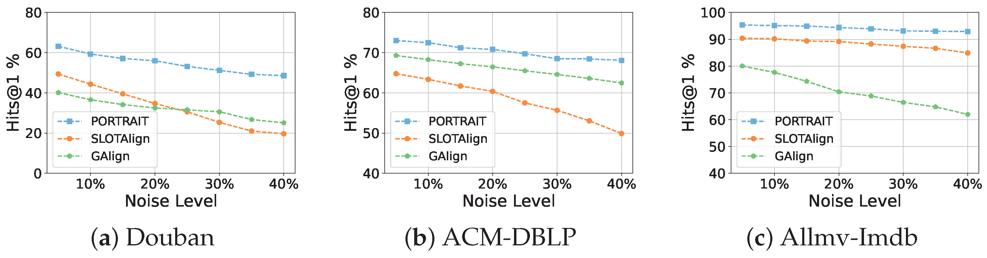
  • Robustness Analysis: To validate the robustness of our proposed model, we conduct comprehensive experiments involving edge perturbations (ranging from 10% to 40% noise ratios) across three real-world datasets. For comparative analysis, we selected two representative baseline methods: GAlign as the embedding-based approach, and SLOTAlign as the optimal transport-based method. As illustrated in Figure 6, our model demonstrates consistently superior robustness across all noise levels, exhibiting significantly smaller performance degradation compared to baseline methods. Particularly noteworthy is the observation that at 30% noise contamination, a substantial perturbation level, our model maintains prediction accuracy comparable to that achieved by competing methods under noise-free conditions.
  • Parameter Sensitivity: We study the effects of hyperparameters on model accuracy, including the number of layers K in the attribute propagation step, the ratio of the pseudo-anchors, and the temperature parameter in the SCP module on the two real datasets. We use Hits@1 as the evaluation metric. The results are presented in Figure 7. By analyzing the impact of attribute propagation layers, a subtle decline in performance on the Douban dataset is noticeable with the increasing value of K. We speculate that this decline may be attributed to a certain degree of oversmoothing, potentially caused by the heightened number of layers. Interestingly, as the pseudo-anchor ratio increases, the model’s performance initially improves, followed by a slight decline. We attribute this phenomenon to higher confidence (92%) in pseudo-anchors within a smaller range; as the ratio grows, additional noise is introduced, which diminishes performance. Meanwhile, we observe a slight improvement in performance on the ACM-DBLP dataset as the temperature coefficient increases. In general, our model exhibits consistent robustness to variations of hyperparameters, highlighting the stability of our proposed approach.
  • Efficiency Comparison: To evaluate the computational efficiency of our model, we measure the runtime to convergence across three datasets. As shown by Figure 8 and Figure 9, our framework achieves significantly faster convergence on real-world datasets compared to baseline methods. This advantage becomes particularly pronounced on larger-scale datasets (e.g., ACM-DBLP), which we attribute to the model’s enhanced expressive power, which enables faster convergence with fewer epochs, and the matrix multiplication in Gromov–Wasserstein learning process could fully leverage the computing power of GPUs. For the synthetic dataset PPI, all methods achieve comparable efficiency.

4.3. Properties of OT-Based Methods

To further validate our motivation, we conduct a more detailed analysis of the OT-based graph alignment process across different datasets, and investigate the correlation between node degrees and the row-wise (column-wise) maximum alignment probabilities. Table 5 shows the average values for top-10% to 30% and the remaining nodes as well as the entire node set. It is clear that a strong correlation exists between the degree of a node and the predicted alignment probability, leading to higher accuracy. Meanwhile, we show the relationship between node degree and prediction accuracy (i.e., Hits@1) during the learning process. For ACM-DBLP, Douban, and PPI, we demonstrate the results of GWL (Figure 10a–d, Figure 11a–d, and Figure 12a–d), SLOTAlign (Figure 10e–h, Figure 11e–h, and Figure 12e–h), and PORTRAIT (Figure 10i–l, Figure 11i–l, and Figure 12i–l), respectively. It is obvious that nodes of large degrees are first aligned. Moreover, as the time costs per epoch for different OT-based methods are close, we conclude that PORTRAIT converges much faster than the other two baselines (also see Figure 9).

5. Other Related Work

Existing works for graph alignment can be broadly categorized according to the problem inputs. Graph structure-based methods [7,15,19,20,41,42,43,44,45] only utilize topological information for alignment, while our model falls into the category of attributed graph alignment [3,9,12,14,33,39,46,47,48,49,50,51,52] where node attributes are also available. Another problem setting is knowledge graph (KG) alignment (e.g., [10,40,53]), and comprehensive surveys are referred to [54,55].
From the perspective of learning paradigm, consistency-based methods [9,12,56,57,58] are widely used for structure-only and attributed graph alignments. Embedding-based solutions [13,18,19,20,21] follow the idea of “Embed-Then-Cross-Compare” while GNNs are recently employed [17,40] and cross-graph propagation is considered [20]. Another line of work adopts adversarial learning [17,47]. Pei et al. [59] propose a curriculum learning approach, but they focus on the supervised setting with noise while we aim at OT-based methods without supervision. Similarly, [43] handles the degree differences in the embedding space of KG alignment for the semi-supervised setting. We also have witnessed a line of algorithms for efficient OT computation [60,61,62], which might accelerate graph alignment in the near future.

6. Conclusions and Limitation

We propose PORTRAIT, an unsupervised approach that enhances optimal transport-based graph alignment by leveraging attribute interactions and self-training. Specifically, we design flexible modules with enhanced expressive power to effectively integrate richer structural and attribute information, while introducing a cost normalization module to improve both accuracy and stability. Then, by selecting high-confidence matching nodes as pseudo-labels, we present a self-training strategy with our refined cost computation process to significantly enhance the accuracy of our model and other existing OT-based methods. Extensive experimental results demonstrate our model’s superior performance, achieving a 5% improvement in Hits@1, which effectively validates our motivations. Although the proposed method achieves outstanding prediction accuracy, scalability remains a challenge that will constitute the primary focus of our future research.

Author Contributions

Conceptualization, S.C.; Methodology, S.C.; Visualization, Z.Z. and M.X.; Writing—original draft, S.C.; Writing—review and editing, Y.L. All authors have read and agreed to the published version of the manuscript.

Funding

This research received no external funding.

Data Availability Statement

The datasets used in this paper can be obtained through the link https://github.com/SongyangChen2022/Dataset. The source code will be open-sourced after the paper review process.

Conflicts of Interest

The authors declare no conflicts of interest.

References

  1. Cao, X.; Yu, Y. Joint User Modeling Across Aligned Heterogeneous Sites Using Neural Networks. In Proceedings of the Machine Learning and Knowledge Discovery in Databases—European Conference, ECML PKDD 2017, Skopje, Republic of Macedonia, 18–22 September 2017. Part I. [Google Scholar]
  2. Farseev, A.; Nie, L.; Akbari, M.; Chua, T. Harvesting Multiple Sources for User Profile Learning: A Big Data Study. In Proceedings of the 5th ACM on International Conference on Multimedia Retrieval, Shanghai, China, 23–26 June 2015. [Google Scholar]
  3. Fey, M.; Lenssen, J.E.; Morris, C.; Masci, J.; Kriege, N.M. Deep graph matching consensus. arXiv 2020, arXiv:2001.09621. [Google Scholar]
  4. Feng, S.; Shen, D.; Nie, T.; Kou, Y.; Yu, G. A generation probability based percolation network alignment method. World Wide Web 2021, 24, 1511–1531. [Google Scholar] [CrossRef]
  5. Ni, J.; Tong, H.; Fan, W.; Zhang, X. Inside the atoms: Ranking on a network of networks. In Proceedings of the The 20th ACM SIGKDD International Conference on Knowledge Discovery and Data Mining, KDD ’14, New York, NY, USA, 24–27 August 2014. [Google Scholar]
  6. Kazemi, E.; Hassani, S.H.; Grossglauser, M.; Modarres, H.P. PROPER: Global protein interaction network alignment through percolation matching. BMC Bioinform. 2016, 17, 1–16. [Google Scholar] [CrossRef] [PubMed]
  7. Liu, Y.; Ding, H.; Chen, D.; Xu, J. Novel Geometric Approach for Global Alignment of PPI Networks. In Proceedings of the Thirty-First AAAI Conference on Artificial Intelligence, San Francisco, CA, USA, 4–9 February 2017. [Google Scholar]
  8. Tang, J.; Zhang, J.; Yao, L.; Li, J.; Zhang, L.; Su, Z. ArnetMiner: Extraction and mining of academic social networks. In Proceedings of the 14th ACM SIGKDD International Conference on Knowledge Discovery and Data Mining, Las Vegas, NV, USA, 24–27 August 2008. [Google Scholar]
  9. Zhang, S.; Tong, H.; Jin, L.; Xia, Y.; Guo, Y. Balancing Consistency and Disparity in Network Alignment. In Proceedings of the KDD ’21: The 27th ACM SIGKDD Conference on Knowledge Discovery and Data Mining, Singapore, 14–18 August 2021. [Google Scholar]
  10. Li, Y.; Chen, L.; Liu, C.; Zhou, R.; Li, J. Generative adversarial network for unsupervised multi-lingual knowledge graph entity alignment. World Wide Web 2023, 26, 2265–2290. [Google Scholar] [CrossRef]
  11. Shu, Y.; Zhang, J.; Huang, G.; Chi, C.H.; He, J. Entity alignment via graph neural networks: A component-level study. World Wide Web 2023, 26, 4069–4092. [Google Scholar] [CrossRef]
  12. Zeng, Z.; Zhang, S.; Xia, Y.; Tong, H. PARROT: Position-Aware Regularized Optimal Transport for Network Alignment. In Proceedings of the ACM Web Conference 2023, WWW 2023, Austin, TX, USA, 30 April–4 May 2023. [Google Scholar]
  13. Yan, Y.; Zhang, S.; Tong, H. BRIGHT: A Bridging Algorithm for Network Alignment. In Proceedings of the WWW ’21: The Web Conference 2021, Ljubljana, Slovenia, 19–23 April 2021; Leskovec, J., Grobelnik, M., Najork, M., Tang, J., Zia, L., Eds.; 2021. [Google Scholar]
  14. Tang, J.; Zhang, W.; Li, J.; Zhao, K.; Tsung, F.; Li, J. Robust Attributed Graph Alignment via Joint Structure Learning and Optimal Transport. In Proceedings of the 39th IEEE International Conference on Data Engineering, ICDE 2023, Anaheim, CA, USA, 3–7 April 2023. [Google Scholar]
  15. Xu, H.; Luo, D.; Zha, H.; Carin, L. Gromov-Wasserstein Learning for Graph Matching and Node Embedding. In Proceedings of the 36th International Conference on Machine Learning, ICML 2019, Long Beach, CA, USA, 9–15 June 2019; Chaudhuri, K., Salakhutdinov, R., Eds.; 2019. [Google Scholar]
  16. Wang, H.; Hu, R.; Zhang, Y.; Qin, L.; Wang, W.; Zhang, W. Neural Subgraph Counting with Wasserstein Estimator. In Proceedings of the SIGMOD ’22: International Conference on Management of Data, Philadelphia, PA, USA, 12–17 June 2022. [Google Scholar]
  17. Gao, J.; Huang, X.; Li, J. Unsupervised Graph Alignment with Wasserstein Distance Discriminator. In Proceedings of the KDD ’21: The 27th ACM SIGKDD Conference on Knowledge Discovery and Data Mining, Singapore, 14–18 August 2021. [Google Scholar]
  18. Yan, Y.; Liu, L.; Ban, Y.; Jing, B.; Tong, H. Dynamic Knowledge Graph Alignment. In Proceedings of the Thirty-Fifth AAAI Conference on Artificial Intelligence, AAAI 2021, Thirty-Third Conference on Innovative Applications of Artificial Intelligence, IAAI 2021, The Eleventh Symposium on Educational Advances in Artificial Intelligence, EAAI 2021, Virtual Event, 2–9 February 2021. [Google Scholar]
  19. Liu, L.; Cheung, W.K.; Li, X.; Liao, L. Aligning Users across Social Networks Using Network Embedding. In Proceedings of the Twenty-Fifth International Joint Conference on Artificial Intelligence, IJCAI 2016, New York, NY, USA, 9–15 July 2016. [Google Scholar]
  20. Chu, X.; Fan, X.; Yao, D.; Zhu, Z.; Huang, J.; Bi, J. Cross-Network Embedding for Multi-Network Alignment. In Proceedings of the World Wide Web Conference, WWW 2019, San Francisco, CA, USA, 13–17 May 2019. [Google Scholar]
  21. Zhang, S.; Tong, H.; Xia, Y.; Xiong, L.; Xu, J. NetTrans: Neural Cross-Network Transformation. In Proceedings of the KDD ’20: The 26th ACM SIGKDD Conference on Knowledge Discovery and Data Mining, San Diego, CA, USA, 23–27 August 2020. [Google Scholar]
  22. Trung, H.T.; Van Vinh, T.; Tam, N.T.; Yin, H.; Weidlich, M.; Hung, N.Q.V. Adaptive network alignment with unsupervised and multi-order convolutional networks. In Proceedings of the 2020 IEEE 36th International Conference on Data Engineering (ICDE), Dallas, TX, USA, 20–24 April 2020; pp. 85–96. [Google Scholar]
  23. Wang, C.; Jiang, P.; Zhang, X.; Wang, P.; Qin, T.; Guan, X. GTCAlign: Global Topology Consistency-based Graph Alignment. IEEE Trans. Knowl. Data Eng. 2023, 36, 2009–2025. [Google Scholar] [CrossRef]
  24. Arjovsky, M.; Chintala, S.; Bottou, L. Wasserstein Generative Adversarial Networks. In Proceedings of the 34th International Conference on Machine Learning, ICML 2017, Sydney, NSW, Australia, 6–11 August 2017. [Google Scholar]
  25. Cuturi, M. Sinkhorn Distances: Lightspeed Computation of Optimal Transport. In Proceedings of the Advances in Neural Information Processing Systems 26: 27th Annual Conference on Neural Information Processing Systems 2013, Lake Tahoe, NV, USA, 5–8 December 2013. [Google Scholar]
  26. Villani, C. Optimal Transport: Old and New; Springer: Berlin/Heidelberg, Germany, 2009; Volume 338. [Google Scholar]
  27. Mémoli, F. Gromov—Wasserstein distances and the metric approach to object matching. Found. Comput. Math. 2011, 11, 417–487. [Google Scholar] [CrossRef]
  28. Wu, F.; de Souza, A.H., Jr.; Zhang, T.; Fifty, C.; Yu, T.; Weinberger, K.Q. Simplifying Graph Convolutional Networks. In Proceedings of the 36th International Conference on Machine Learning, ICML, Long Beach, CA, USA, 9–15 June 2019. [Google Scholar]
  29. Maretic, H.P.; Gheche, M.E.; Chierchia, G.; Frossard, P. GOT: An Optimal Transport framework for Graph comparison. In Proceedings of the Advances in Neural Information Processing Systems 32: Annual Conference on Neural Information Processing Systems 2019, NeurIPS 2019, Vancouver, BC, Canada, 8–14 December 2019. [Google Scholar]
  30. Maretic, H.P.; Gheche, M.E.; Chierchia, G.; Frossard, P. fGOT: Graph Distances Based on Filters and Optimal Transport. In Proceedings of the Thirty-Sixth AAAI Conference on Artificial Intelligence, AAAI 2022, Thirty-Fourth Conference on Innovative Applications of Artificial Intelligence, IAAI 2022, The Twelveth Symposium on Educational Advances in Artificial Intelligence, EAAI, Virtual Event, 22 February–1 March 2022. [Google Scholar]
  31. Xie, Y.; Wang, X.; Wang, R.; Zha, H. A Fast Proximal Point Method for Computing Exact Wasserstein Distance. In Proceedings of the Thirty-Fifth Conference on Uncertainty in Artificial Intelligence, UAI 2019, Tel Aviv, Israel, 22–25 July 2019; Globerson, A., Silva, R., Eds.; [Google Scholar]
  32. Vayer, T.; Courty, N.; Tavenard, R.; Chapel, L.; Flamary, R. Optimal Transport for structured data with application on graphs. In Proceedings of the 36th International Conference on Machine Learning, ICML 2019, Long Beach, CA, USA, 9–15 June 2019. [Google Scholar]
  33. Zhang, S.; Tong, H. FINAL: Fast Attributed Network Alignment. In Proceedings of the 22nd ACM SIGKDD International Conference on Knowledge Discovery and Data Mining, San Francisco, CA, USA, 13–17 August 2016. [Google Scholar]
  34. Page, L.; Brin, S.; Motwani, R.; Winograd, T. The Pagerank Citation Ranking: Bring Order to the Web; Technical Report; Stanford University: Stanford, CA, USA, 1998. [Google Scholar]
  35. Peyré, G.; Cuturi, M. Computational optimal transport: With applications to data science. Found. Trends® Mach. Learn. 2019, 11, 355–607. [Google Scholar] [CrossRef]
  36. Bolte, J.; Sabach, S.; Teboulle, M. Proximal alternating linearized minimization for nonconvex and nonsmooth problems. Math. Program. 2014, 146, 459–494. [Google Scholar] [CrossRef]
  37. Zhang, S.; Tong, H. Attributed Network Alignment: Problem Definitions and Fast Solutions. IEEE Trans. Knowl. Data Eng. 2019, 31, 1680–1692. [Google Scholar] [CrossRef]
  38. Zitnik, M.; Leskovec, J. Predicting multicellular function through multi-layer tissue networks. Bioinformatics 2017, 33, i190–i198. [Google Scholar] [CrossRef] [PubMed]
  39. Heimann, M.; Shen, H.; Safavi, T.; Koutra, D. REGAL: Representation Learning-based Graph Alignment. In Proceedings of the 27th ACM International Conference on Information and Knowledge Management, CIKM 2018, Torino, Italy, 22–26 October 2018. [Google Scholar]
  40. Wang, Z.; Lv, Q.; Lan, X.; Zhang, Y. Cross-lingual Knowledge Graph Alignment via Graph Convolutional Networks. In Proceedings of the 2018 Conference on Empirical Methods in Natural Language Processing, Brussels, Belgium, 31 October–4 November 2018. [Google Scholar]
  41. Chen, M.; Tian, Y.; Yang, M.; Zaniolo, C. Multilingual Knowledge Graph Embeddings for Cross-lingual Knowledge Alignment. In Proceedings of the Twenty-Sixth International Joint Conference on Artificial Intelligence, IJCAI 2017, Melbourne, Australia, 19–25 August 2017. [Google Scholar]
  42. Nassar, H.; Veldt, N.; Mohammadi, S.; Grama, A.; Gleich, D.F. Low Rank Spectral Network Alignment. In Proceedings of the 2018 World Wide Web Conference on World Wide Web, WWW 2018, Lyon, France, 23–27 April 2018. [Google Scholar]
  43. Pei, S.; Yu, L.; Hoehndorf, R.; Zhang, X. Semi-Supervised Entity Alignment via Knowledge Graph Embedding with Awareness of Degree Difference. In Proceedings of the World Wide Web Conference, WWW 2019, San Francisco, CA, USA, 13–17 May 2019. [Google Scholar]
  44. Pei, S.; Yu, L.; Zhang, X. Improving Cross-lingual Entity Alignment via Optimal Transport. In Proceedings of the Twenty-Eighth International Joint Conference on Artificial Intelligence, IJCAI 2019, Macao, China, 10–16 August 2019. [Google Scholar]
  45. Zhang, S.; Tong, H.; Maciejewski, R.; Eliassi-Rad, T. Multilevel network alignment. In Proceedings of the World Wide Web Conference, San Francisco, CA, USA, 13–17 May 2019; pp. 2344–2354. [Google Scholar]
  46. Chen, M.; Tian, Y.; Chang, K.; Skiena, S.; Zaniolo, C. Co-training Embeddings of Knowledge Graphs and Entity Descriptions for Cross-lingual Entity Alignment. In Proceedings of the Twenty-Seventh International Joint Conference on Artificial Intelligence, IJCAI 2018, Stockholm, Sweden, 13–19 July 2018. [Google Scholar]
  47. Li, C.; Wang, S.; Wang, H.; Liang, Y.; Yu, P.S.; Li, Z.; Wang, W. Partially Shared Adversarial Learning For Semi-supervised Multi-platform User Identity Linkage. In Proceedings of the 28th ACM International Conference on Information and Knowledge Management, CIKM 2019, Beijing, China, 3–7 November 2019. [Google Scholar]
  48. Su, S.; Sun, L.; Zhang, Z.; Li, G.; Qu, J. MASTER: Across Multiple social networks, integrate Attribute and STructure Embedding for Reconciliation. In Proceedings of the Twenty-Seventh International Joint Conference on Artificial Intelligence, IJCAI 2018, Stockholm, Sweden, 13–19 July 2018. [Google Scholar]
  49. Sun, Z.; Hu, W.; Li, C. Cross-Lingual Entity Alignment via Joint Attribute-Preserving Embedding. In Proceedings of the The Semantic Web-ISWC 2017-6th International Semantic Web Conference, Vienna, Austria, 21–25 October 2017. Part I. [Google Scholar]
  50. Yasar, A.; Çatalyürek, Ü.V. An Iterative Global Structure-Assisted Labeled Network Aligner. In Proceedings of the 24th ACM SIGKDD International Conference on Knowledge Discovery & Data Mining, KDD 2018, London, UK, 19–23 August 2018. [Google Scholar]
  51. Chen, S.; Lin, Y.; Liu, Y.; Ouyang, Y.; Guo, Z.; Zou, L. Enhancing robust semi-supervised graph alignment via adaptive optimal transport. World Wide Web 2025, 28, 22. [Google Scholar] [CrossRef]
  52. Chen, S.; Liu, Y.; Zou, L.; Wang, Z.; Lin, Y.; Chen, Y.; Pan, A. Combining Optimal Transport and Embedding-Based Approaches for More Expressiveness in Unsupervised Graph Alignment. arXiv 2024, arXiv:2406.13216. [Google Scholar]
  53. Sun, Z.; Hu, W.; Zhang, Q.; Qu, Y. Bootstrapping Entity Alignment with Knowledge Graph Embedding. In Proceedings of the Twenty-Seventh International Joint Conference on Artificial Intelligence, IJCAI 2018, Stockholm, Sweden, 13–19 July 2018. [Google Scholar]
  54. Zeng, W.; Zhao, X.; Tan, Z.; Tang, J.; Cheng, X. Matching Knowledge Graphs in Entity Embedding Spaces: An Experimental Study. IEEE Trans. Knowl. Data Eng. 2023, 35, 12770–12784. [Google Scholar] [CrossRef]
  55. Zeng, K.; Li, C.; Hou, L.; Li, J.; Feng, L. A comprehensive survey of entity alignment for knowledge graphs. AI Open 2021, 2, 1–13. [Google Scholar] [CrossRef]
  56. Koutra, D.; Tong, H.; Lubensky, D.M. BIG-ALIGN: Fast Bipartite Graph Alignment. In Proceedings of the 2013 IEEE 13th International Conference on Data Mining, Dallas, TX, USA, 7–10 December 2013. [Google Scholar]
  57. Zhan, Q.; Zhang, J.; Yu, P.S. Integrated anchor and social link predictions across multiple social networks. Knowl. Inf. Syst. 2019, 60, 303–326. [Google Scholar] [CrossRef]
  58. Singh, R.; Xu, J.; Berger, B. Global alignment of multiple protein interaction networks with application to functional orthology detection. Proc. Natl. Acad. Sci. USA 2008, 105, 12763–12768. [Google Scholar] [CrossRef] [PubMed]
  59. Pei, S.; Yu, L.; Yu, G.; Zhang, X. Graph Alignment with Noisy Supervision. In Proceedings of the WWW ’22: The ACM Web Conference 2022, Lyon, France, 25–29 April 2022. [Google Scholar]
  60. Li, M.; Yu, J.; Li, T.; Meng, C. Importance Sparsification for Sinkhorn Algorithm. CoRR 2023. [Google Scholar] [CrossRef]
  61. Li, M.; Yu, J.; Xu, H.; Meng, C. Efficient Approximation of Gromov-Wasserstein Distance using Importance Sparsification. CoRR 2022. [Google Scholar] [CrossRef]
  62. Klicpera, J.; Lienen, M.; Günnemann, S. Scalable Optimal Transport in High Dimensions for Graph Distances, Embedding Alignment, and More. In Proceedings of the 38th International Conference on Machine Learning, ICML 2021, Virtual Event, 18–24 July 2021; Meila, M., Zhang, T., Eds.; [Google Scholar]
Figure 1. Overview of our approach.
Mathematics 13 01971 g001
Figure 2. Illustration of attribute propagation and interaction.
Mathematics 13 01971 g002
Figure 3. Illustration of the unsupervised GW learning phase.
Mathematics 13 01971 g003
Figure 4. Illustration of the self-training phase.
Mathematics 13 01971 g004
Figure 5. Number of nodes correctly aligned and corresponding accuracy (Hits@1) per degree.
Mathematics 13 01971 g005
Figure 6. Robustness analysis in noisy conditions.
Mathematics 13 01971 g006
Figure 7. Impact of attribute propagation layers and temperature parameter of SCP.
Mathematics 13 01971 g007
Figure 8. Convergence curve of PORTRAIT.
Mathematics 13 01971 g008
Figure 9. Efficiency comparison of different models on three datasets.
Mathematics 13 01971 g009
Figure 10. Accuracy vs. degree varying #epoch on ACM-DBLP for GWL, SLOTAlign, and PORTRAIT.
Mathematics 13 01971 g010
Figure 11. Accuracy vs. degree varying #epoch on Douban for GWL, SLOTAlign, and Opt-SIGMA.
Mathematics 13 01971 g011
Figure 12. Accuracy vs. degree varying #epoch on PPI for GWL, SLOTAlign, and PORTRAIT.
Mathematics 13 01971 g012
Table 1. Table of notations.
NotationDescription
G s , G t The two attributed graphs to be aligned
A s , A t The adjacency matrices of G s and G t
X s , X t The node attributes
n 1 , n 2 The number of nodes in G s and G t ( n 1 n 2 )
C s , C t The intra-graph cost matrices for G s and G t
C g w d , C i n t The inter-graph cost matrix (of size n 1 × n 2 )
T The alignment matrix
Table 2. Datasets and their statistics.
Dataset n = | V | m = | E | FeaturesAnswers
Douban [33]111830225381118
3906 16,328
ACM-DBLP [37]9872 39,561 176325
9916 44,808
PPI [38]1767 16,159 501767
1767 16,159
Allmv-Imdb [22]5713 119,073 145174
6011 124,709
Table 3. Evaluation of the model accuracy. We mark the best and second-best results of all unsupervised model variants with bold font and underline, respectively.
Douban Online–OfflineACM-DBLPPPIAllmv-Imdb
ModelHits@1Hits@5Hits@10Hits@1Hits@5Hits@10Hits@1Hits@5Hits@10Hits@1Hits@5Hits@10
WAlign39.4562.2571.4763.4383.1886.5888.5192.9893.8752.5970.9476.53
GAlign45.2467.7778.1370.1786.9891.2589.0790.2894.0482.1486.3590.03
GTCAlign60.9176.7782.1860.8375.5280.1189.2592.8194.0784.7389.9291.37
GWL3.498.329.9356.3677.0982.1886.7688.0688.6287.8292.3193.83
GWL + ST10.5523.6130.5964.1885.3189.6989.2493.0993.9990.1293.5394.07
SLOTAlign51.4373.4377.7365.6385.8487.7689.3092.5393.4990.6092.7593.12
SLOTAlign + ST55.1878.0382.8669.8888.6291.2889.3693.0194.0392.0793.8194.26
PORTRAIT63.3286.4090.8773.4590.1393.5089.7593.0494.1795.3396.2796.72
PORTRAIT w/o ST58.6878.3583.5469.0587.0490.6189.3692.6493.6693.7594.7995.26
PORTRAIT w/o ST+ Θ 50.4568.2572.9066.2284.9687.3289.2592.3093.0689.9893.0193.79
PORTRAIT w/o ST+Norm45.6163.9568.9263.5481.1484.6285.7489.5990.7287.9692.7793.91
Table 4. Evaluation of our self-training strategy.
Douban Online–OfflineACM-DBLPPPIAllmv-Imdb
ModelHits@1Hits@5Hits@10Hits@1Hits@5Hits@10Hits@1Hits@5Hits@10Hits@1Hits@5Hits@10
PORTRAIT63.4286.4090.8773.4590.1393.5089.7593.0494.1795.3396.2796.72
PORTRAIT w/degree-based62.2586.2590.7872.6689.6693.3589.5893.0394.1395.1296.1896.39
PORTRAIT w/PARROT58.3281.9286.3570.6889.1692.8889.6092.9294.1194.3395.2995.61
[1] PORTRAIT includes the self-training phase.
Table 5. Correlation between node degree and max k T ( i , k ) (resp. max i T ( i , k ) ).
Douban Online–OfflineACM-DBLP
Set of Nodes G s G t G s G t
Top 10% 2.26 × 10 4 2.36 × 10 4 8.63 × 10 5 8.23 × 10 5
Top 30% 1.94 × 10 4 1.94 × 10 4 7.79 × 10 5 7.83 × 10 5
All 1.28 × 10 4 1.11 × 10 4 6.38 × 10 5 6.39 × 10 5
Last 70% 9.97 × 10 5 7.61 × 10 5 5.77 × 10 5 5.77 × 10 5
Disclaimer/Publisher’s Note: The statements, opinions and data contained in all publications are solely those of the individual author(s) and contributor(s) and not of MDPI and/or the editor(s). MDPI and/or the editor(s) disclaim responsibility for any injury to people or property resulting from any ideas, methods, instructions or products referred to in the content.

