Abstract
Visceral leishmaniasis (VL), a chronic disease caused by Leishmania infantum, is more prevalent in males than females. Control strategies that do not take this disparity into account can be suboptimal. We extended a sex-structured VL model by introducing four control variables: insecticide-treated bed nets, vector control, medical treatment, and animal culling. The study evaluates six intervention strategies and calculates the incremental cost-effectiveness ratio to assess their impact on disease transmission and cost-effectiveness. The analysis shows that, without interventions, the disease remains endemic with significant health and socioeconomic consequences. The proposed strategy, which applies all four controls, emerges as the most effective and cost-efficient strategy, leading to an exponential reduction in disease prevalence across human, vector, and animal populations. Strategies without animal culling and vector control followed in effectiveness. Moreover, it was found that applying up to 50% of the controls to females, compared to males, can still eliminate VL within the planning period.
Keywords:
sex-structured VL model; vector-borne disease; optimal control; disease control strategies; cost-effectiveness analysis MSC:
92C60; 34D20; 93C15; 49M05; 34H05
1. Introduction
A chronic infectious disease caused by Leishmania infantum, visceral leishmaniasis (VL), also referred to as kala-azar, is the second-largest parasitic killer in the world (after malaria) [1,2]. An estimated 12 million individuals are affected by the disease worldwide in 98 endemic countries, and an additional 350 million are at risk of contracting it [3]. The vector-borne disease, VL, is transmitted through the bite of a very small flying insect, the female adult sandfly. Warm and humid weather is suitable for sandflies to flourish in [4]. Different interventions have been implemented in various endemic areas of the world to control the transmission of VL. These include personal protection through the use of clothes that cover as much of the body as possible, avoiding being outside between dusk and dawn, utilizing insecticide-treated bed nets, use of indoor and outdoor spraying of insecticides, and using window and door screens to prevent sandflies bites [5,6], together with WHO-recommended therapies such as liposomal amphotericin B, Miltefosine, Pentavalent antimonials, and Paromomycin [7]. However, due to the costs of medicines and the administration route, locating effective VL control strategies continues to be challenging
These models are indispensable tools for understanding, predicting, and controlling the spread of infectious diseases. They provide critical insights that inform policy decisions, optimize resource allocation, support emergency response efforts, and drive innovation in disease control strategies. Hence, numerous modeling studies of VL have been conducted to understand the impact of different intervention strategies and to describe and predict how the disease spreads (see [8,9,10,11,12,13,14,15,16] and the reference therein); while the mathematical models of VL are valuable for understanding the disease dynamics, they do not explicitly optimize control strategies. Optimal control models provide more rigorous and efficient tools for designing and implementing effective disease control strategies. However, some studies have been conducted to investigate the optimal control strategies for controlling the spread of VL.
For example, Pantha et al. [17] developed a mathematical model for VL transmission dynamics involving human, canine, and vector populations. The goal was to identify effective control measures for reducing VL burden and guiding public health interventions in endemic areas. They evaluated three control measures using optimal control theory: personal protection, insecticide spraying, and culling infected canine reservoirs. The simulation results showed that combining these interventions could eliminate VL from the region. Zhao et al. [18] developed a mathematical model for zoonotic visceral leishmaniasis (ZVL) in Brazil using a modified SEIR-type approach, focusing on dogs as reservoirs. They classified the dog population into susceptible, exposed, infected, and recovered categories and the human and sandfly populations into similar compartments. Mathematical analysis indicated the possibility of backward bifurcation. They introduced three time-dependent controls using optimal control theory: dog vaccination, sandfly control with insecticides, and personal human protection. Numerical simulations showed that vector control via insecticide spraying was the most effective strategy, while culling dogs was ineffective. However, the study lacked validation with real data and did not include a cost-effectiveness analysis.
Ghosh et al. [19] developed a compartmental VL model considering human, animal, sandfly, and non-adult sandfly populations. The human population was divided into six classes, including asymptomatic, symptomatic, and post-kala-azar dermal leishmaniasis (PKDL)-infected individuals. Global sensitivity analysis identified key parameters affecting the cost function, and the model was validated with 2013 weekly VL incidence data from South Sudan. The model used three time-dependent controls: treatment of infected individuals, non-adult-stage vector control, and adult-stage vector control. Cost-effectiveness analysis showed that combining treatment and non-adult-stage vector control was the most cost-effective strategy. Augusto et al. [20] developed a deterministic model for malaria–VL co-infection to understand its dynamics and find cost-effective control strategies. Using the basic model by ELmojtaba [9], they introduced four time-dependent controls: personal human protection, insecticide-treated bed nets, culling of infected reservoir animals, and insecticides. Their results show that combining personal protection, indoor residual spraying, and reservoir culling is the most cost-effective approach for controlling malaria–VL co-infection. In several endemic regions of the world, the results of numerous studies have demonstrated that males are more severely impacted by VL than females. The observed sex disparity in visceral leishmaniasis is likely influenced by a combination of behavioral, biological, socioeconomic, and environmental factors. Conducting a sex-structured disease dynamics model for visceral leishmaniasis allows for a more comprehensive understanding of transmission dynamics. To address this issue, a sex-structured VL disease transmission model was conducted by Awoke et al. [21]. However, the research work did not include optimal control and cost-effectiveness analysis. The optimal control plays a crucial role in disease dynamics models. It offers insightful information about the possible effects of various intervention strategies (e.g., insecticide-treated bed nets, vector control, and medical treatment), and supports long-term planning goals by taking the sustainability and feasibility of intervention strategies over extended time horizons into account. Furthermore, it helps public health decision makers to prioritize disease control strategies during resource allocation and maximizes the use of limited resources (for example vaccines, drugs, and medical staff). Since VL treatments are very expensive, it is very important to study sex-structured VL models that incorporate disease control mechanisms and propose cost-effective intervention strategies.
Managing VL poses a financial burden on local communities in countries where the disease is prevalent, perpetuating a cycle of illness and poverty. Strategic allocation of public funds towards control programs could alleviate this burden by reducing the prevalence of VL [22]. To this end, employing dynamic models that incorporate an optimal control theory is essential for assessing intervention strategies and devising an economically efficient policy to contain the disease. The motivation for this research arises from the considerable public health challenge posed by VL, a disease that predominantly affects males; while many VL models, including those incorporating animal reservoirs and optimal control strategies, have been studied, there remains a gap in analyzing the cost-effectiveness of interventions in sex-structured populations. Building on the VL model developed by Awoke et al. [21], this article introduces four time-dependent control interventions: the use of insecticide-treated bed nets, vector control through residual spraying and environmental management, medical treatment, and infected animal culling. To the best of the knowledge of the authors, no study has yet explored the cost-effectiveness of such a comprehensive, sex-structured approach to VL control. To evaluate whether sex differences influence optimal control strategies, we incorporated parameters for the use of insecticide-treated bed nets and medical treatment. By addressing this gap, this research will provide crucial insights that can directly benefit both local communities and policymakers. A thorough cost-effectiveness analysis will identify the most cost-effective strategies for reducing VL transmission, helping to optimize limited resources in low-income regions where the disease is prevalent. This research will also equip policymakers with evidence-based recommendations, allowing them to prioritize interventions that offer the greatest health benefits for the lowest cost, ultimately contributing to more sustainable and effective public health strategies. Hence, our study aims to integrate effective preventive and control measures for visceral leishmaniasis (VL) into the existing sex-structured model. We intend to assess the cost-effectiveness of these interventions and propose an optimal control strategy to enhance decision-making processes.
The rest of the manuscript is organized as follows: Section 2, presents the model formulation, control strategies and analysis of key properties, including positivity, boundedness, and the basic reproduction number with controls. This sections also introduces the optimal control problem and its characterization. Section 3 presents the results and discussion. Conclusions are given in Section 4.
2. Methods
Controlling VL remains challenging in different endemic areas of the world for different reasons, such as the complexity of the transmission, lack of effective vaccine, cost of treatment, and socioeconomic factors. In addition, the disease mainly affects the male human population. Hence, there is a need to develop comprehensive cost-effective control strategies that will address these challenges. By optimizing control measures across different sex groups and considering trade-offs between intervention options, optimal control helps maximize the impact of interventions and improve disease control efforts. The most powerful VL disease transmission control mechanisms are the use of insecticide-treated bed nets and medical treatment of infected humans together with vector control strategies. In this work, we want to consider these interventions as time-dependent control functions and incorporate them into the sex-structured VL model proposed in [21]. The total human population is initially divided into male and female sub-populations, with each further classified into five compartments: susceptible males and females (, ), exposed males and females (, ), asymptomatic males and females (, ), actively infected males and females (, ), and recovered males and females (, ). The sandfly population is split into susceptible () and infected () groups, while the reservoir population is categorized into susceptible (), infected (), and recovered () groups. The description of the model parameters are indicated in Table 1; for detail, please refer to [21].

Table 1.
Definition of model parameters.
As described in [23,24], the possible interventions for visceral leishmaniasis can be categorized as follows: applying preventive mechanisms through the use of insecticide-treated bed nets (ITNs), vector control with the use of insecticides, treatment of infected individuals, and animal culling. The practical applications of these mechanisms and the assumptions used in this work are described below.
- 1.
- Preventive mechanisms through the use of ITNs.The WHO-recommended VL preventive strategies include the use of insecticide-treated sandfly nets [25]. In order to curb the spread of VL, in a study by [26], a breakthrough in reducing the spread of VL was achieved after the introduction of ITNs. Due to its practical applicability, we are considering the use of ITNs as one of the control strategies. Using ITNs reduces the probability of humans being bitten. Furthermore, since the nets are treated with insecticides, they kill vectors. Therefore, we used the following two assumptions formulated in [20,27].
- (a)
- The mathematical expression for the use of ITNs in reducing the human–vector contact rate is described by the following relation:where and are the maximum and minimum possible number of bites a host population receives per week, respectively. Since most sandfly biting activity occurs during the early evening before most people go to sleep, and due to other limitations in the use of INTs, the maximum control effort is assumed to be . Hence, . Applying different interventions, such as insecticide-treated bed nets and medication, to different sexes (male and female human populations) in the control of VL might raise ethical considerations. Males and females often have different exposure risks to sandflies. In VL-endemic areas, males may work outdoors in high-risk settings where they are more exposed to sandfly bites, while females may spend more time indoors. Tailoring interventions to these behavioral patterns, such as providing stronger protection for males who are more exposed outdoors, may be a targeted and effective strategy for disease control. In addition to these, the availability of limited resources in public health programs often necessitates prioritizing interventions for populations at greater risk. Since the data reveal that men are at higher risk of contracting the disease than women, focusing certain interventions like availing treated bed nets or medications on that group can maximize the impact of disease control efforts. Due to these reasons, we assumed that the intervention rates for females are reduced by a proportion of for the use of bed nets and by for the use of medical treatment as compared to that of their male counterparts, where . In this work, the expression for the use of ITNs is based on the concept formulated in Asfaw et al. [27]. Therefore, the forces of infection for the male human population (), female human population (), and vector population () are re-written as follows:where . Our model is based on the assumption that vector bites are distributed in fixed proportions among males, females, and reservoir hosts. However, in real-world scenarios, the use of bed nets by a subset of the human population could alter this distribution. Specifically, when some individuals are protected by bed nets, vectors may shift their biting behavior toward unprotected groups, potentially leading to increased exposure among unprotected groups such as reservoir hosts. We acknowledge that this adaptive biting behavior is not captured in our current model.
- (b)
- Since bed nets are treated with insecticides, they have the capacity to kill vectors that land on the net. Hence, if the natural death rate of vectors is , ITNs usage increases the sandfly death rate by . This is mathematically represented bywhere represents the capability of insecticide-treated bed nets to kill sandflies and represents the death rate of adult sandflies due to insecticide-treated bed nets.
- 2.
- Vector control: The incidence rate of VL is increasing in some endemic regions of the world, including Kenya, Ethiopia, and Sudan [28], as a result of the serious side effects of current VL medications and the lack of an effective vaccination. Programs to eradicate leishmaniasis, therefore, mainly rely on vector control using insecticides and environmental management. The goal of environmental management is to eliminate or make places undesirable for sandflies to nest and rest, as well as to kill the pre-adult stage of vectors. Tree stump clearance, soil and crack filling, the routine cleaning of the per-domicile area and animal shelters, and trash removal are common vector control methods in environmental management [29]. Additionally, the most effective method of controlling sandflies is the use of chemical interventions such as indoor residual spraying (IRS), which is associated with a decrease in the lifespan of sandflies, leading to a subsequent decline in their population [12,30,31]. By reducing the lifespan of sandflies, the vector is less likely to survive long enough to acquire infection and to infect a host again. As the death rate of vectors increases, they spend less time in an infected state. Taking this into account, we incorporate a time-dependent control that represents an additional vector control effort through the use of environmental management and indoor residual spraying into the VL model. If the current natural mortality rate of vectors is , then the number of additional deaths of non-adult sandflies after the use of vector control interventions will be , where represents the effectiveness of insecticide spraying in killing sandflies. This implies that of Equation (4) will be updated by an additional term, , such thatFurthermore, the recruitment rate of vectors () will decrease by , as the application of insecticides is expected to destroy the breeding sites and kills the non-adult-stage sandflies. Hence, is updated by , where . Note here that and must satisfy the condition that
- 3.
- Treating infected individuals: Treatment is an important method to recover from the disease. Treatment has an effective role in preventing and controlling the spreading of the disease. Proper and timely treatment can reduce the total prevalence of the disease. However, treatment alone will not be enough to truly halt the transmission of VL [32,33]. The efficacy of VL drugs varies from one endemic area to another. We assume that the efficacy of VL drug is . If and are the recovery rates of male and female human host, then the mathematical expression for the formulation of controls with an additional treatment effort () is given by: and . Where represents the natural recovery rate of the male human host, represents the natural recovery of female human hosts, and is a modification parameter, as stated before, with for every time .
- 4.
- Culling infected animals: Dogs are the most important reservoirs of VL infection in domestic settings, while other animals can serve as a source of VL infection [24]. As a result, it is believed that having infected dogs increases the risk of VL in people in endemic areas. Culling leishmania-seropositive reservoirs such as dogs has been recommended as a control measure in many VL endemic countries [34]. It is indicated in [17,20] that the culling of infected animals is a cost-effective VL control strategy, together with other interventions. Hence, we consider the culling of infected dogs as a control strategy. Given and , which represent the natural and disease-induced mortality rates of infected dogs, provides the mathematical expression for the rate at which infected dogs diminish as a result of further culling effort , where for every time .
In general, by considering all these, we incorporate the above four VL intervention strategies in the VL model formulated and analyzed in [21]. Since most governments cannot implement intervention programs indefinitely, we considered the optimal control problem with a fixed terminal time , where T is the final time. The corresponding system of differential equations, based on the schematic diagram in Figure 1, can be written as in Equation (6) once these control parameters have been applied to the model system.
where and . with , , and are as indicated in Equations (2) and (3). , , , and . The model system (6) is appended with initial conditions:
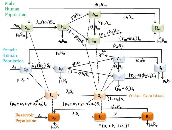
Figure 1.
Schematic diagram for VL compartmental model in which the human population is classified based on their sex.
2.1. Model Analysis
2.1.1. Boundedness and Positivity of Solutions with Constant Control Parameters
For the VL model system (6) to be epidemiologically meaningful, it is important to determine that all its state variables are non-negative for all time and that the region defined in Theorem 1 is positively invariant.
Theorem 1.
Proof.
The proof of Theorem 1 proceeds in a similar manner to the proof of Theorem 1 by Awoke et al. [21]. For brevity, we omit the details here, as they follow similar reasoning and steps as those presented in [21]. □
2.1.2. Disease-Free Equilibrium Point (DFE)
The model system (6) has a disease-free equilibrium (DFE) given by
2.1.3. Basic Reproduction Number with Constant Controls
As indicated in [35], the basic reproduction number () is defined as the average number of secondary infections that occur when one infective is introduced into a completely susceptible host population.
We calculate the basic reproduction number, , of the model system (6) using the next generation matrix approach proposed by [35]. To apply this method, we define as the column–vector of the rates of the appearance of new infections in each compartment; is the column–vector of the rates of transfer of individuals into the particular compartment; and is the column–vector of the rates of transfer of individuals out of the particular compartment. Then, for each compartment, where . Considering the system (6) has eight infected classes, namely , and , we obtain
Similarly, the Jacobian of (10) with respect to , and at gives
where ,, , , , , .
The basic reproduction number () is then given by the spectral radius of the next generation matrix, , and it is found to be
where
Remark 1.
The formula for basic reproduction number with control has three parts and is epidemiologically interpreted as follows:
- 1.
- The quantity is associated with the contribution of infected reservoirs;
- 2.
- The quantity is associated with the contribution of infected male humans;
- 3.
- The quantity is associated with the contribution of infected female humans in the spread of the disease at its initial stage.
Theorem 2.
The disease-free equilibrium (DFE) of the model system (6) with control is locally asymptotically stable whenever and unstable if .
Proof.
This is an immediate consequence of Theorem 2 in [35]. □
The epidemiological implication of Theorem 2 is that VL can be effectively controlled in the host and reservoir populations (humans and animal reservoirs) if the initial numbers of infected humans, reservoirs, and vectors are small enough (i.e., in the basin of attraction of the non-trivial disease-free equilibrium, ).
To understand how modifications in controls influence the basic reproduction number (), we perform partial differentiation of with respect to each control (, , , and ), by keeping the other parameters as a constant:
where
The rate of change of with respect to each control (,, , and ) is negative. This shows that increasing the values of the controls decreases the value of the basic reproduction number (). Therefore, employing ITNs for male and female human populations, medical treatment for infected male and infected female human populations, vector control, and removing infected animals will decrease the average number of new infections and, hence, the prevalence of the disease.
We can observe from Figure 2 that the use of additional effective medical treatment decreases the disease’s prevalence.
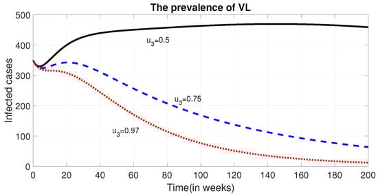
Figure 2.
Effect of treatment of infected humans () on the prevalence of VL. The figure illustrates how varying levels of the control variable (), representing treatment efforts for infected individuals, influence the overall prevalence of visceral leishmaniasis (VL) in the human population over time.
Remark 2.
The global stability analysis, parameter estimation, model calibration, and uncertainty analysis of the sex-structured VL model under constant control strategies were comprehensively addressed in a previous study [21]. The current research builds upon and extends that foundational work by introducing time-dependent control interventions to better capture the dynamics and effectiveness of varying control measures over time. To maintain focus and avoid redundancy, the detailed mathematical analyses previously conducted, such as the stability and uncertainty analyses, are not repeated in this paper. Interested readers are encouraged to consult Awoke et al. [21] for a thorough discussion of these aspects.
2.2. Optimal Control
2.2.1. Definition of Cost Function
We want to find the controls that minimize the total number of infected human populations and the cost of controls. This implies that finding optimal values of , , , and that minimize the cost function , where
Which is subject to the differential Equation (6), where T is the final time; the constants , , , , , , , , , and are values that will balance the units of measurement and may indicate the importance of one type of intervention over the other. and represent the cost on the population of actively infected male and female individuals as well as and represent the cost on the population of asymptomatically infected male and female individuals. Moreover, the terms and represent the individual treatment costs of male and female human host that receive treatment, respectively; represents the cost of implementing the control on ITNs, represents the cost of vector control, represents community-level treatment costs related to the preparation and facility setup for treatment, and represents the cost of removing infected reservoir animals; while the quadratic form of the cost function is mathematically advantageous, it also has practical biological and economic significance. The quadratic dependence on control efforts reflects the fact that, as the intensity of interventions increases, costs tend to rise disproportionately. Several factors contribute to this phenomenon. For example, initial interventions, such as moderate dog culling or bed net distribution, might be relatively affordable. However, achieving broader coverage often requires significantly more resources, leading to higher logistical and operational expenses. Additionally, while culling a small number of infected reservoir animals may be manageable, scaling up this effort could encounter increased community resistance, further elevating costs. The quadratic formulation of control costs is widely used in objective functions of optimal control problems, offering a familiar and well-understood approach within the field. We seek to find optimal controls , , , and , such that
where the admissible set
Considering the objective function in (12), we have the optimal control problem:
subject to the system in Equation (6) and bounded controls.
2.2.2. Existence and Characterization of Optimal Control Solution
Examining the conditions that can assure the existence of a solution to our optimum control issue will be the first step. The following theorem shows the existence of the optimal control solution to the above optimal control problem [36,37].
Theorem 3.
Proof.
The non-trivial requirements on the set of admissible controls and on the set of end conditions are verified from Fleming and Rishel’s theorem [36].
- A.
- The set of all solutions to the system (6) with corresponding control functions in is non-empty.
- B.
- The state system can be written as a linear function of the control variables with coefficients dependent on time and the state variables.
- C.
- The integrand L in (12) from objective functional with is convex on and satisfies where and .In order to establish condition A, we refer to Picard–Lindelöf’s theorem from [38]. If the solutions to the state equations are bounded, and the state equations are continuous and Lipschitz with respect to the state variables, then there exists a unique solution to the system for every admissible control . The total male human population is bounded between and , while the female human, reservoir, and sandfly populations are bounded above , , and , respectively, with lower bounds , , and . With these bounds, the state system is continuous, bounded, and Lipschitz with respect to the state variables, proving condition A holds. Condition B is verified by observing the linear dependence of the state equations on controls , , and . Finally, to verify condition C by definition from [39,40] any constant, linear and quadratic functions are convex. So , ,, and are convex on . Since linear combination of convex functions are also convex, the integrand is convex on .To prove the bound on the L, we adopted the method in [41]. We note that, by the definition of , we have
□
2.2.3. Characterization of Optimal Control Solution
To formulate the necessary conditions for optimality, we need to define the Hamiltonian function of the optimal control problem (14). The Hamiltonian equation with marginal cost function, state variables, and adjoint variables is given by
where is a function as defined before in Equation (6). By using Pontryagin’s Maximum Principle [36], we derive the necessary conditions for the optimal controls and corresponding states. That is, it is now possible to determine the optimal control variables, , and , from the necessary conditions. Now, the necessary conditions are given as follows.
- 1.
- Optimality Conditions: The minimization of the Hamiltonian H, with respect to the control variables , is the first condition that we will examine from the Pontryagin’s Maximum principle. Since the cost function is convex, if the optimal control occurs in the interior region, we must have for . Therefore
- (i)
- For the control , we must have
- (ii)
- For the control , we must have
- (iii)
- For the control , we must have
- (iv)
- For the control , we must have
Furthermore, therefore, the optimal controls on the given bounded intervals are given by - 2.
- The adjoint (co-state) equations: According to the second condition of Pontryagin’s Maximum Principle, we need to have the optimal controls for each . As a result, we must compute and resolve the system,
- 3.
- The transversality conditions
Since the model functions exhibit convexity with respect to the control variables, and considering the predetermined boundedness of the state and adjoint (or co-state) functions, the resulting optimal solution is unique for short duration of time, T [42,43,44].
2.3. Numerical Methods
We numerically calculated optimal control strategies based on the iterative method used in [45] in the interval [0,156] weeks or for three years. Given initial estimates for the controls and initial conditions for the states, the state differential Equation (6) are then solved forward in time using the 4th order Runge–Kutta method, base on the Algorithm 1. According to the results of state values and the given final value in Equation (16), we solved adjoint values from the adjoint equations backward in time, using the fourth-order Runge–Kutta method. Both updates of state values and adjoint values were utilized to calculate optimal control strategies. The same process is repeated until the current state, adjoint, and control values converge sufficiently [46]. All our numerical simulations are performed using the MATLAB software version 25.1. The summary of the algorithm based on [47] is written as follows:
| Algorithm 1: Forward–Backward–Sweep Algorithm |
 |
It is challenging to pinpoint the precise cost of pharmaceutical therapy for VL due to a variety of factors, including geographical variations, shifts in medication prices, the nature of the healthcare system, and indirect expenses. The majority of the total cost per patient is frequently attributed to prescription prices. However, other elements, including hospitalization, diagnostics, and supportive care, also play a role. Depending on the patient’s location and the availability of WHO drug subsidies, the most effective VL medication, amphotericin B, could cost USD 200 per treatment in many endemic counties [48]. Therefore, in our simulation, and are used. The cost of culling an infected dog and its disposal varies based on the dog’s weight, the type of service, and the location of the facility. Considering these, we estimate the coefficient for the cost of dog culling to be USD 150. Hence, is used. The cost of insecticide-treated nets (ITNs) for controlling sandflies, particularly in VL endemic regions, is highly variable based on delivery systems, geography, and program scale. Since there is no pre-estimated cost for ITNs and environmental management as well as indoor residual spraying cost to control sandflies, we have assumed the total direct and indirect cost of those interventions for our numerical simulation to be , , , , , , and .
For numerical simulations, the initial population values are taken from the fitted values at the time of last data recorded in [21]. These are = 920,091, , , , , = 380,814, , , , , = 100,254, , = 95,290, and . The other model parameter values are as indicated in Table 2.
Table 2.
Parameter values used in the numerical simulations.
Table 2.
Parameter values used in the numerical simulations.
| Para. | Description | Unit | Value | Source |
|---|---|---|---|---|
| recruitment rate of human male population | persons week−1 | [21] | ||
| recruitment rate of human female population | persons week−1 | [21] | ||
| natural mortality rate of human | week−1 | [21] | ||
| natural mortality rate of reservoirs(dog) | week−1 | [21] | ||
| natural mortality rate of sandflies | week−1 | [49] | ||
| progression rate of human male from to | proportion | 0.147 | [26] | |
| progression rate of human female from to | proportion | 0.147 | [26] | |
| recovery rate of human male from asymptomatic stage | week−1 | 0.027525 | [26] | |
| recovery rate of human female from asymptomatic stage | week−1 | 0.020094 | [26] | |
| recovery rate of human male from symptomatic stage | week−1 | 0.028902 | [26] | |
| recovery rate of human female from symptomatic stage | week−1 | 0.021098 | [26] | |
| rate of losing immunity of human males | week−1 | 0.001527 | [26] | |
| rate of losing immunity of females | week−1 | 0.002077 | [26] | |
| rate of losing immunity of reservoirs | week−1 | 0.055556 | [50] | |
| inverse of incubation period of human population | week−1 | 0.0625 | [1] | |
| recruitment rate of reservoir (animal) population | reservoirs week−1 | 491.04294 | [21] | |
| recruitment rate of vector (sandfly) population | vectors week−1 | 691.95421 | [21] | |
| p | proportion of exposed human male who join Am from Em | proportion | 0.64033 | [21] |
| q | proportion of exposed human female who join Am from Em | proportion | 0.16619 | [21] |
| the probability that becomes infected by a single bite | proportion | 0.01311 | [21] | |
| the probability that becomes infected by a single bite | proportion | 0.15080 | [21] | |
| the probability of becomes infected from human | proportion | 0.16093 | [21] | |
| the probability of becomes infected from reservoir | proportion | 0.05090 | [21] | |
| the number of bites in which a reservoir hosts receive | per head week−1 | 4.93540 | [21] | |
| the number of times a single vector feeds on a reservoir | per head week−1 | 1.06446 | [21] | |
| modification parameter | proportion | 1.07488 | [21] | |
| modification parameter | proportion | 1.24648 | [21] | |
| modification parameter | proportion | 4.93806 | [21] | |
| disease-induced death rate of human male | proportion | 0.000035 | [21] | |
| disease-induced death rate of human female | proportion | 0.00264 | [21] | |
| recovery rate of reservoirs | week−1 | 0.00516 | [21] | |
| disease-induced death rate of reservoir | proportion | 0.00031 | [21] | |
| capability of ITNs to kill sandflies | proportion | 0.25 | Assumed | |
| effectiveness of insecticide spraying in killing sandflies | proportion | 0.55 | Assumed | |
| efficacy of VL drugs | proportion | Assumed | ||
| modification parameter | proportion | Assumed | ||
| modification parameter | proportion | Assumed |
3. Results and Discussion
3.1. Various Interventions/Control Strategies
We have introduced different possible combinations of strategies in our model and numerically compared their effects on the total number of infected populations. The time profile of infected classes when no intervention is applied are indicated in Figure 3.
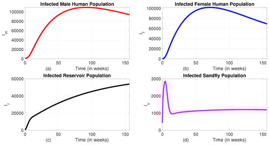
Figure 3.
The dynamics of infected classes without intervention. (a) Infected male human population; (b) Infected female human population; (c) Infected reservoir population; (d) Infected sandfly population.
We can observe from Figure 3 that, in the absence of interventions, the disease continues to spread and remains persistent within the community. This persistence highlights the robustness of the transmission dynamics and the difficulty in achieving natural eradication. Without targeted measures, the disease remains endemic and may lead to long-term health and socioeconomic impacts. Therefore, it becomes essential to implement a range of intervention strategies, such as insecticide-treated bed nets, vector control through indoor residual spraying, treatment programs, and screening and culling of infected reservoirs, to reduce disease prevalence significantly. In the following sections, we will see the impact of different interventions in reducing the number of infected populations.
Despite the ethical concerns, we simulated the total prevalence and corresponding costs to assess the impact of applying control interventions at varying rates for both male and female humans. When the proportion of treatment and ITNs used for the female human population as compared to their male counterpart is set at , , or , there is no significant difference in the total prevalence or intervention costs (see Figure 4). However, when the proportion is reduced to 10%, a noticeable difference in prevalence is observed. Therefore, to optimize resource use and reduce prevalence, it is advisable to take this proportion into consideration.
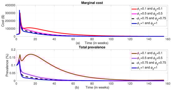
Figure 4.
The dynamics of the total prevalence and control costs at different values of and . (a) Total cost; (b) Total prevalence.
We now analyze the effect of various possible combinations of intervention mechanisms, in reducing the burden of the disease. In each of these combinations, we assumed that only of the controls and are implemented to the female humans. This is based on the information from Figure 4.
Furthermore, to evaluate the impact of reducing the effectiveness of controls on disease prevalence among both male and female human populations, we systematically varied the intensity of the interventions. Assuming that the effectiveness of the controls decay exponentially through time by some rate we multiplied the effect by , where , and 4. To accommodate such a possibility, the expression for in Equation (1) is modified to . Similarly, the death rate of sandflies under control, originally given by in Equation (5), is updated to . Additionally, the treatment rates and , initially defined as and , are now modified to account for a possible decay in effectiveness as and .
The intervention effectiveness variations led to distinct outcomes between male and female populations. Specifically, the prevalence of infection among males remained relatively stable and did not show notable sensitivity to the decreasing levels of intervention effectiveness. In contrast, as illustrated in Figure 5b, Figure 6b, and Figure 7b, the infection prevalence among females demonstrated a marked sensitivity, especially in response to reduced effectiveness of insecticide-treated bed nets and medical treatment.
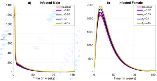
Figure 5.
The role of exponential decay of the effectiveness of insecticide-treated bed net to protect humans from the bite of sandflies. (a) Infected male humans; (b) Infected female humans.
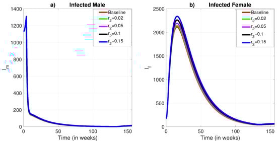
Figure 6.
The role of exponential decay of the effectiveness of insecticide-treated bed net to kill sandflies. (a) Infected male humans; (b) Infected female humans.
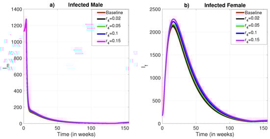
Figure 7.
The role of exponential decay in the effectiveness of medical treatment. (a) Infected male humans; (b) Infected female humans.
When applying identical exponential decay levels to the effectiveness of insecticide spraying, the resulting changes in infection prevalence were minimal for both sexes (see Figure 8b), though a slight impact remained visible among females. Notably, effectiveness reductions of 10% and 15% produced more significant increases in prevalence than smaller reductions, though the overall impact was still moderate.
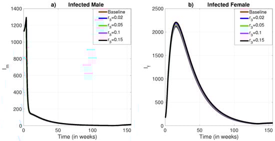
Figure 8.
The role of exponential decay in the effectiveness of insecticide residual spraying. (a) Infected male humans; (b) Infected female humans.
These results suggest that exponential declines in intervention effectiveness, particularly for medical treatment and bed net usage, have a greater impact on the female population. This underscores the importance of incorporating sex-specific considerations into the design and implementation of disease control strategies to ensure equitable and effective health outcomes.
3.1.1. Strategy A (All Controls, i.e., the Combination of the Use of Treated Bed Nets, Vector Control, the Treatment of Infected Individuals, and the Culling of Infected Reservoir Animals)
In this approach, we applied all the four control variables, , , , and , to optimize the objective function J in Equation (12). When comparing Strategy A to the scenario without any control measures, the number of infected male humans (), the infected sandfly population (), and the number of infected reservoirs () show exponential decline (refer to Figure 9a, Figure 9c and Figure 9d, respectively). In contrast, the infected female human population increases for the first about 16 weeks and goes down and becomes optimum at week 130 (Figure 9b). When analyzing the control profile (Figure 9e), it is clear that the first three controls (, , and ) remain at their maximum levels () for approximately 126 weeks. In contrast, the fourth control () remains at the maximum level for the first five weeks and drops from its peak by at the fifth week and gradually decreases to zero by the end of the intervention period.
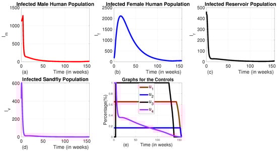
Figure 9.
The dynamics of infected populations with Strategy A and the graph of controls profile. (a) The number of infected male human populations with Strategy A; (b) the number of infected female human populations with Strategy A; (c) the number of infected reservoir populations with Strategy A; (d) the number of infected sandfly populations with Strategy A; and (e) the graph of controls profile.
To assess the influence of each intervention strategy under different levels of implementation efficiency, we conducted a series of simulations, incorporating varying exponential decay rates in control effectiveness. This approach allowed us to explore how gradual reductions in the efficacy of interventions over time affect disease dynamics. For example, when a 10% exponential decline in effectiveness was applied uniformly across all interventions, the results revealed a modest rise in the number of infections among the male human population, while a more pronounced increase was observed among the female population (see Figure 10a,b). Furthermore, the comparative impact of different intervention strategies remained largely unchanged under this moderate decline, indicating similar levels of performance despite the reduced effectiveness. Furthermore, as shown in Figure 10e, lower intervention effectiveness did not lead to a reduction in the duration of maximum control intensity. Instead, it prolonged the application of interventions at their highest possible effort, suggesting that reduced efficiency necessitates sustained maximal efforts to achieve comparable outcomes.
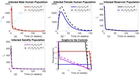
Figure 10.
Time evolution of infected populations under Strategy D, along with the control profiles shown with and without incorporating exponential decay in control effectiveness. (a) The number of infected male human populations with Strategy D; (b) the number of infected female human populations with Strategy D; (c) the number of infected reservoir populations with Strategy D; (d) the number of infected sandfly populations with Strategy D; and (e) the graph of controls profile.
3.1.2. Strategy B (the Combination of the Use of Medical Treatment for Infected Individuals and Animal Culling Without Using Insecticide-Treated Bed Nets or Vector Controls ( and ))
In this strategy, we applied the combination of medical treatment () and culling infected animals () without the use of insecticide-treated bed net () and vector controls (). When comparing Strategy B to an uncontrolled scenario, it can be observed that the population of infected male humans increases during the first 8 weeks, then drops by 62.5% over the following about 4 weeks, then decreases slowly until 133 weeks. Then the number of infected male increases exponentially for the rest of the intervention period (Figure 11a). Similarly, the population of infected female humans initially rises for the first 24 weeks, then decreases until weeks 133 and goes up like the number of males (Figure 11b). This pattern is due to the therapy starting at a low level for the first 8 weeks before reaching its maximum (see Figure 11e). As we can see in Figure 11c,d, although this strategy decreases the number of reservoir and infected sandfly, it cannot decrease these variables to their lowest possible level like that of Strategy A. When the therapy intensifies, the number of infected individuals starts to decrease, but as the treatment level reduces, the infected populations of both male and female humans begin to rise again. Maintaining animal culling at its maximum level for the first 133 weeks ensures that the number of infected reservoirs remains at an optimal low level throughout this period.
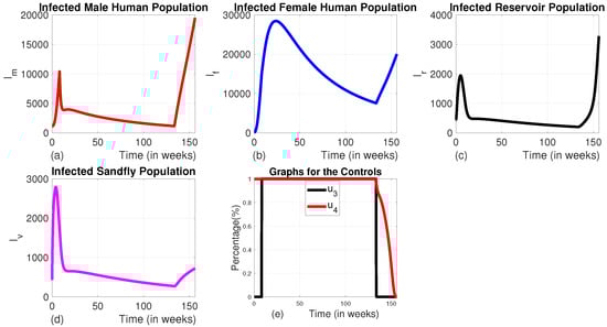
Figure 11.
The dynamics of infected populations with Strategy B and the graph of controls profile. (a) The number of infected male human populations with Strategy B; (b) the number of infected female human populations with Strategy B; (c) the number of infected reservoir populations with Strategy B; (d) the number of infected sandfly populations with Strategy B; and (e) the graph of controls profile.
3.1.3. Strategy C (the Combination of the Use of Insecticide-Treated Bed Nets and Vector Control Without the Use of Medical Treatment and Animal Culling ( and ))
In Strategy C, we employed a combination of insecticide-treated bed nets and vector control, while other interventions like medical treatment and culling of infected animals were set to zero. This strategy results in a significant reduction by of the number of infected human males (Figure 12a) from the baseline by the end of the intervention period. Although it also reduces the number of infected human females significantly (by ) as compared to the scenario without any control measures, the decline is lower than that of human males (Figure 12b). This could be due to the use of the control for the female human population. With the use of this strategy, one can observe that the number of infected vectors and infected reservoirs also decrease by and , respectively, compared to the baseline at the end of the intervention period Figure 12c,d). Figure 12e indicates that the control profile for insecticide-treated bed nets and vector control should continue at their full intensity for the whole planning period.
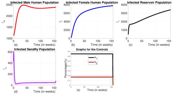
Figure 12.
The dynamics of infected populations with Strategy C and the graph of controls profile. (a) The number of infected male human populations with Strategy C; (b) the number of infected female human populations with Strategy C; (c) the number of infected reservoir populations with Strategy C; (d) the number of infected sandfly populations with Strategy C; and (e) the graphs of the controls profile.
3.1.4. Strategy D (the Combination of Use of Vector Control and Animal Culling Without Insecticide-Treated Bed Nets or Medical Treatment ( and ))
Here, we employed the combination of the use of vector control and animal culling without insecticide-treated bed nets and medical treatment. When comparing the effect of Strategy D to the uncontrolled scenario, there is an exponential decline in the number of infected male and female humans, as well as sandfly populations (see Figure 13a–c). The number of infected reservoirs increases for the first three weeks and decreases until week 14, then rises (Figure 12c). To achieve this, vector control is maintained at its maximum levels for the whole planning period, and animal culling is also at its maximum level for the first 25 weeks before going to the minimum, as shown in Figure 12e).
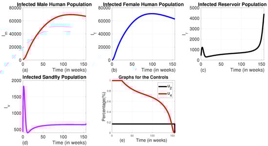
Figure 13.
The dynamics of infected populations with Strategy D and the graph of controls profile. (a) The number of infected male human populations with Strategy D; (b) the number of infected female human populations with Strategy D; (c) the number of infected reservoir populations with Strategy D; (d) the number of infected sandfly populations with Strategy D; and (e) the graph of controls profile.
3.1.5. Strategy E (the Combination of the Use of Insecticide-Treated Bed Nets, Medical Treatment, and Animal Culling Without the Use of Vector Control ())
In this strategy, the combination of the use of ITNs, vector control, and animal culling is employed without the use of medical treatment.
We can observe from Figure 14a–d that this strategy significantly reduces the number of all infected classes like Strategy A. However, it takes a long time for the number of infected sandflies to reach the minimum level as compared to that of Strategy A due to the absence of a vector control strategy in this approach. The number of infected human females also does not reach the minimum possible level in the intervention period as to that of Strategy A. The profile of control graphs is also similar to Strategy A.
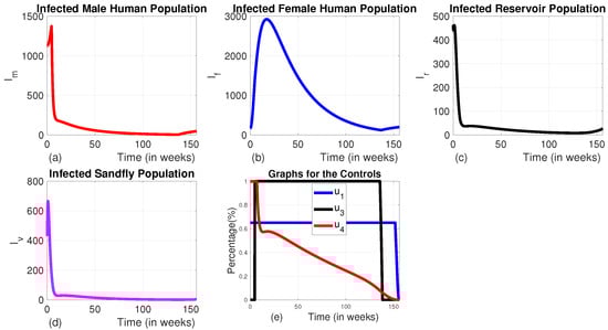
Figure 14.
The dynamics of infected populations with Strategy E and the graph of controls profile. (a) The number of infected human males with Strategy E; (b) the number of infected human females with Strategy E; (c) the number of infected reservoirs with Strategy E; (d) the number of infected sandflies with Strategy E; and (e) the graph of controls profile.
3.1.6. Strategy F (the Combination of the Use of Insecticide-Treated Bed Nets, Vector Control, and Medical Treatment Without the Use of Animal Culling ())
In this approach, we employed the combination of the three controls , , and without using infected animal culling. In this strategy, the number of infected reservoirs increases exponentially for the first 7.8 weeks and then begins to decrease. In contrast, the numbers of infected human males, human females, and sandflies decrease significantly (Figure 15a–d).
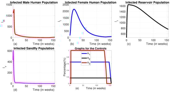
Figure 15.
The dynamics of infected populations with Strategy F and the graph of controls profile. (a) The number of infected human males with Strategy E; (b) the number of infected human females with Strategy E; (c) the number of infected reservoirs with Strategy E; (d) the number of infected sandflies with Strategy E; and (e) the graph of controls profile.
The intervention strategies have been implemented for 156 weeks or three years following the VL data recorded in the study by Awoke et al. [21].
When all control measures are implemented, the total disease prevalence reaches its optimal level. As shown in Figure 16, Strategy F and Strategy E also prove to be effective in reducing the total prevalence, ranking just below Strategy A in terms of the level of total prevalence and their corresponding total cost. On the other hand, Strategy D does not seem to help in controlling the disease, as both the disease prevalence and associated costs increase during the planning period unlike the others. The cost-effectiveness of these strategies will be analyzed in the subsection below.
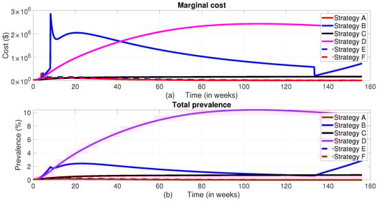
Figure 16.
The dynamics of the total prevalence of the disease and total intervention cost. (a) Total cost; (b) Total Prevalence.
3.1.7. Cost-Effectiveness Analysis of the Proposed Strategies
Cost-effectiveness analysis is a method used to compare the relative costs and outcomes of different interventions or strategies. In the context of optimal control strategies, the cost-effectiveness analysis evaluates whether the benefits achieved by implementing a particular control strategy outweigh its costs. In order to understand the cost-effectiveness of each of the optimal combinations, the incremental cost-effectiveness ratio (ICER) is calculated for each strategy. The incremental cost-effectiveness ratio (ICER) is the additional cost per health outcome [51]. It is the ratio of the difference in total cost between one strategy and the next best alternative to the difference in total number of averted infections through each strategy [47,52]. The number of infections averted is the difference between the total number of infected individuals without control and the total count of infected individuals with control obtained during the control period. To implement the ICER, we simulate the model corresponding to each of the six intervention strategies and apply the formula in Equation (17). Using these simulation results, we rank the control strategies in increasing order of effectiveness based on infection, averted as indicated in Table 3. Accurately estimating the costs associated with interventions that prevent infections and connecting those costs to the Quality of Life Adjusted Years (QALY) gained is crucial for ICER calculation. However, associating the computation of ICER with QALY is complicated due to the indirect costs, opportunity costs, and variations in healthcare systems, as well as other factors. As a result, we did not express ICER in terms of QALY in this study.
Table 3.
Incremental cost-effectiveness ratio in increasing order of total infection averted.
After arranging the strategies in ascending order based on the total infections averted, the incremental cost-effectiveness ratio (ICER) is calculated using the method outlined by [20]. The ICER values are then compared pairwise to identify the most cost-effective strategy.
The pairwise comparisons of the calculated ICER for the different scenarios and corresponding total cost are given in Table 4.
Table 4.
Incremental cost-effectiveness ratio in increasing order of total infection averted.
From ICER of D and ICER of B, it is evident that Strategy B’s ICER is lower than that of Strategy D. This demonstrates that Strategy D is less successful in saving lives and more costly. As a result, Strategy B saves more lives than Strategy D. Strategy D was omitted as a competing strategy, and we calculated the ICER for the remaining strategies, Strategy B, Strategy C, Strategy E, Strategy F, and Strategy A, following the same procedure as in the above, and the results are shown in Table 5.
As we can see from Table 5, when we compare the ICERs of Strategy B and Strategy C, Strategy C has a lower ICER than Strategy B. This shows that Strategy B is strongly dominated by the lower ICER over Strategy C. In other words, compared to Strategy C, Strategy B is less successful and costs more. As a result, Strategy B is excluded in the list of options. Following the same procedures, we have computed the ICERs values as indicated in Table 6.
Table 5.
Incremental cost-effectiveness ratio in increasing order of total infection averted.
Table 6.
Incremental cost-effectiveness ratio in increasing order of total infection averted.
From Table 6, by comparing the ICERs of Strategy C and Strategy E, we can observe that Strategy E has a lower ICER and is hence more cost-effective than Strategy C.
By repeating this process, we can identify the next most cost-effective strategy. From this analysis, Strategy E is found to be the next in line, followed by Strategy F. A final comparison of Strategies F and A shows that Strategy F is strongly dominant, which means it is both more expensive and less effective than Strategy A. Therefore, Strategy A, which is the combination of all four controls, i.e., insecticide-treated bed nets, vector control, treatment of infected human populations, and infected animal culling, emerges as the most cost-effective disease control strategy, as it has the lowest ICER.
To investigate whether incorporating an exponential decay in the effectiveness of control measures alters the cost-effectiveness outcome, we introduced a 10% decay rate to model the gradual reduction in control efficacy over time. We then recalculated the ICERs under this adjusted scenario to reassess and compare the performance of the various intervention strategies. The analysis revealed that the inclusion of decaying effectiveness did not impact the overall ranking of strategies. Specifically, Strategy A, which involves the simultaneous application of all control measures, remained the most cost-effective intervention option, even when accounting for the reduced efficacy over time.
The cost-effectiveness analysis results of this study align with those of a study conducted by Agusto et al. [20], even if our control strategy proposes only of the controls in insecticide-treated bed nets and treatment to be provided to female humans as compared to the ones given to their male counterparts. Their findings indicate that the most cost-effective intervention strategy for controlling the transmission of malaria–VL co-infection involves using personal protection measures, insecticide-treated bed nets, culling infected animal reservoirs, and applying insecticides.
Our findings are consistent with those reported in Zamir et al. [53], where interventions targeting the culling of seropositive dogs led to a direct and rapid reduction in the infectious reservoir population (). However, the study also highlighted that, to sustain this reduction, culling efforts had to be maintained at maximum intensity throughout the intervention period. This aligns closely with the results observed in our study, particularly in Strategy D. In our model, the implementation of both vector control and reservoir culling showed a sharp decline in infection cases during the initial weeks when reservoir culling was applied at maximum intensity. However, once the control effort began to wane, a noticeable resurgence in reservoir infections followed, eventually leading to an increase in total disease prevalence. This similarity underscores the critical importance of maintaining high-intensity reservoir-targeted interventions throughout the control period to prevent disease rebound and highlights the reservoir population’s significant role in the persistence of visceral leishmaniasis.
According to the calculated ICER, Strategy F, which involves all control strategies except animal culling, is the second cost-effective intervention. This finding is consistent with the results of Zhao et al. [18], who state that animal culling is an ineffective VL control strategy. The third most cost-effective strategy, according to our comparison result, includes using insecticide-treated bed nets, medical treatment, and animal culling without using vector control or Strategy E.
4. Conclusions
In this paper, a mathematical model for the dynamics of sex-structured visceral leishmaniasis transmission model is presented and analyzed. We have added four time-dependent control variables to establish optimal disease control strategies. These control variables include treating infected male and female human populations, vector control, using bed nets treated with insecticide, and the culling of infected animals. The positivity and boundedness of the solution, as well as the basic reproduction number with constant control, are computed. We derived and analyzed the necessary conditions for the optimal control problem by using Pontryagin’s Maximum Principle. The numerical simulations show that the overall prevalence of the disease will decrease over time with the inclusion of each of these control techniques into the model. Cost-effectiveness analysis is employed to evaluate the economic implications of the various combinations of the four control measures for VL. To investigate the cost-effectiveness of every possible strategies, we have computed the incremental cost-effectiveness ratio (ICER). We performed a pairwise comparison of the ICER of each strategy and identified the strategy with a smaller ICER, which averts more infections in humans and utilizes the smallest possible cost of intervention.
The result shows a comprehensive evaluation of various intervention strategies aimed at reducing disease transmission and prevalence. The findings show that the most effective and cost-efficient approach is Strategy A, which combines all the four key controls: insecticide-treated bed nets, vector control, medical treatment of infected individuals, and culling of infected animal reservoirs. This strategy leads to a significant and sustained reduction in the number of infected male and female humans, vectors (e.g., sandflies), and animal reservoirs. The intervention’s success is attributed to the simultaneous targeting of multiple transmission pathways, ensuring that disease prevalence decreases rapidly and remains low throughout the intervention period.
Cost-effectiveness analysis, using the incremental cost-effectiveness ratio (ICER), further validates Strategy A as the optimal solution, providing the greatest reduction in disease prevalence for the lowest cost. Strategy E, which excludes vector control, and Strategy F, which omits animal culling, are also effective but rank lower in cost-effectiveness. These strategies reduce disease prevalence but do not achieve the same level of control as Strategy A. The study highlights that strategies like Strategy B (medical treatment and culling without bed nets or vector control) and Strategy D (vector control and culling without bed nets or medical treatment) are less efficient. Although they reduce some components of the infected population, they fail to maintain low infection levels over the intervention period and are more costly, making them suboptimal.
Our findings emphasize the importance of a multi-pronged approach for VL control. Strategies that focus on just one or two interventions, or that limit the application of controls to certain populations, are less successful and more expensive in the long term. The analysis was performed by applying a 50% control strategy to the female humans, compared to their male counterparts. As can be seen from the evaluation, it can still effectively eliminate the burden of VL from the entire population within the planning period. Integrated intervention strategies like Strategy A provide the most effective means of reducing both disease prevalence and long-term socioeconomic impacts. Furthermore, the study underscores the need for a careful balance between cost and effectiveness, as shown by the ICER analysis, to optimize resource allocation in public health programs to control persistent infectious diseases. It is important to note that the scenarios involving unequal allocation of interventions between sexes are considered purely for methodological exploration. In practice, equitable access to control measures such as treatment and ITNs is critical, particularly in settings where women may face increased exposure or barriers to healthcare. The second limitation of this study is that it is based on a deterministic modeling framework, which does not account for possible environmental noises. Operational constraints, such as the durability of bed nets, variations in treatment adherence, and delays in implementation, were not explicitly incorporated into the model. Future research should aim to extend this work by developing a stochastic version of the model that integrates these real-world complexities, to better capture uncertainty and improve the applicability of the results to public health planning. In this study, ICER was expressed in terms of infections averted rather than QALYs, due to the lack of established utility weights for VL and the complexity of capturing indirect and opportunity costs across varying healthcare systems, while the ICER approach provides useful comparative insights, it does not fully capture the health-related quality of life benefits associated with each intervention. In future work, we aim to extend our economic analysis by incorporating QALY-based metrics in collaboration with health economists, to offer a more comprehensive evaluation aligned with standard health economic practices.
Author Contributions
Conceptualization, S.M.K. and T.D.A.; Methodology, T.D.A. and S.M.K.; Software, T.D.A. and S.M.K.; Validation, T.D.A., S.M.K. and G.M.T.; Formal analysis, T.D.A.; Investigation, T.D.A.; Writing—original draft, T.D.A.; Writing—review and editing, T.D.A., S.M.K., K.S.M. and G.M.T.; Supervision, S.M.K., K.S.M. and G.M.T.; Funding acquisition, G.M.T.; Project administration, K.S.M. All authors have read and agreed to the published version of the manuscript.
Funding
This research was funded by O.R. Tambo Africa Research Chairs Initiative as supported by the Botswana International University of Science and Technology, the Ministry of Tertiary Education, Science, and Technology; the National Research Foundation of South Africa (NRF); the Department of Science and Innovation of South Africa (DSI); the International Development Research Centre of Canada (IDRC); and the Oliver and Adelaide Tambo Foundation (OATF), with grant number: (UID)136696.
Data Availability Statement
Data are contained within the article.
Acknowledgments
The authors would like to express sincere gratitude to the editor and anonymous reviewers for their valuable time, insightful comments, and constructive suggestions that significantly improved the quality and clarity of this manuscript.
Conflicts of Interest
The authors declare no conflicts of interest.
References
- Wamai, R.G.; Kahn, J.; McGloin, J.; Ziaggi, G. Visceral leishmaniasis: A global overview. J. Glob. Health Sci. 2020, 2. [Google Scholar] [CrossRef]
- Desjeux, P. The increase in risk factors for leishmaniasis worldwide. Trans. R. Soc. Trop. Med. Hyg. 2001, 95, 239–243. [Google Scholar] [CrossRef] [PubMed]
- Lockard, R.D.; Wilson, M.E.; Rodríguez, N.E. Sex-related differences in immune response and symptomatic manifestations to infection with Leishmania species. J. Immunol. Res. 2019, 2019, 4103819. [Google Scholar] [CrossRef] [PubMed]
- Moncaz, A.; Faiman, R.; Kirstein, O.; Warburg, A. Breeding sites of Phlebotomus sergenti, the sandfly vector of cutaneous leishmaniasis in the Judean Desert. PLoS Neglected Trop. Dis. 2012, 6, e1725. [Google Scholar] [CrossRef]
- Alexander, B.; Maroli, M. Control of phlebotomine sandflies. Med. Vet. Entomol. 2003, 17, 1–8. [Google Scholar] [CrossRef]
- Maroli, M.; Khoury, C. Prevention and control of leishmaniasis vectors: Current approaches. Parassitologia 2004, 46, 211–215. [Google Scholar] [CrossRef] [PubMed]
- Montenegro, Q.C.A.; Runge-Ranzinger, S.; Rahman, K.M.; Horstick, O. Effectiveness of vector control methods for the control of cutaneous and visceral leishmaniasis: A meta-review. PLoS Neglected Trop. Dis. 2021, 15, e0009309. [Google Scholar] [CrossRef]
- Alvar, J.; Vélez, I.D.; Bern, C.; Herrero, M.; Desjeux, P.; Cano, J.; Jannin, J.; Boer, M.D. WHO Leishmaniasis Control Team. Leishmaniasis worldwide and global estimates of its incidence. PLoS ONE 2012, 7, e35671. [Google Scholar] [CrossRef]
- ELmojtaba, I.M. Mathematical model for the dynamics of visceral leishmaniasis–Malaria co-infection. Math. Methods Appl. Sci. 2016, 39, 4334–4353. [Google Scholar] [CrossRef]
- Shimozako, H.J.; Wu, J.; Massad, E. Mathematical modelling for Zoonotic Visceral Leishmaniasis dynamics: A new analysis considering updated parameters and notified human Brazilian data. Infect. Dis. Model. 2017, 2, 143–160. [Google Scholar] [CrossRef]
- Biswas, S. Mathematical modeling of visceral leishmaniasis and control strategies. Chaos Solitons Fractals 2017, 104, 546–556. [Google Scholar] [CrossRef]
- Rock, K.S.; le Rutte, E.A.; de Vlas, S.J.; Adams, E.R.; Medley, G.F.; Hollingsworth, T.D. Uniting mathematics and biology for control of visceral leishmaniasis. Trends Parasitol. 2015, 31, 251–259. [Google Scholar] [CrossRef]
- Subramanian, A.; Singh, V.; Sarkar, R.R. Understanding visceral leishmaniasis disease transmission and its control—A study based on mathematical modeling. Mathematics 2015, 3, 913–944. [Google Scholar] [CrossRef]
- Zou, L.; Chen, J.; Ruan, S. Modeling and analyzing the transmission dynamics of visceral leishmaniasis. Math. Biosci. Eng. 2017, 14, 1585–1604. [Google Scholar] [CrossRef]
- Song, H.; Tian, D.; Shan, C. Modeling the effect of temperature on dengue virus transmission with periodic delay differential equations. Math. Biosci. Eng. 2020, 17, 4147–4164. [Google Scholar] [CrossRef]
- Biswas, D.; Dolai, S.; Chowdhury, J.; Roy, P.K.; Grigorieva, E.V. Cost-Effective Analysis of Control Strategies to Reduce the Prevalence of Cutaneous Leishmaniasis, Based on a Mathematical Model. Math. Comput. Appl. 2018, 23, 38. [Google Scholar] [CrossRef]
- Pantha, B.; Agusto, F.B.; Elmojtaba, I.M. Optimal control applied to a visceral leishmaniasis model. Electron. J. Differ. 2020, 80, 1–24. [Google Scholar] [CrossRef]
- Zhao, S.; Kuang, Y.; Wu, C.H.; Ben-Arieh, D.; Ramalho-Ortigao, M.; Bi, K. Zoonotic visceral leishmaniasis transmission: Modeling, backward bifurcation, and optimal control. J. Math. Biol. 2016, 73, 1525–1560. [Google Scholar] [CrossRef]
- Ghosh, I.; Sardar, T.; Chattopadhyay, J. A mathematical study to control visceral leishmaniasis: An application to South Sudan. Bull. Math. Biol. 2017, 79, 1100–1134. [Google Scholar] [CrossRef]
- Agusto, F.B.; ELmojtaba, I.M. Optimal control and cost-effective analysis of malaria/visceral leishmaniasis co-infection. PLoS ONE 2017, 12, e0171102. [Google Scholar] [CrossRef]
- Awoke, T.D.; Kassa, S.M.; Morupisi, K.S.; Tsidu, G.M. Sex-structured disease transmission model and control mechanisms for visceral leishmaniasis (VL). PLoS ONE 2024, 19, e0301217. [Google Scholar] [CrossRef] [PubMed]
- DebRoy, S.; Prosper, O.; Mishoe, A.; Mubayi, A. Challenges in modeling complexity of neglected tropical diseases: A review of dynamics of visceral leishmaniasis in resource limited settings. Emerg. Themes Epidemiol. 2017, 14, 1–4. [Google Scholar] [CrossRef] [PubMed]
- Stockdale, L.; Newton, R. A review of preventative methods against human leishmaniasis infection. PLoS Neglected Trop. Dis. 2013, 7, e2278. [Google Scholar] [CrossRef] [PubMed]
- Maia, C.; Dantas-Torres, F.; Campino, L. Parasite Biology: The Reservoir Hosts. In The Leishmaniases: Old Neglected Tropical Diseases; Bruschi, F., Gradoni, L., Eds.; Springer Nature: Gewerbestrasse, Switzerland, 2018; pp. 79–106. [Google Scholar]
- World Health Organization, VL Fact Sheet. Available online: https://www.who.int/news-room/fact-sheets/detail/leishmaniasis (accessed on 16 April 2024).
- Chapman, L.A.; Dyson, L.; Courtenay, O.; Chowdhury, R.; Bern, C.; Medley, G.F.; Hollingsworth, T.D. Quantification of the natural history of visceral leishmaniasis and consequences for control. Parasites Vectors 2015, 8, 1–3. [Google Scholar] [CrossRef]
- Asfaw, M.D.; Buonomo, B.; Kassa, S.M. Impact of human behavior on ITNs control strategies to prevent the spread of vector borne diseases. Atti della Accademia Peloritana dei Pericolanti-Classe di Scienze Fisiche. Mat. Enaturali 2018, 96, 2. [Google Scholar] [CrossRef]
- Malaria Consortium. Leishmaniasis Control in Eastern Africa: Past and Present Efforts and Future Needs; Situation and Gap Analysis; Malaria Consortium: London, UK, 2010; Volume 86. [Google Scholar]
- Balaska, S.; Fotakis, E.A.; Chaskopoulou, A.; Vontas, J. Chemical control and insecticide resistance status of sandfly vectors worldwide. PLoS Neglected Trop. Dis. 2021, 15, e0009586. [Google Scholar] [CrossRef]
- Joshi, A.B.; Das, M.L.; Akhter, S.; Chowdhury, R.; Mondal, D.; Kumar, V.; Das, P.; Kroeger, A.; Boelaert, M.; Petzold, M. Chemical and environmental vector control as a contribution to the elimination of visceral leishmaniasis on the Indian subcontinent: Cluster randomized controlled trials in Bangladesh, India and Nepal. BMC Med. 2009, 7, 1–9. [Google Scholar] [CrossRef]
- Wilson, A.L.; Courtenay, O.; Kelly-Hope, L.A.; Scott, T.W.; Takken, W.; Torr, S.J.; Lindsay, S.W. The importance of vector control for the control and elimination of vector-borne diseases. PLoS Neglected Trop. Dis. 2020, 14, e0007831. [Google Scholar] [CrossRef]
- Ahmed, B.N.; Nabi, S.G.; Rahman, M.; Selim, S.; Bashar, A.; Rashid, M.M.; Lira, F.Y.; Choudhury, T.A.; Mondal, D. Kala-azar (visceral leishmaniasis) elimination in Bangladesh: Successes and challenges. Curr. Trop. Med. Rep. 2014, 1, 163–169. [Google Scholar] [CrossRef]
- Matlashewski, G.; Arana, B.; Kroeger, A.; Battacharya, S.; Sundar, S.; Das, P.; Sinha, P.K.; Rijal, S.; Mondal, D.; Zilberstein, D.; et al. Visceral leishmaniasis: Elimination with existing interventions. Lancet Infect. Dis. 2011, 11, 322–325. [Google Scholar] [CrossRef]
- Costa, C.H. How effective is dog culling in controlling zoonotic visceral leishmaniasis? A critical evaluation of the science, politics and ethics behind this public health policy. Rev. Soc. Bras. Med. Trop. 2011, 44, 232–242. [Google Scholar] [CrossRef] [PubMed][Green Version]
- Van den Driessche, P.; Watmough, J. Reproduction numbers and sub-threshold endemic equilibria for compartmental models of disease transmission. Math. Biosci. 2002, 180, 29–48. [Google Scholar] [CrossRef] [PubMed]
- Fleming, W.H.; Rishel, R.W. Deterministic and Stochastic Optimal Control, 1st ed.; Springer: New York, NY, USA; Berlin/Heidelberg, Germany, 2012. [Google Scholar]
- Kassa, S.M.; Hove-Musekwa, S.D. Optimal control of allocation of resources and the economic growth in HIV-infected communities. Optim. Control Appl. Methods 2014, 35, 627–646. [Google Scholar] [CrossRef]
- Earl, A.C.; Norman, L.; Teichmann, T. Theory of Ordinary Differential Equations. Phys. Today 1956, 9, 18. [Google Scholar] [CrossRef]
- Barbu, V.; Precupanu, T. Convexity and Optimization in Banach Spaces; Springer Science & Business Media: New York, NY, USA, 2012. [Google Scholar]
- Pedregal, P. Variational Problems and Dynamic Programming. In Introduction to Optimization. Texts in Applied Mathematics; Marsden, J.E., Sirovich, L., Antman, S.S., Eds.; Springer: New York, NY, USA, 2004; Volume 46, pp. 137–194. [Google Scholar]
- Awoke, T.D.; Kassa, S.M. Optimal control strategy for TB-HIV/AIDS Co-infection model in the presence of behaviour modification. Processes 2018, 6, 48. [Google Scholar] [CrossRef]
- Fister, K.R.; Lenhart, S.; McNally, J.S. Optimizing chemotherapy in an hiv model. Electron. J. Differ. Equ. 1998, 1998, 1–12. [Google Scholar]
- Gaff, H.; Schaefer, E. Optimal control applied to vaccination and treatmentstrategies for various epidemiological models. Math. Biosci. Eng. 2009, 6, 469–492. [Google Scholar] [CrossRef]
- Kassa, S.M.; Ouhinou, A. The impact of self-protective measures in the optimal interventions for controlling infectious diseases of human population. J. Math. Biol. 2015, 70, 213–236. [Google Scholar] [CrossRef]
- Blayneh, K.W.; Gumel, A.B.; Lenhart, S.; Clayton, T. Backward bifurcation and optimal control in transmission dynamics of West Nile virus. Bull. Math. Biol. 2010, 72, 1006–1028. [Google Scholar] [CrossRef]
- Lenhart, S.; Workman, J.T. Optimal Control Applied to Biological Models, 1st ed.; Chapman and Hall/CRC: New York, NY, USA, 2007. [Google Scholar]
- Berhe, H.W.; Makinde, O.D.; Theuri, D.M. Co-dynamics of measles and dysentery diarrhea diseases with optimal control and cost-effectiveness analysis. Appl. Math. Comput. 2019, 347, 903–921. [Google Scholar] [CrossRef]
- Chappuis, F.; Sundar, S.; Hailu, A.; Ghalib, H.; Rijal, S.; Peeling, R.W.; Alvar, J.; Boelaert, M. Visceral leishmaniasis: What are the needs for diagnosis, treatment and control? Nat. Rev. Microbiol. 2007, 5, 873–882. [Google Scholar] [CrossRef] [PubMed]
- Srinivasan, R.; Panicker, K.N. Laboratory observations on the biology of the phlebotomid sandfly, Phlebotomus papatasi (Scopoli, 1786). Southeast Asian J. Trop. Med. Public Health 1993, 24, 536–539. [Google Scholar] [PubMed]
- Alvar, J.; Molina, R.; San Andrés, M.; Tesouro, M.; Nieto, J.; Vitutia, M.; González, F.; San Andrés, M.D.; Boggio, J.; Rodriguez, F.; et al. Canine leishmaniasis: Clinical, parasitological and entomological follow-up after chemotherapy. Ann. Trop. Med. Parasitol. 1994, 88, 371–378. [Google Scholar] [CrossRef] [PubMed]
- Agusto, F.B. Optimal isolation control strategies and cost-effectiveness analysis of a two-strain avian influenza model. Biosystems 2013, 113, 155–164. [Google Scholar] [CrossRef]
- Workineh, Y.H.; Kassa, S.M. Optimal control of the spread of meningitis: In the presence of behaviour change of the society and information dependent vaccination. Commun. Math. Biol. Neurosci. 2021, 2021, 29. [Google Scholar] [CrossRef]
- Zamir, M.; Nadeem, F.; Zaman, G. Optimal control of visceral, cutaneous and post kala-azar leishmaniasis. Adv. Differ. Equ. 2020, 1, 548. [Google Scholar] [CrossRef]
Disclaimer/Publisher’s Note: The statements, opinions and data contained in all publications are solely those of the individual author(s) and contributor(s) and not of MDPI and/or the editor(s). MDPI and/or the editor(s) disclaim responsibility for any injury to people or property resulting from any ideas, methods, instructions or products referred to in the content. |
© 2025 by the authors. Licensee MDPI, Basel, Switzerland. This article is an open access article distributed under the terms and conditions of the Creative Commons Attribution (CC BY) license (https://creativecommons.org/licenses/by/4.0/).