Research on E-Commerce Inventory Sales Forecasting Model Based on ARIMA and LSTM Algorithm

Abstract

Accurate forecasting is critical for effective warehouse network planning and inventory management in e-commerce. This study tackles these challenges by applying a differentiated forecasting strategy over a three-month period. The Autoregressive Integrated Moving Average (ARIMA) model is used for monthly inventory predictions, while the Long Short-Term Memory (LSTM) neural network is employed for daily sales forecasts. Experimental validation across 350 product categories demonstrates the efficacy of this approach. ARIMA effectively captured dynamic inventory trends (e.g., Category 1 showing gradual increases; Category 91 depleting from 3824 to 0). Concurrently, LSTM successfully modeled complex daily sales fluctuations (e.g., Category 61 peaking at 3693 units on 21 July; Category 31 consistently recording zero sales). This dual-model strategy, leveraging the complementary strengths of ARIMA for relatively stable monthly inventory series and LSTM for volatile daily sales patterns, provides a robust, data-driven basis for optimizing warehouse resource planning and product category allocation. Furthermore, visualization of categorized forecast results reveals distinct sales distribution patterns, thereby enabling enterprises to refine inventory and sales strategies with greater precision, leading to reduced redundant space investment and improved resource allocation efficiency. Future research will focus on incorporating multivariate interactions to further enhance model practicality and predictive power.

1. Introduction

In the rapidly evolving landscape of modern e-commerce, efficient warehouse management has emerged as a critical determinant of business success. As operations scale and product diversity burgeons, the complexity of warehouse management intensifies [1]. To navigate this, enterprises increasingly adopt distributed warehouse cluster models, systematically classifying goods by attributes like category and packaging to refine inventory control and optimize operational efficiency [2,3]. Crucially, the efficacy of such sophisticated management hinges upon precise inventory and sales forecasting. Accurate forecasts provide a scientific basis for strategic warehouse zoning (e.g., allocating specific areas for distinct product categories based on predicted turnover), enabling proactive resource planning, minimizing redundant space investment, and reducing overall operating costs, thereby securing a competitive edge [4]. However, achieving the requisite forecasting accuracy, particularly across diverse product categories with varying demand dynamics, presents a substantial and persistent challenge.

The dynamic and volatile nature of the e-commerce sales environment, fueled by advancements in Big Data and Internet technologies, presents formidable challenges for traditional time series forecasting methods. Conventional algorithms often struggle to capture the nonlinear and high-frequency fluctuations characteristic of modern sales data, necessitating the exploration of more sophisticated modeling techniques [5,6]. In response, researchers have investigated various predictive models. For instance, Raizada et al. [7] benchmarked supervised learning algorithms for sales estimation across Walmart stores. Zhang et al. [8] improved e-commerce sales prediction accuracy using ensemble methods like random forests and GBDT. For inventory, Chai et al. [9] applied LSTM to predict agricultural equipment stock, while Huang et al. [10] utilized an improved PSO model for automated warehouse inventory, enhancing utilization. Feng et al. [11] demonstrated a BP neural network’s higher accuracy for product sales prediction. While these studies showcase valuable advancements, a critical gap remains in developing integrated forecasting solutions tailored to the distinct characteristics of e-commerce operations—specifically, the need to simultaneously address the relative stability of (often monthly) inventory data and the pronounced volatility of (often daily) sales data across a multitude of product categories. This necessitates a differentiated modeling approach.

Responding directly to the need for a differentiated modeling approach identified above, this study proposes and empirically evaluates an innovative dual-model forecasting framework to address inventory and sales forecasting challenges within e-commerce warehousing networks. Leveraging operational data from 350 product categories over a three-month period (July–September), our research aims to enhance predictive accuracy and practical applicability. The main contributions are threefold:

• Strategic Differentiation of Forecasting Targets: We precisely define and separate forecasting objectives: “inventory” represents overall monthly stocking requirements (reflecting replenishment cycles and storage capacity planning), while “sales” denote daily total shipments (capturing volatile customer demand). This delineation is crucial for tailoring models to the distinct temporal characteristics and business implications of each metric.
• Application of a Complementary Dual-Model Strategy: To effectively model these differentiated targets, we strategically apply ARIMA models for their proficiency in capturing seasonality and trends in relatively stable monthly inventory data, and LSTM networks for their strength in handling non-linear, high-frequency fluctuations inherent in daily sales data. This tailored combination is shown to yield significant improvements in forecasting accuracy.
• Demonstration of Practical Value for Warehouse Operations: Beyond theoretical model optimization, this research underscores the practical utility of the framework. Through multi-dimensional evaluation metrics, we provide a quantitative basis for enhanced warehouse planning decisions, including optimizing category-specific warehouse layouts, reducing inventory holding costs, and improving supply chain responsiveness.

2. Materials and Methods

2.1. ARIMA Model

The Autoregressive Integrated Moving Average (ARIMA) algorithm [12] is a classic time series prediction method primarily used for analyzing and predicting univariate time series data. It models the dynamic characteristics of time series by combining three main components: autoregression (AR), integration (I) achieved through differencing, and moving average (MA).

The essence of the ARIMA model is the combination of an appropriate level of differencing applied to the original non-stationary series $X_t$ to make it stationary, and then modeling this stationary series with an ARMA model. It is denoted as ARIMA(p, d, q). Let $X_t$ represent the original time series data. The d-th order-differenced series, $Y_t={\Delta }^d{X}_t$, is then modeled. The ARIMA(p, d, q) model can be expressed as

$${\Delta }^d{X}_t={\displaystyle \sum _{i=1}^p{\varphi }_i{\Delta }^d{X}_{t-i}+{\epsilon }_t-{\displaystyle \sum _{j=1}^q{\theta }_j{\epsilon }_{t-j}}}$$

(1)

where p is the order of the autoregressive (AR) part, d is the order of differencing (the “Integrated” part), and q is the order of the moving average (MA) part. ${\epsilon }_t$ is an independent identically distributed white noise sequence with zero mean and constant variance. B is the lag operator, defined by

$$B^n{X}_t=X_{t-1}$$

(2)

The autoregressive polynomial $\varphi (B)$ and the moving average polynomial $\theta (B)$ are given by

$$\varphi (B)=1-{\displaystyle \sum _{i=1}^p{\varphi }_i{B}^i}$$

(3)

$$\theta (B)=1-{\displaystyle \sum _{i=1}^q{\theta }_j{B}^j}$$

(4)

Using these definitions, Equation (1) is equivalent to the common compact form $\varphi (B){\Delta }^d{X}_t=\theta (B){\epsilon }_t$.

The key point of establishing an ARIMA(p, d, q) model is the selection of the three parameters (p, d, q). d is the order of differencing required to transform the original non-stationary observation series into a stationary time series. The appropriate value of d is typically determined by examining the Autocorrelation Function (ACF) plot of the series and/or using statistical tests such as the Augmented Dickey–Fuller (ADF) test to check for stationarity after differencing. Once d is determined and the series is stationary, the model selection process for p and q includes analyzing the ACF and partial autocorrelation function (PACF) plots of the differenced series to suggest candidate values. Final selection among candidate (p, q) combinations (and potentially d if multiple differencing orders yield stationarity) is often guided by information criteria. In this paper, the Bayesian Information Criterion (BIC) is used for this purpose. BIC provides an approximation for the model evidence and is calculated as follows:

$$BIC=p\ln (N)-2\ln (L)$$

(5)

where L is the maximized value of the likelihood function for the estimated model, N is the number of effective observations used for estimation (after differencing), and the term “p” in this BIC formula represents the total number of estimated parameters in the model (e.g., $p_{AR}+q_{MA}$ plus a constant if included), not to be confused with the AR order p from ARIMA(p, d, q).

In this research, ARIMA is applied to monthly inventory data due to its effectiveness in modeling trends (addressed by differencing) and autocorrelations (seasonal or otherwise, captured by AR and MA components) typical of such series in warehousing demand.

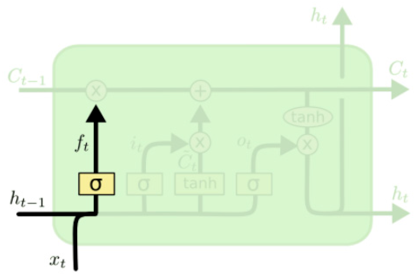
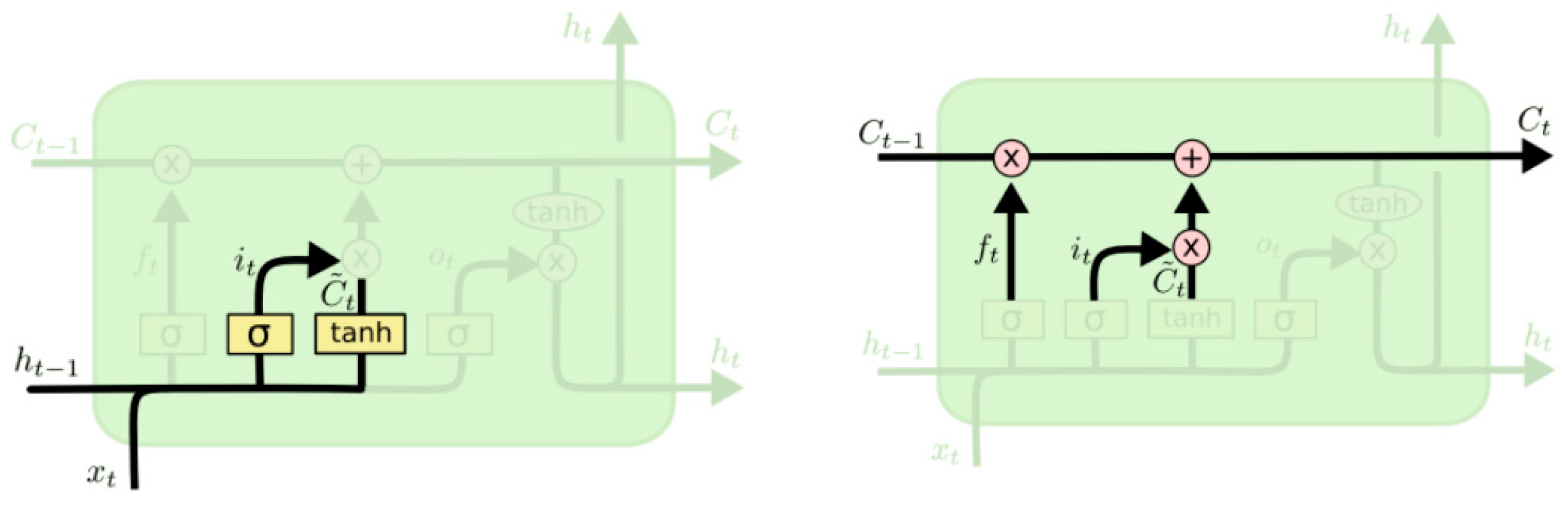
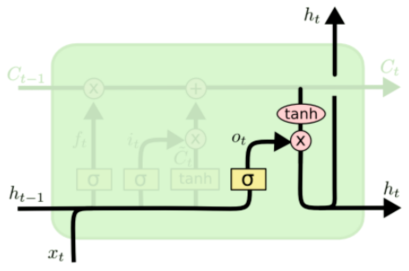
2.2. LSTM Model

Traditional Recurrent Neural Networks (RNNs), while capable of processing sequential data, often struggle with learning long-term dependencies due to issues like vanishing or exploding gradients. The Long Short-Term Memory (LSTM) network, an advanced RNN architecture, was proposed to overcome these limitations [13,14]. LSTM networks introduce a memory cell capable of maintaining information over extended time intervals, making them particularly effective for tasks involving long sequences.

LSTMs address the long-term dependency problem by incorporating a sophisticated gating mechanism. This allows them to selectively remember or forget information, effectively transmitting relevant information through long time series and mitigating the gradient vanishing/exploding problem [15]. While LSTM retains the chained structure of RNNs, its repeating module has a more complex internal structure, typically involving a cell state and three primary gates: the forget gate, the input gate, and the output gate. Figure 1 illustrates the general architecture of an LSTM unit.

The diagrams for the individual gates (Figure 2, Figure 3 and Figure 4) use specific conventions: each line represents a complete vector flowing from one node to another; pink circles denote element-wise operations (e.g., vector addition or multiplication); yellow boxes represent learned neural network layers.

Forget Gate: The first step in the LSTM cell is to decide what information to discard from the cell state. This decision is made by the “forget gate” layer (Figure 2). It takes the previous hidden state $h_{t-1}$ and the current input $x_t$, and a sigmoid function outputs a number $f_t$ between 0 and 1 for each number in the previous cell state $C_{t-1}$. A value of 1 means “completely keep this”, while a value of 0 means “completely get rid of this”.

$$f_t=\sigma (W_f\cdot [x_t,h_{t-1}]+b_f)$$

(6)

Input Gate (Memory Gate): The next step is to decide what new information will be stored in the cell state. This has two parts, managed by what is termed the “memory gate” layer (Figure 3). First, a sigmoid layer called the “input gate layer” $i_t$ decides which values to update. Second, a tanh layer creates a vector of new candidate values, ${\tilde{C}}_t$, that could be added to the state.

$$i_t=\sigma (W_i\cdot [x_t,h_{t-1}]+b_i)$$

(7)

$${\tilde{C}}_t=\tanh (W_C\cdot [x_t,h_{t-1}]+b_C)$$

(8)

Cell State Update: With the outputs from the forget gate $f_t$ and the input gate $i_t\cdot C_t$, the old cell state $C_t$ is updated to the new cell state $C_t$. The old state is multiplied by $f_t$ (forgetting things decided earlier), and then $i_t\cdot C_t$ is added (the new candidate values, scaled by how much to update each state value).

Output Gate: Finally, the output gate layer (Figure 4) determines the next hidden state, $h_t$. This output is a filtered version of the cell state. First, a sigmoid layer $o_t$ decides which parts of the cell state will be output. Then, the cell state $C_t$ is passed through a tanh function (to scale values between −1 and 1) and multiplied by the output of the sigmoid gate $o_t$.

$$o_t=\sigma (W_o\cdot [h_{t-1},x_t]+b_o)$$

(9)

$$C_t=f_t\cdot C_{t-1}+i_t\cdot {\tilde{C}}_t$$

(10)

$$h_t=o_t\cdot \tanh (C_t)$$

(11)

LSTM’s ability to selectively retain and forget information through these gating mechanisms makes it well-suited for modeling the nonlinear, high-frequency, and potentially complex temporal patterns often seen in e-commerce daily sales data. In this study, LSTM is utilized to forecast the sales of each product category on a daily basis, aiming to capture short-term trends and irregular fluctuations, such as those caused by promotional surges or market shocks.

3. Experimental Results and Analysis

3.1. Experimental Environment and Data Set

The experimental analysis was conducted using Python 3.8 on a Windows 11 operating system. The dataset, provided by the 2024 Mathorcup Big Data Competition, encompasses transactional and inventory data for 350 product categories. Each record contains a category ID, monthly inventory levels, daily sales figures, and corresponding timestamps, spanning a period consistent with the three-month forecasting horizon (July–September) discussed earlier. This dataset offers a diverse range of sales and inventory behaviors, providing a robust foundation for rigorous testing of forecasting performance across categories with varying demand dynamics.

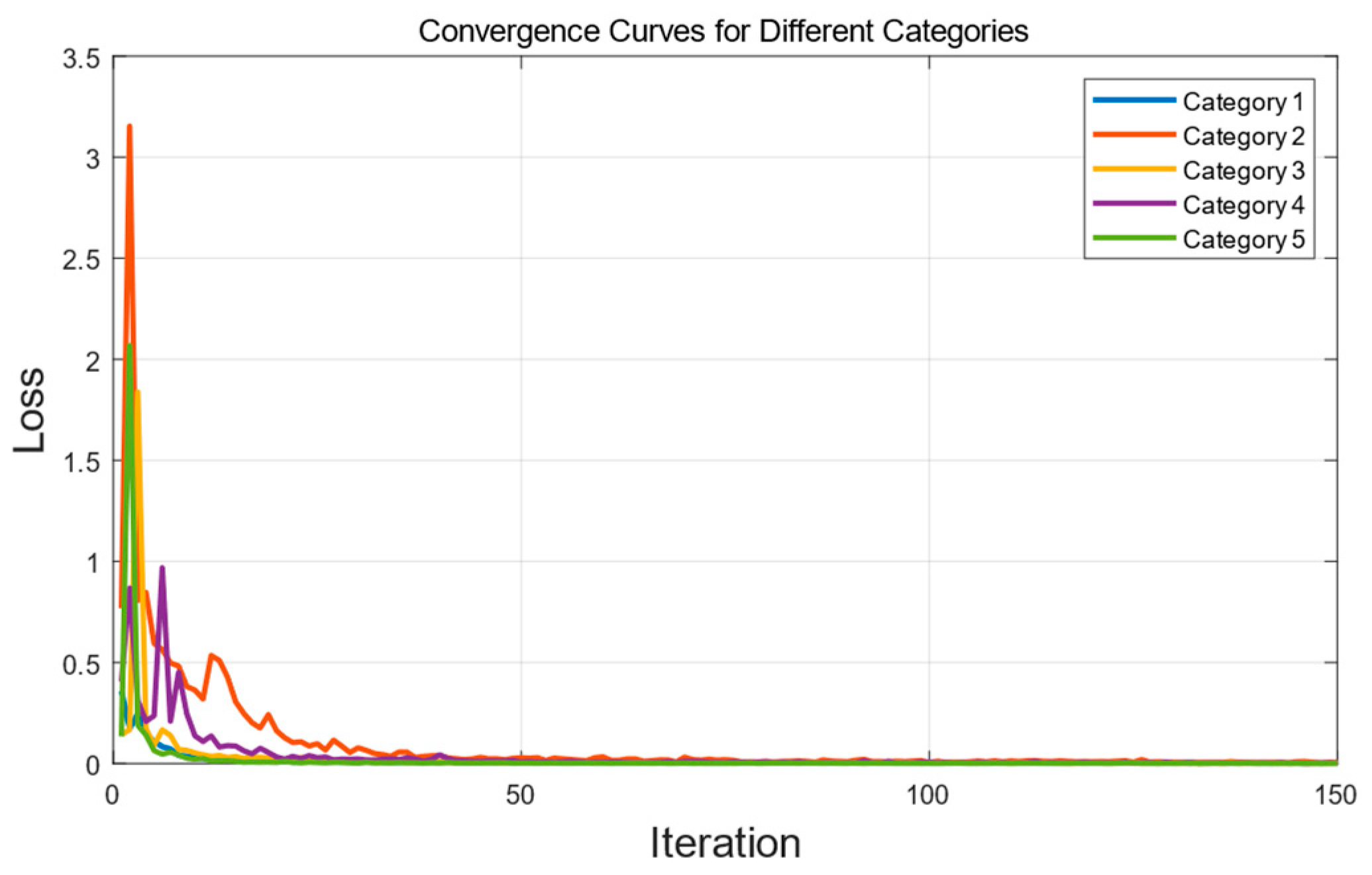
3.2. Model Convergence

Figure 5 presents the training loss curves for the LSTM model across a representative selection of five product categories. As illustrated, the training loss for each of these categories consistently decreases and stabilizes over iterations. This behavior indicates that the models achieved good convergence and suggests effective parameter optimization during the training phase. Ideally, Figure 5 would also display the corresponding validation loss curves for each category. The comparison between training and validation loss is crucial for definitively assessing model generalizability and diagnosing potential overfitting. While not explicitly shown here, the stabilization of the training loss, assuming it is complemented by a similarly stable or decreasing validation loss (monitored during the actual training process as per standard practice), would support the conclusion that the model has learned meaningful patterns without significant overfitting.

3.3. Inventory Forecast Results Based on the ARIMA Algorithm

The ARIMA model is applied to forecast the monthly inventory levels for the 350 product categories. The resulting three-month projections for a selection of categories are presented in

Table 1. Inventory forecast results for selected categories (units).

	July	August	September
category 1	6076	6119	6174
category 31	0	0	0
category 61	240,564	240,564	240,564
category 91	3824	951	0
category 121	73,618	73,618	73,618
category 151	100,857	129,028	110,154
category 181	379	763	433
category 211	8211	8560	8498
category 241	58,047	58,047	58,047
category 271	15,108	15,108	15,108
category 301	2528	2635	2644
category 331	39,559	25,879	12,198

. These forecasts reveal diverse inventory trajectories, offering crucial data points for warehousing planning and resource allocation.

As evidenced in Table 1, the ARIMA model effectively captures varying inventory dynamics across different product categories. For instance, the projected inventory for Category 1 shows a gradual monthly increase (from 6076 to 6174 units), suggesting a strategy of inventory accumulation, potentially in anticipation of growing demand or replenishment cycles. Conversely, the inventory for Category 91 is forecasted to decrease sharply from 3824 units in July to 0 by September, indicating a planned stock depletion or phase-out. Similarly, Category 331 shows a significant reduction trend. Other categories, like Category 61 or Category 121, exhibit stable projected inventory levels, implying consistent stocking strategies. These differentiated prediction results provide an important quantitative basis for proactive storage planning, enabling enterprises to optimize warehouse space utilization and mitigate risks associated with overstocking or stockouts, thereby enhancing operational efficiency.

3.4. Sales Forecast Results Based on the LSTM Network

Complementing the monthly inventory projections from ARIMA, daily sales volumes for each product category were forecasted using the LSTM neural network. The approach was chosen for its proficiency in modeling complex sequential data characterized by nonlinear dependencies and high-frequency fluctuations, which are typical of daily e-commerce sales. By capturing both long-term trends and short-term variations, the LSTM model, trained on historical daily sales data, predicts future sales patterns.

Table 2. Daily sales forecast results for selected categories and dates (units).

	1 July	11 July	21 July	31 July	11 August	21 August	31 August	11 September	21 September
Category 1	28	33	23	21	32	25	22	27	27
Category 31	0	0	0	0	0	0	0	0	0
Category 61	2119	1939	3693	1825	1701	4236	1754	1830	3987
Category 91	1	4	1	2	4	0	0	7	1
Category 121	992	948	2352	886	904	2322	912	781	1236
Category 151	2059	2772	1873	1499	4076	1646	3708	1368	3738
Category 181	4	2	4	4	12	3	1	11	2
Category 211	31	18	23	10	24	21	10	24	21
Category 241	806	1012	878	909	1031	911	970	1069	970
Category 271	246	171	414	157	165	347	159	214	171
Category 301	53	27	26	22	18	28	12	87	23
Category 331	791	367	569	451	874	412	518	857	388

presents a selection of these daily forecast results for representative categories at specific intervals from July to September.

The daily sales forecasts in Table 2 illustrate the dynamic nature of customer demand captured by the LSTM model. For example, Category 61 exhibits significant sales volatility, with forecasted sales of 2119 units on 1 July, dipping to 1939 on 11 July, and then peaking sharply at 3693 units on 21 July. Similar peaks are observed around 21 August (4236 units) and 21 September (3987 units). These pronounced fluctuations may indicate responses to specific promotional events, pay-cycle purchasing patterns, or other short-term market drivers, necessitating agile inventory replenishment and resource planning for these key dates. In stark contrast, Category 31 shows consistently zero forecasted sales throughout the period, aligning with scenarios such as product delisting or complete cessation of demand, thereby confirming that no sales efforts or stock allocation are required for this item. Other categories, such as Category 241, display relatively more stable daily sales (e.g., ranging from 806 to 1069 units on the displayed dates), suggesting a more consistent demand pattern that allows for more routine operational handling. These granular daily predictions are critical for refining short-term inventory management, optimizing daily warehouse operations (like picking and packing schedules), and informing responsive sales and marketing tactics, thus enhancing the overall agility and efficiency of the supply chain.

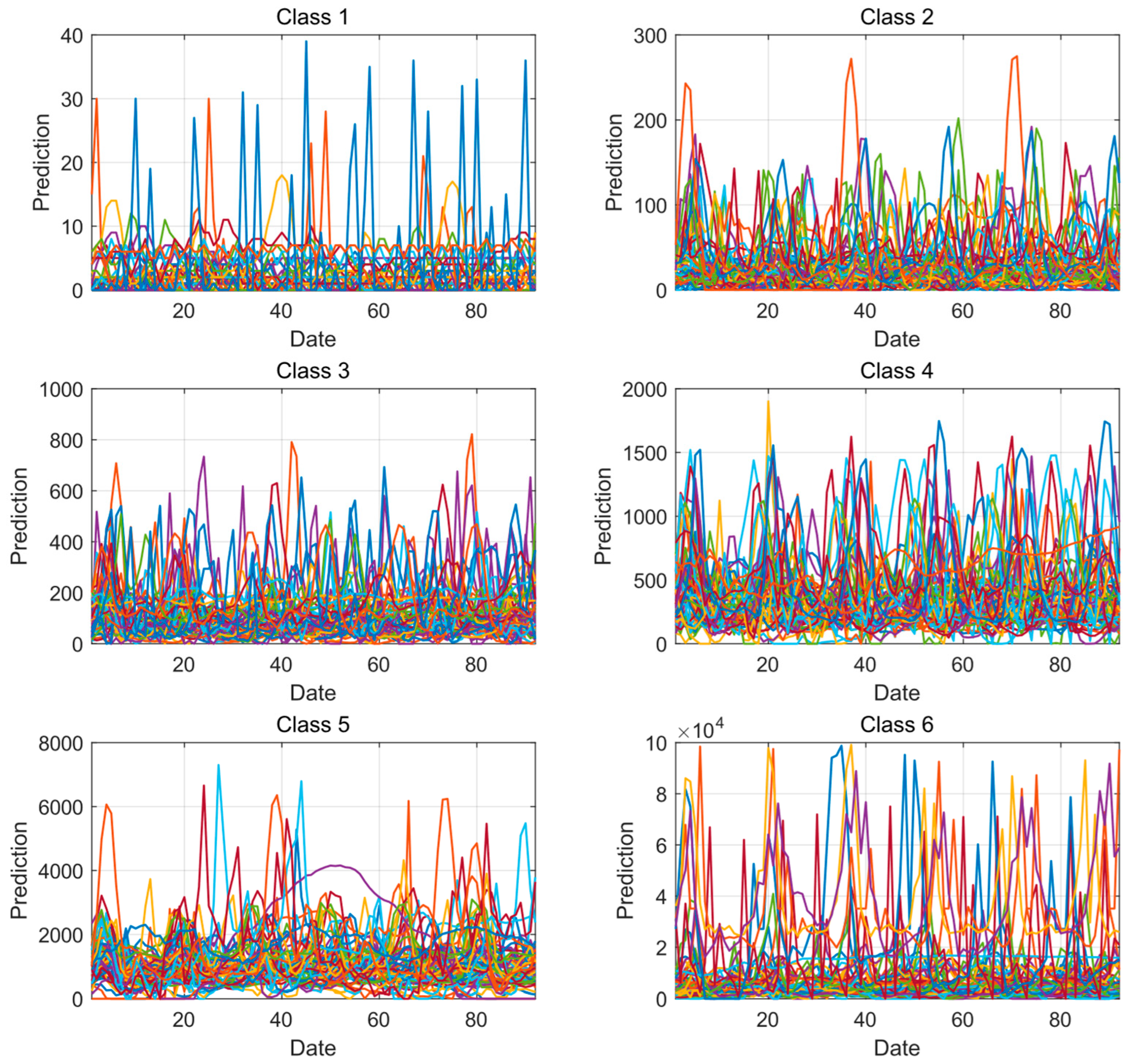
3.5. Visualization of Sales Performance Tiers

To further analyze the LSTM sales forecast results, product categories were segmented into six distinct performance tiers (Class 1 to Class 6) based on their average predicted daily sales, arranged in ascending order. This classification facilitates a more granular understanding of sales distribution and helps identify key product groups. Figure 6 visually represents this tiered structure, employing color-coding and spatial organization to offer an intuitive depiction of the sales landscape across the 350 product categories.

A detailed examination of Figure 6 reveals significant disparities in sales contributions among these performance tiers:

• High-Volume Tiers (Class 5–6): These elite categories, despite constituting only approximately 15% of the total number of product categories, are forecasted to drive a disproportionately large share of sales, accounting for roughly 30% of the total predicted sales volume. These tiers often encompass fast-moving consumer goods (FMCGs) or high-demand seasonal items, representing critical revenue drivers.
• Mid-Range Tiers (Class 3–4): This segment demonstrates moderate yet consistent sales performance. Collectively, these categories are predicted to contribute approximately 40% of the total sales volume, forming the stable core of the sales distribution.
• Low-Volume Tiers (Class 1–2): These categories are the most numerous, representing nearly 45% of all product types. However, their combined contribution to overall sales is forecasted to be relatively modest, at approximately 30%. This highlights a long-tail phenomenon, where a large number of products contribute individually small amounts to the total sales.

In Figure 6, each sales tier is represented by distinct colors to visualize the forecast distribution. Low-volume tiers (Classes 1-2) are typically shown in colors like light blue, orange, or yellow. Mid-range tiers (Classes 3-4) are represented by colors such as purple and dark green, while high-volume tiers (Classes 5-6) utilize prominent colors like dark blue and dark red.

The distinct sales distribution patterns highlighted by this visualization underscore the varying strategic importance of different product categories. Such a classification, derived from the LSTM sales forecasts, provides enterprises with actionable insights. It enables a clearer identification of three categories. (a) Key Revenue-Generating Categories (Class 5–6): These warrant prioritized attention regarding stock availability, marketing focus, and demand sensing to capitalize on their high sales potential. (b) Steady Performers (Class 3–4): These require consistent inventory management and potentially strategies for incremental sales growth. (c) Long-Tail Products (Class 1–2): For these numerous low-volume items, enterprises may need to optimize inventory strategies (e.g., consider make-to-order, centralized stocking, or rationalizing the product range) to balance availability with holding costs and avoid excessive capital tie-up. Ultimately, this visual and analytical approach empowers businesses to refine their inventory management, sales strategies, and resource allocation with greater precision.

4. Conclusions

This study addressed the critical challenge of inventory and sales forecasting within e-commerce warehousing networks by proposing and evaluating an innovative dual-model framework. We strategically employed the ARIMA algorithm for monthly inventory forecasting and the LSTM recurrent neural network for daily sales forecasting. Empirical validation demonstrated that this tailored approach yields effective predictive performance in their respective domains: ARIMA excels at capturing the trends and seasonality inherent in (differenced) stationary inventory time series, while LSTM effectively models the complex, non-linear fluctuations characteristic of daily sales data.

The forecasts generated by the proposed framework yield insights of substantial practical relevance for e-commerce operations. Specifically, they offer a robust quantitative foundation for proactive warehouse resource planning, category-specific inventory optimization, and data-driven decision making concerning site capacity and resource allocation. Collectively, these contributions have the potential to reduce holding costs, mitigate stockout risks, enhance operational efficiency, and improve overall supply chain responsiveness.

Despite these promising results, this study has certain limitations. A key constraint is the univariate nature of the forecasting models, which do not explicitly account for potential interactions and correlations between different product categories or the influence of external multivariate factors (e.g., promotional activities, competitor pricing, macroeconomic indicators). Incorporating such factors could further enhance predictive accuracy and real-world applicability.

Future research will focus on several promising directions. Firstly, we aim to explore hybrid models that more deeply integrate the strengths of ARIMA and LSTM, or other advanced time series techniques, potentially developing a unified framework capable of handling both inventory and sales data characteristics simultaneously. Secondly, a crucial next step involves investigating multivariate forecasting approaches to capture inter-dependencies between product sales and the impact of exogenous variables. This could involve Vector Autoregression (VAR) models, multivariate LSTM architectures, or models incorporating attention mechanisms to weigh the influence of different factors. Successfully addressing these areas will further refine forecasting precision and practical utility, providing even more sophisticated decision support for e-commerce operations.

References

- Huang, Z.; Ji, Q.; Chen, D. Research on intelligent logistics warehousing system in the Internet of things. Autom. Instrum. 2011, 32, 12–15. [Google Scholar]
- Wang, X.; Zhang, Q. Construction of fresh agricultural products cold chain logistics system based on Internet of things: Framework, mechanism and path. J. Nanjing Agric. Univ. (Soc. Sci. Ed.) 2016, 16, 31–41+163. [Google Scholar]
- Tulli, S.K.C. Warehouse Layout Optimization: Techniques for Improved Order Fulfillment Efficiency. Int. J. Acta Inform. 2023, 2, 138–168. [Google Scholar]
- Islam, M.R.; Ali, S.M.; Fathollahi-Fard, A.M.; Kabir, G. A novel particle swarm optimization-based grey model for the prediction of warehouse performance. J. Comput. Des. Eng. 2021, 8, 705–727. [Google Scholar] [CrossRef]
- Singh, K.; Booma, P.M.; Eaganathan, U. E-Commerce System for Sale Prediction Using Machine Learning Technique. J. Phys. Conf. Ser. 2020, 1712, 012042. [Google Scholar] [CrossRef]
- Feng, Y.; Chen, Z.; Wu, X. Smart Warehouse Management Using IoT and Big Data Analytics. IEEE Trans. Ind. Inform. 2023, 19, 4321–4332. [Google Scholar]
- Raizada, S.; Saini, J.R. Comparative analysis of supervised machine learning techniques for sales forecasting. Int. J. Adv. Comput. Sci. Appl. 2021, 12, 102–110. [Google Scholar] [CrossRef]
- Zhang, X.; He, Y.; Wang, L. Research and analysis of e-commerce sales forecasting based on integrated learning. J. Change Univ. 2024, 34, 1–7. [Google Scholar]
- Chai, F.; Zhang, L.; Su, J.; Li, F.; Gao, M.; Lv, F.; Zhang, B.; Zhan, C. Research on prediction of agricultural equipment inventory based on deep learning. Comput. Eng. Softw. 2023, 44, 21–25. [Google Scholar]
- Huang, Y.; Liang, F.; Fan, C.; Song, Z. Application of improved particle swarm optimization algorithm in inventory forecasting. J. Northwest. Polytech. Univ. 2023, 41, 428–438. [Google Scholar] [CrossRef]
- Wang, W.; Tang, R.; Li, C.; Liu, P.; Luo, L. A BP neural network model optimized by mind evolutionary algorithm for predicting the ocean wave heights. Ocean Eng. 2018, 162, 98–107. [Google Scholar] [CrossRef]
- Chafak, T.; Nur, S.; Cenk, G.; Okan, O. Short term load forecasting based on ARIMA and ANN approaches. Energy Rep. 2023, 9, 550–557. [Google Scholar]
- Tian, Z.; Yu, X.; Feng, G. Short-term wind speed prediction model based on long short-term memory network with feature extraction. Earth. Sci. Inform. 2025, 18, 333. [Google Scholar] [CrossRef]
- Gu, Y.H.; Jin, D.; Yin, H.; Zheng, R.; Piao, X.; Yoo, S.J. Forecasting agricultural commodity prices using dual input attention LSTM. Agriculture 2022, 12, 256. [Google Scholar] [CrossRef]
- Han, M.; Wang, Q. Adaptive Graph Convolution Neural Differential Equation for Spatio-Temporal Time Series Prediction. IEEE Trans. Knowl. Data Eng. 2025, 37, 3193–3204. [Google Scholar] [CrossRef]