Gene Selection Algorithms in a Single-Cell Gene Decision Space Based on Self-Information

Abstract

A critical step for gene selection algorithms using rough set theory is the establishment of a gene evaluation function to assess the classification ability of candidate gene subsets. The concept of dependency in a classic neighborhood rough set model plays the role of this evaluation function. This criterion only notes the information provided by the lower approximation and omits the upper approximation, which may result in the loss of some important information. This paper proposes gene selection algorithms within a single-cell gene decision space by employing self-information, taking into account both lower and upper approximations. Initially, the distance between gene expression values within each subspace is defined to establish the tolerance relation on the cell set. Subsequently, self-information is introduced through the lens of tolerance classes. The relationship between these measures and their respective properties is then examined in detail. For gene expression data, the proposed self-information metric demonstrates superiority over other measures by accounting for both lower and upper approximations, thereby facilitating the selection of optimal gene subsets. Finally, gene selection algorithms within a single-cell gene decision space are developed based on the proposed self-information metric, and experiments conducted on 10 publicly available single-cell datasets indicate that the classification performance of the proposed algorithms can be enhanced through the selection of genes pertinent to classification. The results demonstrate that $Fi-SI$ achieves an average classification accuracy of 93.7% (KNN) while selecting 48.3% fewer genes than Fisher’s score.

1. Introduction

1.1. Research Background

Single-cell gene expression data provide detailed molecular insights that help us better understand the functions and characteristics of cells. Through these data, we can delve into the differences between various cell types, uncover the roles of cells in disease progression and physiological processes, and provide crucial insights for personalized medicine and precision therapies. Gene selection is an effective method for understanding the factors involved in disease using single-cell gene expression data.

Rough set theory (RS-theory) is an important mathematical tool for dealing with uncertainty, inconsistency, and incomplete knowledge, and it has been used in gene selection. RS-theory constitutes a pivotal methodology for addressing uncertainty, the fundamental premise of which is the approximate quantification of inaccurate or indefinite knowledge with the known knowledge. For a classification problem, RS-theory uses attributes to induce binary relations where objects are grouped into different information granules. The decision variable is then approximately characterized by these information granules, and the lower and the upper approximations of the decision are formulated. Furthermore, a feature evaluation function, called dependency function, is defined. Different types of binary relations can lead to different rough sets such as classical rough sets, neighborhood rough sets, dominance rough sets, fuzzy rough sets [1,2], etc. An information system (IS) in the light of RS-theory, proposed by Pawlak [3], is a database that shows relationships between objects and attributes. Most applications of RS-theory are related to an IS.

Information entropy, introduced by Shannon [4], is an important tool for estimating uncertainty. Some scholars have measured the uncertainty of an IS by using information entropy. For example, Wang et al. [5] proposed a novel entropy measurement for general fuzzy relations. Zhang et al. [6] discussed uncertainty measurement in a categorical IS. Li et al. [7] investigated entropy measure of a fuzzy relation IS. Navarrete et al. [8] described an approach to smoothing RGB-D data based on information entropy. Hempelmann et al. [9] devised an evaluation method for a medical IS by using information entropy. Delgado et al. [10] raised entropy weight method-based analysis on environmental conflicts.

Feature selection is called attribute reduction in RS-theory. It is a basic data preprocessing technology in machine learning and pattern classification tasks. The aim is to eliminate redundant attributes to simplify the complexity of classification model and to improve the generalization ability of classification. To name a few, Zeng et al. [11] proposed incremental feature selection based on fuzzy rough set with Gaussian kernel; Kim et al. [12] gave a neighborhood rough set-based feature selection method; Wang et al. [13] considered attribute reduction via a fuzzy rough iterative computation model; Dai et al. [14] presented information entropy-based feature selection algorithms for an interval-valued IS; Singh et al. [15] gave feature selection approaches for set-valued data on the basis of RS-theory; Sang et al. [16] advanced incremental feature selection method via conditional entropy; Huang et al. [17] studied discernibility measure for a fuzzy $\beta$ covering IS and gave feature selection algorithms; Jia et al. [18] raised similarity-based feature selection from the viewpoint of clustering; Wang et al. [5] considered neighborhood self-information based feature selection; Li et al. [19] put forward heterogeneous feature selection via information entropy; Wang et al. [20] proposed a feature selection algorithm using local conditional entropy; Sang et al. [16] researched incremental feature selection by means of conditional entropy; Yuan et al. [21] investigated unsupervised heterogeneous feature selection based on fuzzy mutual information; Chen et al. [22] raised random sampling accelerator for attribute reduction; Jiang et al. [23] introduced accelerator for supervised attribute reduction; Chen et al. [24] presented attribute group for attribute reduction.

1.2. Related Work

Gene expression data show the abundance of gene-transcribed mRNA measured directly or indirectly in cells. The data can be used to analyze which genes have changed in expression, how genes are related to each other, and how gene activity is affected under different conditions. With the rapid developments in microarray and sequencing technology, a large amount of single-cell RNA-seq data (scRNA-seq data) has emerged [25,26]. ScRNA-seq data are important gene expression data that are required to select the correct gene from a large number of genes. Owing to technical and sampling reasons, it is difficult to identify such a gene from gene expression data with high noise, high sparsity, high dimensionality, and uncertainty. Moreover, the selection of the best genes using traditional statistical analysis and machine learning methods is often ineffective due to the uncertainty of gene expression data. Consequently, gene selection theory based on RS-theory must be established to reduce the complexity of gene expression data. For instance, Bommertet et al. [27] proposed a filter method for feature selection of high-dimensional gene expression data; Li et al. [28] researched an uncertainty measurement for scRNA-seq data using a Gaussian kernel and applied it to unsupervised gene selection; Sharma et al. [29] presented a gene selection method for cancer classification based on multi-objective meta-heuristic machine learning algorithms; and Zhang et al. [30] studied an uncertainty measurement for scRNA-seq data based on class-consistent technology and considered its applicability for semi-supervised gene selection. Entropy-based methods (Li [28] and Zhang [30]) quantify uncertainty but fail to leverage rough set granularity. Sun et al. [31] presented a joint neighborhood entropy-based gene selection method using Fisher’s score for tumor classification. While effective for class-aware feature selection, it does not distinguish between certain and possible decisions. Sheng et al. [32] introduced a feature selection method for high-dimensional single-cell gene expression data based on unsupervised learning; Zhang al. [33] considered feature selection in a neighborhood decision IS and applied it to scRNA-seq data classification; Li et al. [34] investigated gene selection in a single-cell gene decision space by means of a Gaussian kernel. The Gaussian kernel techniques model data continuity but struggle with discrete decision boundaries. Both Zhang [33] and Li [34] use dependency functions that prioritize consistent decisions, neglecting inconsistent ones. This results in information loss and suboptimal gene subsets. Zhang et al. [35] proposed a gene selection algorithm based on class-consistent technology and a fuzzy rough iterative computation model, demonstrating its effectiveness over existing methods in handling high-dimensional gene expression data. Zhang et al. [36] studied an efficient parameter optimization method based on neighborhood entropy that replaces traditional grid search by integrating neighborhood decision classes and minimizing entropy values. Ma et al. [37] proposed robust fuzzy evidence theory-based feature selection algorithms with a noise-resistant distance metric and framework for hybrid data. Yu et al. [38] introduced a fast and robust feature selection algorithm based on cross-similarity derived from a robust fuzzy relation enabling effective application to large-scale noisy gene datasets.

1.3. Motivation and Contributions

A real-valued information system (RVDIS) is one in which the information values are real numbers. If the sample, attribute, and information values in the RVDIS are the cell, gene, and gene expression values, respectively, and the gene expression data of a gene space change into scRNA-seq data, the RVDIS is then referred to as a single-cell gene decision space ($scgd$-space).

However, the above methods cannot effectively manage the uncertainty of gene expression data. Although a number of feature selection or gene selection algorithms have been proposed with rough sets, most feature evaluation functions were constructed only considering consistent decisions of objects in the lower approximation of the decision, which may lead to some information loss. In fact, classification information is not only related to the consistent decisions but is also related to the inconsistent decisions of objects in the upper approximation. The classification information of the inconsistent decisions should not be ignored in constructing a feature evaluation function.

In light of the preceding research motivations, the primary contributions of this paper encompass the following points.

(1)

Given a subspace in the $scgd$-space, the tolerance relation on the cell set is defined by introducing a variable parameter to control the distance between two gene expression values, which leads to the tolerance class. Rough approximations of this subspace are constructed. This overcomes the shortcomings of the traditional rough set model.

(2)

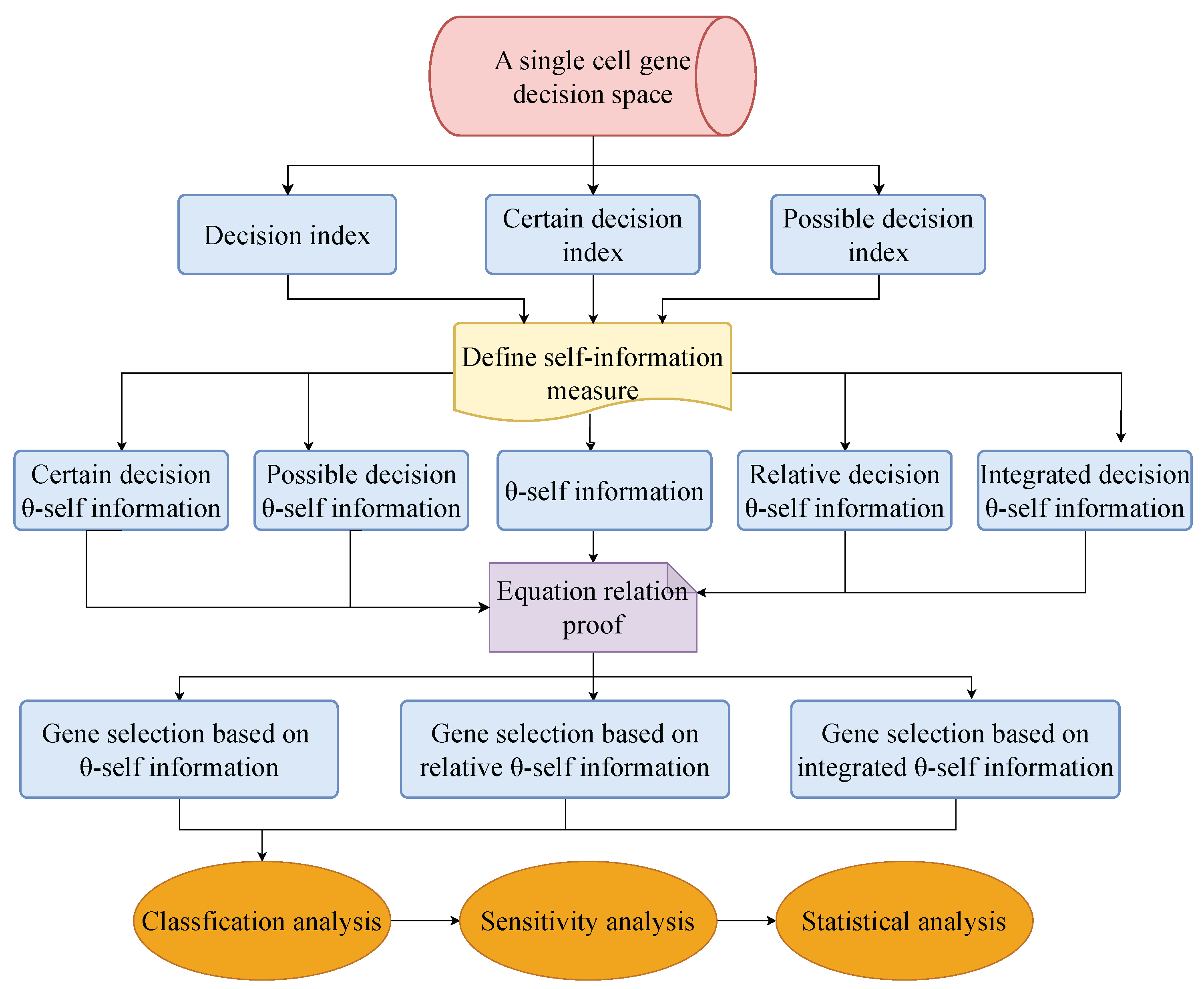
Five types of decision self-information measures as feature evaluation functions are proposed. The three feature evaluation functions with superior performance, self-information, relative self-information, and integrated self-information are chosen to design gene selection algorithms. The reason why they have superior performance is because they consider the classification information provided by both the upper and the lower approximations of the decision.

(3)

Three gene selection algorithms in an $scgd$-space are put forward using the chosen self-information. These algorithms are demonstrated in several publicly available datasets for scRNA-seq. The experimental results show that these algorithms can effectively select gene subsets and outperform the existing algorithms.

1.4. Organization and Structure

In this paper, we first analyze the shortcoming of dependency function. Then, we present three kinds of indices of uncertainty by using the lower and the upper approximations of decision: (1) decision index; (2) certain decision index; (3) possible decision index. Combined with self-information, we introduce five types of decision self-information as feature evaluation functions and obtain their related properties. Based on the self-information with the superior performance, we design three gene selection algorithms in an $scgd$-space. Finally, a series of experiments are conducted to verify that the designed algorithms can select effective gene subsets.

Figure 1 shows the flowchart for this paper.

The remainder of this article is organized as follows. Section 2 reviews rough set model on an $scgd$-space. Section 3 defines self-information in an $scgd$-space. Section 4 proposes self-information-based gene selection algorithms. Section 5 conducts numerical experiments to demonstrate the performance of the proposed algorithms. Section 6 summarizes this paper.

2. A Single-Cell Gene Decision Space and Rough Set Model

This part reviews the single-cell gene decision space and considers the rough set model in an $scgd$-space.

In this paper, S, $2^S$, and $\left|W\right|$ represent a finite set, the family of all subsets of S, and the cardinality of $W\in 2^S$, respectively. Put

$$S=\{s_1,s_2,\dots ,s_n\}.$$

(1)

$(S,C,d)$ is known as a real-valued decision information system (RVDIS), if $\forall a\in C$, $\forall s\in S$, $a\left(s\right)$ is a real number, where C is the conditional attribute set and d is a decision attribute.

Definition 1

([34]). For a RVDIS $(S,C,d)$, suppose that S and C are the sets of cells and genes to describe the cells, respectively. If $\forall a\in C,s\in S$, $a\left(s\right)$ expresses the gene expression value of the cell s relative to the gene a and the gene expression data in $(S,C,d)$ are single cell RNA-seq data (scRNA-seq data), then $(S,C,d)$ is known as a single-cell gene decision space ($scgd$-space).

Definition 2

([34]). For an $scgd$-space $(S,C,d)$, $\forall a\in C$, $\forall s,s^{\prime }\in S$, the distance between $a\left(s\right)$ and $a\left(s^{\prime }\right)$ is known as

$$dis(a\left(s\right),a\left(s^{\prime }\right))={\displaystyle \frac{|a\left(s\right)-a\left(s^{\prime }\right)|}{max\left\{a\right(x):x\in S\}-min\left\{a\right(x):x\in S\}}}.$$

(2)

Definition 3.

For an $scgd$-space $(S,C,d)$, let $G\subseteq C$ and $\theta \in [0,1]$, put

$$G^{\theta }=\{(s,s^{\prime })\in S\times S:\forall a\in G,dis(a\left(s\right),a\left(s^{\prime }\right))\le \theta \},$$

(3)

$$R_d=\{(s,s^{\prime })\in S\times S:d\left(s\right)=d\left(s^{\prime }\right)\}.$$

(4)

Clearly, $G^{\theta }$ and $R_d$ are tolerance (reflexive and symmetric) and equivalence relations on S, respectively.

Denote

$$a^{\theta }={\left\{a\right\}}^{\theta }.$$

Put

$$G^{\theta }\left(s\right)=\{s^{\prime }\in S:(s,s^{\prime })\in G^{\theta }\},$$

(5)

$$R_d\left(s\right)=\{s^{\prime }\in S:(s,s^{\prime })\in R_d\}.$$

(6)

Then, $G^{\theta }\left(s\right)$ and $R_d\left(s\right)$ are known as the tolerance and decision classes of o, respectively.

Denote

$$S/R_d=\{R_d\left(s\right):s\in S\}=\{{\mathbb{D}}_1,{\mathbb{D}}_2,\dots ,{\mathbb{D}}_r\}.$$

(7)

Proposition 1.

For an $scgd$-space $(S,C,d)$.

(1) 

If $G_1\subseteq G_2$, then $\forall \theta \in [0,1]$, $\forall s\in S$, ${G_2}^{\theta }\left(s\right)\subseteq {G_1}^{\theta }\left(s\right);$

(2) 

If $0\le {\theta }_1\le {\theta }_2\le 1$, then $\forall G\subseteq C$, $\forall s\in S$, $G^{{\theta }_1}\left(s\right)\subseteq G^{{\theta }_2}\left(s\right).$

Proof. 

Obviously.    □

Definition 4.

For an $scgd$-space $(S,C,d)$, let $G\subseteq C$ and $\theta \in [0,1]$. Define ${\partial }_G^{\theta }:S\to 2^{V_d}$ as follows:

$${\partial }_G\left(s\right)=d\left(G^{\theta }\left(s\right)\right).$$

(8)

Then, ${\partial }_G^{\theta }$ is known as generalized decision in $(S,G,d)$.

If $\forall s\in S$, $|{\partial }_C^{\theta }\left(s\right)|=1$, then $(S,C,d)$ is known as θ-consistent; otherwise, it is known as θ-inconsistent.

Proposition 2.

Let $(S,C,d)$ be an $scgd$-space. Given $G\subseteq C$ and $\theta \in [0,1]$. Then,

$$G^{\theta }\subseteq R_d\iff \forall s\in S,\left|{\partial }_G^{\theta }\left(s\right)\right|=1.$$

(9)

Proof. 

$“\Rightarrow ”$. Let $G^{\theta }\subseteq R_d$. Then, $\forall s\in S,G^{\theta }\left(s\right)\subseteq R_d\left(s\right)$. Suppose $t\in {\partial }_G^{\theta }\left(s\right)$. Then, $t=d\left(s^{\prime }\right)$ for some $s^{\prime }\in G^{\theta }\left(s\right)$. $s^{\prime }\in G^{\theta }\left(s\right)$ implies that $s^{\prime }\in R_d\left(s\right)$. So, $t=d\left(s^{\prime }\right)=d\left(s\right)$. Thus, $\forall s\in S,|{\partial }_G^{\theta }\left(s\right)|=1.$

$“\Leftarrow ”$. Assume that $\forall s\in S,|{\partial }_G^{\theta }\left(s\right)|=1$. Suppose $s^{\prime }\in G^{\theta }\left(s\right)$. Then, $d\left(s^{\prime }\right)\in {\partial }_G^{\theta }\left(s\right)$. Since $d\left(s\right)\in {\partial }_G^{\theta }\left(s\right)$ and $|{\partial }_G^{\theta }\left(s\right)|=1$, we have $d\left(s\right)=d\left(s^{\prime }\right)$. Then, $s^{\prime }\in R_d\left(s\right)$. Thus, $G^{\theta }\left(s\right)\subseteq R_d\left(s\right)$.    □

Theorem 1.

Let $(S,C,d)$ be an $scgd$-space. Given $\theta \in [0,1]$. Then, $(S,C,d)$ is θ-consistent ⇔ $C^{\theta }\subseteq R_d.$

Proof. 

It can be proven using Proposition 2.    □

Define

$$\underline{G^{\theta }}\left(W\right)=\{s\in S:G^{\theta }\left(s\right)\subseteq W\},$$

(10)

$$\overline{G^{\theta }}\left(W\right)=\{s\in S:G^{\theta }\left(s\right)\cap W\ne \varnothing \}.$$

(11)

Proposition 3.

For an $scgd$-space $(S,C,d)$.

(1) 

If $W_1\subseteq W_2\subseteq S$, then $\forall G\subseteq C$, $\forall \theta \in [0,1]$,

$$\underline{G^{\theta }}\left(W_1\right)\subseteq \underline{G^{\theta }}\left(W_2\right),\overline{G^{\theta }}\left(W_1\right)\subseteq \overline{G^{\theta }}\left(W_2\right);$$

(2) 

If $G_1\subseteq G_2\subseteq C$, then $\forall \theta \in [0,1]$, $\forall W\in 2^S$

$$\underline{{G_1}^{\theta }}\left(W\right)\subseteq \underline{{G_2}^{\theta }}\left(W\right),\overline{{G_2}^{\theta }}\left(W\right)\subseteq \overline{{G_1}^{\theta }}\left(W\right);$$

(3) 

If $0\le {\theta }_1\le {\theta }_2\le 1$, then $\forall G\subseteq C$, $\forall W\in 2^S$,

$${\underline{R}}_G^{{\theta }_2}\left(W\right)\subseteq {\underline{R}}_G^{{\theta }_1}\left(W\right),{\overline{R}}_G^{{\theta }_1}\left(W\right)\subseteq {\overline{R}}_G^{{\theta }_2}\left(W\right).$$

Proof. 

It can be proven using Proposition 1.    □

3. Self-Information of a Subspace in an $\mathit{scgd}$-Space

Definition 5

([4]). Let x be a random variable. $p\left(x\right)$ denotes the probability of x. Suppose that $I\left(x\right)$ is a metric of the uncertainty of x. Then, $I\left(x\right)$ is known as the self-information of x if meets the following conditions:

(1) 

Non-negative: $I\left(x\right)\ge 0$;

(2) 

If $p\left(x\right)\to 0$, then $I\left(x\right)\to \infty$;

(3) 

If $p\left(x\right)=1$, then $I\left(x\right)=0$.

(4) 

Strict monotonic: If $p\left(x\right)>p\left(y\right)$, then $I\left(x\right)<I\left(y\right)$.

Let $(S,C,d)$ be an $scgd$-space. Given $G\subseteq C$ and $\theta \in [0,1]$.

(1)

$\theta$-positive region of G with respect to d is known as

$$PO{S}_G^{\theta }\left(d\right)=\bigcup _{i=1}^r\underline{G}\left({\mathbb{D}}_i\right);$$

(12)

(2)

$\theta$-dependence of G with respect to d is known as

$${\mathsf{\Gamma }}_G^{\theta }\left(d\right)={\displaystyle \frac{1}{n}}\left|PO{S}_G^{\theta }\left(d\right)\right|.$$

(13)

${\mathsf{\Gamma }}_G^{\theta }\left(d\right)$ can be used as the criterion for gene selection. However, it only notes consistent cells in the lower approximation and ignores inconsistent cells that have important classification information. Inconsistent cells may be merged in the upper approximation. Thus, the criterion for gene selection should contain both the lower and the upper approximations of the decision.

Let $(S,C,d)$ be an $scgd$-space. Given $G\subseteq C$ and $\theta \in [0,1]$. $\forall i$, define

$$dec\left({\mathbb{D}}_i\right)=|{\mathbb{D}}_i|,cer{t}_G^{\theta }\left({\mathbb{D}}_i\right)=|\underline{G^{\theta }}\left({\mathbb{D}}_i\right)|,pos{s}_G^{\theta }\left({\mathbb{D}}_i\right)=\left|\overline{G^{\theta }}\left({\mathbb{D}}_i\right)\right|.$$

(14)

Then, $dec\left({\mathbb{D}}_i\right)$, $cer{t}_G^{\theta }\left({\mathbb{D}}_i\right)$ and $pos{s}_G^{\theta }\left({\mathbb{D}}_i\right)$ are called the decision index, certain decision index, and possible decision index of ${\mathbb{D}}_i$, respectively,

Due to the properties that the metric has, combined with self-information, the following definition is introduced.

Definition 6.

For an $scgd$-space $(S,C,d)$, let $G\subseteq C$ and $\theta \in [0,1]$, define

$$\mathrm{c}-S{I}_G^{\theta }\left(d\right)=-\sum _{i=1}^r(1-{\displaystyle \frac{cer{t}_G^{\theta }\left({\mathbb{D}}_i\right)}{dec\left({\mathbb{D}}_i\right)}})lo{g}_2{\displaystyle \frac{cer{t}_G^{\theta }\left({\mathbb{D}}_i\right)}{dec\left({\mathbb{D}}_i\right)}};$$

(15)

$$\mathrm{p}-S{I}_G^{\theta }\left(d\right)=-\sum _{i=1}^r(1-{\displaystyle \frac{dec\left({\mathbb{D}}_i\right)}{pos{s}_G^{\theta }\left({\mathbb{D}}_i\right)}})lo{g}_2{\displaystyle \frac{dec\left({\mathbb{D}}_i\right)}{pos{s}_G^{\theta }\left({\mathbb{D}}_i\right)}};$$

(16)

$$S{I}_G^{\theta }\left(d\right)={\displaystyle \frac{1}{2}}(\mathrm{c}-S{I}_G^{\theta }\left(d\right)+\mathrm{p}-S{I}_G^{\theta }\left(d\right));$$

(17)

$$\mathrm{r}-S{I}_G^{\theta }\left(d\right)=-\sum _{i=1}^r(1-{\displaystyle \frac{cer{t}_G^{\theta }\left({\mathbb{D}}_i\right)}{pos{s}_G^{\theta }\left({\mathbb{D}}_i\right)}})lo{g}_2{\displaystyle \frac{cer{t}_G^{\theta }\left({\mathbb{D}}_i\right)}{pos{s}_G^{\theta }\left({\mathbb{D}}_i\right)}}.$$

(18)

Then, $cd$-$S{I}_G^{\theta }\left(d\right)$, $pd$-$S{I}_G^{\theta }\left(d\right)$, $S{I}_G^{\theta }\left(d\right)$ and r-$S{I}_G^{\theta }\left(d\right)$ are called the certain decision θ-self information, possible decision θ-self-information, θ-self-information and relative θ-self-information of the subspace $(S,G,d)$, respectively.

When $G=\varnothing$, let

$$c-S{I}_G^{\theta }\left(d\right)=p-S{I}_G^{\theta }\left(d\right)=S{I}_G^{\theta }\left(d\right)=r-S{I}_G^{\theta }\left(d\right)=-\sum _{i=1}^r(1-{\displaystyle \frac{de{c}^{\theta }\left({\mathbb{D}}_i\right)}{n}})lo{g}_2{\displaystyle \frac{de{c}^{\theta }\left({\mathbb{D}}_i\right)}{n}}.$$

Four kinds of decision self-information measures in Definition 6 characterize the classification ability of feature subset G from different angles, respectively. Thus, they can be viewed as feature evaluation functions.

Proposition 4.

For an $scgd$-space $(S,C,d)$.

(1) 

If $G_1\subseteq G_2\subseteq C$, then

$$\mathrm{c}-S{I}_{G_2}^{\theta }\left(d\right)\le \mathrm{c}-S{I}_{G_1}^{\theta }\left(d\right),\mathrm{p}-S{I}_{G_2}^{\theta }\left(d\right)\le \mathrm{p}-S{I}_{G_1}^{\theta }\left(d\right),$$

$$S{I}_{G_2}^{\theta }\left(d\right)\le S{I}_{G_1}^{\theta }\left(d\right),\mathrm{r}-S{I}_{G_2}^{\theta }\left(d\right)\le \mathrm{r}-S{I}_{G_1}^{\theta }\left(d\right).$$

(2) 

If $0\le {\theta }_1\le {\theta }_2\le 1$, then

$$\mathrm{c}-S{I}_G^{{\theta }_1}\left(d\right)\le \mathrm{c}-S{I}_G^{{\theta }_2}\left(d\right),\mathrm{p}-S{I}_G^{{\theta }_1}\left(d\right)\le \mathrm{p}-S{I}_G^{{\theta }_2}\left(d\right),$$

$$S{I}_G^{{\theta }_1}\left(d\right)\le S{I}_G^{{\theta }_2}\left(d\right),\mathrm{r}-S{I}_G^{{\theta }_1}\left(d\right)\le \mathrm{r}-S{I}_G^{{\theta }_2}\left(d\right).$$

(3) 

$$2S{I}_G^{\theta }\left(d\right)\le \mathrm{r}-S{I}_G^{\theta }\left(d\right).$$

Proof. 

(1) Suppose $G_1\subseteq G_2\subseteq C$. Then, from Proposition 3(2), we have

$$\forall i,\underline{{G_1}^{\theta }}\left({\mathbb{D}}_i\right)\subseteq \underline{{G_2}^{\theta }}\left({\mathbb{D}}_i\right).$$

So, $\forall i$, $cer{t}_{G_1}^{\theta }\left({\mathbb{D}}_i\right)\le cer{t}_{G_2}^{\theta }\left({\mathbb{D}}_i\right).$ It follows that $\forall i$,

$${\displaystyle \frac{cer{t}_{G_1}^{\theta }\left({\mathbb{D}}_i\right)}{dec\left({\mathbb{D}}_i\right)}}\le {\displaystyle \frac{cer{t}_{G_2}^{\theta }\left({\mathbb{D}}_i\right)}{dec\left({\mathbb{D}}_i\right)}},lo{g}_2{\displaystyle \frac{cer{t}_{G_1}^{\theta }\left({\mathbb{D}}_i\right)}{dec\left({\mathbb{D}}_i\right)}}\le lo{g}_2{\displaystyle \frac{cer{t}_{G_2}^{\theta }\left({\mathbb{D}}_i\right)}{dec\left({\mathbb{D}}_i\right)}}.$$

Thus,

$$0\le 1-{\displaystyle \frac{cer{t}_{G_2}^{\theta }\left({\mathbb{D}}_i\right)}{dec\left({\mathbb{D}}_i\right)}}\le 1-{\displaystyle \frac{cer{t}_{G_1}^{\theta }\left({\mathbb{D}}_i\right)}{dec\left({\mathbb{D}}_i\right)}},0\le -lo{g}_2{\displaystyle \frac{cer{t}_{G_2}^{\theta }\left({\mathbb{D}}_i\right)}{dec\left({\mathbb{D}}_i\right)}}\le -lo{g}_2{\displaystyle \frac{cer{t}_{G_1}^{\theta }\left({\mathbb{D}}_i\right)}{dec\left({\mathbb{D}}_i\right)}}.$$

Hence,

$$c-S{I}_{G_2}^{\theta }\left(d\right)\le c-S{I}_{G_1}^{\theta }\left(d\right).$$

Similarly, we can prove that

$$G_1\subseteq G_2\Rightarrow p-S{I}_{G_2}^{\theta }\left(d\right)\le p-S{I}_{G_1}^{\theta }\left(d\right),S{I}_{G_2}^{\theta }\left(d\right)\le S{I}_{G_1}^{\theta }\left(d\right),r-S{I}_{G_2}^{\theta }\left(d\right)\le r-S{I}_{G_1}^{\theta }\left(d\right).$$

(2) Suppose $0\le {\theta }_1\le {\theta }_2\le 1$. Then, from Proposition 3(3), we have

$$\forall i,{\underline{R}}_G^{{\theta }_2}\left({\mathbb{D}}_i\right)\subseteq {\underline{R}}_G^{{\theta }_1}\left({\mathbb{D}}_i\right).$$

So, $\forall i$, $cer{t}_G^{{\theta }_2}\left({\mathbb{D}}_i\right)\le cer{t}_G^{{\theta }_1}\left({\mathbb{D}}_i\right).$ It follows that $\forall i$,

$${\displaystyle \frac{cer{t}_G^{{\theta }_2}\left({\mathbb{D}}_i\right)}{dec\left({\mathbb{D}}_i\right)}}\le {\displaystyle \frac{cer{t}_G^{{\theta }_1}\left({\mathbb{D}}_i\right)}{dec\left({\mathbb{D}}_i\right)}},lo{g}_2{\displaystyle \frac{cer{t}_G^{{\theta }_2}\left({\mathbb{D}}_i\right)}{dec\left({\mathbb{D}}_i\right)}}\le lo{g}_2{\displaystyle \frac{cer{t}_G^{{\theta }_1}\left({\mathbb{D}}_i\right)}{dec\left({\mathbb{D}}_i\right)}}.$$

Thus,

$$0\le 1-{\displaystyle \frac{cer{t}_G^{{\theta }_1}\left({\mathbb{D}}_i\right)}{dec\left({\mathbb{D}}_i\right)}}\le 1-{\displaystyle \frac{cer{t}_G^{{\theta }_2}\left({\mathbb{D}}_i\right)}{dec\left({\mathbb{D}}_i\right)}},0\le -lo{g}_2{\displaystyle \frac{cer{t}_G^{{\theta }_1}\left({\mathbb{D}}_i\right)}{dec\left({\mathbb{D}}_i\right)}}\le -lo{g}_2{\displaystyle \frac{cer{t}_G^{{\theta }_2}\left({\mathbb{D}}_i\right)}{dec\left({\mathbb{D}}_i\right)}}.$$

Hence,

$$c-S{I}_G^{{\theta }_1}\left(d\right)\le c-S{I}_G^{{\theta }_2}\left(d\right).$$

Similarly, we can prove that

$${\theta }_1\le {\theta }_2\Rightarrow p-S{I}_G^{{\theta }_1}\left(d\right)\le p-S{I}_G^{{\theta }_2}\left(d\right),S{I}_G^{{\theta }_1}\left(d\right)\le S{I}_G^{{\theta }_2}\left(d\right),r-S{I}_G^{{\theta }_1}\left(d\right)\le r-S{I}_G^{{\theta }_2}\left(d\right).$$

(3) Put

$$m_i^{\left(1\right)}={\displaystyle \frac{cer{t}_G^{{\theta }_1}\left({\mathbb{D}}_i\right)}{dec\left({\mathbb{D}}_i\right)}},m_i^{\left(2\right)}={\displaystyle \frac{dec\left({\mathbb{D}}_i\right)}{pos{s}_G^{{\theta }_1}\left({\mathbb{D}}_i\right)}},m_i^{\left(3\right)}={\displaystyle \frac{cer{t}_G^{{\theta }_1}\left({\mathbb{D}}_i\right)}{pos{s}_G^{{\theta }_1}\left({\mathbb{D}}_i\right)}};$$

$$n_i^{\left(1\right)}=1-m_i^{\left(1\right)},n_i^{\left(2\right)}=1-m_i^{\left(2\right)},n_i^{\left(3\right)}=1-m_i^{\left(3\right)}.$$

Then, $m_i^{\left(3\right)}=m_i^{\left(1\right)}{m}_i^{\left(2\right)}$ and

$$n_i^{\left(3\right)}=1-m_i^{\left(1\right)}{m}_i^{\left(2\right)}=1-(1-n_i^{\left(1\right)})(1-n_i^{\left(2\right)})=n_i^{\left(1\right)}+n_i^{\left(2\right)}-n_i^{\left(1\right)}{n}_i^{\left(2\right)}.$$

$$\begin{array}{cc}\hfill r-S{I}_G^{\theta }\left(d\right)& =-\sum _{i=1}^r{n}_i^{\left(3\right)}lo{g}_2{m}_i^{\left(3\right)}=-\sum _{i=1}^r{n}_i^{\left(3\right)}lo{g}_2\left(m_i^{\left(1\right)}{m}_i^{\left(2\right)}\right)\hfill \\ \hfill & =-\sum _{i=1}^r{n}_i^{\left(3\right)}lo{g}_2{m}_i^{\left(1\right)}-\sum _{i=1}^r{n}_i^{\left(3\right)}lo{g}_2{m}_i^{\left(2\right)}\hfill \\ \hfill & =-\sum _{i=1}^r{n}_i^{\left(1\right)}lo{g}_2{m}_i^{\left(1\right)}-\sum _{i=1}^r{n}_i^{\left(2\right)}lo{g}_2{m}_i^{\left(2\right)}+\epsilon \hfill \\ \hfill & =c-S{I}_G^{\theta }\left(d\right)+p-S{I}_G^{\theta }\left(d\right)+\epsilon \hfill \\ \hfill & =2S{I}_G^{\theta }\left(d\right)+\epsilon .\hfill \end{array}$$

$$\begin{array}{cc}\hfill \epsilon & =-\sum _{i=1}^r{n}_i^{\left(3\right)}lo{g}_2{m}_i^{\left(1\right)}-\sum _{i=1}^r{n}_i^{\left(3\right)}lo{g}_2{m}_i^{\left(2\right)}+\sum _{i=1}^r{n}_i^{\left(1\right)}lo{g}_2{m}_i^{\left(1\right)}+\sum _{i=1}^r{n}_i^{\left(2\right)}lo{g}_2{m}_i^{\left(2\right)}\hfill \\ \hfill & =-\sum _{i=1}^r(n_i^{\left(3\right)}-n_i^{\left(1\right)})lo{g}_2{m}_i^{\left(1\right)}-\sum _{i=1}^r(n_i^{\left(3\right)}-n_i^{\left(2\right)})lo{g}_2{m}_i^{\left(2\right)}\hfill \\ \hfill & =-\sum _{i=1}^r(n_i^{\left(2\right)}-n_i^{\left(1\right)}{n}_i^{\left(2\right)})lo{g}_2{m}_i^{\left(1\right)}-\sum _{i=1}^r(n_i^{\left(1\right)}-n_i^{\left(1\right)}{n}_i^{\left(2\right)})lo{g}_2{m}_i^{\left(2\right)}\hfill \\ \hfill & =-\sum _{i=1}^r{n}_i^{\left(2\right)}(1-n_i^{\left(1\right)})lo{g}_2{m}_i^{\left(1\right)}-\sum _{i=1}^r{n}_i^{\left(1\right)}(1-n_i^{\left(2\right)})lo{g}_2{m}_i^{\left(2\right)}\hfill \\ \hfill & \ge 0.\hfill \end{array}$$

Thus, $2S{I}_G^{\theta }\left(d\right)\le r-S{I}_G^{\theta }\left(d\right)$.    □

Definition 7.

For a $scgd$-space $(S,C,d)$, let $G\subseteq C$ and $\theta ,\alpha \in [0,1]$, define

$$\mathrm{i}-S{I}_G^{\theta ,\alpha }\left(d\right)=\alpha S{I}_G^{\theta }\left(d\right)+(1-\alpha )\mathrm{p}-S{I}_G^{\theta }\left(d\right),$$

(19)

where α and $1-\alpha$ are the weighting factors of $S{I}_G^{\theta }\left(d\right)$ and $\mathrm{p}-S{I}_G^{\theta }\left(d\right)$, respectively. Then, $\mathrm{i}-S{I}_G^{\theta ,\alpha }\left(d\right)$ is called integrated θ-self-information of the subspace $(S,G,d)$ with respect to α.

Example 1.

For a $scgd$-space $(S,C,d)$ listed in

Table 1. Decision table.

	${\mathit{a}}_1$	${\mathit{a}}_2$	${\mathit{a}}_3$	d
$x_1$	0	0	0.1429	1
$x_1$	0.2857	1.0000	1.0000	1
$x_1$	1.0000	0.2500	0	0

, where $S=\{x_1,x_2,x_3\}$ is a set of cells, $C=\{a_1,a_2,a_3\}$ is a set of genes, and d is a decision attribute that divides the domain S into two decision equivalence classes ${\mathbb{D}}_1=\{x_1,x_2\}$ and ${\mathbb{D}}_2=\left\{x_3\right\}$.

If the neighborhood granule size is set at $\theta =0.3$, the relation matrices are listed as follows:

$$G_{a_1}^{\theta }=\left(\begin{array}{ccc}1& 1& 0\\ 1& 1& 0\\ 0& 0& 1\end{array}\right),G_{a_2}^{\theta }=\left(\begin{array}{ccc}1& 0& 1\\ 0& 1& 0\\ 1& 0& 1\end{array}\right),G_{a_3}^{\theta }=\left(\begin{array}{ccc}1& 0& 1\\ 0& 1& 0\\ 1& 0& 1\end{array}\right),$$

and the certain decision index and the possible decision index are listed in

Table 2. Certain decision index.

$\mathit{S}/\mathit{d}$	${\mathbb{D}}_1$	${\mathbb{D}}_2$
$cer{t}_{a_1}^{\theta }\left({\mathbb{D}}_k\right)$	1	2
$cer{t}_{a_2}^{\theta }\left({\mathbb{D}}_k\right)$	0	1
$cer{t}_{a_3}^{\theta }\left({\mathbb{D}}_k\right)$	0	1

and

Table 3. Possible decision index.

$\mathit{S}/\mathit{d}$	${\mathbb{D}}_1$	${\mathbb{D}}_2$
$pos{s}_{a_1}^{\theta }\left({\mathbb{D}}_k\right)$	1	2
$pos{s}_{a_2}^{\theta }\left({\mathbb{D}}_k\right)$	2	3
$pos{s}_{a_3}^{\theta }\left({\mathbb{D}}_k\right)$	2	3

, respectively.

Then, the decision self-information is listed in

Table 4. Decision self-information of ${\mathbb{D}}_i$.

B	$\mathit{c}\text{-}{\mathit{SI}}_{\mathit{B}}^{\mathit{\theta }}\left({\mathbb{D}}_1\right)$	$\mathit{p}\text{-}{\mathit{SI}}_{\mathit{B}}^{\mathit{\theta }}\left({\mathbb{D}}_1\right)$	${\mathit{SI}}_{\mathit{B}}^{\mathit{\theta }}\left({\mathbb{D}}_1\right)$	$\mathit{r}\text{-}{\mathit{SI}}_{\mathit{B}}^{\mathit{\theta }}\left({\mathbb{D}}_1\right)$	$\mathit{i}\text{-}{\mathit{SI}}_{\mathit{B}}^{\mathit{\theta }}\left({\mathbb{D}}_1\right)$	$\mathit{c}\text{-}{\mathit{SI}}_{\mathit{B}}^{\mathit{\theta }}\left({\mathbb{D}}_2\right)$	$\mathit{p}\text{-}{\mathit{SI}}_{\mathit{B}}^{\mathit{\theta }}\left({\mathbb{D}}_2\right)$	${\mathit{SI}}_{\mathit{B}}^{\mathit{\theta }}\left({\mathbb{D}}_2\right)$	$\mathit{r}\text{-}{\mathit{SI}}_{\mathit{B}}^{\mathit{\theta }}\left({\mathbb{D}}_2\right)$	$\mathit{i}\text{-}{\mathit{SI}}_{\mathit{B}}^{\mathit{\theta }}\left({\mathbb{D}}_2\right)$
$a_1$	0	0	0	0	0	0	0	0	0	0
$a_2$	0	0.3466	0.1733	0.3466	0.2426	0.3466	0.1352	0.2409	0.7324	0.1986
$a_3$	0	0.3466	0.1733	0.3466	0.2426	0.3466	0.1352	0.2409	0.7324	0.1986

and

Table 5. Decision self-information.

B	$\mathit{c}\text{-}{\mathit{SI}}_{\mathit{B}}^{\mathit{\theta }}\left(\mathit{d}\right)$	$\mathit{p}\text{-}{\mathit{SI}}_{\mathit{B}}^{\mathit{\theta }}\left(\mathit{d}\right)$	${\mathit{SI}}_{\mathit{B}}^{\mathit{\theta }}\left(\mathit{d}\right)$	$\mathit{r}\text{-}{\mathit{SI}}_{\mathit{B}}^{\mathit{\theta }}\left(\mathit{d}\right)$	$\mathit{i}\text{-}{\mathit{SI}}_{\mathit{B}}^{\mathit{\theta }}\left(\mathit{d}\right)$
$a_1$	0	0	0	0	0
$a_2$	0.3466	0.4818	0.4142	1.0808	0.4412
$a_3$	0.3466	0.4818	0.4142	1.0808	0.4412

.

4. Gene Selection Algorithms in an $\mathit{scgd}$-Space Based on Self-Information

4.1. Preliminaries

Definition 8.

For an $scgd$-space $(S,C,d)$, the normalization equation of an $scgd$-space is known as

$$x_{ij}^{*}={\displaystyle \frac{x_{ij}-x_j^{min}}{(x_j^{max}-x_j^{min})+\tau }}.$$

(20)

where $x_{ij}$ denotes the gene expression level of the $x_i$ versus the gene $a_j$, $x_j^{max}=max\left\{x_{ij}:i=1,2,\dots ,n\right\}$, $x_j^{min}=min\left\{x_{ij}:i=1,2,\dots ,n\right\}$, to avoid the overflow error when denominator equals 0, the parameter τ denotes a very small number.

A preliminary subset of genes from an $scgd$-space is selected using Fisher’s score.

Definition 9.

Let (S,C,d) be an $scgd$-space and gene $a\in C$. Fisher’s score $f\left(a\right)$ of a is formulated as

$$f\left(a\right)={\displaystyle \frac{{\sum }_{j=1}^n{m}_j{\left({\mu }_j^a-{\mu }^a\right)}^2}{\left({\sum }_{j=1}^n{m}_j{\left({\theta }_j^a\right)}^2\right)+\tau }}.$$

(21)

in which n stand for the number of ground truth classes, $m_j$ stand for the number of cells of class j, ${\mu }_j^a$ and ${\theta }_j^a$ denote the average value and standard deviation of cells of class j in terms of gene a, ${\mu }^a$ represents the average value of all cells in terms of gene a. Since some scRNA-seq data may contain values that all ${\theta }_j^a$ are equal to zero, τ is a very small number used to prevent zeros from appearing in the denominator.

Based on Fisher’s score defined in Formula (21), we propose algorithm for selection preliminary subset of genes.

Let k be the number of genes that expected. In Algorithm 1, Fisher’s score is used as measure to select genes according to Definition 9.

Algorithm 1 has a “for” loop that determines its time complexity. Given that $\left|S\right|=n$ and $\left|C\right|=m$, Algorithm 1 has a time complexity of $O\left(m\right)$. This means that the time taken by Algorithm 1 to execute increases linearly with the size of C and not S.

Algorithm 1: An algorithm for selecting genes in an $scgd$-space based on Fisher’s score

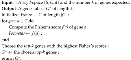
4.2. Gene Selection Algorithms

Based on $\theta$-self-information, relative $\theta$-self-information, and integrated $\theta$-self-information, we propose three gene selection algorithms (i.e., Algorithms 2–4) in an $scgd$-space. To reduce the time complexities of the three algorithms, Algorithm 1 is preliminarily employed to select a gene subset. Afterwards, the proposed algorithms are applied to the gene subsets above to select a core gene subset. With the preprocessing step, the proposed algorithms input a much smaller gene subset compared to the original gene set and have a greatly reduced time complexity.

Considering that $\theta$-self-information and relative $\theta$-self-information cannot only combine the classification information of upper and lower approximations and reduce the possibility of misclassification but also have a better convergence effect, we choose them as a feature evaluation functions to measure the classification ability of a feature subset. Based on this reason, we propose the following algorithms (i.e., Algorithms 2 and 3).

Integrated $\theta$-self-information not only has the same efficacy as $\theta$-self-information and relative $\theta$-self-information, but also uses their weights when utilizing the efficacy of $\theta$-self-information and relative $\theta$-self-information. Based on this reason, we propose Algorithm 4.

Given that $\left|S\right|=n$, $\left|C\right|=m$, $\left|G^{*}\right|=m_{G^{*}}$. The “while” loop on the outer side and the “for” loop on the inner side of Algorithm 2 determine its time complexity. Due to the variable start determining the outer “while” loop, the intersection of all elements in $G^{*}$ must be calculated in the worst case. So, Algorithm 2 has a best time complexity of $O\left(n^2{m}_{G^{*}}\right)$ and a worst time complexity of $O\left(n^2{m}_{G^{*}}^2\right)$. Similarly, Algorithms 3 and 4 also have an approximate time complexity of $O\left(n^2{m}_{G^{*}}^2\right)$. In particular, since $m_{G^{*}}\ll m$, the result of Algorithm 1 has a large impact on the time complexity of the proposed algorithms. Figure 2 shows the framework charts of Algorithm 4.

Algorithm 2: A gene selection algorithm based on $\theta$-self-information (F-$SI$) in an $scgd$-space

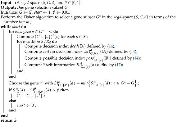
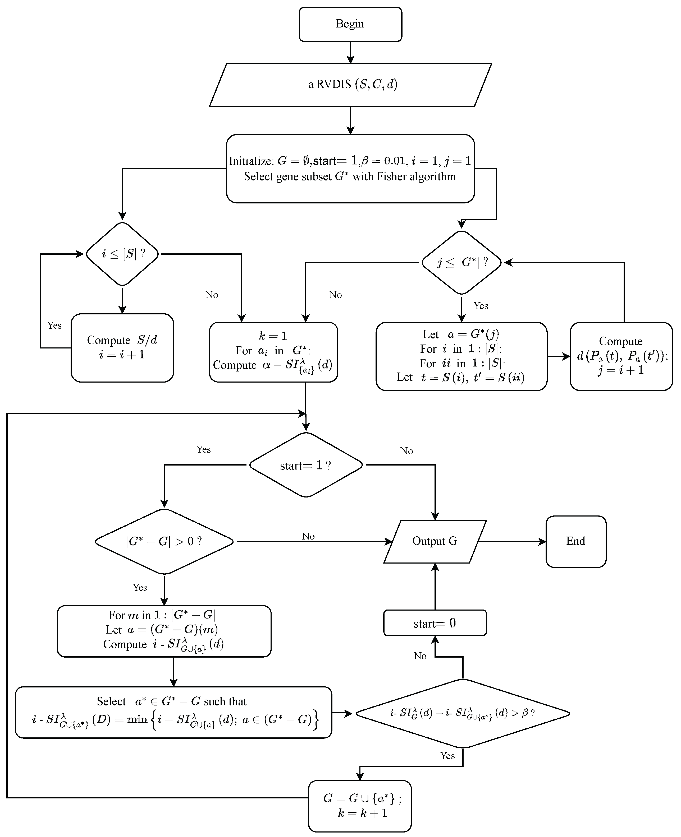
Algorithm 3: A gene selection algorithm based on relative $\theta$-self-information (Fr-$SI$) in an $scgd$-space

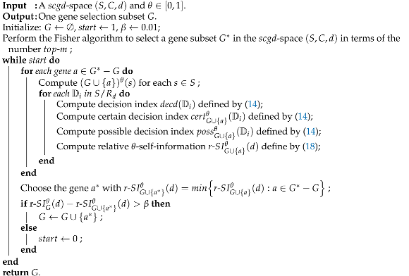
Algorithm 4: A gene selection algorithm based on the integrated-$\theta$-self-information (Fi-$SI$) in an $scgd$-space

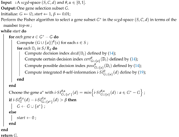
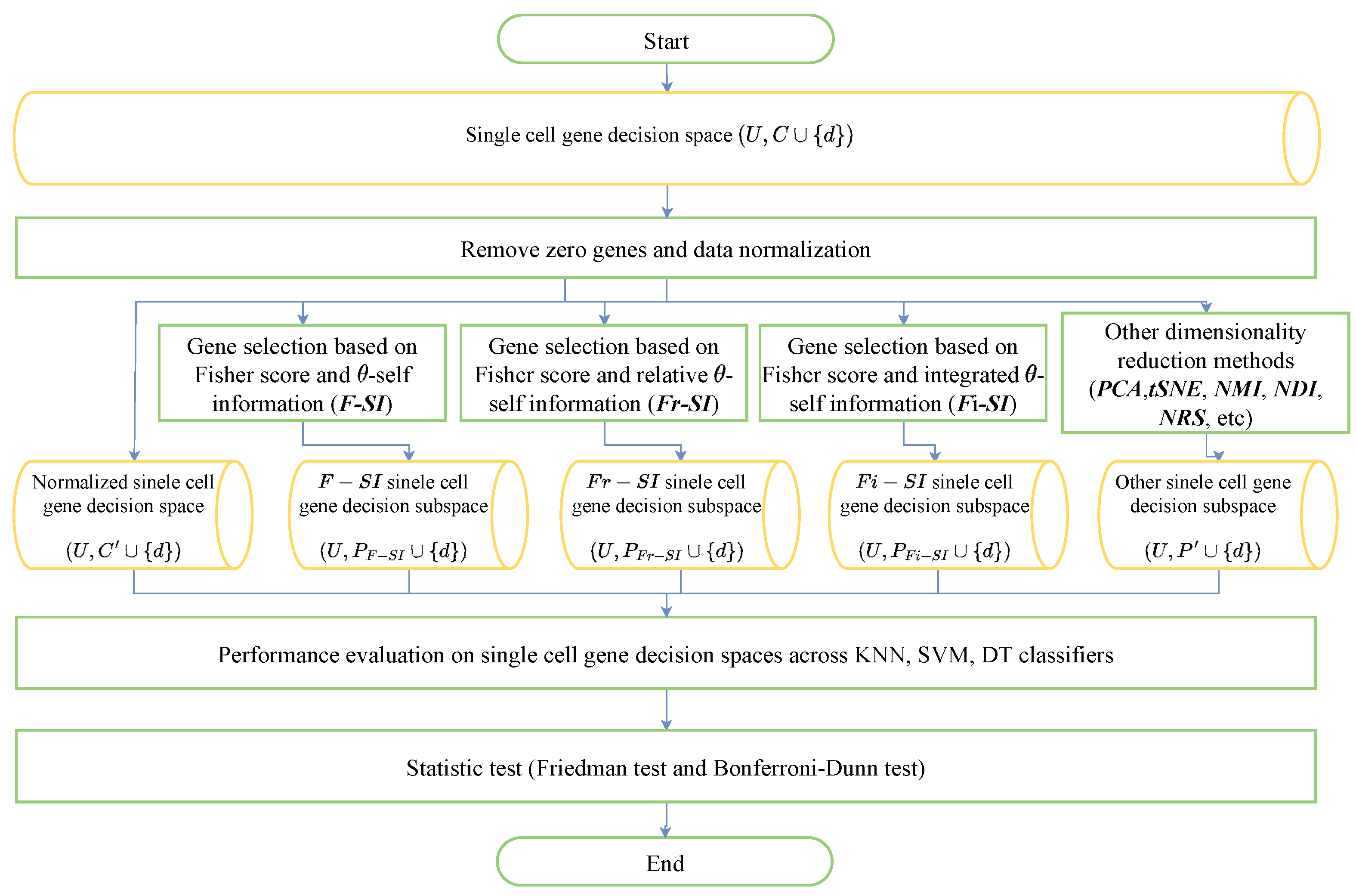
5. Experimental Analysis

This section presents experiments to evaluate performance of the proposed algorithms. The experimental flow is illustrated in Figure 3. We first employ Fisher’s score to select the preliminary genes and then implement the proposed algorithms to select subset genes on several publicly available datasets of single-cell sequencing. To evaluate the performance of proposed algorithms, the classification accuracy (ACC) of three classifiers KNN (k-nearest neighbors), SVM (support vector machine) and DT (decision tree) are taken as performance metrics. Then, two common dimension reduction methods, PCA and tSNE, are performed, and the ACC of the three classifiers are compared with those of three proposed algorithms. Moreover, we compare the proposed algorithms with three rough set-based algorithms. Finally, to eliminate randomness, two statistical tests are utilized to further verify the results.

5.1. Dataset and Preprocess

Several single-cell RNA sequencing (scRNA-seq) datasets are used to evaluate the performance of gene selection algorithms mentioned above. Detailed information on these datasets is shown in

Table 6. Datasets from scRNA sequencing.

GSE ID	Contributor	# Cells	# Raw Genes	# Class	# Preliminary Genes	Reference
GSE51372	Chen	187	19,681	7	300	Chen et al. (2014) [39]
GSE57249	Biase	56	25,680	4	100	Biase et al. (2014) [40]
GSE72612	Watanabe	95	17,151	3	1500	Watanabe et al. (2018)
GSE70657	Grover	135	15,173	2	50	Grover et al. (2016) [41]
GSE96106	Hawkins	145	33,950	2	50	Hawkins et al. (2017) [42]
GSE98852	Chiang	259	13,938	2	50	Chiang et al. (2017) [43]
GSE99701	Chen	235	24,290	5	50	Chen et al. (2017) [44]
GSE108020	Hook	473	20,930	2	50	Hook et al. (2018) [45]
GSE109556	Donega	230	22,527	2	50	Donega et al. (2018) [46]
GSE109979	Lu	329	19,685	4	850	Lu et al. (2018) [47]

. These datasets can be downloaded from the NCBI Gene Expression Omnibus (GEO) repository (https://www.ncbi.nlm.nih.gov/geo/, accessed on 20 September 2022).

Firstly, single-cell sequencing data consist of one file per sample, and it is necessary to combine these data into a matrix format. During the combination process, only genes that are present in all samples are selected to form the matrix data. Then, due to the limitations of single-cell RNA sequencing technology, there are many genes that are not expressed in single-cell gene sequencing data. The sensitivity and specificity of single-cell RNA sequencing technology are relatively low, and there is a lot of noise in RNA-seq data. These factors can lead to many genes not being expressed in single-cell gene sequencing data, and their expressed value is set to zero. Therefore, genes that have zero values in the all the samples are removed.

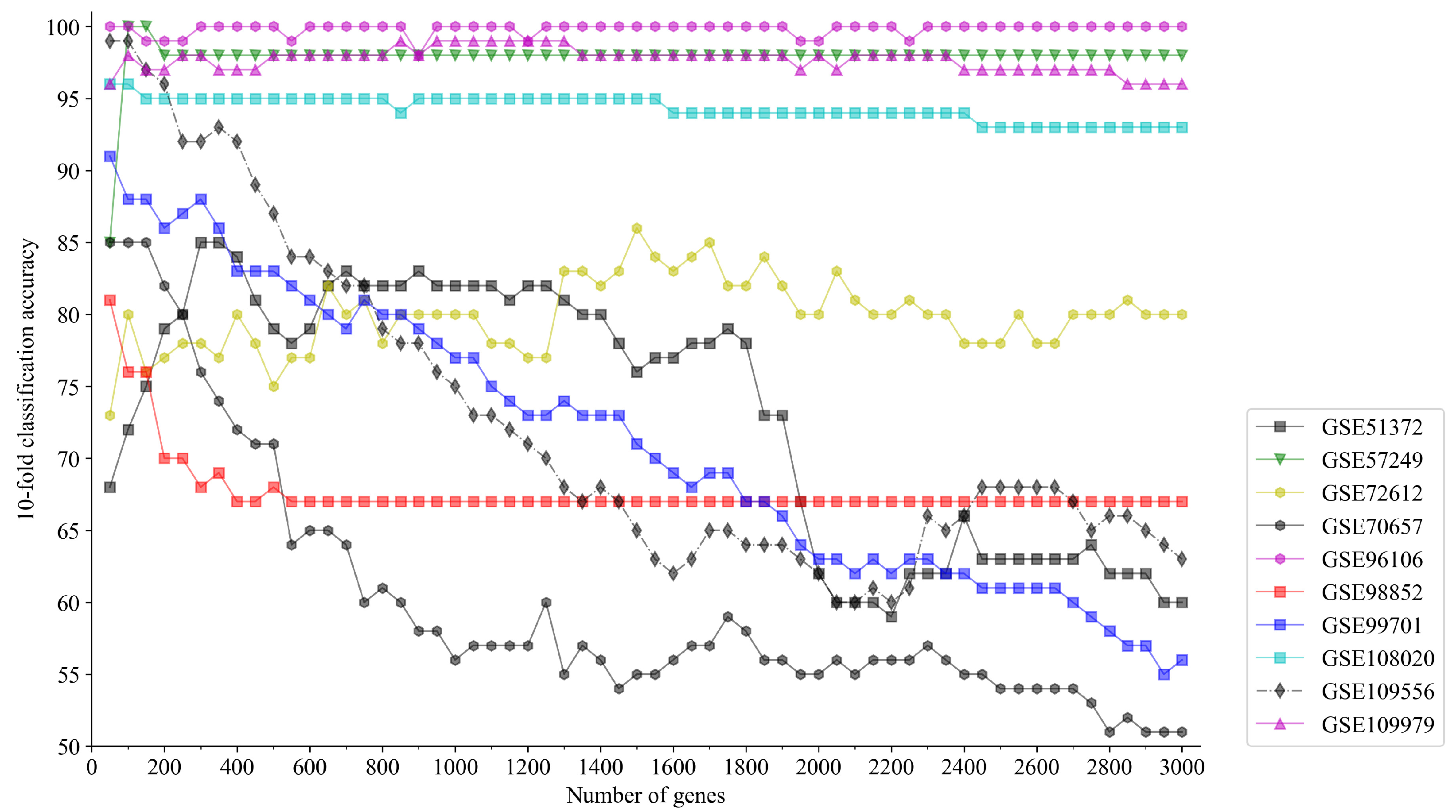
5.2. Preliminary Number of Genes

Due to the large number of genes of single-cell datasets, as a preliminary step in this study, a subset selection method based on Fisher’s score is employed to acquire a gene subset. This preliminary method calculates the Fisher’s score of each gene and selects the top k genes with highest scores among them, and the value of k is varied from 50 to 3000 in 50 increments. Afterwards, the selected genes are used as feature in a KNN (k-nearest neighbors) classifier with the model parameter $k=5$. To avoid sample randomness, ten-fold cross-validation is employed, and the accuracy is determined by the average value of its classification accuracies.

Figure 4 depicts the ten-fold classification accuracy results for the above datasets. The accuracy varies with number of genes selected by Algorithm 1. We found that the classification accuracy stabilizes as k increases. Considering that gene selection algorithms aim to maximize classification accuracy while minimizing the number of selected genes, the minimal k to reach the maximal ten-fold classification accuracy is taken as the appropriate number of preliminary genes, and a summary of the results is shown in the

Table 7. Comparisons of number of selected genes.

Datasets	Raw Data	Fisher Data	F-SI	Fr-SI	Fi-SI
GSE51372	19,681	300	14	13	16
GSE57249	25,680	100	2	2	2
GSE72612	17,151	1500	18	19	9
GSE70657	15,173	50	2	2	2
GSE96106	33,950	50	8	8	6
GSE98852	13,938	50	13	13	14
GSE99701	24,290	50	9	9	22
GSE108020	20,930	50	3	5	3
GSE109556	22,527	50	13	16	29
GSE109979	19,685	850	9	9	9

.

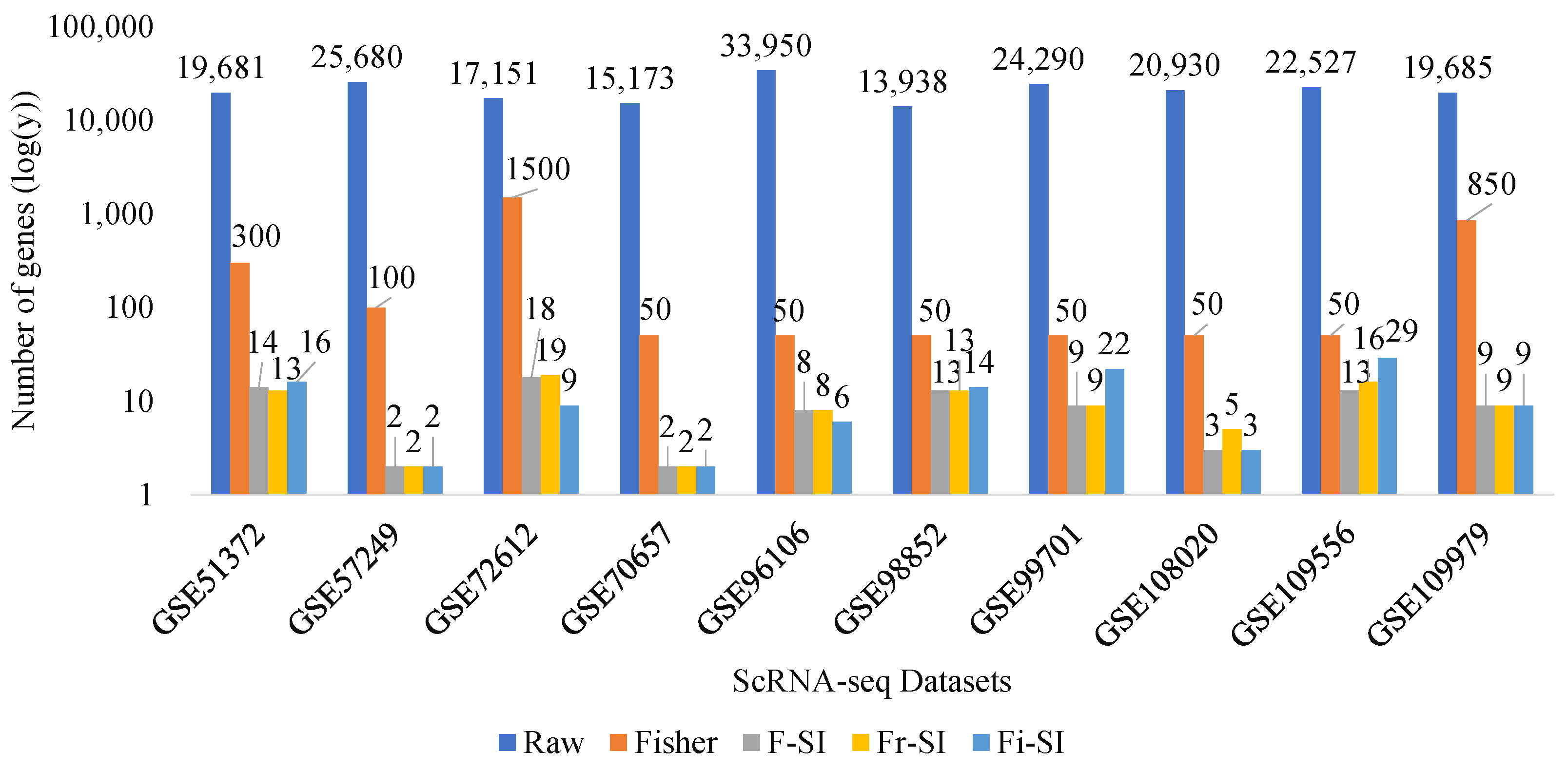
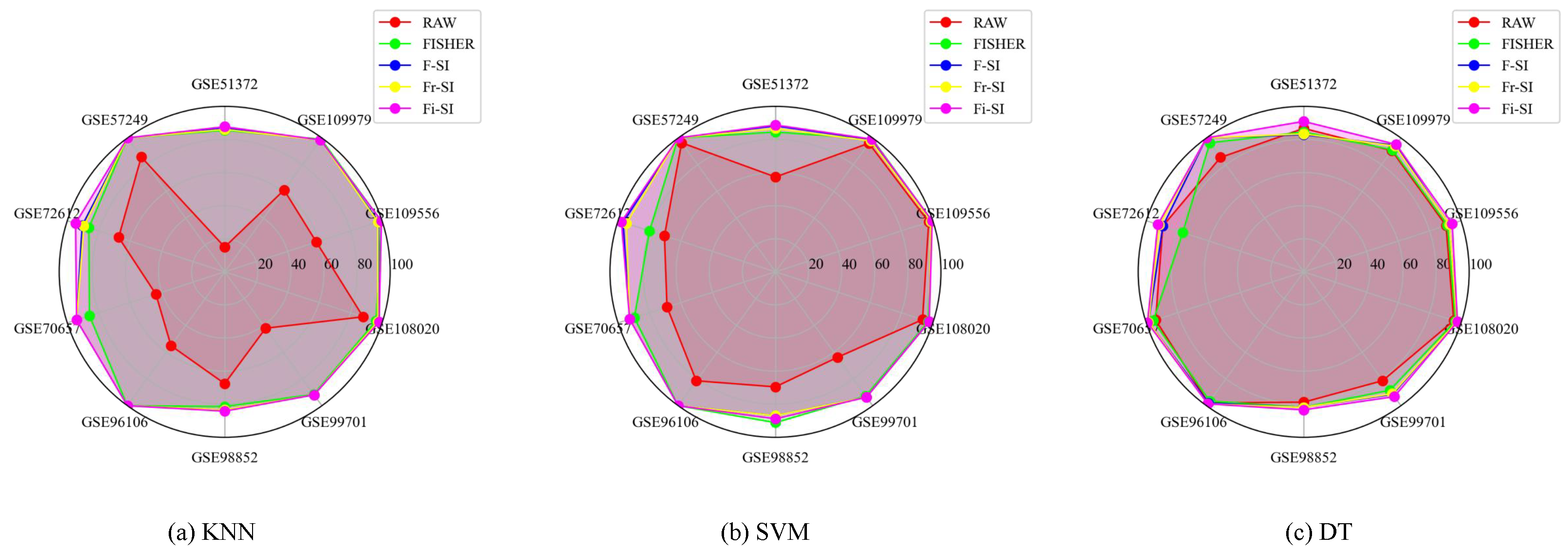
5.3. Benchmarking Compared with Raw Data and Fisher Data

In this section, the performance of proposed algorithms is compared with that of raw data and Fisher data. First, the Figure 5 and Table 7 describe the number of selected genes. The results of accuracy metrics taken by three classifiers (KNN, SVM, and DT) are shown in Figure 6 and

Table 8. Comparisons of classification accuracy (%) on KNN classifier.

Datasets	Raw	Fisher	PCA	tSNE	mRMR	ReliefF	NRS	NDI	NMI	F-SI	Fr-SI	Fi-SI
GSE51372	14.98	85.53	75.97	55.6	86.91	86.35	76.5	78.09	73.34	86.61	86.07	$\underline{87.70}$
GSE57249	85.76	$\underline{100.00}$	98.18	87.58	97.61	96.81	80.3	94.55	80.3	$\underline{100.00}$	$\underline{100.00}$	$\underline{100.00}$
GSE72612	67.37	86.32	76.84	71.58	91.65	89.71	66.32	83.16	77.89	90.53	89.47	$\underline{94.74}$
GSE70657	43.7	85.93	70.37	56.3	90.74	88.63	71.85	85.19	82.22	$\underline{94.07}$	$\underline{94.07}$	$\underline{94.07}$
GSE96106	55.17	$\underline{100.00}$	91.72	67.59	98.37	94.74	95.17	$\underline{100.00}$	97.24	$\underline{100.00}$	$\underline{100.00}$	$\underline{100.00}$
GSE98852	67.57	81.47	78.8	76.06	83.68	82.52	73.76	75.68	80.34	83.4	83.4	$\underline{84.19}$
GSE99701	42.13	91.49	77.02	63.83	90.85	90.31	73.19	90.64	80	$\underline{91.91}$	$\underline{91.91}$	$\underline{91.91}$
GSE108020	87.95	96.2	93.87	93.45	97.18	97.06	97.25	95.99	97.68	97.46	97.26	$\underline{98.10}$
GSE109556	58.26	$\underline{99.57}$	98.26	80.43	96.63	96.46	93.48	96.96	96.52	97.83	97.39	$\underline{99.57}$
GSE109979	61.08	$\underline{99.09}$	95.45	83.91	95.89	94.35	74.46	94.23	86.65	98.47	98.47	98.47

,

Table 9. Comparisons of classification accuracy (%) on SVM classifier.

Datasets	Raw	Fisher	PCA	tSNE	mRMR	ReliefF	NRS	NDI	NMI	F-SI	Fr-SI	Fi-SI
GSE51372	57.31	84.47	69	63.68	83.25	81.33	73.27	84.98	73.83	88.22	86.63	$\underline{88.75}$
GSE57249	96.36	$\underline{100.00}$	98.18	91.06	98.91	97.18	75	96.36	75	$\underline{100.00}$	$\underline{100.00}$	$\underline{100.00}$
GSE72612	70.53	80	71.58	65.26	96.15	95.11	62.11	84.21	80	96.84	94.74	$\underline{97.89}$
GSE70657	68.89	89.63	78.52	57.78	91.58	91.39	74.81	91.85	85.93	$\underline{92.59}$	$\underline{92.59}$	$\underline{92.59}$
GSE96106	81.38	$\underline{100.00}$	92.41	69.66	95.35	95.01	95.86	$\underline{100.00}$	97.93	$\underline{100.00}$	$\underline{100.00}$	$\underline{100.00}$
GSE98852	69.5	$\underline{91.13}$	78.03	75.69	87.16	83.25	78.8	81.47	83.42	86.89	86.89	88.83
GSE99701	63.83	92.77	78.3	61.28	91.48	90.19	77.02	91.91	82.55	$\underline{93.62}$	$\underline{93.62}$	$\underline{93.62}$
GSE108020	93.45	97.05	90.92	94.08	97.29	96.37	97.47	96.41	97.46	$\underline{97.68}$	$\underline{97.68}$	$\underline{97.68}$
GSE109556	97.39	$\underline{99.57}$	98.7	75.65	97.52	96.26	93.48	96.96	94.78	98.7	98.7	$\underline{99.57}$
GSE109979	96.06	$\underline{99.39}$	95.45	80.25	97.93	98.31	78.41	95.74	87.56	98.79	97.86	99.09

and

Table 10. Comparisons of classification accuracy (%) on DT classifier.

Datasets	Raw	Fisher	PCA	tSNE	mRMR	ReliefF	NRS	NDI	NMI	F-SI	Fr-SI	Fi-SI
GSE51372	86.67	84.52	72.77	55.66	87.67	85.46	79.7	78.66	86.66	82.9	83.37	$\underline{90.91}$
GSE57249	85.45	96.36	98.18	85.61	89.92	88.35	78.48	91.06	78.48	$\underline{100.00}$	$\underline{100.00}$	$\underline{100.00}$
GSE72612	89.47	76.84	76.84	81.05	91.08	89.63	69.47	82.11	77.89	89.47	91.58	$\underline{92.63}$
GSE70657	94.07	95.56	73.33	56.3	97.82	93.27	90.37	95.56	97.04	98.52	98.52	$\underline{99.26}$
GSE96106	97.93	96.55	93.1	61.38	97.95	96.83	94.48	$\underline{98.62}$	97.24	97.93	$\underline{98.62}$	$\underline{98.62}$
GSE98852	78.77	81.88	70.29	72.19	82.35	81.33	72.96	75.3	79.54	81.88	81.88	$\underline{83.42}$
GSE99701	81.28	88.51	71.06	57.87	91.83	90.07	73.62	$\underline{93.19}$	75.74	91.49	91.06	$\underline{93.19}$
GSE108020	95.35	96.41	93.24	94.3	96.35	97.13	97.68	$\underline{98.10}$	97.89	97.25	97.25	97.68
GSE109556	90.43	91.3	$\underline{99.13}$	76.09	93.38	93.61	91.74	95.22	91.3	92.61	92.61	94.35
GSE109979	90.55	91.17	92.72	91.49	93.49	92.57	71.42	88.75	82.39	94.54	93.92	$\underline{95.14}$

.

Figure 5 illustrates the number of selected genes across various datasets using different methods: raw data, Fisher, F-SI, Fr-SI, and Fi-SI. In each dataset, the number of genes selected by each method is compared, with fewer genes indicating a better method. It can be observed that number of selected genes by the proposed algorithms is significantly lower than the number chosen by raw data and Fisher data. Table 7 presented the number of genes chosen by F-SI, Fr-SI, and Fi-SI. The proposed algorithms generally outperform the raw and Fisher methods by selecting fewer genes, with F-SI and Fr-SI methods frequently showing the best performance across multiple datasets.

Meanwhile, reducing a large number of features did not result in a decrease in classification accuracy. We compared classification performance of the proposed algorithms with that of raw data and Fisher data across all datasets. Detailed results can be seen in Table 8, Table 9 and Table 10 and Figure 6. The underlined ACC values in Table 8, Table 9 and Table 10 indicate the largest ACC values with respect to raw data and Fisher data. The radar charts provided illustrate the classification accuracy of three classifiers applied to various datasets. Each spoke of the radar represents a dataset, and the distance from the center indicates the accuracy percentage, with further from the center indicating higher accuracy. We found that the performance of F-SI, Fr-SI, and Fi-SI are slightly higher than those of Fisher data and far better than those of raw data.

The significance of above results is crucial as it directly impacts the quality and interpretability of the results obtained. Proper gene selection helps in identifying key genes that are relevant to the biological question being studied, reducing noise and improving the accuracy of downstream analyses. By selecting the right genes, researchers can focus on specific biological processes, cell types, or pathways of interest, leading to more meaningful insights and discoveries from single-cell sequencing data.

5.4. Performance Comparisons with PCA and tSNE

To evaluate the performance of proposed algorithms, their results are compared with those of PCA and tSNE, two commonly used dimensionality reduction methods.

The overall classification accuracy results under three classifiers (KNN, SVM, and DT) are respectively presented in Figure 7. In comparison, the proposed Algorithms 2–4 can maintain stability of accuracy performance in different datasets. By contrast, the accuracy results for tSNE under the KNN and DT classifiers in dataset GSE51372 are only 55.60% and 55.66%, respectively, suggesting a nonstable performance among datasets.

Detailed results are presented in Table 8, Table 9 and Table 10. The underlined ACC value is the largest ACC of the algorithms. It can be found that the classification accuracy of the proposed algorithms is higher than those of PCA and tSNE through the comparison. Under three classifiers (KNN, SVM, DT), the proposed algorithms attain the largest ACC in 10, 10, and 9 of 10 datasets. It can be concluded that, under the three classifiers (KNN, SVM, and DT), the performance of the proposed algorithms is superior to that of tSNE and PCA in terms of ACC values.

5.5. Comparisons with Other Algorithms

To assess the performance of algorithms, we use three rough set-based feature selection algorithms—a neighborhood mutual information-based algorithm [24] (NMI), a neighborhood discrimination index-based algorithm [8] (NDI), and a neighborhood rough set-based algorithm [32] (NRS)—to contrast the ACC of three classifiers. Table 8, Table 9 and Table 10 present detailed results and the ACC value with underline style also means the largest ACC of algorithms. Under three classifiers (KNN, SVM, DT), the proposed algorithms attain the largest ACC in 10, 10, and 8 of 10 datasets. Specifically, Fi-SI algorithm attains the largest ACC in 10, 10, and 8 of 10 datasets. F-SI attain the largest ACC in 5, 5, and 1 datasets and Fr-SI attain the largest ACC in 5, 5, and 2 datasets. It can be found that the three proposed algorithms outperform the three contrasting algorithms in most of datasets. The ranks of ACC value displayed in

Table 11. Comparisons of rank of classification accuracy with NRS, NMI, and NDI.

Datasets	KNN						SVM						DT
	F-SI	Fr-SI	Fi-SI	NRS	NDI	NMI	F-SI	Fr-SI	Fi-SI	NRS	NDI	NMI	F-SI	Fr-SI	Fi-SI	NRS	NDI	NMI
GSE51372	2.0	3.0	1.0	5.0	4.0	6.0	2.0	3.0	1.0	6.0	4.0	5.0	4.0	3.0	1.0	5.0	6.0	2.0
GSE57249	2.0	2.0	2.0	5.5	4.0	5.5	2.0	2.0	2.0	5.5	4.0	5.5	2.0	2.0	2.0	5.5	4.0	5.5
GSE72612	2.0	3.0	1.0	6.0	4.0	5.0	2.0	3.0	1.0	6.0	4.0	5.0	3.0	2.0	1.0	6.0	4.0	5.0
GSE70657	2.0	2.0	2.0	6.0	4.0	5.0	2.0	2.0	2.0	6.0	4.0	5.0	2.5	2.5	1.0	6.0	5.0	4.0
GSE96106	2.5	2.5	2.5	6.0	2.5	5.0	2.5	2.5	2.5	6.0	2.5	5.0	4.0	2.0	2.0	6.0	2.0	5.0
GSE98852	2.5	2.5	1.0	6.0	5.0	4.0	2.5	2.5	1.0	6.0	5.0	4.0	2.5	2.5	1.0	6.0	5.0	4.0
GSE99701	2.0	2.0	2.0	6.0	4.0	5.0	2.0	2.0	2.0	6.0	4.0	5.0	3.0	4.0	1.5	6.0	1.5	5.0
GSE108020	3.0	4.0	1.0	5.0	6.0	2.0	2.0	2.0	2.0	4.0	6.0	5.0	5.5	5.5	3.5	3.5	1.0	2.0
GSE109556	2.0	3.0	1.0	6.0	4.0	5.0	2.5	2.5	1.0	6.0	4.0	5.0	4.0	3.0	2.0	5.0	1.0	6.0
GSE109979	2.0	2.0	2.0	6.0	4.0	5.0	2.0	3.0	1.0	6.0	4.0	5.0	2.0	3.0	1.0	6.0	4.0	5.0
FMR	2.2	2.6	1.55	5.75	4.15	4.75	2.15	2.45	1.55	5.75	4.15	4.95	3.25	2.95	1.6	5.5	3.35	4.35
Rank	2.0	3.0	1.0	6.0	4.0	5.0	2.0	3.0	1.0	6.0	4.0	5.0	3.0	2.0	1.0	6.0	4.0	5.0

. The penultimate and final rows depict the Friedman mean rank (FMR) and comprehensive ranks of an algorithm, where FMR is the average ranking of an algorithm. These statistics results lead to same conclusion.

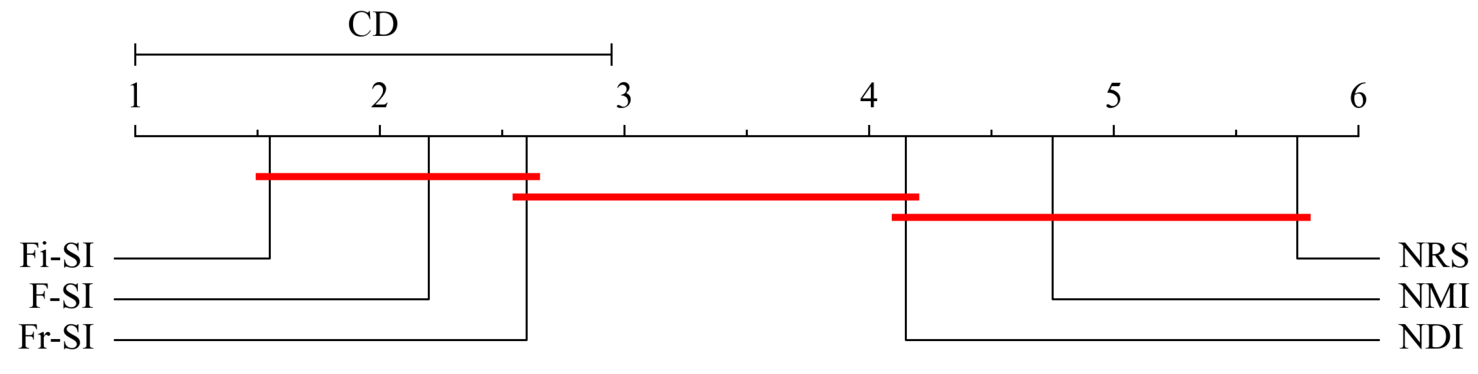
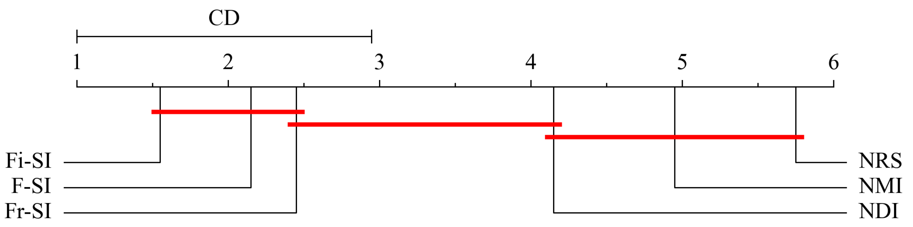
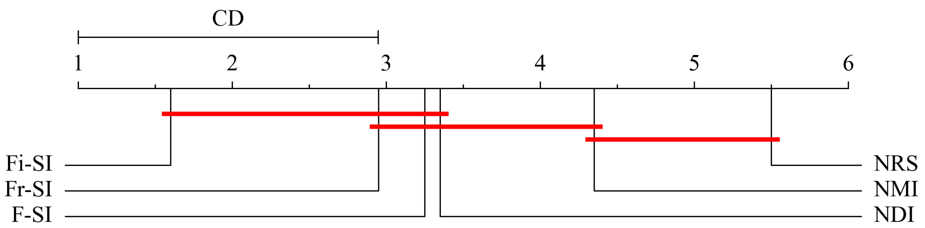
5.6. Statistical Analysis

In order to check if there were significant differences between proposed algorithms and other algorithms, the Friedman test and the Bonferroni–Dunn test are utilized to analyze the ACC results with NDI, NMI, and NRS.

The Friedman test is used to determine whether all algorithms have the same performance. The Friedman statistic is formulated as follows.

$${\chi }_F^2={\displaystyle \frac{12N}{k(K+1)}}\left(\sum _{i=1}^k{r}_i^2-{\displaystyle \frac{k{(k+1)}^2}{4}}\right),$$

(22)

where k denotes the number of algorithms, N denotes the number of datasets, $r_i$ denotes the mean rank of the i-th algorithm. As the Friedman test is too conservative, it is replaced by the $F_F$ statistic.

$$F_F={\displaystyle \frac{(N-1){\chi }_F^2}{N(k-1)-{\chi }_F^2}}.$$

(23)

The $F_F$ follows a Fisher distribution with $k-1$ and $(k-1)(N-1)$ degrees of freedom.

The calculation of the Friedman statistic value is facilitated by the aforementioned ranks in Table 11. The FMR in Table 11 allows for the computation of the corresponding statistics ${\chi }_F$ and ${\mathcal{F}}_F$ under KNN, SVM, and DT classifiers using Formulas (22) and (23).

Table 12. Comparison of value of ${\chi }_F^2$ and $F_F$ for classification accuracy under 3 classifiers with NDI, NMI, and NRS.

Values	KNN	SVM	DT
${\chi }_F^2$	41.45	44.59	25.95
$F_F$	43.69	74.25	9.71

displays two sets of statistics that correspond to Table 11.

The null hypothesis of Friedman statistic is that the classification performance of the five algorithms are identical. If statistic $F_F>F_{\alpha }(k-1,(k-1)(N-1))$, then the algorithms have different performance. Table 11 present the quantities of algorithms and datasets, which are 6 and 10, respectively. These values correspond to $k=6$ and $N=10$ in Formulas (22) and (23). The critical value of $F_{0.1}(5,45)=1.980$ at the significance level $\alpha =0.1$. From Table 12, it can be found that three statistics are all larger than that. Accordingly, the performances of six algorithms vary statistically significantly among KNN, DT, and SVM classifiers.

To judge whether the performance of the proposed algorithms exceed those of NDI, NMI and NRS, the Bonferroni–Dunn test is employed as post hoc analysis. In order to determine which algorithm differs significantly from the control algorithm, pairwise comparisons are performed between the algorithms. Following is the formula for the critical distance statistic (CD):

$$C{D}_{\alpha }=q_{\alpha }^k\sqrt{{\displaystyle \frac{k(k+1)}{6N}}},$$

(24)

where $q_{\alpha }$ satisfies Tukey distributions with k degrees of freedom. Statistically, if the absolute FMR difference between algorithms is greater than $C{D}_{\alpha }$, there is then a better algorithm than the other.

In terms of the Formula (24), the critical value $C{D}_{0.1}=1.94$ if $\alpha =0.1$, $k=6$ and $N=10$. Figure 8, Figure 9 and Figure 10 show the critical diagram of ranking all four algorithms. The axis represents the average ranking of each algorithm across all tested datasets. Lower ranks are generally better, indicating higher performance. The red horizontal line indicates the threshold of statistical significance. If the ranges of two algorithms do not overlap by more than this CD, their performance difference is considered statistically significant. It can be concluded from these figures that for KNN and SVM classifiers, Fi-$SI$ outperforms NMI NRS and NDI but does not perform better than NDI. For DT classifier, Fi-$SI$ does not perform better than NDI, but it outperforms NMI and NRS.

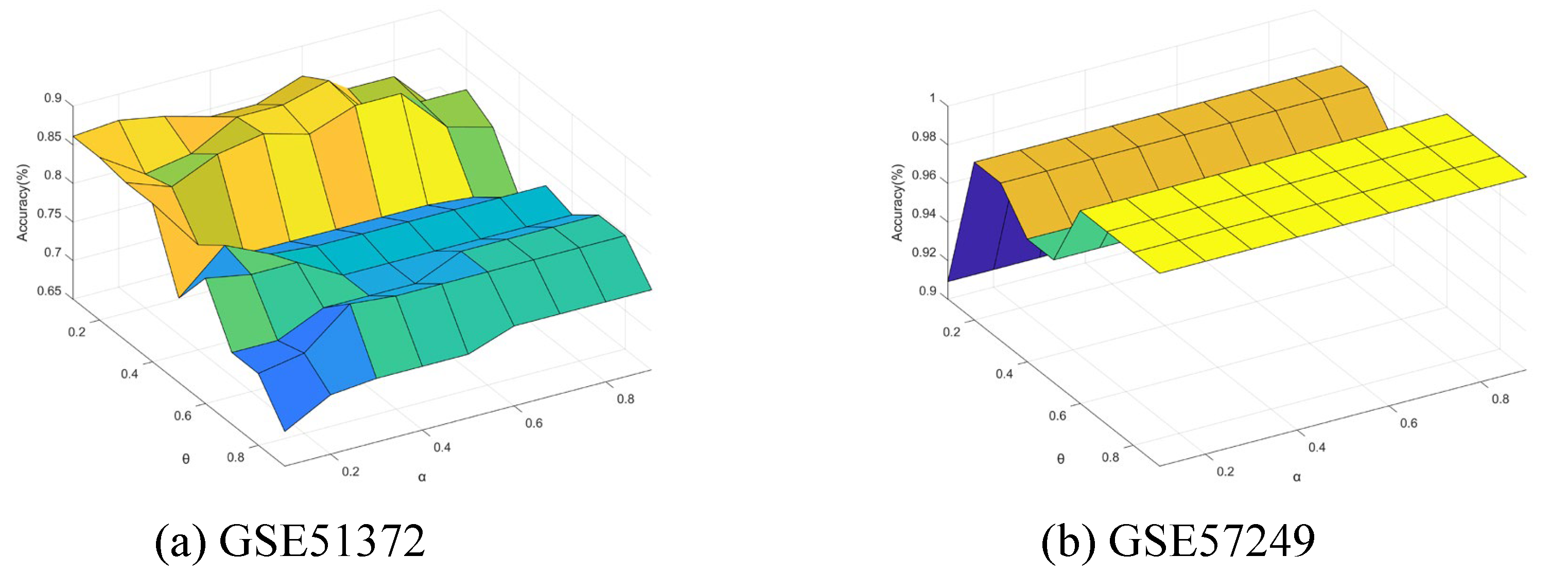
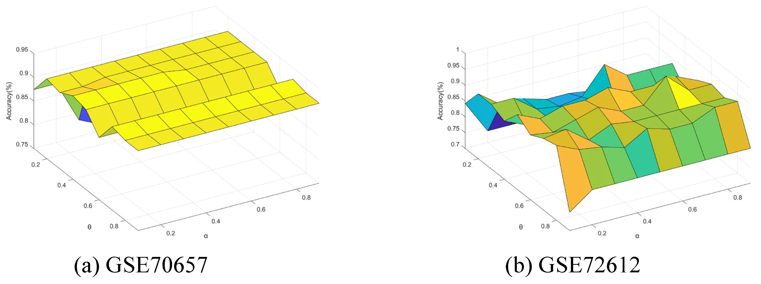
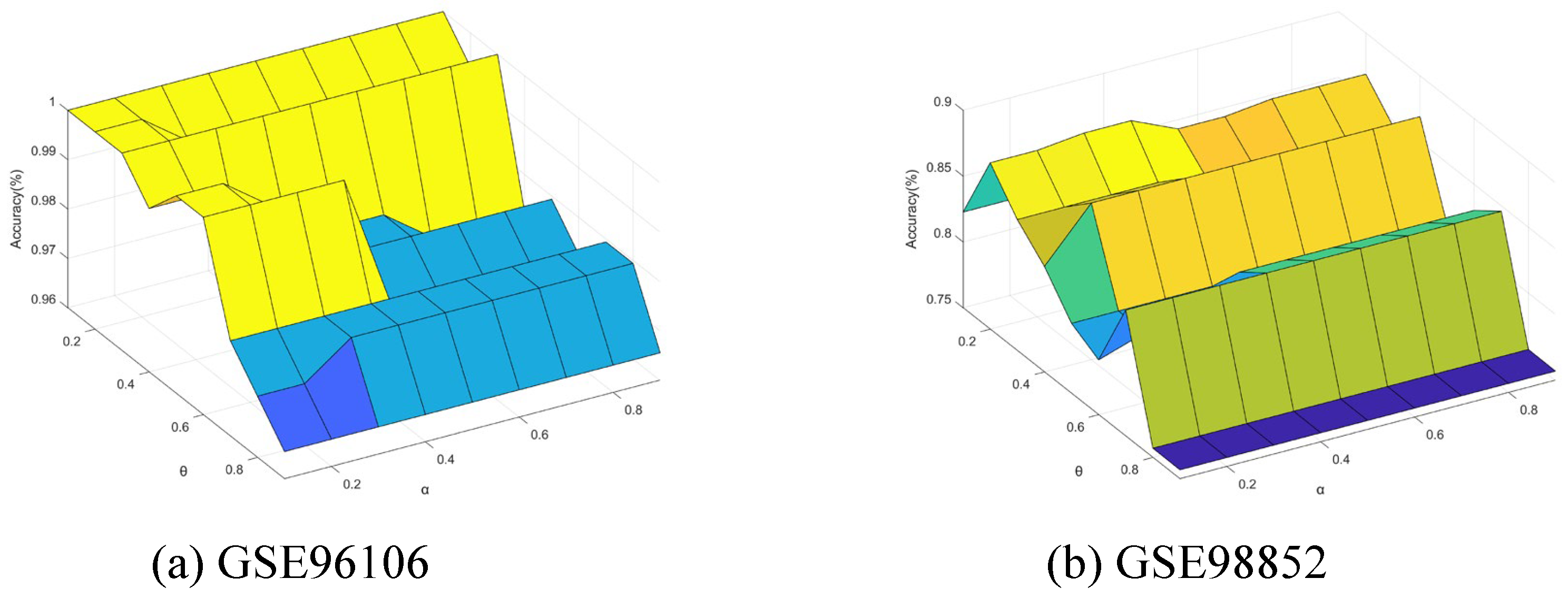
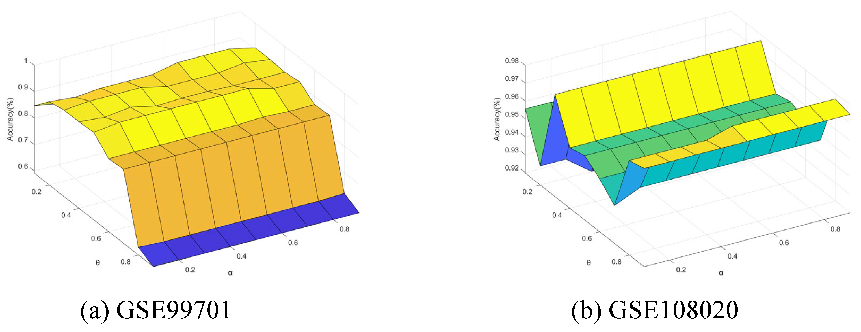
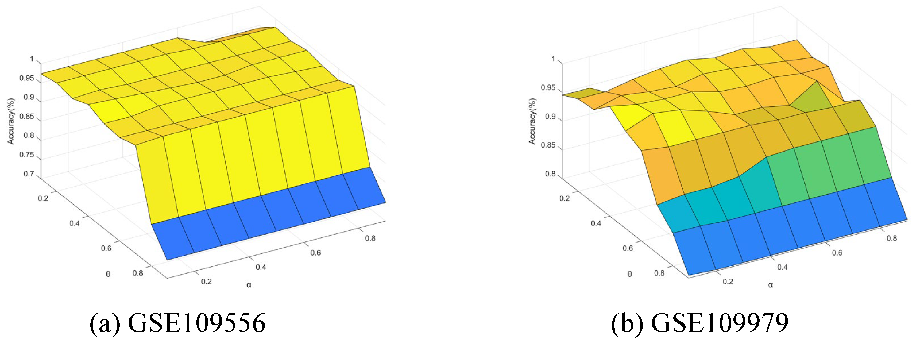
5.7. Sensitivity Analysis

Finally, we conducted further experiments to present the performance change with the neighborhood parameter $\theta$ and integration parameter $\alpha$ of Algorithm 4. The parameters $\theta$ and $\alpha$ were varied from 0.1 to 0.9 with step of 0.1. Figure 11, Figure 12, Figure 13, Figure 14 and Figure 15 show the ACC curves for different datasets with SVM classifier. The results of KNN and DT are similar to SVM.

The results indicate that higher accuracy is achievable over an expanded area in the majority of cases. Concurrently, most datasets exhibit stability within their respective regions. Consequently, these figures facilitate the selection of appropriate values for each dataset.

It is observed that numerous datasets achieve optimal accuracy as $\alpha$ varies. By taking into account both the upper and lower approximations of the decision, the characterization of the knowledge can be enhanced, thereby leading to improved classification accuracy.

Specifically, in the results from GSE57249, the minimal variation in accuracy with respect to the parameter $\alpha$ indicates that the $S{I}_G^{\theta }\left(d\right)$ and $p-S{I}_G^{\theta }\left(d\right)$, which measure classification certainty (through the lower approximation) and likelihood (through the upper approximation), respectively, are highly correlated. This correlation arises when samples from different classes are fully separable within the attribute space, resulting in clear-cut partitions of neighborhoods or equivalence classes.

6. Conclusions

Gene selection is a valuable method for discovering gene subsets that are meaningful to understand disease. This paper proposed three self-information-based gene selection algorithms to sufficiently considering information contained in the upper and lower approximations that facilitate the selection of optimal gene subsets. The main highlights of this paper are as follows: (1) By defining the tolerance relation on the cell set, the tolerance class and rough approximations are constructed, overcoming the shortcomings of the traditional rough set model. (2) Considering both lower and upper approximations, three uncertainty measures (self-information, relative self-information and integrated self-information) are defined that further take advantage of upper approximation and may result in accurate gene selection. (3) Several open single-cell datasets downloaded from GEO were preprocessed and experiments on them show that classification performance of the proposed algorithms can be improved by selecting appropriate genes related to classification.

The findings of experiment results reveal that the $Fi-SI$ method attains an impressive average classification accuracy of 93.7% when utilizing the KNN algorithm while simultaneously selecting a significantly reduced number of genes compared to the gene selection achieved by Fisher’s score. There is still room for further optimization and improvement of the designed algorithms: (1) When processing datasets containing large numbers of cells and genes, increasing efficiency and reducing time of execution is needed; (2) Preliminary gene selection based on Fisher’s score may discard meaningful genes that achieve a low Fisher score. Investigation will need to be performed on whether preliminary selection can be removed to achieve a more comprehensive result if efficiency and time are allowed. In the future, we will investigate the application of the proposed algorithms to other types of data, such as biomedical data and image data. We will integrate ensemble methods like random forest to compare feature importance rankings with self-information metrics, further bridging uncertainty-aware selection and ensemble learning. We will use deep learning and mutual information bottleneck methods to gene selection.

References

1. Ayub, S.; Shabir, M.; Riaz, M.; Karaaslan, F.; Marinkovic, D.; Vranjes, D. Linear Diophantine Fuzzy Rough Sets on Paired Universes with Multi Stage Decision Analysis. Axioms 2022, 11, 686. [Google Scholar] [CrossRef]
2. Ayub, S.; Shabir, M.; Riaz, M.; Mahmood, W.; Bozanic, D.; Marinkovic, D. Linear Diophantine Fuzzy Rough Sets: A New Rough Set Approach with Decision Making. Symmetry 2022, 14, 525. [Google Scholar] [CrossRef]
3. Pawlak, Z. Rough sets. Int. J. Comput. Inf. Sci. 1982, 11, 341–356. [Google Scholar] [CrossRef]
4. Shannon, C.E. A mathematical theory of communication. Bell Syst. Tech. J. 1948, 27, 379–423. [Google Scholar] [CrossRef]
5. Wang, C.; Huang, Y.; Shao, M.; Hu, Q.; Chen, D. Feature selection based on neighborhood self-information. IEEE Trans. Cybern. 2019, 50, 4031–4042. [Google Scholar] [CrossRef] [PubMed]
6. Zhang, Q.; Chen, Y.; Zhang, G.; Li, Z.; Chen, L.; Wen, C.F. New uncertainty measurement for categorical data based on fuzzy information structures: An application in attribute reduction. Inf. Sci. 2021, 580, 541–577. [Google Scholar] [CrossRef]
7. Li, Z.; Zhang, P.; Ge, X.; Xie, N.; Zhang, G.; Wen, C.F. Uncertainty measurement for a fuzzy relation information system. IEEE Trans. Fuzzy Syst. 2019, 27, 2338–2352. [Google Scholar] [CrossRef]
8. Navarrete, J.; Viejo, D.; Cazorla, M. Color smoothing for RGB-D data using entropy information. Appl. Soft Comput. 2016, 46, 361–380. [Google Scholar] [CrossRef]
9. Hempelmann, C.F.; Sakoglu, U.; Gurupur, V.P.; Jampana, S. An entropy-based evaluation method for knowledge bases of medical information systems. Expert Syst. Appl. 2016, 46, 262–273. [Google Scholar] [CrossRef]
10. Delgado, A.; Romero, I. Environmental conflict analysis using an integrated grey clustering and entropy-weight method: A case study of a mining project in Peru. Environ. Model. Softw. 2016, 77, 108–121. [Google Scholar] [CrossRef]
11. Zeng, A.; Li, T.; Liu, D.; Zhang, J.; Chen, H. A fuzzy rough set approach for incremental feature selection on hybrid information systems. Fuzzy Sets Syst. 2015, 258, 39–60. [Google Scholar] [CrossRef]
12. Kim, K.J.; Jun, C.H. Rough set model based feature selection for mixed-type data with feature space decomposition. Expert Syst. Appl. 2018, 103, 196–205. [Google Scholar] [CrossRef]
13. Wang, C.; Wang, Y.; Shao, M.; Qian, Y.; Chen, D. Fuzzy rough attribute reduction for categorical data. IEEE Trans. Fuzzy Syst. 2019, 28, 818–830. [Google Scholar] [CrossRef]
14. Dai, J.H.; Hu, H.; Zheng, G.J.; Hu, Q.H.; Han, H.F.; Shi, H. Attribute reduction in interval-valued information systems based on information entropies. Front. Inf. Technol. Electron. Eng. 2016, 17, 919–928. [Google Scholar] [CrossRef]
15. Singh, S.; Shreevastava, S.; Som, T.; Somani, G. A fuzzy similarity-based rough set approach for attribute selection in set-valued information systems. Soft Comput. 2020, 24, 4675–4691. [Google Scholar] [CrossRef]
16. Sang, B.; Chen, H.; Yang, L.; Li, T.; Xu, W. Incremental feature selection using a conditional entropy based on fuzzy dominance neighborhood rough sets. IEEE Trans. Fuzzy Syst. 2021, 30, 1683–1697. [Google Scholar] [CrossRef]
17. Huang, Z.; Li, J. Discernibility Measures for Fuzzy β Covering and Their Application. IEEE Trans. Cybern. 2022, 52, 9722–9735. [Google Scholar] [CrossRef]
18. Jia, X.; Rao, Y.; Shang, L.; Li, T. Similarity-based attribute reduction in rough set theory: A clustering perspective. Int. J. Mach. Learn. Cybern. 2020, 11, 1047–1060. [Google Scholar] [CrossRef]
19. Li, Z.; Qu, L.; Zhang, G.; Xie, N. Attribute selection for heterogeneous data based on information entropy. Int. J. Gen. Syst. 2021, 50, 548–566. [Google Scholar] [CrossRef]
20. Wang, Y.; Chen, X.; Dong, K. Attribute reduction via local conditional entropy. Int. J. Mach. Learn. Cybern. 2019, 10, 3619–3634. [Google Scholar] [CrossRef]
21. Yuan, Z.; Chen, H.; Zhang, P.; Wan, J.; Li, T. A novel unsupervised approach to heterogeneous feature selection based on fuzzy mutual information. IEEE Trans. Fuzzy Syst. 2021, 30, 3395–3409. [Google Scholar] [CrossRef]
22. Chen, Z.; Liu, K.; Yang, X.; Fujita, H. Random sampling accelerator for attribute reduction. Int. J. Approx. Reason. 2022, 140, 75–91. [Google Scholar] [CrossRef]
23. Jiang, Z.; Liu, K.; Yang, X.; Yu, H.; Fujita, H.; Qian, Y. Accelerator for supervised neighborhood based attribute reduction. Int. J. Approx. Reason. 2020, 119, 122–150. [Google Scholar] [CrossRef]
24. Chen, Y.; Liu, K.; Song, J.; Fujita, H.; Yang, X.; Qian, Y. Attribute group for attribute reduction. Inf. Sci. 2020, 535, 64–80. [Google Scholar] [CrossRef]
25. Buettner, F.; Natarajan, K.N.; Casale, F.P.; Proserpio, V.; Scialdone, A.; Theis, F.J.; Teichmann, S.A.; Marioni, J.C.; Stegle, O. Computational analysis of cell-to-cell heterogeneity in single-cell RNA-sequencing data reveals hidden subpopulations of cells. Nat. Biotechnol. 2015, 33, 155–160. [Google Scholar] [CrossRef]
26. Chung, W.; Eum, H.H.; Lee, H.O.; Lee, K.M.; Lee, H.B.; Kim, K.T.; Ryu, H.S.; Kim, S.; Lee, J.E.; Park, Y.H.; et al. Single-cell RNA-seq enables comprehensive tumour and immune cell profiling in primary breast cancer. Nat. Commun. 2017, 8, 15081. [Google Scholar] [CrossRef]
27. Bommert, A.; Welchowski, T.; Schmid, M.; Rahnenführer, J. Benchmark of filter methods for feature selection in high-dimensional gene expression survival data. Briefings Bioinform. 2021, 23, bbab354. [Google Scholar] [CrossRef]
28. Li, Z.; Zhang, J.; Liu, F.; Wen, C.F. Uncertainty measurement for single cell RNA-seq data via Gaussian kernel: Application to unsupervised gene selection. Eng. Appl. Artif. Intell. 2024, 130, 107707. [Google Scholar] [CrossRef]
29. Sharma, A.; Rani, R. C-HMOSHSSA: Gene selection for cancer classification using multi-objective meta-heuristic and machine learning methods. Comput. Methods Programs Biomed. 2019, 178, 219–235. [Google Scholar] [CrossRef]
30. Zhang, Q.; Zhao, Z.; Liu, F.; Li, Z. Uncertainty measurement for single cell RNA-seq data based on class-consistent technology with application to semi-supervised gene selection. Appl. Soft Comput. 2023, 146, 110645. [Google Scholar] [CrossRef]
31. Sun, L.; Zhang, X.Y.; Qian, Y.H.; Xu, J.C.; Zhang, S.G.; Tian, Y. Joint neighborhood entropy-based gene selection method with fisher score for tumor classification. Appl. Intell. 2019, 49, 1245–1259. [Google Scholar] [CrossRef]
32. Sheng, J.; Li, W.V. Selecting gene features for unsupervised analysis of single-cell gene expression data. Briefings Bioinform. 2021, 22, bbab295. [Google Scholar] [CrossRef]
33. Zhang, J.; Zhang, G.; Li, Z.; Qu, L.; Wen, C.F. Feature selection in a neighborhood decision information system with application to single cell RNA data classification. Appl. Soft Comput. 2021, 113, 107876. [Google Scholar] [CrossRef]
34. Li, Z.; Feng, J.; Zhang, J.; Liu, F.; Wang, P.; Wen, C.F. Gaussian kernel based gene selection in a single cell gene decision space. Inf. Sci. 2022, 610, 1029–1057. [Google Scholar] [CrossRef]
35. Zhang, J.; Yu, G.; Huang, D.; Wang, Y. Gene selection in a single cell gene decision space based on class-consistent technology and fuzzy rough iterative computation model. Appl. Intell. 2023, 53, 30113–30132. [Google Scholar] [CrossRef]
36. Zhang, Q.; Wang, P.; Pedrycz, W.; Li, Z. Neighborhood entropy guided by a decision attribute and its applications in multi-source information fusion and attribute selection. Appl. Soft Comput. 2024, 167, 112380. [Google Scholar] [CrossRef]
37. Ma, X.; Liu, J.; Wang, P.; Yu, W.; Hu, H. Feature selection for hybrid information systems based on fuzzy ß covering and fuzzy evidence theory. J. Intell. Fuzzy Syst. 2024, 46, 4219–4242. [Google Scholar]
38. Yu, W.; Ma, X.; Zhang, Z.; Zhang, Q. A Method for Fast Feature Selection Utilizing Cross-Similarity within the Context of Fuzzy Relations. cmc-Comput. Mater. Contin. 2025, 83, 1195–1218. [Google Scholar] [CrossRef]
39. Ting, D.T.; Wittner, B.S.; Ligorio, M.; Jordan, N.V.; Shah, A.M.; Miyamoto, D.T.; Aceto, N.; Bersani, F.; Brannigan, B.W.; Xega, K. et al. Single-cell rna sequencing identifies extracellular matrix gene expression by pancreatic circulating tumor cells. Cell Rep. 2014, 8, 1905–1918. [Google Scholar] [CrossRef]
40. Biase, F.H.; Cao, X.; Zhong, S. Cell fate inclination within 2-cell and 4-cell mouse embryos revealed by single-cell rna sequencing. Genome Res. 2014, 24, 1787–1796. [Google Scholar] [CrossRef]
41. Grover, A.; Sanjuan-Pla, A.; Thongjuea, S.; Carrelha, J.; Giustacchini, A.; Gambardella, A.; Macaulay, I.; Mancini, E.; Luis, T.C.; Mead, A. et al. Single-cell rna sequencing reveals molecular and functional platelet bias of aged haematopoietic stem cells. Nat. Commun. 2016, 7, 11075. [Google Scholar] [CrossRef] [PubMed]
42. Hawkins, F.; Kramer, P.; Jacob, A.; Driver, I.; Thomas, D.C.; McCauley, K.B.; Skvir, N.; Crane, A.M.; Kurmann, A.A.; Hollenberg, A.N.; et al. Prospective isolation of nkx2-1–expressing human lung progenitors derived from pluripotent stem cells. J. Clin. Investig. 2017, 127, 2277–2294. [Google Scholar] [CrossRef] [PubMed]
43. Chiang, D.; Chen, X.; Jones, S.M.; Wood, R.A.; Sicherer, S.H.; Burks, A.W.; Leung, D.Y.; Agashe, C.; Grishin, A.; Dawson, P.; et al. Single-cell profiling of peanut-responsive t cells in patients with peanut allergy reveals heterogeneous effector th2 subsets. J. Allergy And Clinical Immunol. 2018, 141, 2107–2120. [Google Scholar] [CrossRef] [PubMed]
44. Chen, L.; Lee, J.W.; Chou, C.-L.; Nair, A.V.; Battistone, M.A.; Păunescu, T.G.; Merkulova, M.; Breton, S.; Verlander, J.W.; Wall, S.M.; et al. Transcriptomes of major renal collecting duct cell types in mouse identified by single-cell rna-seq. Proc. Natl. Acad. Sci. USA 2017, 114, E9989–E9998. [Google Scholar] [CrossRef]
45. Hook, P.W.; McClymont, S.A.; Cannon, G.H.; Law, W.D.; Morton, A.J.; Goff, L.A.; McCallion, A.S. Single-cell rna-seq of dopaminergic neurons informs candidate gene selection for sporadic parkinson’s disease. bioRxiv 2017, 148049. [Google Scholar]
46. Donega, V.; Marcy, G.; Giudice, Q.L.; Zweifel, S.; Angonin, D.; Fiorelli, R.; Abrous, D.N.; Rival-Gervier, S.; Koehl, M.; Jabaudon, D.; et al. Transcriptional dysregulation in postnatal glutamatergic progenitors contributes to closure of the cortical neurogenic period. Cell Rep. 2018, 22, 2567–2574. [Google Scholar] [CrossRef]
47. Lu, J.; Baccei, A.; da Rocha, E.L.; Guillermier, C.; McManus, S.; Finney, L.A.; Zhang, C.; Steinhauser, M.L.; Li, H.; Lerou, P.H. Single-cell rna sequencing reveals metallothionein heterogeneity during hesc differentiation to definitive endoderm. Stem Cell Res. 2018, 28, 48–55. [Google Scholar] [CrossRef]
Figure 1. Flowchart of this paper.
Mathematics 13 01829 g001
Figure 2. The framework of Algorithm 4.
Mathematics 13 01829 g002
Figure 3. Experimental flow.
Mathematics 13 01829 g003
Figure 4. Classification accuracy of KNN based on k genes with top Fisher’s score.
Mathematics 13 01829 g004
Figure 5. Comparisons of number of selected genes.
Mathematics 13 01829 g005
Figure 6. Comparisons of classification accuracy (%) of three classifier (KNN (a), SVM (b), DT (c)) with raw data and Fisher data.
Mathematics 13 01829 g006
Figure 7. Comparison of classification accuracy (%) for three classifiers (KNN (a), SVM (b), DT (c)) with PCA and tSNE.
Mathematics 13 01829 g007
Figure 8. KNN classifier critical diagram for Bonferroni–Dunn test ranking all algorithms.
Mathematics 13 01829 g008
Figure 9. SVM classifier critical diagram for Bonferroni–Dunn test ranking all algorithms.
Mathematics 13 01829 g009
Figure 10. DT classifier critical diagram for Bonferroni–Dunn test ranking all algorithms.
Mathematics 13 01829 g010
Figure 11. Accuracy varying with θ and α (GSE51372 and GSE57249).
Mathematics 13 01829 g011
Figure 12. Accuracy varying with θ and α (GSE70657 and GSE72612).
Mathematics 13 01829 g012
Figure 13. Accuracy varying with θ and α (GSE96106 and GSE98852).
Mathematics 13 01829 g013
Figure 14. Accuracy varying with θ and α (GSE99701 and GSE108020).
Mathematics 13 01829 g014
Figure 15. Accuracy varying with θ and α (GSE109556 and GSE109979).
Mathematics 13 01829 g015