Managing Risk Across Time: An Intertemporal Spectral Risk Measures Framework for Multi-Period Portfolio Optimization

Abstract

This paper introduces a novel framework for multi-period portfolio optimization that incorporates intertemporal spectral risk measures (ISRMs). The model dynamically manages risk by considering both tail risk, through spectral risk measures, and overall portfolio volatility, through variance, across multiple time periods. This approach allows investors to specify time-varying risk preferences via a spectral function, making it particularly suitable for investors with evolving risk management needs. We develop an efficient solution methodology based on the Progressive Hedging Algorithm (PHA), enhanced with specialized reformulations to handle linkage objectives and constraints inherent in the multi-period setting. We establish the theoretical convergence properties of our algorithm, demonstrating a q-linear convergence rate under mild conditions. Numerical experiments validate the effectiveness of our approach, showing that the intertemporal weighting scheme provides more consistent risk management across the investment horizon compared to terminal-focused strategies. Notably, our approach exhibits superior downside risk protection, as evidenced by improved Sortino and Omega ratios, and generates more balanced wealth distributions with moderate tails. These findings offer valuable insights and practical tools for investors seeking to implement dynamic risk-management strategies that account for both intermediate and terminal objectives.

1. Introduction

The mean-variance (MV) portfolio selection model, introduced by [1], has been widely utilized in both academic research and investment practice. However, a drawback of the MV formulation is its symmetric nature, which penalizes both gains and losses equally. To address this issue, various risk measures have been introduced into the portfolio optimization framework. The concept of a coherent risk measure [2], along with its extension, the convex risk measure [3], has laid down fundamental principles for defining more reasonable risk measures. Along with the development of modern risk measures, the mean-risk portfolio optimization models have been extensively studied under the frameworks of static and dynamic portfolio optimizations (e.g., [4,5,6,7,8,9,10,11]). Recently, researchers (e.g., [12,13,14]) have also demonstrated the successful application of the downside risk-based models in portfolio insurance management. Among these studies, one particular direction focuses on the portfolio optimization model with multiple hybrid risk measures (e.g., [10,11,15,16,17]). This line of research is motivated by the fact that, in cases where the distribution of portfolio returns is asymmetrical and non-Gaussian, solely minimizing variance is insufficient for effectively managing downside risk.

This paper adopts a similar approach to previous studies, exploring the dynamic mean-risk portfolio decision model by integrating both the mean-variance (MV) formulation and the spectral risk measure (SRM). Building on the foundational work of [18], SRM calculates risk as a weighted average of the quantiles of the return (or wealth) distribution. When the weighting function, also referred to as the spectrum, satisfies certain mild conditions, SRM qualifies as a coherent risk measure, as demonstrated by [9,18]. While SRM represents a specific case within the broader spectrum of risk measures, such as the distortion risk measure or weighted VaR [7,9], it possesses several advantageous properties, including convexity, tractability, and flexibility when selecting the spectrum function. The power of distortion functions to capture nuanced risk preferences is further highlighted by their use in other advanced frameworks, such as distributionally robust optimization under distorted expectations [19]. These attributes make SRM a particularly suitable choice for constructing portfolio optimization models.

In this study, we propose a novel hybrid portfolio optimization model that integrates multiple risk measures, specifically the dynamic SRM-MV portfolio optimization model. The integration of SRM into the dynamic MV framework is significant for several reasons. First, it enhances the ability to shape the distribution of terminal wealth, particularly by strengthening the management of downside risk in the loss domain. Recent research by [20] highlights that the terminal wealth distribution under a dynamic MV policy may exhibit a long tail in the loss domain, underscoring the importance of incorporating downside risk measures to control tail risk. Second, the inclusion of SRM diminishes the dominance of variance in the objective function, thereby alleviating the conservatism associated with variance-based risk management within the gains domain. This hybrid approach not only improves the robustness of portfolio optimization but also aligns more closely with real-world risk management needs.

On the other hand, in the traditional multi-period portfolio selection model, the focus is primarily on the risk and return associated with terminal wealth. However, in real-world investment scenarios, investors are also concerned with the performance of the portfolio during intermediate periods within the investment horizon. To address this, intertemporal risk–reward restrictions have been introduced in the mean-variance (MV) portfolio selection framework. These restrictions focus on the intermediate expected values and variances in the portfolio, thereby enabling investors to impose constraints that help mitigate significant variations in portfolio performance. This approach is particularly beneficial for institutional investors with evolving risk management needs, as it allows them to dynamically manage both tail risk and overall portfolio volatility. The problem of controlling intermediate portfolio behavior, whether in terms of returns or variance, was first explored by [21]. They proposed a solution using the embedding method introduced by [22]. However, the computational complexity of this approach posed challenges for practical implementation. To address this, [23] developed a novel mean-field framework. This framework provides an efficient modeling tool and offers a semi-analytical solution scheme, significantly simplifying the process of tackling such problems. Their work represents a significant advancement in multi-period portfolio optimization, bridging the gap between theoretical models and practical applications. The trend of embedding intertemporal risk controls within multi-period mean-variance frameworks has continued, with models incorporating, for example, intertemporal variances directly in the objective function [24], or featuring intertemporal constraints as explored by [25].

Although some research has studied the portfolio optimization model with hybrid risk measures or the intertemporal risk–reward restriction, the current literature provides little insight on a model including both of these features. Our work meet this challenge. Our contribution is threefold. First, we introduce a novel formulation that combines SRMs with variance measures across multiple time periods, allowing investors to manage both tail risk and overall portfolio volatility dynamically. The flexibility of our model enables investors to specify time-varying risk preferences through the spectral function, making it particularly suitable for institutional investors with evolving risk management requirements. Second, we develop an efficient solution methodology based on the Progressive Hedging Algorithm (PHA), enhanced with specialized reformulations for handling linkage objectives and constraints. Our theoretical analysis provides strong convergence guarantees, demonstrating that the algorithm achieves a q-linear convergence rate under mild conditions. Third, the numerical results validate the effectiveness of our approach, showing that the intertemporal weighting scheme provides more consistent risk management across the investment horizon compared to terminal-focused strategies. Particularly noteworthy is the superior performance in terms of downside risk protection, as evidenced by improved Sortino and Omega ratios. These findings have significant practical implications for portfolio managers seeking to implement dynamic risk-management strategies that account for both intermediate and terminal objectives.

The remainder of this paper is organized as follows: Review of the Related Literature reviews the relevant literature on portfolio optimization, risk measures, and solution methodologies. Section 2 presents our mathematical formulation of the multi-period portfolio optimization problem incorporating intertemporal spectral risk measures. Section 3 develops our solution methodology based on the Progressive Hedging Algorithm and establishes its theoretical properties. Section 4 provides comprehensive numerical experiments that demonstrate the effectiveness of our approach and compare different weighting schemes. Finally, Section 5 concludes with a discussion of implications and future research directions.

For notational clarity, we adopt the following conventions throughout this paper: bold lowercase letters (e.g., $\mathit{x}$, $\mathit{u}$) denote vectors, while bold uppercase letters (e.g., $\mathit{A}$, $\mathit{B}$) represent matrices. Scalar quantities are indicated by non-bold letters (e.g., $\alpha$, r). The transpose of a vector or matrix is denoted by a superscript ⊤ (e.g., ${\mathit{x}}^{\top }$, ${\mathit{A}}^{\top }$). We use $\langle ·,·\rangle$ to represent the Frobenius inner product of two matrices, defined as $\langle \mathit{A},\mathit{B}\rangle =\mathrm{tr}({\mathit{A}}^{\top }\mathit{B})$, where $\mathrm{tr}(·)$ denotes the trace operator. For vectors, $\langle \mathit{x},\mathit{y}\rangle ={\mathit{x}}^{\top }\mathit{y}$ represents the standard inner product. The Euclidean norm of a vector is denoted by $\parallel \mathit{x}\parallel$, and the Frobenius norm of a matrix by ${\parallel \mathit{A}\parallel }_F$. We use $\mathit{R}$ to denote the set of real numbers, ${\mathit{R}}^n$ for n-dimensional real vector space, and ${\mathit{R}}^{m\times n}$ for the space of real $m\times n$ matrices. The expectation operator is denoted by $\mathit{E}[·]$, and probability by $\mathit{P}(·)$.

Review of the Related Literature

This research is closely aligned with the pursuit of a multiple-mean-risks portfolio optimization model. In the realm of static portfolio optimization, ref. [16] proposed a model integrating variance and Conditional Value-at-Risk (CVaR) as risk measures. By leveraging the parametric representation of CVaR [26], this problem can be reformulated as a convex quadratic programming (QP) problem. Building on this foundation, ref. [17] explored VaR-MV portfolio optimization and demonstrated superior out-of-sample performance compared to equally weighted portfolios and MV-CVaR portfolios. In the context of multi-objective optimization, ref. [27] investigated the inverse fund optimization problem. However, the dynamic version of such portfolio models remains underexplored in the literature. In continuous-time market settings, ref. [15] examined portfolio optimization models that incorporate CVaR or the Safety-First Principle within the mean-variance (MV) framework. Beyond the traditional mean-risk formulation, researchers have also focused on utility maximization problems with downside risk constraints, such as VaR, the Safety-First Principle, or variance (see, e.g., [14,28,29,30]).

As for the static SRM-based portfolio optimization model, ref. [18] formulate it as a linear programming problem when representing uncertainty with discrete scenarios. The performance of the SRM-based model is later evaluated by [9], while [31] explore a model incorporating multiple SRMs. Building on these foundations, ref. [32] recently extend these static SRM models to robust formulations and proposed a tractable solution approach. The applicability of SRMs is also being recognized in other complex decision-making paradigms; for example, ref. [33] leverage static SRMs to enhance risk-awareness in distributional reinforcement learning, offering an alternative to more common risk measures like CVaR in that domain. In the realm of continuous-time portfolio optimization based on SRM, our research represents a pioneering effort in addressing such problems. This work also intersects with VaR-based portfolio optimization. The authors of [6] are the first to investigate mean-VaR portfolio optimization in a continuous-time setting. To handle the ill-posed nature of this problem, they introduced an artificial upper bound for wealth. A similar approach has been employed to tackle mean Safety-First portfolio optimization [34] and the Weighted-VaR-based model [7]. Meanwhile, another line of research has sought to extend the concept of static SRM to dynamic SRM [35].

In this work, we employ the Progressive Hedging Algorithm (PHA), introduced by [36], to address our problem. PHA is a powerful iterative algorithm designed for solving large-scale multi-period stochastic optimization problems. By effectively combining scenario decomposition and augmented Lagrangian relaxation, the PHA has demonstrated exceptional performance in handling multi-stage stochastic programs. Its versatility has led to widespread applications across various domains, including resource allocation [37,38,39], supply chain management [40,41], and financial portfolio optimization [42,43]. One of the standout features of PHA is its ability to handle non-convex problems while providing convergence guarantees, making it an invaluable tool for tackling complex stochastic optimization challenges.

2. Problem Formulation

In this section, we formulate a multi-period portfolio optimization problem that incorporates intertemporal spectral risk measures (ISRMs) to manage risk dynamically over time. The model captures the evolution of an investor’s wealth as they allocate assets in a financial market comprising both risk-free and risky assets. The objective is to minimize a combination of SRMs and variances in wealth in each period while satisfying the expected wealth targets.

2.1. Market Model and Wealth Dynamics

We consider a discrete-time financial market with a finite horizon T, divided into T periods indexed by $t=0,1,\dots ,T-1$. The market consists of two types of assets. First, a risk-free asset that produces a deterministic return $r_{t+1}^f$ from time t to $t+1$. Second, a set of M risky assets with uncertain returns. The return vector on the risk-free rate for the period from t to $t+1$ is denoted by ${\mathit{e}}_{t+1}\in {\mathit{R}}^n$.

The investor begins with an initial wealth $x_0>0$. At each time t, the investor decides how to allocate wealth between the risk-free asset and the risky assets. We define $x_t$ as the total wealth at time t, and ${\mathit{u}}_t={(u_{t,1},u_{t,2},\dots ,u_{t,M})}^{\top }$ as the allocation vector at time t, where $u_{t,i}$ is the amount invested in the i-th risky asset. The amount invested in the risk-free asset at time t is implicitly $x_t-{\mathbf{1}}^{\top }{\mathit{u}}_t$, where $\mathbf{1}$ is an n-dimensional vector of ones. The evolution of the investor’s wealth is governed by the portfolio returns and the allocation decisions. The wealth at time $t+1$ is given by:

$$\begin{array}{c}\hfill x_{t+1}=r_{t+1}^f(x_t-{\mathbf{1}}^{\top }{\mathit{u}}_t)+{\mathit{e}}_{t+1}^{\top }{\mathit{u}}_t=r_{t+1}^f{x}_t+{\mathit{r}}_{t+1}^{\top }{\mathit{u}}_t,t=0,1,\dots ,T-1.\end{array}$$

(1)

where ${\mathit{r}}_{t+1}={\mathit{e}}_{t+1}-r_{t+1}^f$ is the excess return of risky asset for the period from t to $t+1$. This equation captures the return from the risk-free investment and the excess returns from the risky assets based on the allocations.

2.2. Risk Measures

To quantify the risk of the portfolio, we employ two types of risk measures. First, we utilize variance (Var), a traditional measure that captures the dispersion of wealth around its mean. Second, we use the Spectral Risk Measure (SRM) to manage the downside risk of wealth of portfolio. The SRM is an important risk measure in modern risk measure theory, since it is a coherent, comonotonic additive, and law-invariant risk measure (see, e.g., [18,44,45]). Given a probability space with probability measure $\mathit{P}$, we use $F_t(y)\triangleq \mathit{P}(x_t\le y)$ and $G_t(s)\triangleq inf\{y\in \mathit{R}|F_t(y)>s\}$ to denote the cumulative distribution function and the upper quantile function $x_t$, respectively. Following a similar definition in [18], we define an intertemporal SRM, as follows. (The intertemporal SRM implies that the SRM throughout the entire investment horizon is also taken into account.)

$$\begin{array}{c}\hfill {\mathrm{SRM}}_{{\varphi }_t}(x_t)=-{\int }_0^1{\varphi }_t(s)G_t(s)d\alpha ,\end{array}$$

(2)

where ${\varphi }_t(·)$ is a time-dependent, real-valued, non-negative function, with a non-increasing, right-continuous integrable function defined on the interval $[0,1]$, satisfying ${\int }_0^1{\varphi }_t(s)ds=1$ for all t. Within the SRM framework, different weighting functions, ${\varphi }_t(·)$, also known as the spectra, yield distinct risk measures. For instance, if ${\varphi }_t(·)$ is a step function defined as ${\varphi }_t(s)={\displaystyle \frac{1}{\gamma }}{\mathbf{1}}_{\{0\le s\le \gamma \}}$, then (2) becomes ${\mathrm{SRM}}_{{\varphi }_t}(x_t)=-{\displaystyle \frac{1}{\gamma }}{\int }_0^{\gamma }{G}_t(s)ds$, which is commonly known as the $\gamma$-level Expected Shortfall (ES). Beyond ES, there are alternative methods to specify the spectrum. Drawing upon utility theory, (ref. [46] suggests that utility functions can be used to design suitable spectrum functions in SRM.) it is possible to define exponential and power-function-based spectra, as follows [47]:

$$\begin{array}{cc}\hfill \mathrm{Exponential}\mathrm{spectrum}:\psi (s)\triangleq {\displaystyle \frac{k_e·e^{-k_e·s}}{1-e^{-k_e}}}\mathrm{and}\mathrm{power}\mathrm{spectrum}:& \psi (s)\triangleq k_p·s^{k_p-1},\hfill \end{array}$$

where $k_e\in (0,\infty )$ and $k_p\in (0,1]$ are the parameters (see, e.g., [47,48]). Figure 1 displays the typical shapes of the exponential-, power-, and step-function-based spectra. One crucial characteristic of these spectral functions is that they assign more weight to smaller probabilities than larger ones.

Armed with these definitions of wealth dynamics and risk measures, we can now formally state the multi-period portfolio optimization problem.

2.3. Multi-Period Portfolio Optimization Model

The investor’s objective is to minimize a weighted sum of the SRMs and variances in wealth over all periods, subject to expected wealth targets and the wealth dynamics:

$$\begin{array}{cc}\hfill (\widehat{\mathcal{P}})\underset{\{{\mathit{u}}_t\in {\mathcal{A}}_t\}{|}_{t=0}^{T-1}}{min}& \sum _{t=1}^T{\mu }_t{\mathrm{SRM}}_{{\varphi }_t}(x_t)+\sum _{t=1}^T{\kappa }_t\mathrm{Var}(x_t),\hfill \\ \hfill \mathrm{s}.\mathrm{t}.& \mathit{E}\left[x_t\right]=d_t,\forall t\in \{1,\dots ,T\}\hfill \\ \hfill & \{x_t,{\mathit{u}}_t\}\mathrm{satisfy}(),\forall t\in \{1,\dots ,T\},\hfill \end{array}$$

where ${\mu }_t\ge 0$ and ${\kappa }_t\ge 0$ are the weights assigned to the SRM and variance at time t, respectively, which are used to balance the importance between the variance and SRM. $d_t$ is the target expected wealth at time t, which should be set greater than $x_0{\prod }_{t=0}^{t-1}{r}_t^f$. This ensures that the optimization problem seeks a strategy that outperforms the risk-free investment over the entire horizon. ${\mathcal{A}}_t$ is the feasible set of allocations ${\mathit{u}}_t$ at time t. This set is defined by constraints derived from regulatory requirements or investment policies. Such constraints may include the following (the unconstrained problem, where ${\mathit{u}}_t\in {\mathit{R}}^n$, can be considered a special case of our more general constrained formulation): (1) Budget constraint: ${\mathbf{1}}^{\top }{\mathit{u}}_t\le x_t$. (2) No-short-selling constraint: ${\mathit{u}}_t\ge 0$.

This framework encompasses several well-studied portfolio optimization problems as special cases. When all risk measure weights are concentrated at the terminal stage (i.e., ${\mu }_t={\kappa }_t=0$ for $t\le T-1$ and ${\mu }_T\ge 0,{\kappa }_T\ge 0$), the problem reduces to either the dynamic mean-variance optimization model introduced by [22] when ${\mu }_T=0$ and ${\kappa }_T>0$, or the dynamic mean-CVaR problem studied by [49,50] when ${\mu }_T>0$, ${\kappa }_T=0$, and CVaR is chosen as a specific instance of SRM. Furthermore, when considering only variance-based risk measures distributed across multiple periods (i.e., ${\mu }_t=0$ and ${\kappa }_t>0$ for all $t\le T$), our framework corresponds to the dynamic mean-variance problem with intertemporal variance controls developed by [24].

While the formulation $(\widehat{\mathcal{P}})$ captures the desired economic objectives, solving it directly poses significant challenges. The multi-period stochastic setting necessitates dealing with nonanticipativity constraints and evolving information structures. The primary computational hurdle stems from the spectral risk measure term, ${\mathrm{SRM}}_{{\varphi }_t}(x_t)$, defined via the quantile function $G_t(s)$ of the wealth $x_t$. Obtaining an analytical expression for $G_t(s)$ is generally intractable, as the distribution of $x_t$ is a complex result of the sequence of portfolio decisions $({\mathit{u}}_0,\dots ,{\mathit{u}}_{t-1})$ and the underlying random returns. Additionally, the presence of variance terms and expectation constraints introduces non-linearities and couplings across time and scenarios. These complexities make direct analytical or numerical solutions difficult. To develop a computationally tractable approach, we adopt a scenario-based representation of the underlying uncertainty, which is common in multi-stage stochastic programming (see [51,52]).

We consider a finite set of N discrete scenarios for the random excess return vector ${\mathit{r}}_t$, where ${\mathit{r}}_t^i$ represents the i-th scenario (realization) of the excess return. These discrete scenarios can be generated either through random sampling from the empirical distribution or by directly utilizing historical return data. (Effective scenario generation is crucial for the model’s real-world applicability. The N discrete scenarios (${\xi }_i$) for asset returns can be developed using various established methods, such as historical simulation, Monte Carlo simulation (e.g., based on statistical distributions like multivariate normal/Student’s t-test, or time–series models like GARCH), or bootstrapping from historical data.) Given an investment policy ${\mathit{u}}_t$, the corresponding discrete scenarios of the terminal wealth $x_{t+1}^i$ = $r_{t+1}^f{x}_t+{({\mathit{r}}_{t+1}^i)}^{\top }{\mathit{u}}_t$, for $i=1,\dots ,N$.

We then focus on reformulating the SRM in a linear functional form. Similar to the one in [51,52], we discretize the interval $[0,1]$ by taking $N+1$ points evenly as $s_i={\displaystyle \frac{i-1}{N}}$ for $i=1,\dots ,N+1$. For given spectrum function ${\varphi }_t(s)$, we define

$$\begin{array}{c}\hfill {\varphi }_t^i:={\int }_{s_i}^{s_{i+1}}{\varphi }_t(s)ds\approx {\displaystyle \frac{1}{N}}{\varphi }_t(s_i)\end{array}$$

for $i=1,\dots ,N$ as the discretization of ${\varphi }_t(·)$, which also satisfies ${\sum }_{i=1}^N{\varphi }_t^i=1$. Following the similar method by [51], for given ${\mathit{u}}_t$, the discretized SRM can be expressed as

$$\begin{array}{c}\hfill {\mathrm{SRM}}_{{\varphi }_t}^{(N)}(x_t)=-\sum _{i=1}^N{\varphi }_{t,i}{x}_t^{i:N},\end{array}$$

(3)

Here, $x_t^{i:N}$ denotes the i-th smallest element of $x_t^i$ for $i=1,\dots ,N$ at time t.

In formulation (3), we need to sort the realizations of $x_t^i$ for $i=1,\dots ,N$ in ascending order. However, as the terminal wealth is a random variable affected by the decision variable ${\mathit{u}}_t$, the order of $\left\{x_t^i\right\}{|}_{i=1}^N$ is also affected by the portfolio decision, which prevents us from using the formulation (3) directly [51]. Fortunately, this difficulty can be conquered by formulating the sorting procedure as an optimization problem with auxiliary variables, which is shown in Section 3.

3. Methodology

In this section, we apply the Progressive Hedging Algorithm (PHA) in combination with linkage objective and constraint reformulation techniques to solve the problem $(\mathcal{P})$, which incorporates the intertemporal SRMs.

3.1. Scenario-Based Decomposition and Progressive Hedging Algorithm

Let $\mathbf{\Xi }$ be the set of N empirical realizations, which is $\mathbf{\Xi }=({\xi }_1,{\xi }_2,\dots ,{\xi }_N)$, where ${\xi }_i$ is the i-th realization. Let the objective function be $f(\mathit{U},\mathbf{\Xi })$, which is defined as

$$f(\mathit{U},\mathbf{\Xi })=\sum _{t=1}^T{\mu }_t{\mathrm{SRM}}_{{\varphi }_t}(x_t)+\sum _{t=1}^T{\kappa }_t\mathrm{Var}(x_t),$$

where $\mathit{U}\in {\mathit{R}}^{T\times M}=({\mathit{u}}_0,{\mathit{u}}_1,\dots ,{\mathit{u}}_{T-1})$. Let the feasible policy set be $\mathcal{A}$, which is defined as

$$\mathcal{A}=\left\{{\mathit{u}}_{\mathit{t}}\in {\mathcal{A}}_t,\mathit{E}\left[x_t\right]=d_t,\{x_t,{\mathit{u}}_t\}\mathrm{satisfy}(),\forall t\in \{0,\dots ,T-1\}\right\}.$$

Moreover, the multi-stage decisions should be nonanticipative; that is, decisions at each stage should be based only on information available up to that point in time, without knowledge of future random outcomes or events. Let $\mathcal{N}$ be the nonanticipativity action space. Hence, the problem $(\mathcal{P})$ can be rewritten as

$$\underset{\mathit{U}\in \mathcal{A}\cap \mathcal{N}}{min}f(\mathit{U},\mathbf{\Xi }).$$

(4)

PHA operates by decomposing the original stochastic optimization problem into a set of deterministic subproblems, each corresponding to a specific scenario $\xi$. These subproblems are then solved iteratively, and their solutions are aggregated to converge towards a globally optimal solution. Formally, the original problem is decomposed into N scenario-based subproblems, each of which can be expressed as:

$$\underset{\mathit{U}\in \mathcal{A}}{min}f(\mathit{U},\xi ).$$

(5)

To ensure convergence to a solution that is both feasible and optimal for the original stochastic problem, PHA incorporates penalty terms that progressively enforce consensus among scenario-specific decisions. Let $\mathit{V}$ represent the dual variables (also referred to as the price system), where $\mathit{V}\in \mathcal{M}$, and $\mathcal{M}$ is the orthogonal complement of $\mathcal{N}$. Consequently, the N scenario-based subproblems that PHA solves in each iteration can be formulated as:

$$\widehat{\mathit{U}}(\xi )=\underset{\mathit{U}\in \mathcal{A}}{arg\; min}f(\mathit{U},\xi )-\langle \mathit{U},\mathit{V}(\xi )\rangle .$$

(6)

Following the resolution of these N scenario-based subproblems, PHA aggregates the obtained solutions $\widehat{\mathit{U}}(\xi )$ and updates both the primal and dual variables. The complete procedure for PHA is summarized in Algorithm 1. For further details and the corresponding proof, refer to [36].

Algorithm 1 Original progressive hedging.

Require:   Initial primal–dual pair $({\mathit{U}}^0\in \mathcal{N},{\mathit{V}}^0\in \mathcal{M})$, penalty parameter $r>0$ Ensure:    Optimal solution $({\mathit{U}}^{*},{\mathit{V}}^{*})$   1: Set iteration $k\leftarrow 0$   2: repeat   3:     // Scenario decomposition   4:     for all $\xi \in \mathbf{\Xi }$ do   5:         ${\widehat{\mathit{U}}}^k(\xi )\leftarrow {arg\; min}_{\mathit{U}\in \mathcal{A}}\{f(\mathit{U},\xi )-\langle {\mathit{U}}^k,{\mathit{V}}^k(\xi )\rangle +{\displaystyle \frac{r}{2}}\parallel \mathit{U}-{\mathit{U}}^k(\xi ){\parallel }_F^2\}$   6:     end for   7:     // Update primal and dual variables   8:     ${\mathit{U}}^{k+1}(·)\leftarrow P_{\mathcal{N}}({\widehat{\mathit{U}}}^k(·))$          ▹ Project onto subspace $\mathcal{N}$   9:     ${\mathit{V}}^{k+1}(·)\leftarrow {\mathit{V}}^k(·)-r{P}_{\mathcal{M}}({\widehat{\mathit{U}}}^k(·))$     ▹ Project onto subspace $\mathcal{M}$ 10:     $k\leftarrow k+1$ 11: until convergence 12: return solution $({\mathit{U}}^k,{\mathit{V}}^k)$

The standard PHA framework outlined in Algorithm 1 is effective for problems where the objective function and constraints are scenario-separable. However, our problem $(\mathcal{P})$ includes terms like ${\mathrm{SRM}}_{{\varphi }_t}(x_t)$ and $\mathrm{Var}(x_t)$, and the constraint $\mathit{E}\left[x_t\right]=d_t$, which inherently link decisions across different scenarios. These “linkage” terms violate the separability assumption crucial for the direct application of PHA. Therefore, modifications are necessary to handle these interdependencies.

3.2. Reformulation of Linkage Objectives

We begin by reformulating intertemporal SRMs. Let the summation of intertemporal SRM be ISRM:

$$\mathrm{ISRM}=\sum _{t=1}^T{\mu }_t{\mathrm{SRM}}_{{\varphi }_t}(x_t).$$

(7)

Let us introduce the function $F(\mathit{U},\mathit{B})$, which serves as a key component in our reformulation:

$$F(\mathit{U},\mathit{B})=\sum _{t=1}^T{\mu }_t\left(\sum _{i=1}^N{\lambda }_{t,i}\left\{{\beta }_{t,i}+{\displaystyle \frac{1}{1-{\alpha }_i}}{\int }_{\xi }{\left[-x_t(\xi )-{\beta }_{t,i}\right]}^{+}p(\xi )d\xi \right\}\right),$$

(8)

where $\xi$ represents the scenario of random variables capturing the uncertainty in our model, ${\alpha }_i={\displaystyle \frac{i}{N}}$ for $i\in \{1,\dots ,N\}$, and the coefficients ${\lambda }_{t,i}$ are defined as ${\lambda }_{t,i}={\varphi }_{t,i}-{\varphi }_{t,i+1}\mathrm{for}i\in \{1,\dots ,N-1\},{\lambda }_{t,N}={\varphi }_{t,N}$. $\mathit{B}=({\beta }_1^N,{\beta }_2^N,\dots ,{\beta }_T^N)\in {\mathit{R}}^{T\times N}$ is a matrix of auxiliary variables, with each ${\mathit{\beta }}_t^N=({\beta }_{t,1},{\beta }_{t,2},\dots ,{\beta }_{t,N})\in {\mathit{R}}^N$ representing a vector of these variables for a specific time period t. ${[·]}^{+}$ represents the positive part function.

This formulation leverages the known representation of CVaR as the solution to an optimization problem [26] and the relationship between SRM and CVaR (as shown in Appendix A, Lemma A1). It allows us to express the intertemporal SRM in terms of a minimization problem over the auxiliary variables $\mathit{B}$, as we will demonstrate in the subsequent theorem.

Theorem 1. 

The ISRM can be expressed as the minimum of the function $F(\mathit{U},\mathit{B})$ over the auxiliary variables $\mathit{B}$:

$$\mathrm{ISRM}=\underset{\mathit{B}\in {\mathit{R}}^{T\times N}}{min}F(\mathit{U},\mathit{B})$$

(9)

Minimize the ISRM associated with $\mathit{U}$ over all $\mathit{U}\in \mathcal{A}$ is equivalent to minimize $F(\mathit{U},\mathit{B})$ over all $(\mathit{U},\mathit{B})\in \mathcal{A}\times {\mathit{R}}^{T\times N}$:

$$\underset{\mathit{U}\in \mathcal{A}}{arg\; min}\mathrm{ISRM}=\underset{(\mathit{U},\mathit{B})\in \mathcal{A}\times {\mathit{R}}^{T\times N}}{arg\; min}F(\mathit{U},\mathit{B}).$$

(10)

For the optimal solution ${\mathit{B}}^{*}$, each element ${\beta }_{t,i}^{*}$ is equal to the VaR at level ${\alpha }_i$ for the loss at time t:

$${\beta }_{t,i}^{*}={\mathrm{VaR}}_{{\alpha }_i}(x_t),\forall t\in \{1,\dots ,T\},i\in \{1,\dots ,N\}$$

(11)

The detailed proof is provided in Appendix A. Theorem 1 establishes the equivalence between minimizing ISRM and minimizing the function $F(\mathit{U},\mathit{B})$ in a continuous probability space. For practical implementation within our scenario-based framework, we need to work with the discrete empirical distribution derived from the scenarios. This leads to a discrete approximation of the function $F(\mathit{U},\mathit{B})$.

Let us assume we have collected N such realizations. We can then formulate a discrete approximation of the ISRM by sampling from the probability distribution of $\xi$:

$$\mathrm{ISRM}=\underset{\mathit{B}\in {\mathit{R}}^{T\times N}}{min}\sum _{t=1}^T{\mu }_t\left(\sum _{i=1}^N{\lambda }_{t,i}\left\{{\beta }_{t,i}+{\displaystyle \frac{N}{N-i}}{\mathit{E}}_{\xi }{\left[-x_t(\xi )-{\beta }_{t,i}\right]}^{+}\right\}\right),$$

(12)

These discretized formulations offer computationally tractable approximations of the ISRM. Furthermore, these discretizations facilitate the decomposition of the objective function into scenario-based sub-objectives, rendering them amenable to the PHA framework.

Utilizing the function $F(\mathit{U},\mathit{B})$, we can reformulate the original problem as:

$$\begin{array}{c}\hfill \begin{array}{cc}\hfill \underset{\mathit{U}\in \mathcal{A}\cap \mathcal{N},\mathit{B}\in {\mathit{R}}^{T\times N}}{min}f(\mathit{U},\mathit{B},\mathbf{\Xi })=& \sum _{t=1}^T{\mu }_t\left(\sum _{i=1}^N{\lambda }_{t,i}\left\{{\beta }_{t,i}+{\displaystyle \frac{N}{N-i}}{\mathit{E}}_{\xi }{\left[-x_t(\xi )-{\beta }_{t,i}\right]}^{+}\right\}\right)\hfill \\ \hfill & +\sum _{t=1}^T{\kappa }_t\left({\mathit{E}}_{\xi }{\left[x_t(\xi )-d_t\right]}^2\right)\hfill \end{array}\end{array}$$

(13)

which can be subsequently decomposed into scenario-based sub-objectives:

$$\begin{array}{cc}\hfill \underset{\mathit{U}\in \mathcal{A},\mathit{B}\in {\mathit{R}}^{T\times N}}{min}f(\mathit{U},\mathit{B},\mathbf{\Xi })=& \sum _{t=1}^T{\mu }_t\left(\sum _{i=1}^N{\lambda }_{t,i}\left\{{\beta }_{t,i}+{\displaystyle \frac{1}{N-i}}{\left[-x_t(\xi )-{\beta }_{t,i}\right]}^{+}\right\}\right)\hfill \\ \hfill & +\sum _{t=1}^T{\displaystyle \frac{{\kappa }_t}{N}}\left({\left(x_t(\xi )-d_t\right)}^2\right)\hfill \end{array}$$

(14)

This decomposition property is crucial for the efficient application of PHA to our multi-period portfolio optimization problem $(\mathcal{P})$.

Despite this increased separability, a challenge persists regarding the requirement for $\mathit{B}$ to remain consistent across all scenarios $\xi$. Specifically, $\mathit{B}$ is subject to the nonanticipativity constraint. Hence, we treat it as an additional first-stage decision variable. Consequently, $\mathit{B}$ must converge to a constant value to satisfy the nonanticipativity condition. The intricacies of projecting $\mathit{B}$ onto the nonanticipativity subspace and updating its corresponding dual variables are delineated in Algorithm 2.

3.3. Reformulation of Linkage Constraints

Having successfully decomposed the linkage objective function into scenario-specific components through the reformulation utilizing $F(\mathit{U},\mathit{B})$, we now address the linkage constraint $\mathit{E}\left[x_t\right]=d_t$. This constraint is classified as a linkage constraint due to its incorporation of the expectation over all scenarios, thereby coupling decisions across different realizations. Such coupling precludes straightforward scenario-based decomposition.

To address the linkage constraint, one approach involves employing augmented Lagrangian relaxation techniques. This method entails introducing a Lagrange multiplier associated with the constraint and incorporating it into the objective function. Subsequently, the linkage constraint can be decomposed using the methodology presented in Section 3.2. However, the direct integration of PHA with Lagrangian methods results in a nested iterative process. The outer iteration involves updating the Lagrangian multiplier, while the inner iteration comprises the PHA update steps with a fixed Lagrangian multiplier. To ensure global convergence, it becomes necessary to iterate the PHA steps until convergence for each outer iteration, which is computationally inefficient. Although some research has attempted to consolidate the nested iterative process into a single iteration [43], the guarantee of convergence to optimality and the associated convergence rate remain challenging to theoretically establish.

To address the linkage constraint without resorting to Lagrangian multipliers, we propose an alternative approach that introduces auxiliary variables and modifies the nonanticipativity subspace. We begin by reformulating the linkage constraint as follows:

$$\mathit{E}\left[x_t\right]=d_t⟺d_t-\sum _{\xi }p(\xi )x_t(\mathit{U}(\xi ),\xi )=0,\forall t\in \{1,\dots ,T\}.$$

(15)

This constraint can be equivalently expressed using auxiliary variables:

$$\exists {\omega }_t(\xi ):d_t-x_t(\mathit{U}(\xi ),\xi )={\omega }_t(\xi )\forall \xi \in \mathbf{\Xi }\mathrm{and}\sum _{\xi }p(\xi ){\omega }_t(\xi )=0,$$

(16)

where $\mathbf{\Omega }\in {\mathit{R}}^{T\times N}=(\mathit{\omega }({\xi }_1),\dots ,\mathit{\omega }({\xi }_N))$ and $\mathit{\omega }({\xi }_i)\in {\mathit{R}}^T=({\omega }_1({\xi }_i),\dots ,{\omega }_T({\xi }_i))$ is a vector of auxiliary variables.

Therefore, the feasible set $\mathcal{A}\cap \mathcal{N}$ can be modified to $\tilde{\mathcal{A}}\cap \tilde{\mathcal{N}}$, which are defined as:

$$\begin{array}{c}\hfill \begin{array}{cc}\hfill \tilde{\mathcal{A}}& =\left\{{\mathit{u}}_{\mathit{t}}\in {\mathcal{A}}_t,d_t-x_t(\mathit{U}(\xi ),\xi )={\omega }_t(\xi )\right.\hfill \\ \hfill & \left.\forall \xi \in \mathbf{\Xi },\{x_t,{\mathit{u}}_t\}\mathrm{satisfy}(),\forall t\in \{0,\dots ,T-1\}\right\},\hfill \end{array}\end{array}$$

(17)

$$\begin{array}{cc}\hfill \tilde{\mathcal{N}}& =\left\{\mathit{U}\in \mathcal{N},\sum _{\xi }p(\xi ){\omega }_t(\xi )=0,\forall t\in \{0,\dots ,T-1\}\right\}.\hfill \end{array}$$

(18)

The auxiliary variables ${\omega }_t(\xi )$ represent the deviation of the scenario-specific wealth realization $x_t(\xi )$ from the target mean $d_t$. The constraint ${\sum }_{\xi }p(\xi ){\omega }_t(\xi )=0$ ensures that the expected deviation is zero, thereby satisfying the original linkage constraint $\mathit{E}\left[x_t\right]=d_t$.

This constraint on $\mathbf{\Omega }$ is handled within the PHA projection step. The projection onto the augmented nonanticipativity space is modified due to the introduction of the additional constraint ${\sum }_{\xi }p(\xi ){\omega }_t(\xi )=0$. Let ${\widehat{\omega }}_t^k(\xi )$ denote the optimal results obtained from all scenarios $\mathbf{\Xi }$, and let ${\tau }_t^k(\xi )$ represent the associated dual variables. The projection of ${\widehat{\omega }}_t^k(\xi )$ onto the augmented nonanticipativity space $\tilde{\mathcal{N}}$ is given by:

$${\omega }_t^{k+1}(\xi )={\widehat{\omega }}_t^k(\xi )-\sum _{\xi }p(\xi ){\widehat{\omega }}_t(\xi ),\forall \xi \in \mathbf{\Xi },\forall t\in \{0,\dots ,T-1\},$$

(19)

while the update of the dual variables is expressed as:

$${\tau }_t^{k+1}(\xi )={\tau }_t^k(\xi )-r\sum _{\xi }p(\xi ){\widehat{\omega }}_t(\xi ),\forall \xi \in \mathbf{\Xi },\forall t\in \{0,\dots ,T-1\}.$$

(20)

The integration of these modifications with PHA is delineated in Algorithm 2.

This reformulation allows us to decompose the linkage constraint into scenario-specific components while maintaining the overall expectation constraint through the auxiliary variables. By incorporating these auxiliary variables into the PHA framework, we can effectively handle the linkage constraint without introducing nested iterations, thereby improving computational efficiency.

3.4. Algorithm for Problem $(\mathcal{P})$

Having developed methods to reformulate both the linkage objectives (Section 3.2) and the linkage constraints (Section 3.3) into forms compatible with scenario decomposition, we can now integrate these techniques into the Progressive Hedging Algorithm. This leads to a modified PHA specifically designed to solve problem $(\mathcal{P})$ in this section. Specifically, we integrate the scenario-decomposition approach of the original PHA outlined in Section 3.1 with the techniques developed for addressing linkage objectives and constraints, as detailed in Section 3.2 and Section 3.3, respectively. This integration results in a unified algorithmic framework tailored to efficiently solve our multi-period portfolio optimization problem with intertemporal SRMs.

To implement the modified PHA for problem $(\mathcal{P})$, we consider several sets of variables that require iterative calculation. The algorithm operates on three primal–dual pairs: ($\mathit{U}$, $\mathit{V}$), ($\mathit{B}$, $\mathit{P}$), and ($\mathbf{\Omega }$, $\mathit{T}$). Here, $\mathit{U}$ represents the original decision variables of the portfolio optimization problem, $\mathit{B}$ denotes the auxiliary variables introduced to decompose the linkage objective, and $\mathbf{\Omega }$ comprises the auxiliary variables used to decompose the linkage constraint. Their respective dual variables are represented by $\mathit{V}$, $\mathit{P}$, and $\mathit{T}$. For notational convenience, we define enlarged primal and dual variables as $\tilde{\mathit{U}}=(\mathit{U},\mathit{B},\mathbf{\Omega })$ and $\tilde{\mathit{V}}=(\mathit{V},\mathit{P},\mathit{T})$, respectively.

Algorithm 2 presents a detailed exposition of the modified PHA tailored for problem $(\mathcal{P})$, which yields an optimal solution that respects both the nonanticipativity constraints and the linkage constraints of the original problem. The initial conditions for the dual variables ${\mathit{P}}^0$ and ${\mathit{T}}^0$ ensure they lie within the appropriate subspace orthogonal to the nonanticipativity constraints imposed on $\mathit{B}$ and $\mathbf{\Omega }$, respectively.

Algorithm 2 Modified Progressive Hedging Algorithm for problem $(\mathcal{P})$.

Require:   Initial primal–dual pairs:   1: (${\mathit{U}}^0$, ${\mathit{V}}^0$), where ${\mathit{U}}^0\in \mathcal{N}$ and ${\mathit{V}}^0\in \mathcal{M}$;   2: (${\mathit{B}}^0$, ${\mathit{P}}^0$), where ${\mathit{B}}^0\in {\mathit{R}}^{T\times Q}:{\beta }_{i,t}(\xi )={\beta }_{i,t}\forall i,t$, where ${\beta }_{i,t}$ are constants and ${\mathit{P}}^0=\{{\rho }_{t,i}^0(·):\mathbf{\Xi }\to \mathit{R}\mid {\mathit{E}}_{\xi }\left[{\rho }_{t,i}^0(\xi )\right]=0,\forall t,i\}$;   3: (${\mathbf{\Omega }}^0$, ${\mathit{T}}^0$), where ${\mathbf{\Omega }}^0(·):\mathbf{\Xi }\to {\mathit{R}}^T$ with ${\mathit{E}}_{\xi }\left[{\omega }_t^0(\xi )\right]=0,\forall t$ and ${\mathit{T}}^0(·):\mathbf{\Xi }\to \mathit{R}$ with ${\tau }_t^0(\xi )={\tau }_t\forall t,\xi$, where ${\tau }_t$ are constants;   4: penalty parameter $r>0$. Ensure:   Optimal solution $({\mathit{U}}^{*},{\mathit{V}}^{*})$   5: Set iteration $k\leftarrow 0$   6: repeat   7:     // Scenario decomposition   8:     for all $\xi \in \mathbf{\Xi }$ do $$\begin{array}{c}({\widehat{\mathit{U}}}^k(\xi ),{\widehat{\mathit{B}}}^k(\xi ),{\widehat{\mathit{\omega }}}^k(\xi ))\leftarrow \hfill \\ \underset{(\mathit{U},\mathit{B},\mathit{\omega })\in \tilde{\mathcal{A}}}{arg\; min}\{f(\mathit{U},\mathit{B},\xi )-\langle \mathit{U},{\mathit{V}}^k(\xi )\rangle -\langle \mathit{B},{\mathit{P}}^k(\xi )\rangle -\langle \mathit{\omega },{\mathit{\tau }}^k(\xi )\rangle \hfill \\ \hfill +{\displaystyle \frac{r}{2}}\left(\parallel \mathit{U}-{\mathit{U}}^k{(\xi )\parallel }_F^2+\parallel \mathit{B}-{\mathit{B}}^k{(\xi )\parallel }_F^2+\parallel \mathit{\omega }-{\mathit{\omega }}^k(\xi ){)\parallel }^2\right)\}\end{array}$$   9:     end for 10:     // Update primal variables 11:     ${\mathit{U}}^{k+1}(·)\leftarrow P_{\mathcal{N}}({\widehat{\mathit{U}}}^k(·))$ 12:     ${\mathit{B}}^{k+1}\leftarrow {\displaystyle \frac{1}{N}}{\sum }_{i=1}^N{\widehat{\mathit{B}}}^k(\xi )$ 13:     ${\omega }_t^{k+1}(\xi )\leftarrow {\widehat{\omega }}_t^k(\xi )-{\sum }_{\xi }p(\xi ){\widehat{\omega }}_t^k(\xi ),\forall \xi \in \mathbf{\Xi },t\in \{0,\dots ,T-1\}$ 14:     // Update dual variables 15:     ${\mathit{V}}^{k+1}(·)\leftarrow {\mathit{V}}^k(·)-r{P}_{\mathcal{M}}({\widehat{\mathit{U}}}^k(·))$ 16:     ${\mathit{P}}^{k+1}(\xi )\leftarrow {\mathit{P}}^k(\xi )-r({\widehat{\mathit{B}}}^k(\xi )-{\mathit{B}}^{k+1}),\forall \xi \in \mathbf{\Xi }$ 17:     ${\tau }_t^{k+1}(\xi )\leftarrow {\tau }_t^k(\xi )-r{\sum }_{\xi }p(\xi ){\widehat{\omega }}_t^k(\xi ),\forall \xi \in \mathbf{\Xi },t\in \{0,\dots ,T-1\}$ 18:     $k\leftarrow k+1$ 19: until convergence 20: return solution $({\tilde{\mathit{U}}}^k,{\tilde{\mathit{V}}}^k)$

Having presented the modified PHA (Algorithm 2) designed to solve problem $(\mathcal{P})$, we now turn to its theoretical validation. A crucial aspect of any iterative optimization algorithm is ensuring that it reliably converges to a correct solution. The following theorem formally establishes this convergence guarantee for our proposed method and characterizes the speed at which it approaches the optimum. The detailed proof is provided in Appendix B.

Theorem 2. 

(Convergence guarantee and convergence rate) Let $\left\{({\tilde{\mathit{U}}}^k,{\tilde{\mathit{V}}}^k)\right\}$ be the sequence generated by Algorithm 2 from any initial point $({\tilde{\mathit{U}}}^0,{\tilde{\mathit{V}}}^0)$. The sequence converges to an optimal solution $({\tilde{\mathit{U}}}^{*},{\tilde{\mathit{V}}}^{*})$ of problem $(\mathcal{P})$. The convergence occurs at a q-linear rate with respect to the norm ${\parallel ·\parallel }_r$ defined as:

$$\parallel (\tilde{\mathit{U}},\tilde{\mathit{V}}){\parallel }_r=\sqrt{\parallel \tilde{\mathit{U}}{\parallel }_F^2+{\displaystyle \frac{1}{r^2}}{\parallel \tilde{\mathit{V}}\parallel }_F^2},$$

(21)

where $r>0$ is the penalty parameter used in the algorithm. Specifically, there exists a constant $q\in [0,1)$ such that for all $k\ge 0$:

$$\parallel ({\tilde{\mathit{U}}}^{k+1}-{\tilde{\mathit{U}}}^{*},{\tilde{\mathit{V}}}^{k+1}-{\tilde{\mathit{V}}}^{*}){\parallel }_r\le q{\parallel ({\tilde{\mathit{U}}}^k-{\tilde{\mathit{U}}}^{*},{\tilde{\mathit{V}}}^k-{\tilde{\mathit{V}}}^{*})\parallel }_r,$$

(22)

with strict inequality holding unless $({\tilde{\mathit{U}}}^k,{\tilde{\mathit{V}}}^k)=({\tilde{\mathit{U}}}^{*},{\tilde{\mathit{V}}}^{*})$.

Remark 1. 

The q-linear convergence rate implies that the distance to the optimal solution decreases by at least a fixed fraction in each iteration, which is a strong form of convergence. The strict inequality in the convergence rate, unless at the optimal point, ensures that the algorithm makes progress in each iteration until the optimal solution is reached.

Theorem 2 provides a theoretical guarantee for the overall convergence of Algorithm 2. It is worth noting, however, that the practical speed of convergence, quantified by the q-linear rate q, is influenced by several parameters related to the problem formulation and the algorithm itself. A crucial factor is the PHA penalty parameter r; selecting an appropriate value is key, as it must balance enhancing the strong convexity of the subproblems (favoring faster convergence) against potentially slowing the propagation of information through the dual variable updates.

Furthermore, the objective function weights, particularly the variance weight ${\kappa }_t$, impact the problem’s conditioning. Larger values of ${\kappa }_t$ strengthen the quadratic term in the objective, which can improve the strong convexity with respect to the allocation variables $\mathit{U}$ and thus potentially decrease q (i.e., accelerate convergence). The SRM weights ${\mu }_t$ also contribute to the objective landscape. Additionally, the inherent structure, including dimensionality ($T,M,N$) and asset return characteristics, along with the nature of the feasible sets ${\mathcal{A}}_t$, affects the overall conditioning and convergence behavior. While convergence is guaranteed, practical implementation often involves tuning r to achieve efficient performance for a specific problem instance.

An important consideration related to the problem formulation is the choice of the spectral function ${\varphi }_t(s)$. While Theorem 2 guarantees q-linear convergence for any valid spectral function (including step functions), the specific form of ${\varphi }_t(s)$ can affect the practical convergence speed by altering the complexity of the scenario subproblems solved in Step 4 of Algorithm 2. Specifically:

• If ${\varphi }_t(s)$ is a single-step function (corresponding to CVaR at a specific quantile level, e.g., [49,50]), the SRM reformulation $F(\mathit{U},\mathit{B})$ requires only one auxiliary variable ${\beta }_{t,i}$ per time period t. This significantly simplifies the scenario subproblem, potentially leading to faster computation within each PHA iteration.
• If ${\varphi }_t(s)$ is a step function with K steps($1<K<N$), the reformulation involves K auxiliary variables ${\beta }_{t,i}$ per time t. The subproblem complexity is intermediate between the CVaR case and the general case analyzed.
• If ${\varphi }_t(s)$ is a more general function approximated by an N-step function(as implicitly achieved in our discretization and reformulation), the subproblem involves N auxiliary variables ${\beta }_{t,i}$ per time t, representing the most complex case considered here.

• Therefore, using simpler spectral functions (like step functions with fewer steps) can reduce the computational burden per iteration, potentially leading to faster overall convergence in practice. This presents a possible trade-off between the flexibility of the spectral risk measure used and the computational efficiency of the algorithm. While convergence is guaranteed, practical implementation often involves tuning r and considering the structure of ${\varphi }_t(s)$ to achieve efficient performance for a specific problem instance.

Moreover, the practical performance of the algorithm heavily depends on the efficiency with which the scenario-specific subproblems (Step 4 in Algorithm 2) can be solved in each iteration. We now turn our attention to the structure of these subproblems and investigate possibilities for obtaining analytical or semi-analytical solutions under certain conditions.

While these convex subproblems can generally be solved numerically, deriving an analytical solution, even under simplifying assumptions, provides valuable insight into the structure of the problem and can potentially lead to faster implementations. We now consider the specific case where there are no explicit constraints (like non-negativity or budget limits) imposed on the portfolio allocation decisions ${\mathit{u}}_t$ within the set ${\mathcal{A}}_t$. The following theorem presents the resulting analytical expression for the optimal solution $({\widehat{\mathit{U}}}^k(\xi ),{\widehat{\mathit{B}}}^k(\xi ),{\widehat{\mathit{\omega }}}^k(\xi ))$ of the scenario subproblem under this condition. The detailed proof is provided in Appendix C.

Theorem 3. 

Suppose there are no restrictions on how assets can be allocated in the portfolio ${\widehat{\mathit{U}}}^k(\xi )$. In that case, the optimal solution $({\widehat{\mathit{U}}}^k(\xi ),{\widehat{\mathit{B}}}^k(\xi ),{\widehat{\mathit{\omega }}}^k(\xi ))$ for the scenario-based subproblem can be expressed as:

$$\begin{array}{c}\hfill \left\{\begin{array}{c}{\widehat{\mathit{U}}}^k(\xi )={\left(r\mathit{I}+\sum _{t=1}^T{\displaystyle \frac{2{\kappa }_t}{N}}\sum _{\xi }{D}_{0:t}^{\top }{D}_{0:t}\right)}^{-1}({\mathit{V}}^k(\xi )+r{\mathit{U}}^k(\xi )-\sum _{t=1}^T{\displaystyle \frac{2{\kappa }_t}{N}}\left(\sum _{\xi }({\gamma }_0{x}_0-d_t)D_{0:t}\right)\hfill \\ -\sum _{t=1}^T{\mu }_t\left(\sum _{i=1}^N{\lambda }_{t,i}\left\{{\displaystyle \frac{1}{N-i}}\sum _{\xi }{D}_{0:t}{\mathit{1}}_{\{-x_t(\xi )>{\beta }_{t,i}\}}\right\}\right))\hfill \\ {\widehat{\mathit{B}}}^k(\xi )={\displaystyle \frac{1}{r}}\left({\mathit{P}}^k(\xi )+r{\mathit{B}}^k(\xi )-\Delta \mathit{B}\right)\hfill \\ {\widehat{\mathit{\omega }}}^k(\xi )={\mathit{\omega }}^k(\xi )+{\displaystyle \frac{1}{r}}{\mathit{\tau }}^k(\xi )\hfill \end{array}\right.\end{array}$$

where $D_{0:t}=\left[D_0,D_1,\dots ,D_{T-1}\right]$, with the i-th element defined as $D_i={\prod }_{j=i+1}^t{r}_j^f·{\mathit{r}}_{i+1}^{\top }$ if $i<t$, and $D_i=\mathit{0}$ otherwise. $\Delta \mathit{B}$ is a matrix defined as:

$$\begin{array}{c}\hfill \Delta \mathit{B}=\left[\begin{array}{ccc}{\mu }_1{\lambda }_{1,1}\left(1-{\displaystyle \frac{1}{N}}\sum _{\xi }{\mathit{1}}_{\{-x_1(\xi )>{\beta }_{1,0}\}}\right)& \dots & {\mu }_T{\lambda }_{T,1}\left(1-{\displaystyle \frac{1}{N}}\sum _{\xi }{\mathit{1}}_{\{-x_T(\xi )>{\beta }_{T,0}\}}\right)\\ ⋮& \ddots & ⋮\\ {\mu }_1{\lambda }_{1,N}\left(1-{\displaystyle \frac{1}{1}}\sum _{\xi }{\mathit{1}}_{\{-x_1(\xi )>{\beta }_{1,N-1}\}}\right)& \dots & {\mu }_T{\lambda }_{T,N}\left(1-{\displaystyle \frac{1}{1}}\sum _{\xi }{\mathit{1}}_{\{-x_T(\xi )>{\beta }_{T,N-1}\}}\right)\end{array}\right].\end{array}$$

However, it is important to note that this solution is not explicitly solvable in a single step. The expressions for ${\widehat{\mathit{U}}}^k(\xi )$ and ${\widehat{\mathit{B}}}^k(\xi )$ exhibit a mutual dependence through the indicator terms ${\mathit{1}}_{\{-x_t(\xi )>{\beta }_{t,i}\}}$. This interdependence arises because the optimal portfolio allocation ${\widehat{\mathit{U}}}^k(\xi )$ affects the wealth $x_t(\xi )$, which in turn influences the optimal risk thresholds ${\widehat{\mathit{B}}}^k(\xi )$. Conversely, the risk thresholds ${\beta }_{t,i}$ determine which scenarios are considered in the tail risk calculations, thereby impacting the optimal portfolio allocation ${\widehat{\mathit{U}}}^k(\xi )$. This circular relationship between ${\widehat{\mathit{U}}}^k(\xi )$ and ${\widehat{\mathit{B}}}^k(\xi )$ creates a complex optimization landscape. It precludes the possibility of obtaining a closed-form solution through direct algebraic manipulation. Instead, this interdependence necessitates a more sophisticated approach to find the optimal solution.

Fortunately, the sequence ${\left\{{\beta }_{t,i}\right\}}_{i=0}^{N-1}$ is monotonically increasing for each t, a property that stems from ${\beta }_{t,i}$ representing the VaR at progressively higher confidence levels. This monotonicity allows us to employ an efficient binary search algorithm to determine the optimal values. Leveraging this property, we can characterize ${\left\{{\mathit{1}}_{\{-x_t(\xi )>{\beta }_{t,i}\}}\right\}}_{i=0}^{N-1}$ as a binary sequence: a contiguous series of ones followed by a contiguous series of zeros. Consequently, our task reduces to finding the transition point between these two series. This can be achieved by iteratively updating ${\widehat{\mathit{U}}}^k(\xi )$ and ${\widehat{\mathit{B}}}^k(\xi )$ while employing binary search to efficiently locate the transition point in the indicator sequence for each t. This approach significantly reduces the computational complexity compared to exhaustively evaluating all possible combinations of ${\widehat{\mathit{U}}}^k(\xi )$ and ${\widehat{\mathit{B}}}^k(\xi )$, thereby providing an efficient method to solve the scenario-based subproblem.

4. Numerical Results

To assess the effectiveness of our proposed approach, we conducted some numerical experiments using a multi-period portfolio optimization problem incorporating intertemporal spectral risk measures. The portfolio optimization problem is defined over a three-period time horizon ($T=3$), with a risk-free rate of $1.05$. The portfolio consists of two risky assets, characterized by risk–return pairs $\left[\right[1.3,0.95],[1.2,1\left]\right]$. This setup yields 4 scenarios per time period, resulting in a total of $4^3=64$ scenarios across the full horizon. We set targeted mean returns $d_t=1.1^t$ for each time period $t\in \{1,2,3\}$.

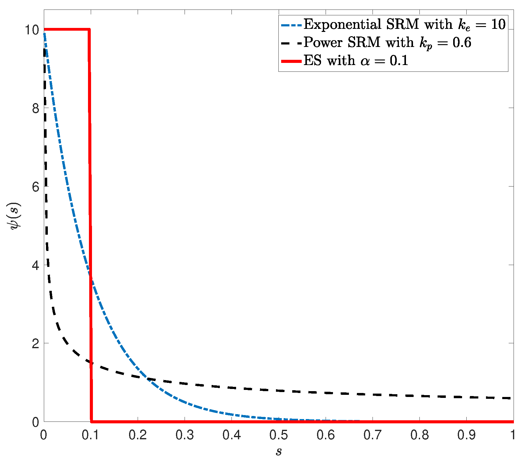
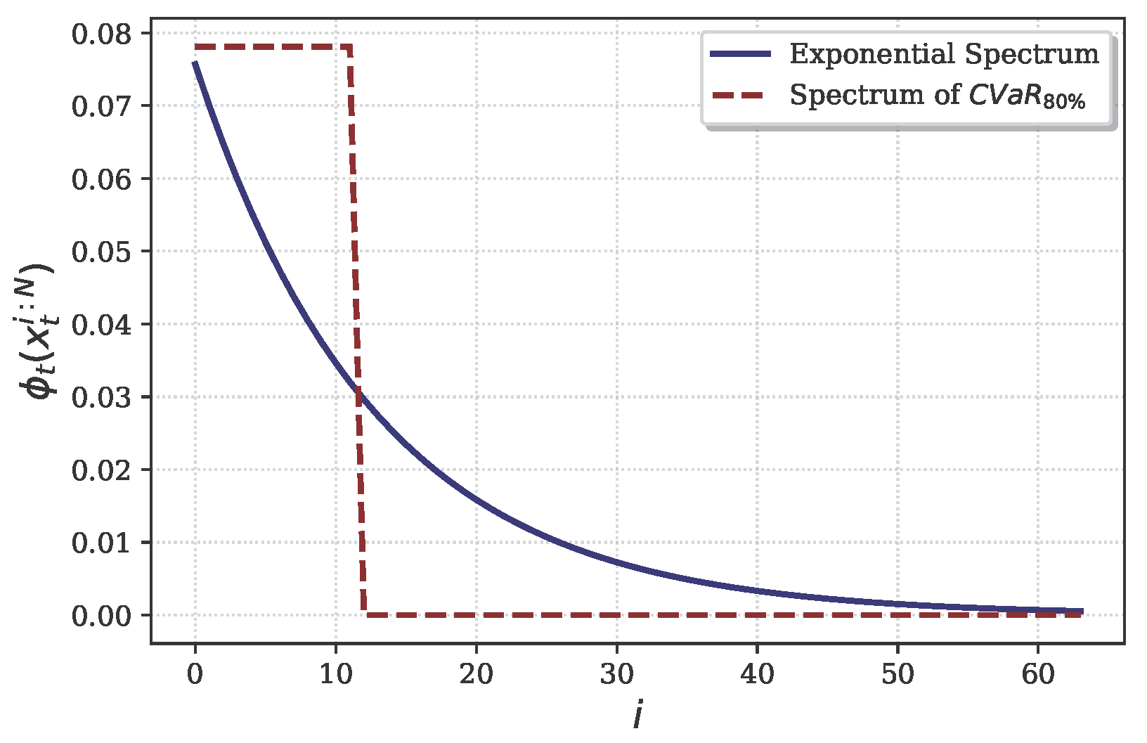
For the spectral risk measure, we employed an exponential spectrum defined as ${\varphi }_t(i)=(k_e·e^{-k_e·i})/(1-e^{-k_e})$, where $k_e=5$. This spectrum, illustrated in Figure 2, provides a nuanced representation of risk preferences across different probability levels, assigning greater weight to extreme losses. The function exhibits a high initial value for extreme losses and decreases exponentially as the loss magnitude diminishes, reflecting a risk-averse attitude. This configuration emphasizes severe, low-probability losses over more frequent, moderate ones. For comparison, we also plotted the CVaR spectrum with an $80\%$ quantile, represented by a step function in Figure 2. While CVaR assigns uniform weight to the worst $20\%$ of outcomes and zero to others, our exponential spectrum offers a more gradual transition. This approach facilitates a comprehensive risk assessment across all potential outcomes while maintaining an emphasis on tail risk.

We solved this optimization problem using the Progressive Hedging Algorithm, which was implemented with a step size of $r=1$ for updating dual variables, a maximum of 200 iterations, and a convergence tolerance of ${10}^{-2}$. Two distinct weighting schemes for the spectral risk measures and variance terms were explored to evaluate their impact on portfolio performance.

We compare the performance of two distinct weighting schemes: an intertemporal scheme that considers risk (SRM and variance) across all time periods and a terminal scheme that focuses solely on the risk at the final period. The first scheme, referred to as the “intertemporal weights” scheme, assigns equal importance to all time periods, setting ${\mu }_t=1$ and ${\kappa }_t=50$ for each $t\in \{1,2,3\}$. The second scheme, referred to as the “terminal weights” scheme, focuses exclusively on the final period by setting ${\mu }_T=1$ and ${\kappa }_T=50$, while nullifying the weights for intermediate periods (${\mu }_t={\kappa }_t=0$ for $t\in \{1,2\}$). The relatively large value of ${\kappa }_t$ compared to ${\mu }_t$ was chosen to balance the scales between the variance and SRM terms in the objective function, as the variance term tends to be smaller in magnitude than the SRM term.

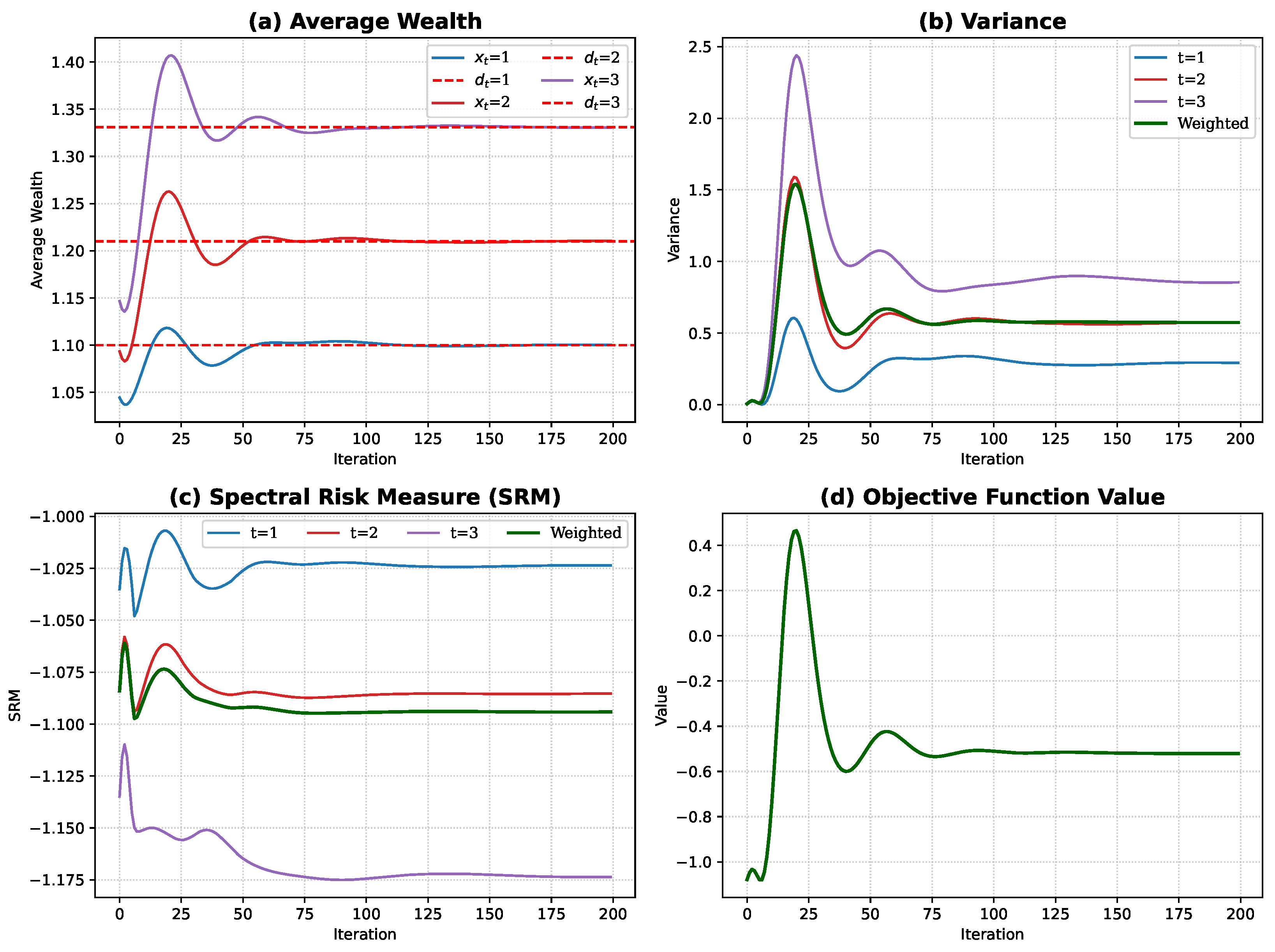
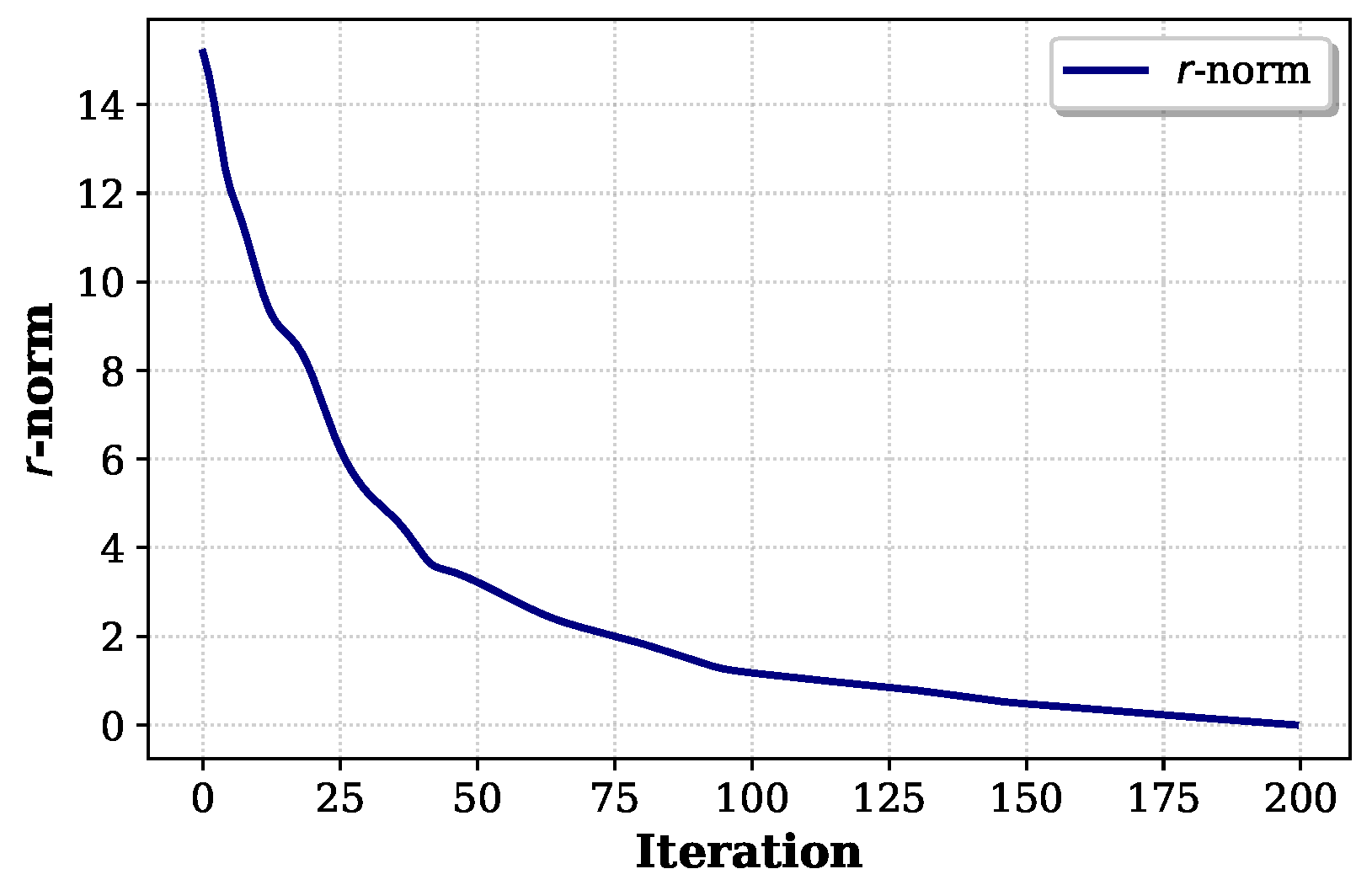
Figure 3 and Figure 4 demonstrate the convergence behavior of the PHA for intertemporal weighting schemes. Figure 3 tracks several performance metrics—average wealth, variance, SRM, and objective function value—which all stabilize after approximately 100 iterations. More importantly, Figure 4 shows the monotonic decrease in the r-norm, which measures the combined distance of primal and dual variables from their optimal values. The strictly decreasing pattern of the r-norm confirms the q-linear convergence rate established in Theorem 2. The empirical evidence of both the metric stabilization and the r-norm’s monotonic decrease validates the theoretical convergence properties of our modified PHA in solving the multi-period portfolio optimization problem with intertemporal risk measures.

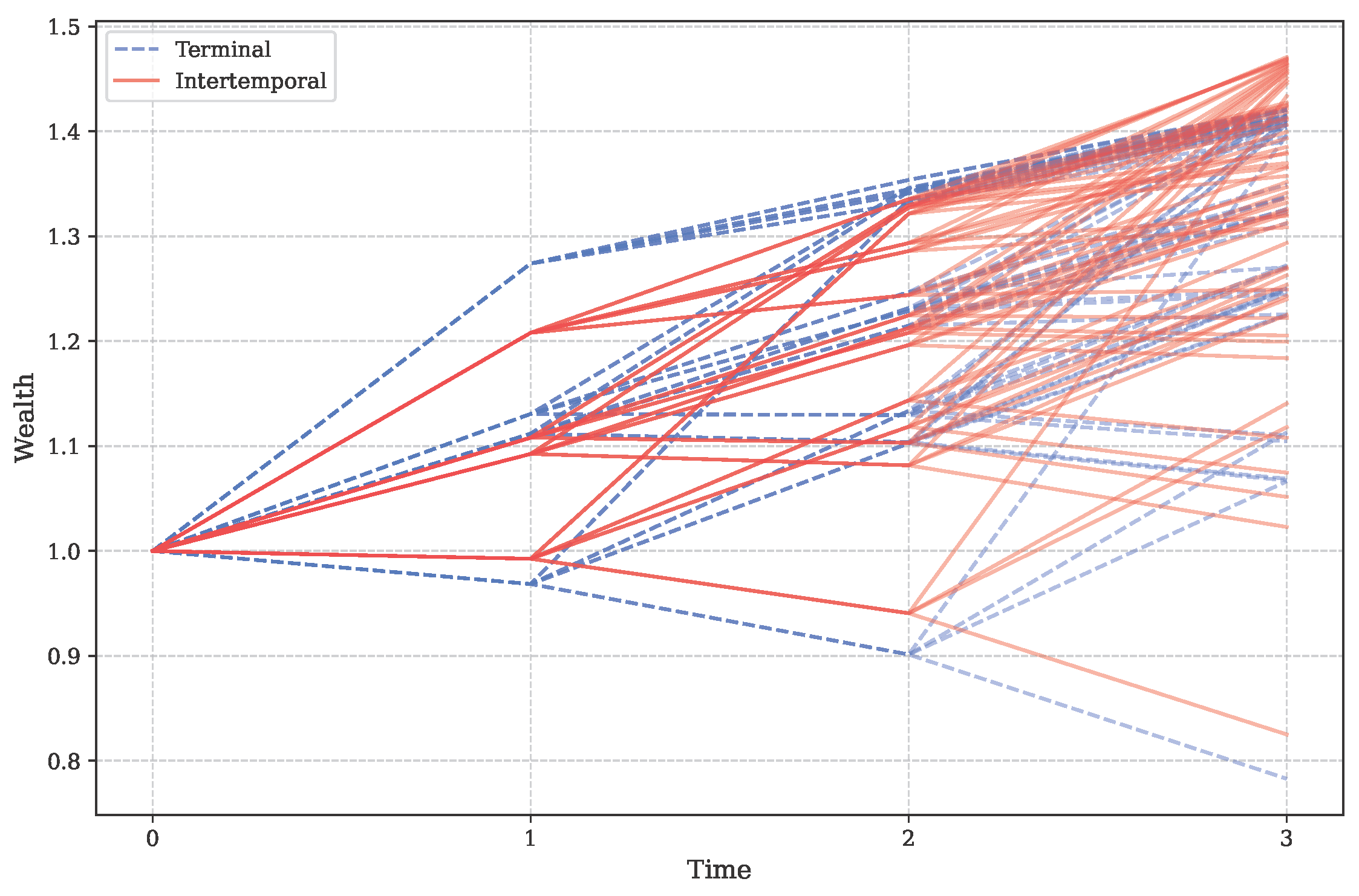
Figure 5 illustrates the wealth trajectories across all scenarios for both the intertemporal and terminal weighting schemes over the three-period investment horizon. The intertemporal scheme exhibits a tighter clustering of wealth trajectories, especially in the intermediate period ($t=1,2$). This tighter clustering suggests that the intertemporal approach provides more consistent wealth outcomes across different scenarios, indicating better risk management throughout the investment horizon. In contrast, the terminal weighting scheme shows a wider dispersion of wealth trajectories, particularly in the intermediate periods. This increased variability likely stems from the scheme’s focus on optimizing only the final period’s risk, allowing for greater fluctuations in earlier periods.

The observed tighter clustering of wealth trajectories under the intertemporal scheme (Figure 5), suggesting more consistent wealth outcomes, aligns with findings in other dynamic asset allocation studies, where strategies considering intermediate performance often lead to reduced path diversity and smoother wealth accumulation. For instance, [24] noted that incorporating intermediate variance controls in a multi-period setting, albeit with different risk measures, helped stabilize portfolio performance across scenarios.

While the trajectory plots offer a useful visual comparison, a more rigorous evaluation requires examining quantitative performance and risk metrics. More measure metrics are shown in

Table 1. Comparison of intertemporal and terminal metrics. OBJ stands for objective function value, WSRM stands for weighted SRM, and WVar stands for weighted variance.

Metric	OBJ	WSRM	WVar	Variance			SRM
				$\mathit{t}=\mathbf{1}$	$\mathit{t}=\mathbf{2}$	$\mathit{t}=\mathbf{3}$	$\mathit{t}=\mathbf{1}$	$\mathit{t}=\mathbf{2}$	$\mathit{t}=\mathbf{3}$
intertemporal	−0.5209	−1.0941	0.5733	0.0058	0.0115	0.0171	−1.0236	−1.0853	−1.1736
terminal	−0.3815	−1.0931	0.7116	0.0117	0.0155	0.0154	−1.0127	−1.0850	−1.1817
Metric	Skewness			Kurtosis			VaR
	$t=1$	$t=2$	$t=3$	$t=1$	$t=2$	$t=3$	$t=1$	$t=2$	$t=3$
intertemporal	0.0000	−0.8335	−1.3775	−1.0205	0.1556	2.1985	−0.9926	−0.9618	−1.0796
terminal	0.0000	−1.0297	−1.9513	−1.0151	0.5171	4.4911	−0.9685	−0.9315	−1.0742
Metric	Sharpe Ratio			Sortino Ratio			Omega Ratio
	$t=1$	$t=2$	$t=3$	$t=1$	$t=2$	$t=3$	$t=1$	$t=2$	$t=3$
intertemporal	0.6585	1.4966	2.1477	1.7513	5.8666	9.9094	4.5027	24.4664	72.2525
terminal	0.6585	1.4485	2.2610	1.7488	4.8562	8.4150	4.4975	20.4249	68.3198

Note: Bold values indicate better metrics.

. The intertemporal weighting scheme outperforms the terminal scheme in terms of the overall objective function value. This suggests that considering risk across all time periods leads to a more optimal solution according to our defined criteria. The intertemporal approach also achieves better time-weighted SRM and time-weighted variance scores.

Looking at the time-specific metrics, we observe that the intertemporal scheme generally provides better risk management in the earlier periods ($t=1,2$) across various measures, including variance, SRM, skewness, kurtosis, and VaR. This is consistent with its design to consider risk throughout the investment horizon. The terminal scheme, however, shows slightly better performance in some metrics for the final period ($t=3$), such as variance and SRM, aligning with its focus on terminal risk.

In terms of risk-adjusted return measures, we consider three widely used ratios: the Sharpe ratio, the Sortino ratio, and the Omega ratio. The Sharpe ratio measures excess return per unit of total risk, providing a general measure of risk-adjusted performance. The Sortino ratio is similar but focuses on downside risk, penalizing only returns below a target threshold. The Omega ratio offers a comprehensive view by considering the entire return distribution, weighing potential gains against losses. In our analysis, the intertemporal scheme demonstrates superior performance in Sortino and Omega ratios across all time periods, indicating better downside risk management. The Sharpe ratios are comparable, with the intertemporal scheme showing an advantage in earlier periods and the terminal scheme slightly outperforming in the final period.

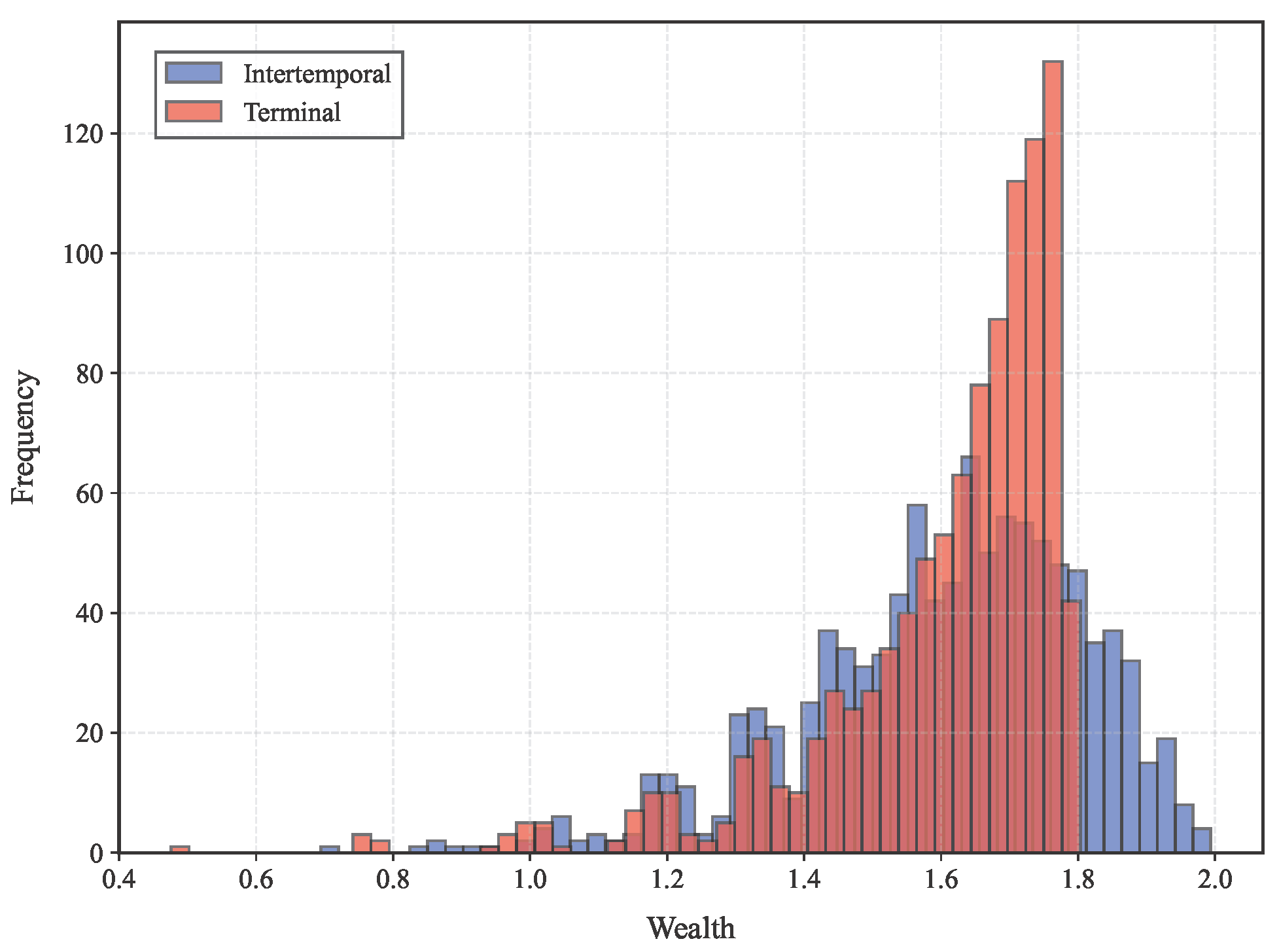
Moreover, we extend the time horizon to 5 periods, resulting in $4^5=1024$ scenarios. Figure 6 presents the distribution of terminal wealth under both the intertemporal and terminal schemes. The terminal scheme exhibits a leptokurtic (high-kurtosis) distribution with heavy tails, indicating a higher probability of extreme outcomes that may be undesirable for risk-averse investors. In contrast, the intertemporal scheme yields a more balanced wealth distribution with moderate tails and lower kurtosis, which better aligns with typical investor preferences for stable and predictable investment outcomes.

Overall, these results suggest that the intertemporal weighting scheme provides more consistent risk management across the entire investment horizon, leading to generally better performance metrics, especially in earlier periods. The terminal scheme, while focusing on and slightly outperforming in some final period metrics, appears to sacrifice some risk management in earlier periods.

5. Conclusions

This paper presents a comprehensive framework for multi-period portfolio optimization incorporating intertemporal spectral risk measures. Our approach makes several significant contributions to the literature on dynamic portfolio management and risk measurement.

First, we introduced a novel multi-period portfolio optimization model that integrates SRMs with variance measures across all time periods. This formulation fills an important gap by explicitly considering both types of risk in an intertemporal fashion. Second, we propose an efficient solution methodology based on a modified Progressive Hedging Algorithm, enhanced with specialized reformulations for handling linkage objectives and constraints.Third, our research provides strong theoretical underpinnings and empirical validation. We have established the q-linear convergence rate of our modified PHA under mild conditions, offering a solid theoretical foundation for its computational efficiency. Furthermore, comprehensive numerical experiments have validated the model’s effectiveness, demonstrating that an intertemporal focus on risk leads to superior downside risk protection—as evidenced by improved Sortino and Omega ratios—and more balanced terminal wealth distributions compared to traditional terminal-focused strategies.

The framework and findings of this research carry several practical implications for portfolio managers, institutional investors, financial advisors, and, potentially, financial regulators. The proposed model serves as a practical tool for investors to implement more sophisticated dynamic risk-management strategies. By considering both tail risk and volatility at each period, managers can better navigate uncertain market conditions and tailor strategies to achieve more consistent performance throughout the investment horizon, rather than focusing solely on terminal outcomes.

The ability to specify time-varying risk preferences via the spectral function allows investment strategies to be precisely aligned with evolving institutional needs or individual investor life-cycle considerations, such as a pension fund gradually de-risking its portfolio as it approaches its liability horizon.

Critically, our numerical results strongly suggest that incorporating ISRMs leads to better protection against significant losses, which is crucial for risk-averse investors, endowments, and any entity with strict drawdown limits or capital preservation mandates. Furthermore, many investors are concerned with performance and risk exposure during intermediate periods; our intertemporal approach directly addresses this by optimizing risk–return characteristics throughout the investment journey, leading to smoother wealth paths and increased confidence in meeting ongoing obligations. This allows for more informed decision-making in the design and management of complex financial products like structured products or target-date funds that require a nuanced approach to risk evolution.

In essence, our approach empowers investment professionals with a flexible and robust methodology to proactively manage multifaceted risks across time, leading to potentially more stable and desirable investment outcomes.

Moreover, the framework developed in this paper opens several promising directions for future research. These include the incorporation of transaction costs and market frictions, and the extension to robust optimization frameworks, for instance, to handle uncertainty in the spectral function itself. A crucial area for future investigation involves a comprehensive analysis of the model’s sensitivity to key assumptions—such as those related to market behavior and investor preferences—and its robustness under a wider range of market conditions. This could include evaluating alternative scenario generation methods that capture diverse market dynamics, and exploring the impact of varying investor preference parameters, like different spectral functions or risk aversion weights, or even extending to models where these preferences are endogenously determined or strategically designed [53]. Further research could also focus on adaptation to other complex market dynamics. Additionally, the methodological advances presented here may find applications beyond portfolio optimization, potentially benefiting other areas of financial risk management and dynamic decision-making under uncertainty.

In conclusion, our work provides both theoretical insights and practical tools for implementing dynamic risk-management strategies that effectively balance multiple objectives across time. The framework’s flexibility and computational tractability make it particularly valuable for institutional investors and asset managers seeking to implement sophisticated risk-management strategies in practice.

References

1. Markowitz, H.M. Portfolio Selection. J. Financ. 1952, 7, 1063–1070. [Google Scholar]
2. Artzner, P.; Delbaen, F.; Eber, J.M.; Heath, D. Coherent measure of risk. Math. Financ. 1999, 9, 203–228. [Google Scholar] [CrossRef]
3. Föllmer, H.; Schied, A. Convex measures od risk and trading contraints. Financ. Stoch. 2002, 6, 429–447. [Google Scholar] [CrossRef]
4. Kolm, P.N.; Tütüncü, R.; Fabozzi, F.J. 60 years of portfolio optimization: Practical challenges and current trends. Eur. J. Oper. Res. 2014, 234, 356–371. [Google Scholar] [CrossRef]
5. Gao, J.J.; Zhou, K.; Li, D.; Cao, X.R. Dynamic mean-LPM and mean-CVaR portfolio optimization in continuous-time. SIAM J. Control Optim. 2017, 55, 1377–1397. [Google Scholar] [CrossRef]
6. Zhou, K.; Gao, J.J.; Li, D.; Cui, X.Y. Dynamic mean-VaR portfolio selection in continuous time. Quant. Financ. 2017, 17, 1631–1643. [Google Scholar] [CrossRef]
7. He, X.D.; Zhou, X.Y. Dynamic portfolio choice when risk is measured by weighted VaR. Math. Oper. Res. 2015, 40, 773–796. [Google Scholar] [CrossRef]
8. Ortobelli, S.; Rachev, S.; Stoyanov, S.; Fabozzi, F.; Biglova, A. The proper use of risk measures in portfolio theory. Int. J. Theor. Appl. Financ. 2008, 8, 1107–1133. [Google Scholar] [CrossRef]
9. Adam, A.; Houkari, M.; Laurent, J.P. Spectral risk measures and portfolio selection. J. Bank. Financ. 2008, 32, 1870–1882. [Google Scholar] [CrossRef]
10. Steuer, R.E.; Na, P. Multiple criteria decison making combined with finance: A categorized bibliographic study. Eur. J. Oper. Res. 2003, 150, 496–515. [Google Scholar] [CrossRef]
11. Roman, D.; Mitra, G. Portfolio selection models: A review and new directions. Wilmott J. 2009, 1, 69–85. [Google Scholar] [CrossRef]
12. Wong, K.C.; Yam, S.C.P.; Zeng, J. Mean-risk portfolio management with bankruptcy prohibition. Insur. Math. Econ. 2019, 85, 153–172. [Google Scholar] [CrossRef]
13. Liu, H.Y.; Mao, T.T. Distributionally robust reinsurance with Value-at-Risk and Conditional Value-at-Risk. Insur. Math. Econ. 2022, 107, 393–417. [Google Scholar] [CrossRef]
14. Mi, H.; Xu, Z.Q. Optimal portfolio selection with VaR and portfolio insurance constraints under rank-dependent expected utility theory. Insur. Math. Econ. 2023, 110, 82–105. [Google Scholar] [CrossRef]
15. Gao, J.J.; Xiong, Y.; Li, D. Dynamic mean-risk portfolio selection with multiple risk measures in continuous-Time. Eur. J. Oper. Res. 2016, 249, 647–656. [Google Scholar] [CrossRef]
16. Roman, D.; Darby-Dowman, K.; Mitra, G. Mean-risk models using two risk measures: A multi-objective approach. Quant. Financ. 2007, 7, 443–458. [Google Scholar] [CrossRef]
17. Cesarone, F.; Martino, M.L.; Tardella, F. Mean-Variance-VaR portfolios: MIQP formulation and performance analysis. Spectr. 2023, 45, 1043–1069. [Google Scholar] [CrossRef]
18. Acerbi, C. Spectral measures of risk: A coherent representation of subjective risk aversion. J. Bank. Financ. 2002, 26, 1505–1518. [Google Scholar] [CrossRef]
19. Cai, J.; Li, J.Y.M.; Mao, T. Distributionally robust optimization under distorted expectations. Oper. Res. 2025, 73, 969–985. [Google Scholar] [CrossRef]
20. van Staden, P.M.; Dang, D.M.; Forsyth, P.A. On the distribution of terminal wealth under dynamic mean-variance optimal investment strategies. SIAM J. Financ. Math. 2021, 12. [Google Scholar] [CrossRef]
21. Costa, O.L.V.; Nabholz, R.B. Multiperiod Mean-Variance Optimization with Intertemporal Restrictions. J. Optim. Theory Appl. 2007, 134, 257–274. [Google Scholar] [CrossRef]
22. Li, D.; Ng, W.L. Optimal dynamic portfolio selection: Multiperiod mean-variance formulation. Math. Financ. 2000, 10, 387–406. [Google Scholar] [CrossRef]
23. Cui, X.Y.; Li, X.; Li, D. Unified Framework of Mean-Field Formulations for Optimal Multi-Period Mean-Variance Portfolio Selection. IEEE Trans. Autom. Control 2014, 59, 1833–1844. [Google Scholar] [CrossRef]
24. Wu, W.; Yu, D.; Wang, T.; Gao, J. Multiperiod mean-variance portfolio selection with intertemporal restrictions and correlated returns. In Proceedings of the 2018 Chinese Control and Decision Conference (CCDC), Shenyang, China, 9–11 June 2018; IEEE: Piscataway, NJ, USA, 2018; pp. 2347–2352. [Google Scholar]
25. Pan, Q.; Lin, Y.; Wu, J.; Zhong, J. Intertemporal constrained portfolio optimization problem with tracking-error. Appl. Math. Sci. Eng. 2025, 33, 2463456. [Google Scholar] [CrossRef]
26. Rockafellar, R.T.; Uryasev, S. Optimization of conditional value-at-risk. J. Risk 2000, 2, 21–41. [Google Scholar] [CrossRef]
27. Utz, S.; Wimmer, M.; Hirschberger, M.; Steuer, R.E. Tri-criterion inverse portfolio optimization with application to socially responsible mutual funds. Eur. J. Oper. Res. 2014, 234, 491–498. [Google Scholar] [CrossRef]
28. Basak, S.; Shapiro, A. Value-at-risk-based risk management: Optimal policies and asset prices. Rev. Financ. Stud. 2001, 14, 371–405. [Google Scholar] [CrossRef]
29. Bensoussan, A.; Hoe, S.R.; Kim, J.; Yan, Z.F. A risk extended version of Merton’s optimal consumption and portfolio selection. Eur. J. Oper. Res. 2022, 70, 815–829. [Google Scholar] [CrossRef]
30. Chiu, M.C.; Wong, H.Y.; Zhao, J. Dynamic safety first expected utility model. Eur. J. Oper. Res. 2018, 271, 141–154. [Google Scholar] [CrossRef]
31. Abad, C.; Iyengar, G. Portfolio Selection with Multiple Spectral Risk Constraints. SIAM J. Financ. Math. 2015, 6, 467–486. [Google Scholar] [CrossRef]
32. Guo, S.Y.; Xu, H.F. Robust spectral risk optimization when the subjective riskaversion is ambiguous: A moment-type approach. Math. Program. 2022, 194, 305–340. [Google Scholar] [CrossRef]
33. Moghimi, M.; Ku, H. Beyond CVaR: Leveraging Static Spectral Risk Measures for Enhanced Decision-Making in Distributional Reinforcement Learning. arXiv 2025, arXiv:2501.02087. [Google Scholar]
34. Chiu, M.C.; Wong, H.Y.; Li, D. Roy’s safety-first portfolio principle in financial risk management of disastrous events. Risk Anal. 2012, 32, 1856–1872. [Google Scholar] [CrossRef] [PubMed]
35. Madan, D.; Pistorius, M.; Stadje, M. On dynamic spectral risk measures, a limit theorem and optimal portfolio allocation. Financ. Stoch. 2017, 21, 1073–1102. [Google Scholar] [CrossRef]
36. Rockafellar, R.T.; Wets, R.J.B. Scenarios and policy aggregation in optimization under uncertainty. Math. Oper. Res. 1991, 16, 119–147. [Google Scholar] [CrossRef]
37. Watson, J.P.; Woodruff, D.L. Progressive hedging innovations for a class of stochastic mixed-integer resource allocation problems. Comput. Manag. Sci. 2011, 8, 355–370. [Google Scholar] [CrossRef]
38. Carpentier, P.L.; Gendreau, M.; Bastin, F. Long-term management of a hydroelectric multireservoir system under uncertainty using the progressive hedging algorithm. Water Resour. Res. 2013, 49, 2812–2827. [Google Scholar] [CrossRef]
39. Gul, S.; Denton, B.T.; Fowler, J.W. A progressive hedging approach for surgery planning under uncertainty. INFORMS J. Comput. 2015, 27, 755–772. [Google Scholar] [CrossRef]
40. Hvattum, L.M.; Løkketangen, A. Using scenario trees and progressive hedging for stochastic inventory routing problems. J. Heuristics 2009, 15, 527–557. [Google Scholar] [CrossRef]
41. Crainic, T.G.; Fu, X.; Gendreau, M.; Rei, W.; Wallace, S.W. Progressive hedging-based metaheuristics for stochastic network design. Networks 2011, 58, 114–124. [Google Scholar] [CrossRef]
42. Rockafellar, R.T. Solving stochastic programming problems with risk measures by progressive hedging. Set-Valued Var. Anal. 2018, 26, 759–768. [Google Scholar] [CrossRef]
43. Jin, C.; Wu, W.; Xie, J. Responsible Investing: A Multi-Period Portfolio Selection Model. 2024. Available online: https://ssrn.com/abstract=4814019 (accessed on 21 May 2025).
44. Kusuoka, S. On Law Invariant Coherent Risk Measures; Advances in mathematical economics; Springer: Tokyo, Japan, 2001; pp. 83–95. [Google Scholar]
45. Brandtner, M. ”Spectral Risk Measures: Properties and Limitation”: Comment on Dowd, Cotter, and Sorwar. J. Financ. Serv. Res. 2016, 49, 121–131. [Google Scholar] [CrossRef]
46. Bertsimas, D.; Lasuprete, G.J.; Samarov, A. Shortfall as a risk measure: Properties, optimization and applications. J. Econ. Dyn. Control 2004, 28, 1353–1381. [Google Scholar] [CrossRef]
47. Dowd, K.; Cotter, J.; Sorwar, G. Spectral Risk Measures: Properties and Limitations. J. Financ. Serv. Res. 2008, 34, 61–75. [Google Scholar] [CrossRef]
48. Brandtner, M. Conditional Value-at-Risk, spectral risk measures and (non-) diversification in portfolio selection problems-A comparison with mean-variance analysis. J. Bank. Financ. 2013, 37, 5526–5537. [Google Scholar] [CrossRef]
49. Strub, M.S.; Li, D.; Cui, X.; Gao, J. Discrete-time mean-CVaR portfolio selection and time-consistency induced term structure of the CVaR. J. Econ. Dyn. Control 2019, 108, 103751. [Google Scholar] [CrossRef]
50. Cui, X.; Gao, J.; Shi, Y.; Zhu, S. Time-consistent and self-coordination strategies for multi-period mean-conditional value-at-risk portfolio selection. Eur. J. Oper. Res. 2019, 276, 781–789. [Google Scholar] [CrossRef]
51. Acerbi, C.; Simonetti, P. Portfolio optimization with spectral measure of risk. arXiv 2002, arXiv:cond-mat/0203607. [Google Scholar]
52. Benati, S.; Rizzi, R. A mixed integer linear programming formulation of the optimal mean/value-at-risk portfolio problem. Eur. J. Oper. Res. 2007, 176, 423–434. [Google Scholar] [CrossRef]
53. Liu, S.; Zhu, Q. Stackelberg risk preference design. Math. Program. 2025, 209, 785–823. [Google Scholar] [CrossRef]
Figure 1. The spectrum function ϕ t ( s ) in the spectral risk measure.
Mathematics 13 01754 g001
Figure 2. Comparison of exponential spectrum ( k e = 5 ) and spectrum of CVaR (80% quantile) used in the SRM. The exponential spectrum provides a more gradual weighting of risk across probability levels compared to the step function of CVaR.
Mathematics 13 01754 g002
Figure 3. Convergence of average wealth, variance, SRM, and objective value over iterations for the terminal weighting scheme.
Mathematics 13 01754 g003
Figure 4. Convergence of the r-norm over iterations, demonstrating the q-linear convergence rate of the modified PHA. The r-norm measures the combined distance of primal and dual variables from their optimal values.
Mathematics 13 01754 g004
Figure 5. Wealth trajectories across all scenarios for intertemporal and terminal weighting schemes over the investment horizon. The intertemporal scheme exhibits tighter clustering of wealth outcomes, particularly in intermediate periods, indicating more consistent risk management throughout the investment horizon.
Mathematics 13 01754 g005
Figure 6. Distribution of terminal wealth under intertemporal and terminal schemes over a 5-period horizon. The terminal scheme exhibits a leptokurtic distribution with heavy tails, while the intertemporal scheme shows a more moderate distribution pattern.
Mathematics 13 01754 g006