Unsupervised Attribute Reduction Algorithms for Multiset-Valued Data Based on Uncertainty Measurement

Abstract

Missing data introduce uncertainty in data mining, but existing set-valued approaches ignore frequency information. We propose unsupervised attribute reduction algorithms for multiset-valued data to address this gap. First, we define a multiset-valued information system (MSVIS) and establish $\theta$-tolerance relation to form the information granules. Then, $\theta$-information entropy and $\theta$-information amount are introduced as uncertainty measures. Finally, these two UMs are used to design two unsupervised attribute reduction algorithms in an MSVIS. The experimental results demonstrate the superiority of the proposed algorithms, achieving average reductions of 50% in attribute subsets while improving clustering accuracy and outlier detection performance. Parameter analysis further validates the robustness of the framework under varying missing rates.

1. Introduction

1.1. Research Background

Data with missing information values, also called missing data, are a common occurrence in datasets for various reasons. Simple approaches like listwise deletion handle missing data by removing incomplete records. Despite their simplicity, such methods risk losing valuable information and introducing bias. Moreover, it could result in bias sometimes [1]. Data imputation is a statistical method that fills the missing values by applying reasonable rules. Common imputation techniques include mean substitution and regression imputation [1]. Despite their utility, imputation methods also carry the risk of inducing bias [2].

On the other hand, mathematical models such granular computing (GrC) [3] and rough set theory (RST) [4] are effective tools for dealing with uncertainty. GrC is a significant methodology in artificial intelligence. It has its unique theory, which tries to obtain a granular structure representation of a problem. Providing a basic conceptual framework, GrC is broadly researched in pattern recognition [5] and data mining [6]. As a realistic approach of GrC, RST provides a mathematical tool to handle uncertainty, such as imprecision, inconsistency, and incomplete information [7,8]. An information system (IS) was also presented by Pawlak [4]. The vast majority of applications of RST are bound with an IS.

In RST, a dataset with missing information values is usually represented by an incomplete information system (IIS). An SVIS represents each missing information value under an attribute with all possible values, and each information value that is not missing with a set of its original value. Thus, an SVIS can be obtained from an IIS. As an effective way of handling missing information values, SVIS has drawn great attention from researchers. For instance, Chen et al. [9] investigated the attribute reduction of an SVIS based on a tolerance relation. Dai et al. [8] investigated UMs in an SVIS. Furthermore, an SVIS with missing information values is also studied. Xie et al. [10] investigated the UMs for an incomplete probability SVIS. Chen et al. [11] presented UMs for an incomplete SVIS by using Gaussian kernel.

Feature selection, also known as attribute reduction in RST, is used to reduce redundant attributes and the complexity of calculation for high-dimensional data while improving or maintaining the algorithm performance of a particular task. UM holds particular relevance in the context of attribute reduction within an information system. Zhang et al. [12] investigated UM for categorical data using fuzzy information structures and applied it to attribute reduction. Gao et al. [13] studied a monotonic UM for attribute reduction based on granular maximum decision entropy.

An SVIS is a valuable tool for handling datasets with missing information values. Specifically, an SVIS approach involves replacing the missing information values of an attribute with a set comprising all the possible values that could exist under the same attribute. Meanwhile, the existing information values are substituted with a set containing the original values. By employing this technique, a dataset containing missing information values can be converted into an SVIS, enabling the application of further processes such as calculating the Jaccard distance within the framework of an SVIS.

The study on attribute reduction in an SVIS are abundant. Just to name a few, Peng et al. [14] delved into uncertainty measurement-based feature selection for set-valued data. Singh et al. [15] explored attribute selection in an SVIS based on a fuzzy similarity. Zhang et al. [16] studied attribute reduction for set-valued data based on D-S evidence theory. Liu et al. [17] proposed an incremental attribute reduction method for set-valued decision information system with variable attribute sets. Lang et al. [18] studied an incremental approach to attribute reduction of a dynamic SVIS.

However, the straightforward replacement of missing information with all possible values in an SVIS can be considered overly simplistic and may result in some loss of information. This approach fails to consider the potential variations in the occurrence frequency of different attribute values, leading to a lack of differentiation between values that may occur more frequently than others and should thus be treated distinctively.

An MSVIS has been developed to enhance the functionality of an SVIS [19,20,21]. In the MSVIS framework, the information values associated with an attribute in a dataset are organized as multisets, which allow elements to be repeated. Within an MSVIS, each missing information value is represented by a multiset, ensuring that the frequency of each value is maintained. Information values that are not missing are depicted by multisets that are equivalent to traditional sets containing only the original value.

This approach enables an MSVIS to accurately capture the frequency distribution of information values within the dataset, addressing one of the limitations of an SVIS related to potential information loss arising from oversimplified imputation strategies. By preserving the frequency information associated with each value, an MSVIS provides a more nuanced representation of the dataset, enhancing the robustness and accuracy of data analysis processes.

Despite the benefits of an MSVIS, research on attribute reduction in an MSVIS is relatively scarce compared to the extensive body of research focused on an SVIS. Huang et al. [22] developed a supervised feature-selection method for multiset-valued data using fuzzy conditional information entropy, while Li et al. [23] proposed a semi-supervised approach to attribute reduction for partially labelled multiset-valued data.

Recent advancements in unsupervised attribute reduction have primarily focused on improving computational efficiency and scalability. For instance, Feng et al. [24] proposed a dynamic attribute reduction algorithm using relative neighborhood discernibility, achieving incremental updates for evolving datasets. While their method demonstrates efficiency in handling object additions, it neglects the critical role of frequency distributions in multiset-valued data: a gap that leads to information loss in scenarios like dynamic feature evolution or missing value imputation. Similarly, He et al. [25] introduced uncertainty measures for partially labeled categorical data, yet their semi-supervised framework still relies on partial labels and predefined thresholds, limiting applicability in fully unsupervised environments. Zonoozi et al. [26] proposed an unsupervised adversarial domain adaptation framework using variational auto-encoders (VAEs) to align feature distributions across domains. While it validates the robustness of domain-invariant feature learning, it neglects frequency semantics in missing data. Chen et al. [27] introduced an ensemble regression method that assigns weights to base models based on relative error rates. Although effective for continuous targets, their approach relies on predefined error metrics and ignores the intrinsic frequency distributions in multiset-valued data.

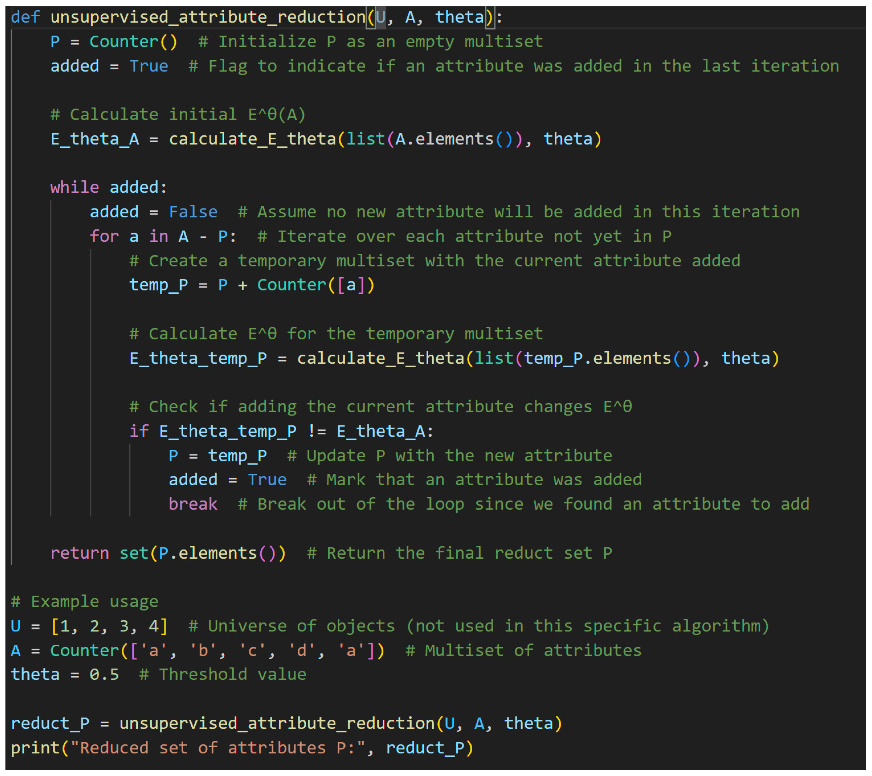
To bridge these gaps, we propose the multiset-valued information system (MSVIS) framework in unsupervised attribute reduction, which uniquely integrates frequency-sensitive uncertainty measurement for missing data with granular computing principles. Unlike conventional SVIS-based methods (e.g., uniform set imputation), an MSVIS explicitly preserves frequency distributions (e.g., 2/S,3/M) through multisets, enabling dynamic adjustments via $\theta$-tolerance relations. Building on this, this paper uses an MSVIS to represent a dataset with missing information values and builds a UM-based attribute reduction method within it.

$\left(1\right)$ Attribute reduction and missing data processing have been researched mainly as two separate data preprocess topics, and related work has been focused on attribute reduction in an SVIS. This paper combines them together, that is, the task of attribute reduction for missing data. The proposed method offers several advantages. Firstly, unlike some data imputation methods, it does not presume any data distribution and is totally based on data itself. Secondly, unlike the approaches proposed by Huang et al. [22] and Li et al. [23], which necessitate the presence of decision attributes in a dataset, the method introduced in this paper does not require decision attributes, thereby expanding its applicability across a broader range of datasets. Lastly, the method proposed in this paper is user-friendly and easy to implement, ensuring accessibility and facilitating its practical application in diverse research and application scenarios.

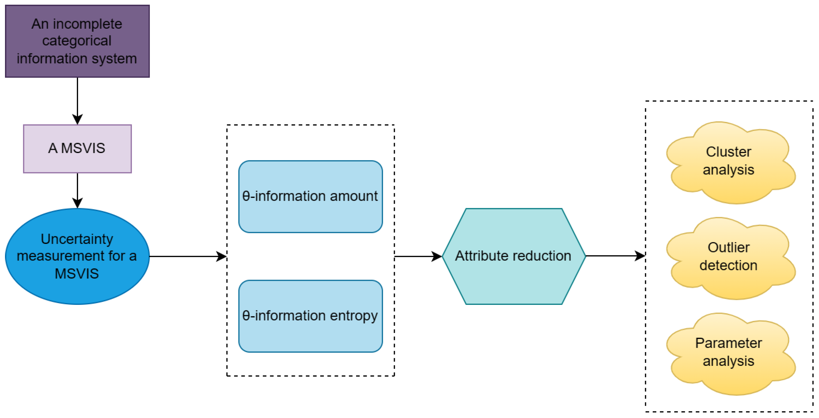
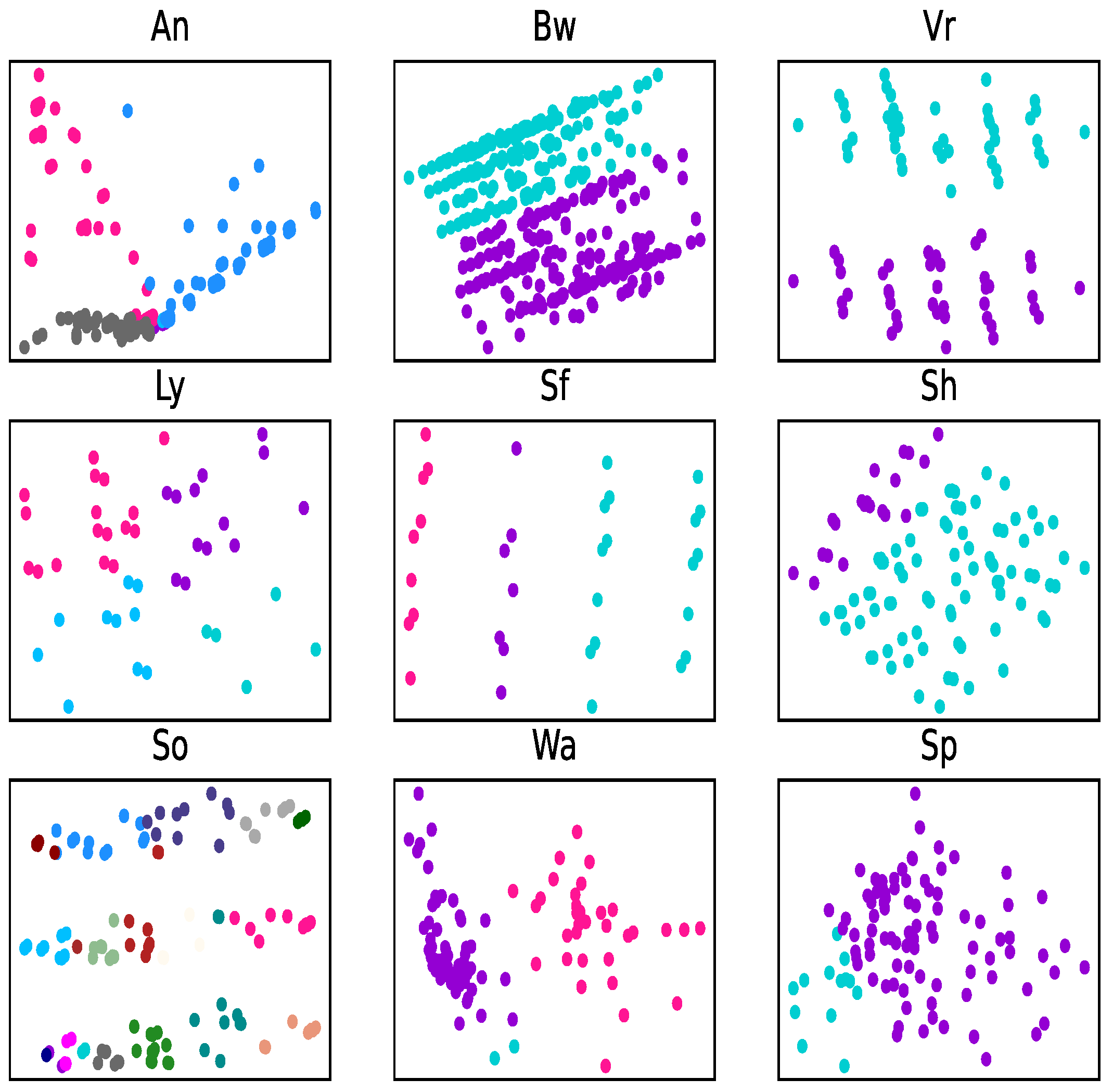
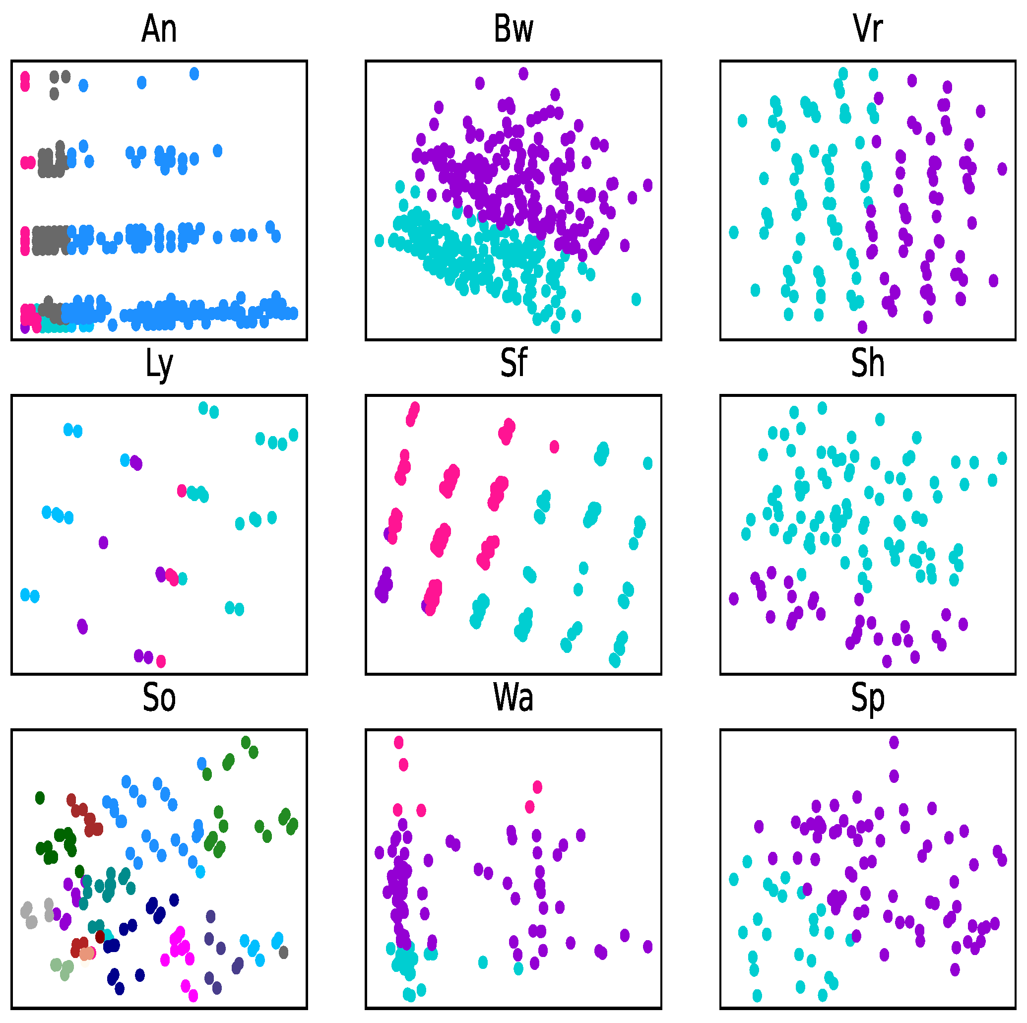
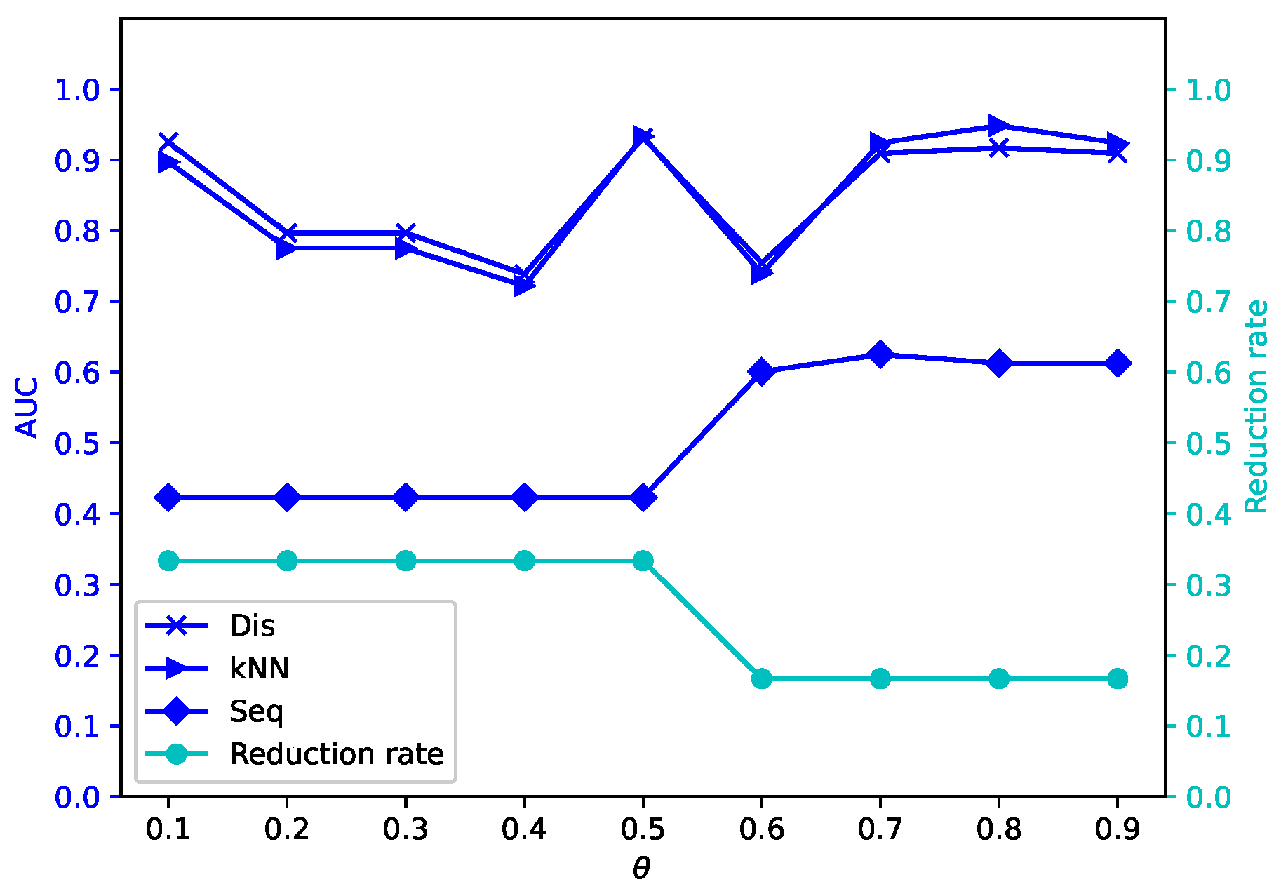
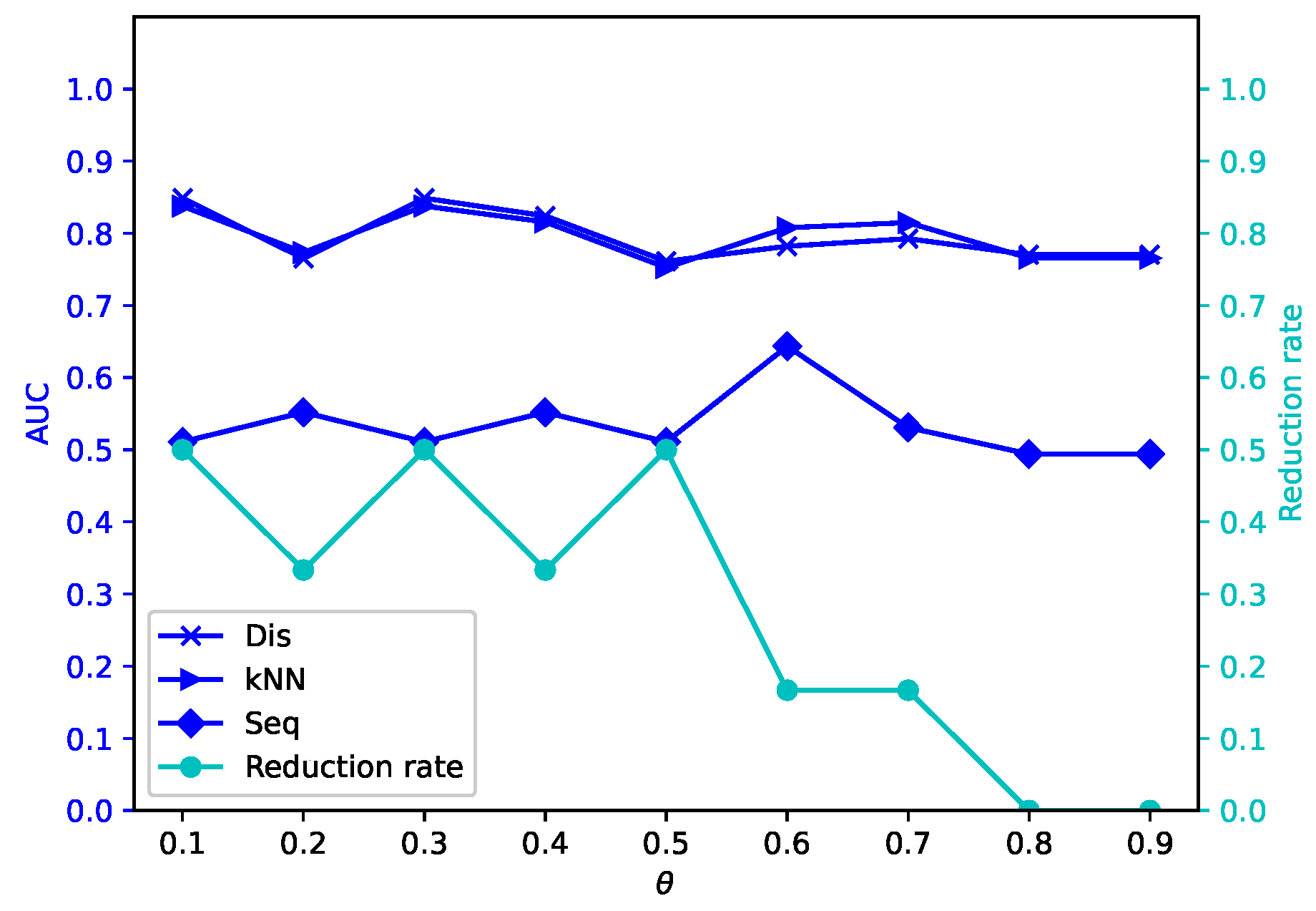
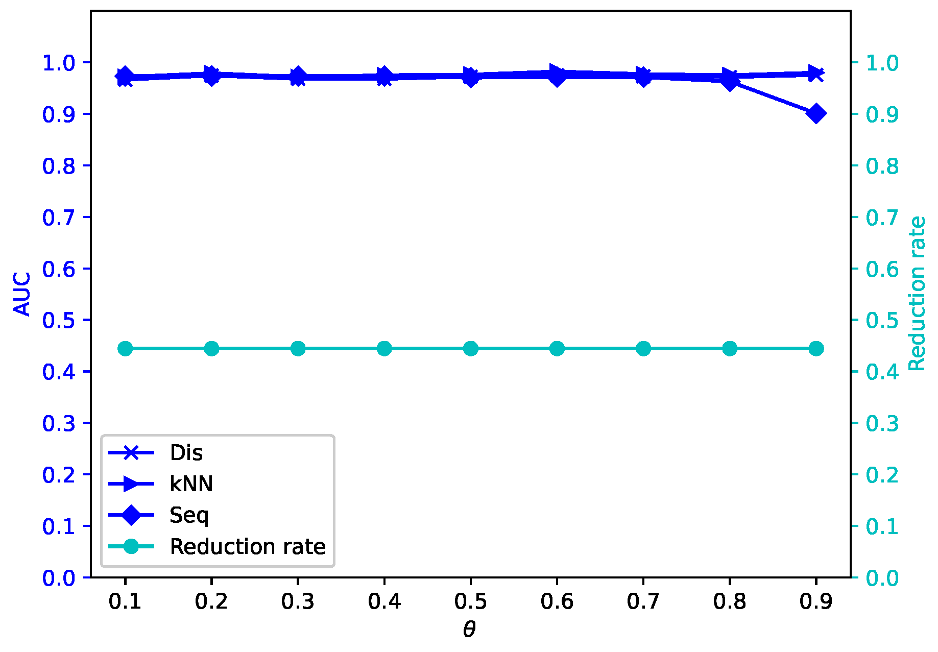
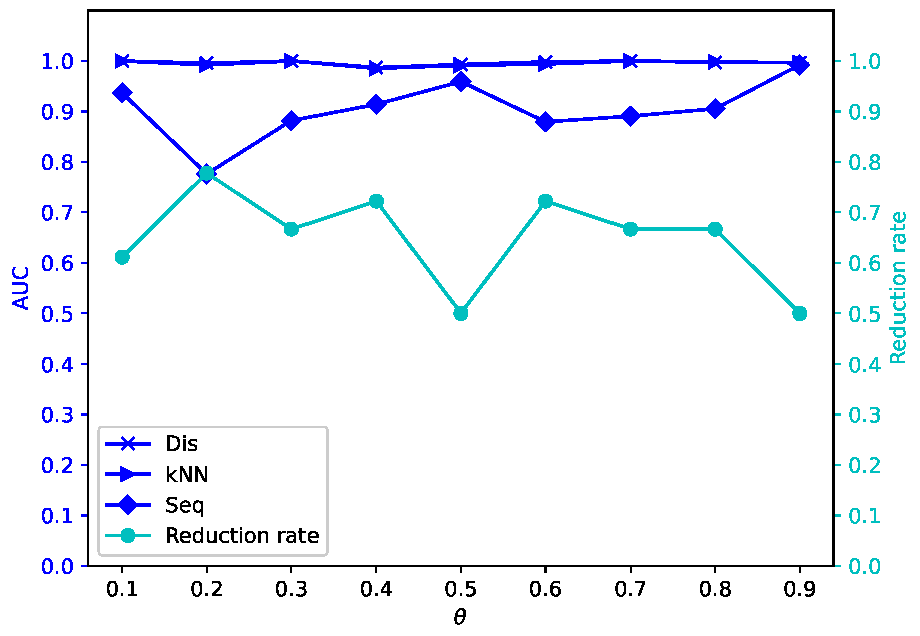
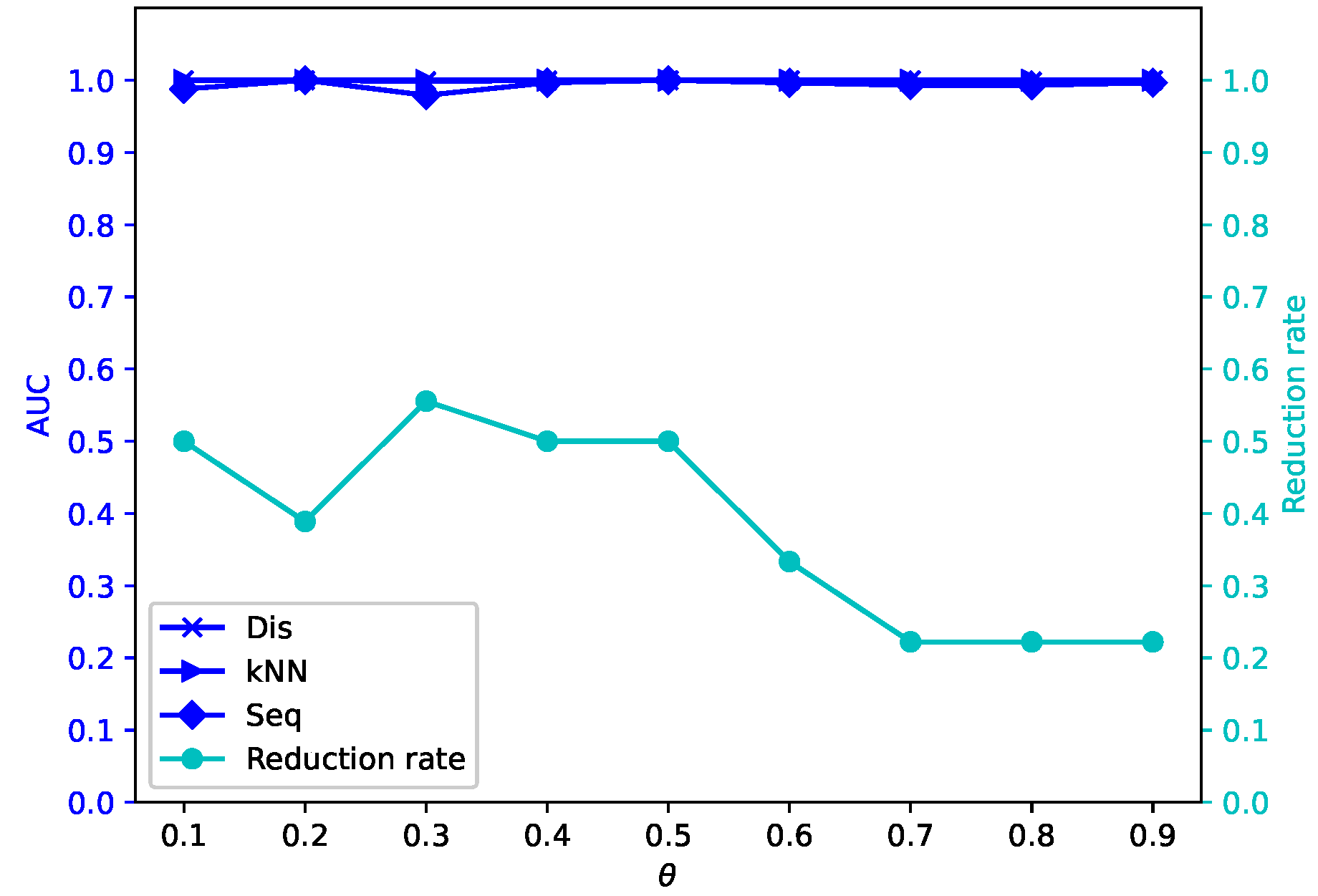
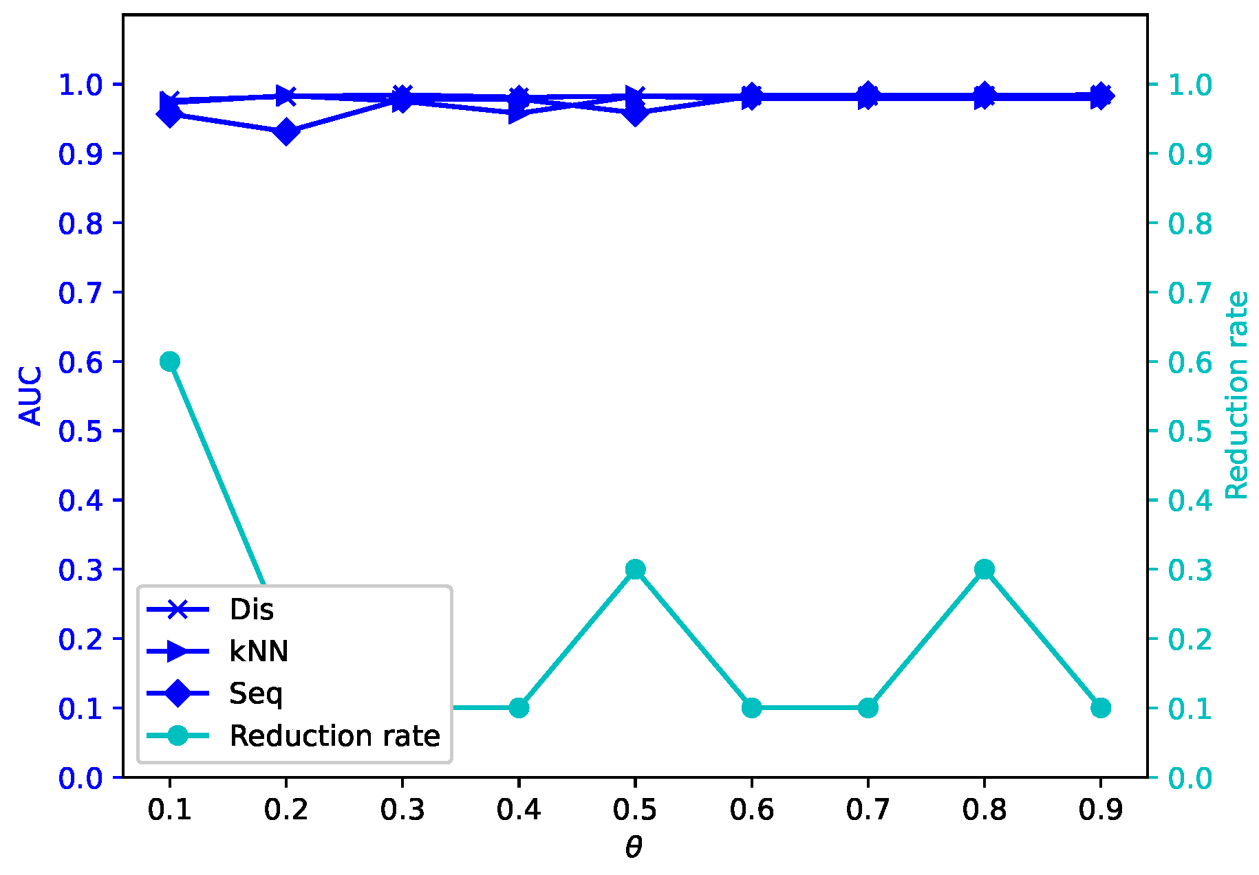
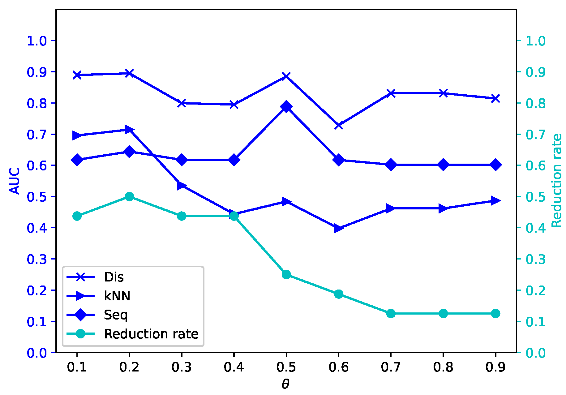
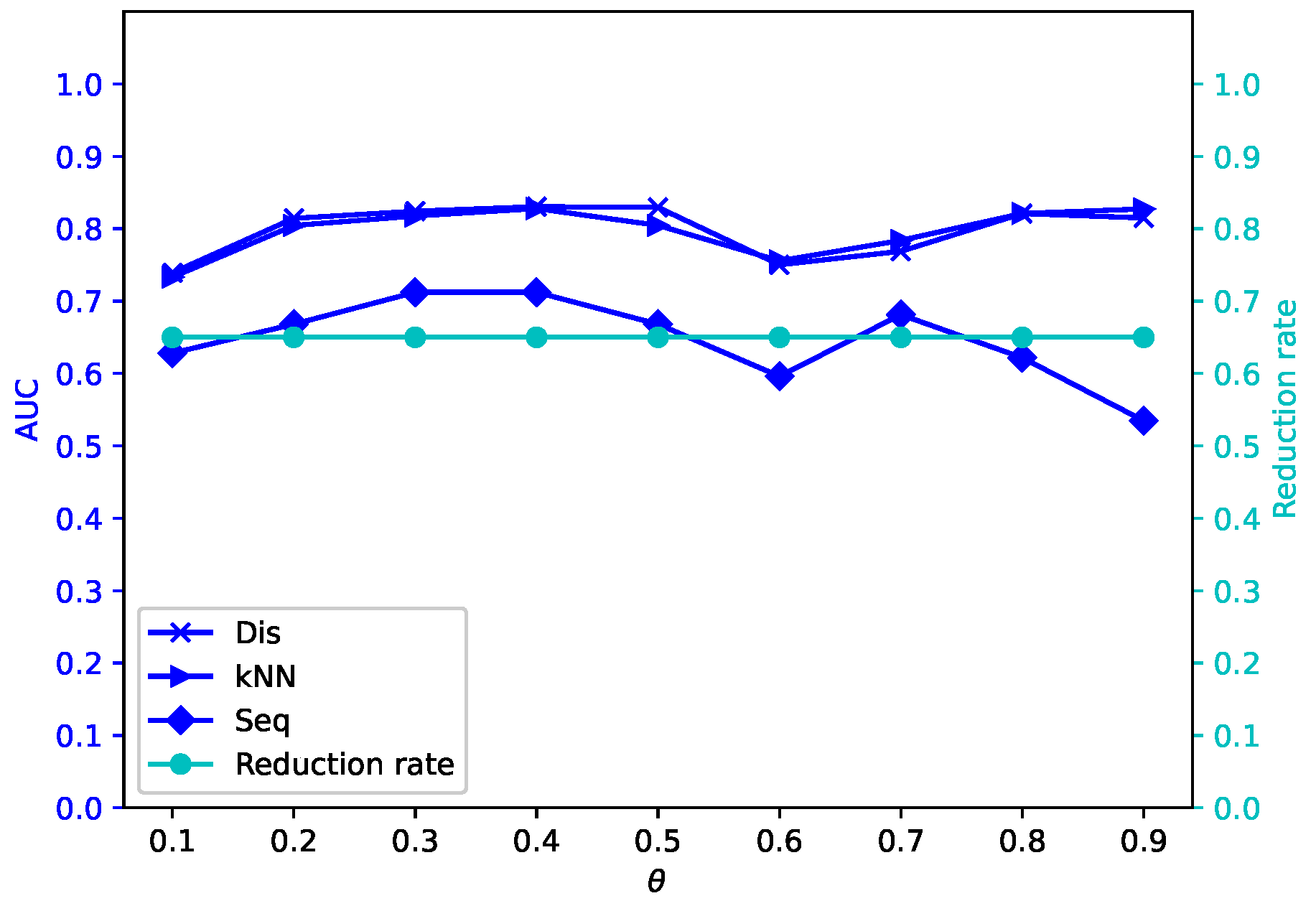
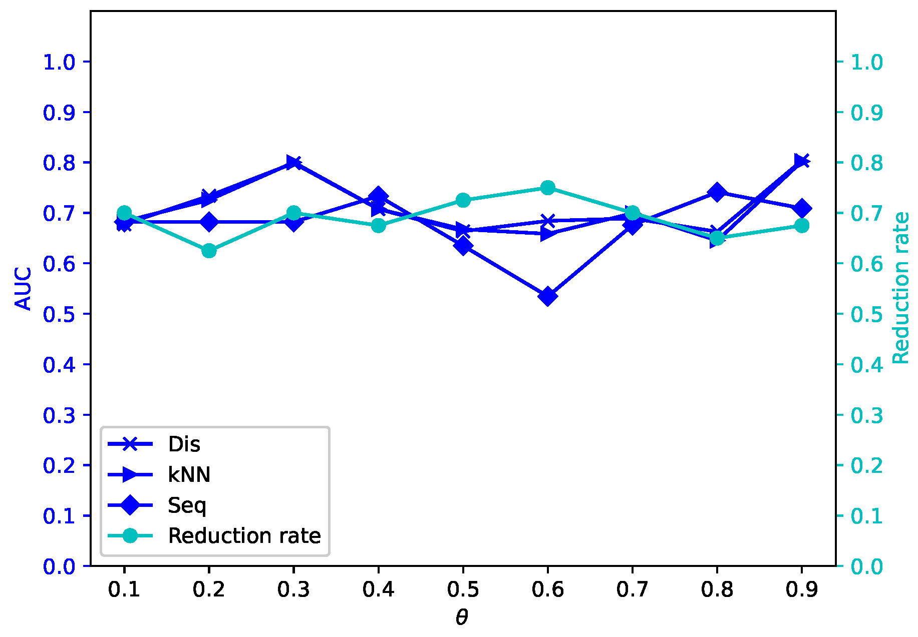
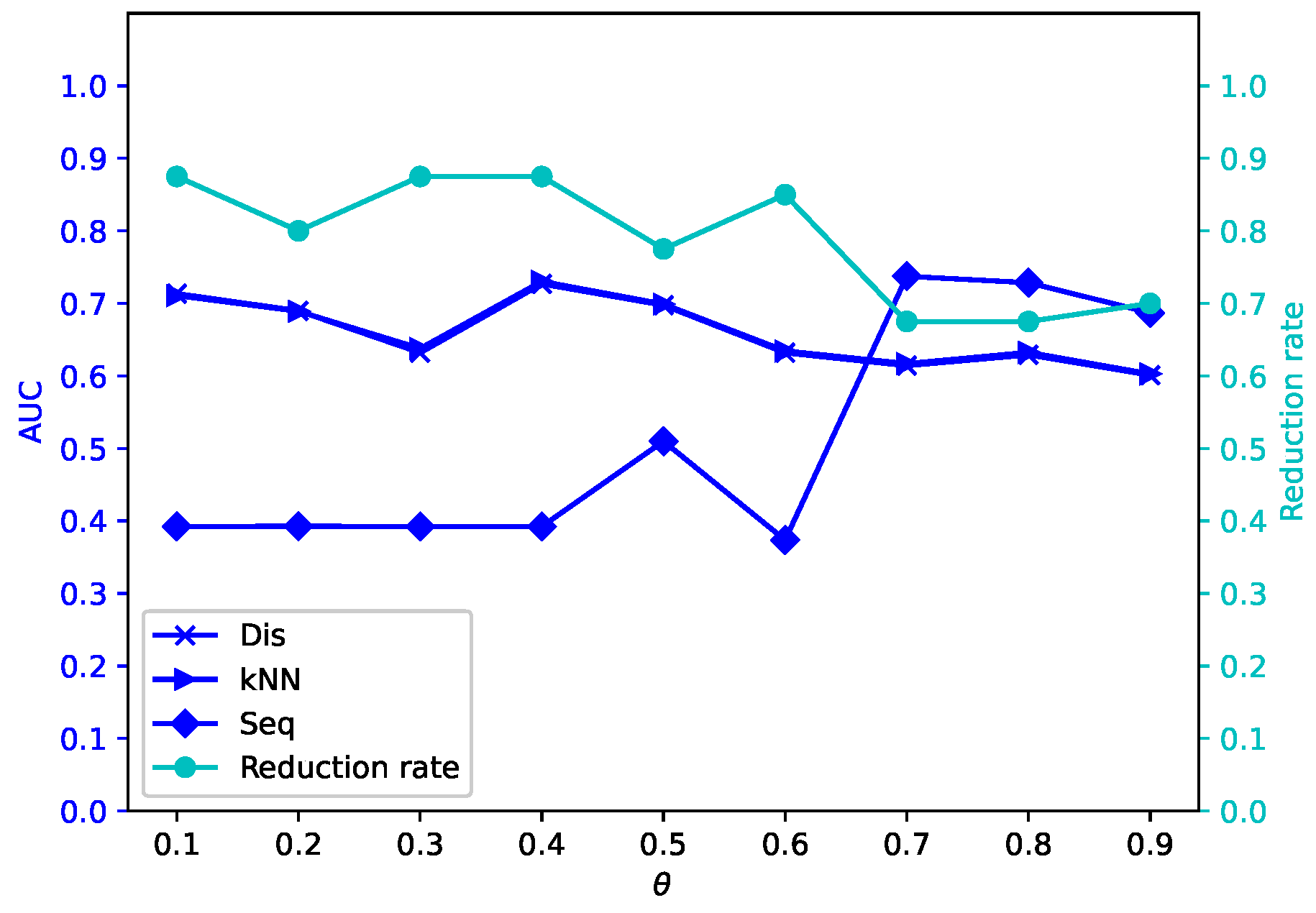
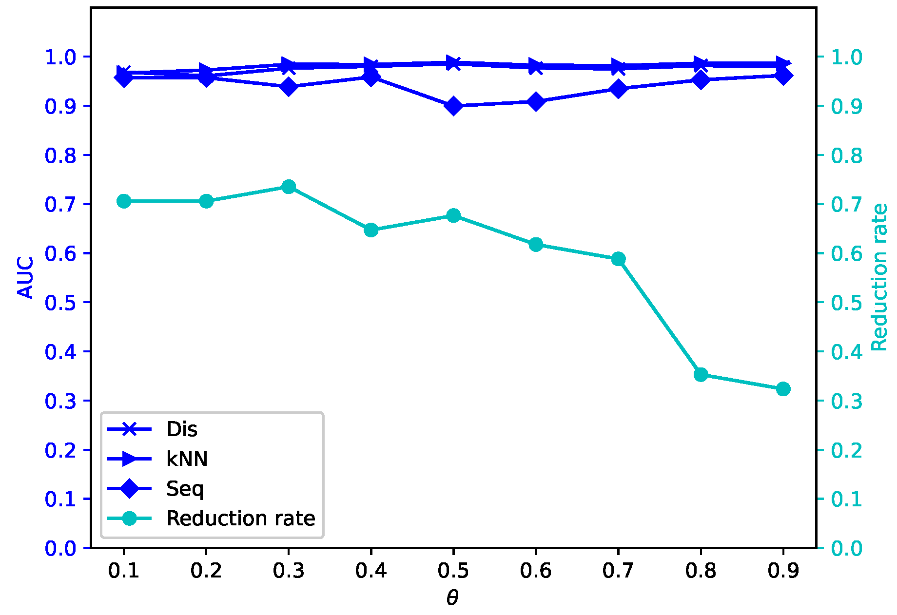
$\left(2\right)$ Different attribute reduction algorithms are compared. Particularly, the proposed attribute reduction algorithms are conducted in both MSVIS and SVIS and then are compared. Parameter analysis is also conducted to see the influence of the parameters. The experimental results show the effectiveness and superiority of the proposed algorithms.

1.2.  Organization

The structure of this paper is outlined as follows. Section 2 recalls multisets and rational probability distribution sets, and the one-to-one correspondence between them, as shown in Theorem 1. Section 3 shows that an IIS induces an MSVIS, and defines a $\theta$-tolerance relation with the help of Theorem 1. Section 4 presents two UMs based on the $\theta$-tolerance relation for an MSVIS. Section 5 proposes unsupervised attribute reduction algorithms based on the UMs. Section 6 carries out clustering analysis, outlier detection, and parameter analysis to show the effectiveness of the proposed algorithms. Section 7 concludes this paper.

Figure 1 depicts the structure of this paper.

2. Preliminaries

Let $U=\{u_1,u_2,\dots ,u_n\}$ be a finite object set. $2^U$ denotes a collection of all object subsets of U and $\left|X\right|$ means the cardinality of $X\in 2^U$. Put

$$\delta =U\times U,▵=\left\{\right(u,u):u\in U\}.$$

Definition 1

([28]). Given a non-empty finite set V, a multiset or bag M drawn from V can be defined by a count function $C_M$: $V\to N\cup \left\{0\right\}$.

For convenience,

$$M\left(v\right)isusedtodenote{C}_M\left(v\right)(v\in V).$$

$M\left(v\right)=m$ indicates that v occurs m times in the multiset M, which is denoted by $m/v\in M$ or $v{\in }^{m}M$.

Suppose $V=\{v_1,v_2,\dots ,v_s\}$; if  $M\left(v_i\right)=m_i(i=1,2,\dots ,s)$, then M is denoted by $\{m_1/v_1,m_2/v_2,\cdots ,m_s/v_s\}$, i.e.,

$$M=\{m_1/v_1,m_2/v_2,\dots ,m_s/v_s\}.$$

Definition 2

([28]). Consider a non-empty finite set V, and let M and N be two multisets drawn from V. The following definitions apply:

$\left(1\right)$$M=N⟺M\left(v\right)=N\left(v\right)(v\in V);$

$\left(2\right)$$M⊑N⟺M\left(v\right)\le N\left(v\right)(v\in V);$

$\left(3\right)$$P=M\bigsqcup N⟺P\left(v\right)=M\left(v\right)\vee N\left(v\right)(v\in V);$

$\left(4\right)$$P=M\sqcap N⟺P\left(v\right)=M\left(v\right)\wedge N\left(v\right)(v\in V).$

$\left(5\right)$$P=M\oplus N⟺P\left(v\right)=M\left(v\right)+N\left(v\right)(v\in V);$

$\left(6\right)$$P=M\ominus N⟺P\left(v\right)=\left(M\right(v)-N(v\left)\right)\vee 0(v\in V).$

Definition 3

([29]). Let $V=\{v_1,v_2,\dots ,v_s\}$ and $P=\left\{{\displaystyle \frac{v_1,v_2,\dots ,v_s}{p_1,p_2,\dots ,p_s}}\right\},$ P is called a probability distribution set over V, if $\forall i$, $0\le p_i\le 1$ and ${\displaystyle \sum _{i=1}^s}{p}_i=1,$

P could be represented as a mapping $P:V\to [0,1]$, $\forall i,P\left(v_i\right)=p_i$.

Definition 4

([19]). Let $V=\{v_1,v_2,\dots ,v_s\}$, and $P=\left\{{\displaystyle \frac{v_1,v_2,\dots ,v_s}{p_1,p_2,\dots ,p_s}}\right\}$ be a probability distribution set over V. If $\forall i$, $p_i$ is a rational number, P is referred to as a rational probability distribution set over V; otherwise, P is referred to as an irrational probability distribution set over V.

Definition 5

([29]). Let $V=\{v_1,v_2,\dots ,v_s\}$, and let

$$P=\left\{{\displaystyle \frac{v_1,v_2,\dots ,v_s}{p_1,p_2,\dots ,p_s}}\right\},Q=\left\{{\displaystyle \frac{v_1,v_2,\dots ,v_s}{q_1,q_2,\dots ,q_s}}\right\}$$

be two probability distribution sets overs V. The well-known Hellinger distance between P and Q is as follows

$$HD(P,Q)={\displaystyle \frac{1}{\sqrt{2}}}\sqrt{\sum _{i=1}^s{(\sqrt{p_i}-\sqrt{q_i})}^2}.$$

Definition 6

([19]). Given $V=\{v_1,v_2,\cdots ,v_s\}$, let $M=\{m_1/v_1,m_2/v_2,\dots ,m_s/v_s\}$ be a multiset drawn from V. Put  

$$P_M=\left\{{\displaystyle \frac{v_1,v_2,\cdots ,v_s}{p_1,p_2,\cdots ,p_s}}\right\},$$

where $p_i={\displaystyle \frac{m_i}{m_1+m_2+\cdots +m_s}}(i=1,2,\dots ,s)$. Apparently, $\forall i,p_i$ is rational, and  $P_M$ is a rational probability distribution set over V. $P_M$ is referred to as the probability distribution set induced by M.

It is obvious that

$$\forall i,P_M\left(v_i\right)=p_i={\displaystyle \frac{m_i}{m_1+m_2+\dots +m_s}}={\displaystyle \frac{M\left(v_i\right)}{M\left(v_1\right)+M\left(v_2\right)+\dots +M\left(v_s\right)}}.$$

Definition 7

([19]). Let $V=\{v_1,v_2,\cdots ,v_s\}$, and  $P=\left\{{\displaystyle \frac{v_1,v_2,\cdots ,v_s}{p_1,p_2,\cdots ,p_s}}\right\}$ be a rational probability distribution set over V. $\forall i$, denote $p_i={\displaystyle \frac{m_i}{n_i}}$, where $m_i$ and $n_i$ are both rational. Let $n^{\ast }$ be the least common multiple of $n_1$, $n_2$,⋯, $n_s$, denoted as $n^{\ast }=[n_1,n_2,\cdots ,n_s]$. Obviously, $\forall i$, $n^{\ast }$ has the factorization $n^{\ast }=k_i{n}_i$ ($k_i\in N$). By $p_1+p_2+\dots +p_s=1$, we have $n^{\ast }=k_1{m}_1+k_2{m}_2+\cdots +k_s{m}_s$. Define

$$M_P=\{k_1{m}_1/v_1,k_2{m}_2/v_2,\dots ,k_s{m}_s/v_s\}.$$

Apparently, $M_P$ is a multiset drawn from V. $M_P$ is referred to as the multiset induced by P.

It can be observed through simple calculations that

$$\forall i,M_P\left(v_i\right)=k_i{m}_i=k_i{p}_i{n}_i=P\left(v_i\right)n^{\ast }=P\left(v_i\right)[n_1,n_2,\cdots ,n_s].$$

Theorem 1

([19]). Given $V=\{v_1,v_2,\cdots ,v_s\}$, denote

$$\mathrm{\Omega }=\{M:MisamultisetdrawnfromV\}$$

and

$$\mathrm{\Psi }=\{P:PisarationalprobabilitydistributionsetoverV\}.$$

Then, there exists a one-to-one correspondence between Ω and Ψ.

In the light of Theorem 1, we can treat multisets in an MSVIS as rational probability distribution sets. In the next section, a tolerance relation is defined based on this fact.

3. Multiset-Valued Information Systems and a Tolerance Relation in an MSVIS

In this section, we show how an IIS induces an MSVIS. Then, with the help of Theorem 1, a tolerance relation is defined.

Definition 8

([4]). Suppose that non-empty sets U and A are the object set and the feature set, respectively. Then, $(U,A)$ is defined as an information system (IS); if $\forall a\in A$, a can determine an information function  $a:U\to V_a$, where $V_a=\{a\left(u\right):u\in U\}$.

An IS $(U,A)$ is called an incomplete information system (IIS), if there is $a\in A$, such that $V_a$ contains missing information values (denoted by *).

Given an IIS $(U,A)$, denote

$$V_a^{\ast }=V_a-\{a\left(u\right):a\left(u\right)=\ast \},a\in A.$$

Example 1.

An IIS $(U,A)$ is shown in Table 1, where

$$V_{a_1}^{\ast }=\{Sick\left(S\right),Middle\left(M\right),No\left(N\right)\},V_{a_2}^{\ast }=\{Yes\left(Y\right),No\left(N\right)\},$$

$$V_{a_3}^{\ast }=\{High\left(H\right),Low\left(L\right),Normal\left(N\right)\},V_{a_4}^{\ast }=V_{a_4}=\{Flu\left(F\right),Rhinitis\left(R\right),Health\left(H\right)\}.$$

Table 1. An IIS.

U	Headache (${\mathit{a}}_1$)	Muscle Pain (${\mathit{a}}_2$)	Temperature (${\mathit{a}}_3$)	Symptom (${\mathit{a}}_4$)
$u_1$	Sick	Yes	High	Flu
$u_2$	Sick	Yes	Low	Flu
$u_3$	Middle	*	Normal	Flu
$u_4$	No	Yes	Normal	Flu
$u_5$	*	Yes	Normal	Rhinitis
$u_6$	Middle	No	*	Rhinitis
$u_7$	No	No	Low	Health
$u_8$	No	*	*	Health
$u_9$	*	Yes	Low	Health

Table 1. An IIS.

U	Headache (${\mathit{a}}_1$)	Muscle Pain (${\mathit{a}}_2$)	Temperature (${\mathit{a}}_3$)	Symptom (${\mathit{a}}_4$)
$u_1$	Sick	Yes	High	Flu
$u_2$	Sick	Yes	Low	Flu
$u_3$	Middle	*	Normal	Flu
$u_4$	No	Yes	Normal	Flu
$u_5$	*	Yes	Normal	Rhinitis
$u_6$	Middle	No	*	Rhinitis
$u_7$	No	No	Low	Health
$u_8$	No	*	*	Health
$u_9$	*	Yes	Low	Health

Definition 9

([19]).  Given an IIS $(U,A)$ where $U=\{u_1,u_2,\cdots ,u_n\}$, $(U,A)$ is called a multiset-valued information system (MSVIS), if $\forall a\in A$, $a\left(u_1\right)$, $a\left(u_2\right)$, ⋯ $a\left(u_n\right)$ are all multisets drawn from one set.

We say $(U,P)$ is a subsystem of $(U,A)$ if $P\subseteq A$.

In an MSVIS $(U,A)$, where $U=\{u_1,u_2,\cdots ,u_n\},A=\{a_1,a_2,\cdots ,a_m\},$ $\forall i$, $a_i\left(u_1\right)$, $a_i\left(u_2\right)$, and ⋯ $a_i\left(u_n\right)$ are multisets drawn from $V_i=\{v_{i1},v_{i2},\cdots ,v_{i{s}_i}\}$:

$$a_i\left(u_1\right)=\{k_1^{\left(1\right)}/v_{i1},k_2^{\left(1\right)}/v_{i2},\cdots ,k_{s_i}^{\left(1\right)}/v_{i{s}_i}\},$$

$$a_i\left(u_2\right)=\{k_1^{\left(2\right)}/v_{i1},k_2^{\left(2\right)}/v_{i2},\cdots ,k_{s_i}^{\left(2\right)}/v_{i{s}_i}\},$$

$$\dots \dots \dots \dots \dots \dots \dots \dots \dots \dots \dots \dots \dots$$

$$a_i\left(u_n\right)=\{k_1^{\left(n\right)}/v_{i1},k_2^{\left(n\right)}/v_{i2},\cdots ,k_{s_i}^{\left(n\right)}/v_{i{s}_i}\}.$$

Here, v stands for information values and k stands for the times they occur. Note that a general MSVIS does not necessarily cope with missing data. It could also come as a result of data fusion [19]. For the situation of missing data, we have Definition 10 and Example 2, as below.

Definition 10

([19]). Given an IIS $(U,A)$ where $U=\{u_1,u_2,\cdots ,u_n\}$, denote $V_a^{\ast }=\{v_1,v_2,\cdots ,v_s\},a\in A$. $\forall i$, let $m_i$ express the number of occurrences of $v_i$ in $\{a\left(u_1\right),a\left(u_2\right),\cdots ,a\left(u_n\right)\}-\{\ast \}$, where $V_a^{\ast }$ is an ordinary set and $\{a\left(u_1\right),a\left(u_2\right),\cdots ,a\left(u_n\right)\}-\{\ast \}$ is a multiset. If $a\left(u\right)=\ast$, then $a\left(u\right)$ is substituted with $\{m_1/v_1,m_2/v_2,\cdots ,m_s/v_s\}$; if $a\left(u\right)$ is not a missing value, say $a\left(u\right)=v_j$, then $a\left(u\right)$ is substituted with $\{0/v_1,\cdots ,0/v_{j-1},1/v_j,0/v_{j+1},\cdots ,0/v_s\}$. This process gives an MSVIS. We say it is an MSVIS induced by the IIS $(U,A)$.

Example 2 below shows the process of an IIS inducing an MSVIS in more detail.

Example 2

(Continued from Example 1).

Table 2. An MSVIS $(U,A)$.

U	Headache (${\mathit{a}}_1$)	Muscle Pain (${\mathit{a}}_2$)	Temperature (${\mathit{a}}_3$)	Symptom (${\mathit{a}}_4$)
$u_1$	$\{1/S,0/M,0/N\}$	$\{1/Y,0/N\}$	$\{1/H,0/N,0/L\}$	$\{1/F,0/R,0/H\}$
$u_2$	$\{1/S,0/M,0/N\}$	$\{1/Y,0/N\}$	$\{0/H,0/N,1/L\}$	$\{1/F,0/R,0/H\}$
$u_3$	$\{0/S,1/M,0/N\}$	$\{5/Y,2/N\}$	$\{0/H,1/N,0/L\}$	$\{1/F,0/R,0/H\}$
$u_4$	$\{0/S,0/M,1/N\}$	$\{1/Y,0/N\}$	$\{0/H,1/N,0/L\}$	$\{1/F,0/R,0/H\}$
$u_5$	$\{2/S,2/M,3/N\}$	$\{1/Y,0/N\}$	$\{0/H,1/N,0/L\}$	$\{0/F,1/R,0/H\}$
$u_6$	$\{0/S,1/M,0/N\}$	$\{0/Y,1/N\}$	$\{1/H,3/N,3/L\}$	$\{0/F,1/R,0/H\}$
$u_7$	$\{0/S,0/M,1/N\}$	$\{0/Y,1/N\}$	$\{0/H,0/N,1/L\}$	$\{0/F,0/R,1/H\}$
$u_8$	$\{0/S,0/M,1/N\}$	$\{5/Y,2/N\}$	$\{1/H,3/N,3/L\}$	$\{0/F,0/R,1/H\}$
$u_9$	$\{2/S,2/M,3/N\}$	$\{1/Y,0/N\}$	$\{0/H,0/N,1/L\}$	$\{0/F,0/R,1/H\}$

is an MSVIS induced by the IIS in Table 1.

   Let us look at Table 1, and take attribute $a_1$, for example. There are three different information values: Sick(S), Middle(M), and No(N), and one missing information value: *. So, according to Definition 10, attribute $a_1$ gives an ordinary set $V_{a_1}^{\ast }=\{S,M,N\}$ and a multiset $\{a_1\left(u_1\right),a_1\left(u_2\right),\dots ,a_1\left(u_9\right)\}-\{\ast \}=\{S,S,M,N,M,N,N\}=\{2/S,2/M,3/N\}$. Since $a_1\left(u_5\right)=a_1\left(u_9\right)=\ast$ in Table 1, they are replaced by $\{2/S,2/M,3/N\}$ in Table 2. On the other hand, in Table 1, $a_1\left(u_1\right)=Sick\left(S\right)$, then $a_1\left(u_1\right)$ is replaced by $\{1/S,0/M,0/N\}$ in Table 2. Following this process, we derive the MSVIS in Table 2 from the IIS in Table 1.

Now that the issue of missing data is addressed by an MSVIS induced from an IIS, information granules in the MSVIS can be designed for further modeling. Note that, since multisets are not convenient for calculations, their corresponding probability distribution sets are utilized in Definition 11.

Definition 11

([19]). Given an MSVIS $(U,A)$, $P\subseteq A$ and $\theta \in [0,1]$, a tolerance relation could be defined as follows:

$$R_P^{\theta }=\{(u,u^{\prime })\in U\times U:\forall a\in P,HD(P_{a\left(u\right)},P_{a\left(u^{\prime }\right)})\le \theta \},$$

where $P_{a\left(u\right)}$ and $P_{a\left(u^{\prime }\right)}$ represent the probability distribution sets induced by $a\left(u\right)$ and $a\left(u^{\prime }\right)$, respectively.

Clearly, $R_P^{\theta }={\displaystyle \bigcap _{a\in P}}{R}_a^{\theta }$, where $R_{\left\{a\right\}}^{\theta }=R_a^{\theta }$.

Definition 12

([19]). Given an MSVIS $(U,A)$, $P\subseteq A$ and $\theta \in [0,1]$, the following θ-tolerance class of $u\in U$ serves as the information granule in an MSVIS:

$$R_P^{\theta }\left(u\right)=\{u^{\prime }\in U:(u,u^{\prime })\in R_P^{\theta }\}.$$

Apparently, $R_P^{\theta }\left(u\right)={\displaystyle \bigcap _{a\in P}}{R}_a^{\theta }\left(u\right).$

4. Uncertainty Measurement for an MSVIS

In this section, two UMs for an MSVIS are reviewed, which will be utilized for the attribute reduction in the next section.

Definition 13

([19]). Given an MSVIS $(U,A)$, $P\subseteq A$, and $\theta \in [0,1]$, the definition of θ-information entropy for subsystem $(U,P)$ is as follows:

$$H^{\theta }\left(P\right)=-\sum _{i=1}^n{\displaystyle \frac{1}{n}}{log}_2{\displaystyle \frac{|R_P^{\theta }\left(u_i\right)|}{n}}.$$

Proposition 1.

Given an MSVIS $(U,A)$, $P\subseteq A$, and $\theta \in [0,1]$, we have

$$0\le H^{\theta }\left(P\right)\le lo{g}_{2}n.$$

Moreover, $H^{\theta }=0$ if $R_P^{\theta }=\delta$; $H^{\theta }={log}_{2}n$ if $R_P^{\theta }=▵$.

Proof. 

Please see “Appendix A”.   □

Proposition 2

([19]). Let $(U,A)$ be an MSVIS.

$\left(1\right)$ If $P\subseteq Q\subseteq A$, then $\forall \theta \in [0,1]$, $H^{\theta }\left(P\right)\le H^{\theta }\left(Q\right)$;

$\left(2\right)$ If $0\le {\theta }_1\le {\theta }_2\le 1$, then $\forall P\subseteq A$, $H^{{\theta }_2}\left(P\right)\le H^{{\theta }_1}\left(P\right)$.

Proof. 

Please see “Appendix A”.    □

Definition 14

([19]). Given an MSVIS $(U,A)$, $P\subseteq A$, and $\theta \in [0,1]$, the definition of the θ information amount for subsystem $(U,P)$ is as follows:

$$E^{\theta }\left(P\right)=\sum _{i=1}^n{\displaystyle \frac{1}{n}}(1-{\displaystyle \frac{|R_P^{\theta }\left(u_i\right)|}{n}}).$$

Proposition 3.

Given an MSVIS $(U,A)$, $P\subseteq A$, and $\theta \in [0,1]$, we have

$$0\le E^{\theta }\left(P\right)\le 1-{\displaystyle \frac{1}{n}}.$$

Moreover, $E^{\theta }=0$ if $R_P^{\theta }=\delta$; $E^{\theta }=1-{\displaystyle \frac{1}{n}}$ if $R_P^{\theta }=▵$.

Proof. 

Please see “Appendix A”.    □

Proposition 4

([19]). Let $(U,A)$ be an MSVIS.

$\left(1\right)$ If $P\subseteq Q\subseteq A$, then $\forall \theta \in [0,1]$, $E^{\theta }\left(P\right)\le E^{\theta }\left(Q\right)$.

$\left(2\right)$ If $0\le {\theta }_1\le {\theta }_2\le 1$, then $\forall P\subseteq A$, $E^{{\theta }_2}\left(P\right)\le E^{{\theta }_1}\left(P\right)$.

Proof. 

Please see “Appendix A”.    □

The monotonicity showed in Propositions 2 and 4 demonstrates the validity of the proposed UMs in an MSVIS.

5. Unsupervised Attribute Reduction Algorithms in an MSVIS

In this section, we demonstrate that the UMs $H^{\theta }$ and $E^{\theta }$ can be used for attribute reduction in an MSVIS. Then, we propose two specific unsupervised attribute reduction algorithms using these UMs.

Definition 15.

Given an MSVIS $(U,A)$, $P\subseteq A$, and $\theta \in [0,1]$, P is called a θ-coordination subset of A, if $R_P^{\theta }=R_A^{\theta }$.

For convenience, we denote the family of all $\theta$-coordination subsets of A by $c{o}^{\theta }\left(A\right)$.

Definition 16.

Given an MSVIS $(U,A)$, $P\subseteq A$, and $\theta \in [0,1]$, P is called a θ-reduct of A, if  $P\in c{o}^{\theta }\left(A\right)$ and $\forall a\in P,P-\left\{a\right\}\notin c{o}^{\theta }\left(A\right)$.

For convenience, the family of all $\theta$-reducts of A is denoted by $re{d}^{\theta }\left(A\right)$.

Theorem 2.

Let $(U,A)$ be an MSVIS, $P\subseteq A$ and $\theta \in [0,1]$. The following three conditions are equal:

$\left(1\right)$$P\in c{o}^{\theta }\left(A\right)$;

$\left(2\right)$$H^{\theta }\left(P\right)=H^{\theta }\left(A\right)$;

$\left(3\right)$$E^{\theta }\left(P\right)=E^{\theta }\left(A\right)$.

Proof. 

Please see “Appendix A”.    □

Corollary 1.

Let $(U,A)$ be an MSVIS, $P\subseteq A$, and $\theta \in [0,1]$. The following three conditions are equal:

$\left(1\right)$$P\in re{d}^{\theta }\left(A\right)$;

$\left(2\right)$$H^{\theta }\left(P\right)=H^{\theta }\left(A\right)$ and $\forall a\in A$, $H^{\theta }(P-\left\{a\right\})\ne H^{\theta }\left(A\right)$;

$\left(3\right)$$E^{\theta }\left(P\right)=E^{\theta }\left(A\right)$ and $\forall a\in A$, $E^{\theta }(P-\left\{a\right\})\ne E^{\theta }\left(A\right)$.

Proof. 

According to Theorem 2, this proof is straightforward.    □

According to this corollary, below we give two attribute reduction algorithms based on $E^{\theta }$ and $H^{\theta }$ for an MSVIS, respectively. For Algorithms 1 and 2, the attribute selection process is heuristic. It starts from an empty set and uses the UM to select attributes to add to the candidate attribute subset. The algorithms are terminated when the UM of the candidate attribute subset reaches the UM of the whole attribute set, and a reduct is found. For a dataset with n objects and m attributes, the time complexity for searching a reduct is $O\left(m^2\right)$, while the time complexity for calculating $E^{\theta }\left(A\right)$ or $H^{\theta }\left(A\right)$ is $O\left(n^{2}m\right)$. Consequently, the time complexity of Algorithms 1 and 2 is $O(m^2+n^{2}m)$.  

Algorithm 1:Unsupervised attribute reduction algorithm based on $E^{\theta }$ in an MSVIS ($E^{\theta }$-MSVIS).

Algorithm 2:Unsupervised attribute reduction algorithm based on $H^{\theta }$ in an MSVIS ($H^{\theta }$-MSVIS).

6. Experimental Analysis

In this section, cluster analysis and outlier detection are used to verify the effectiveness of the proposed unsupervised attribute reduction algorithms, and the influence of parameter $\theta$ and missing rate $\lambda$ are studied. For an MSVIS $(U,A)$, denote the number of objects and the number of attributes by n and m, respectively, the missing rate of (U, A), denoted as $\lambda$, can be calculated as follows:

$$\lambda ={\displaystyle \frac{numberofmissingvalues}{m\times n}}$$

6.1. Cluster Analysis

In this subsection, clustering on reduced data is conducted to verify the reduction effect of the proposed algorithms.

For this part, nine datasets from UCI [30] are used, as shown in

Table 3. The details of the datasets for clustering.

Dataset	Abbreviation	Object	Attribute	Class
Annealing	An	798	38	6
Breast Cancer Wisconsin	Bw	699	9	2
Lymphography	Ly	148	18	4
Solar Flare	Sf	1066	10	3
Soybean	So	307	35	19
Spect Heart	Sh	267	22	2
Voting Records	Vr	435	16	2
Sports Article	Sp	1000	59	2
Waveform	Wa	5000	40	3

All datasets were sourced from the UCI Machine Learning Repository. They were selected for their diversity in size, attribute types, and missing value rates, ensuring the broad applicability of the proposed method.

. Every dataset in Table 3 is transformed into an MSVIS with $\lambda =0.1$, except for dataset. An whose missing rate is originally larger than 0.1. Numerical attributes in datasets An, Sp, and Wa are discretized by the method proposed in [31].

For clustering, k-modes clustering algorithm is adopted. k-modes is used for clustering categorical variables. Unlike k-means clustering which clusters numerical data based on Euclidean distance, k-modes defines clusters based on the number of matching categorical attribute values between data points.

The clustering effects are evaluated by three criteria: Davies–Bouldin index (DB index), silhouette coefficient (SC), and Calinski–Harabasz index (CH index). A smaller Davies–Bouldin index value suggests better clustering effect [32], and larger silhouette coefficient value or larger Calinski–Harabasz index value indicates better clustering effects [33,34].

Using criterion SC, the optimal reduction results by $E^{\theta }$-MSVIS and $H^{\theta }$-MSVIS are showed in

Table 4. Optimal reduction results for k-modes clustering by the proposed algorithms.

Dataset	Attribute	${\mathit{E}}^{\mathit{\theta }}$-MSVIS (Number)	$\mathit{\theta }$	${\mathit{H}}^{\mathit{\theta }}$-MSVIS (Number)	$\mathit{\theta }$
An	38	{1,2,4,5,7,8,10,11,12,13,	0.6	{1,2,3,4,5,6,8,9,10,11,	0.6
		14,16,17,18,20,24,26,27,		12,14,15,16,17,19,20,22,23,24,
		28,29,30,31,32,36} (24)		25,26,27,28,31,33,34,37} (28)
Bw	9	{2,3,5,7,8} (5)	0.7	{2,3,5,7,8,9} (6)	0.4
Ly	18	{2,3,4,5,6,8,11,15,17} (9)	0.5	{4,8,9,10,13,16,17} (7)	0.2
Sf	10	{2,3,5,7,8,9,10} (7)	0.8	{1,2,3,4,5,6,10} (7)	0.9
So	35	{6,14,19,24,26,30,31} (7)	0.3	{3,8,9,14,15,16,17,20,	0.1
				22,25,26,29,35} (13)
Sh	22	{3,4,7,8,11,12,	0.1	{5,9,10,11,12,13,15,	0.3
		13,14,15,18} (10)		17,19,20,22} (11)
Vr	16	{3,4,7,8,9,10,12,13,16} (9)	0.3	{1,2,4,5,6,7,8,9,13,14,15} (11)	0.1
Sp	59	{7,15,17,19,20,21,23,	0.1	{3,4,6,8,16,17,18,22,	0.9
		28,30,33,37,38,39,40,41,		24,33,36,37,38,40,
		44,46,49,51,57,59} (21)		48,49,50,52,54,56,59} (21)
Wa	40	{9,10,12,13,14,15,16,19,	0.2	{5,6,12,14,15,17,18,21,	0.4
		20,25,26,29,35,37,39} (15)		23,29,32,34,36,37,40} (15)

. It is evident from Table 4 that $E^{\theta }$-MSVIS and $H^{\theta }$-MSVIS effectively reduce the number of attributes, and that different datasets may require different parameters to achieve optimal clustering results.

The clustering results are depicted through PCA visualization (Figure 2, Figure 3 and Figure 4). Taking subgraph Sp (second line, third column) for example, in Figure 2, the PCA algorithm recognizes almost all of the data as one class (purple), and the few cyan dots are close to the purple dots. While in Figure 3 and Figure 4, the number of cyan dots and purple dots are closer to their real number in the original dataset, and there is a clear border line to separate these two kinds of dots.

To show the effectiveness and improvement of algorithms $E^{\theta }$-MSVIS and $H^{\theta }$-MSVIS, four other representative algorithms are compared: Unsupervised Quick Reduct (UQR) [35], Unsupervised Entropy-Based Reduct (UEBR) [36], $E^{\theta }$-SVIS, and $H^{\theta }$-SVIS. UEBR and UQR are conducted with an MSVIS. $E^{\theta }$-SVIS and $H^{\theta }$-SVIS are the SVIS version of $E^{\theta }$-MSVIS and $H^{\theta }$-MSVIS, respectively, i.e., $E^{\theta }$-MSVIS and $H^{\theta }$-MSVIS realised in SVIS.

The reduction results evaluated by DB, SC, and CH are shown in

Table 5. The comparison of clustering by DB (the smaller the better).

Data Sets	Raw Data	UEBR + MSVIS	UQR + MSVIS	${\mathit{E}}^{\mathit{\theta }}$-SVIS	${\mathit{H}}^{\mathit{\theta }}$-SVIS	${\mathit{E}}^{\mathit{\theta }}$-MSVIS	${\mathit{H}}^{\mathit{\theta }}$-MSVIS
An	18.4363	2.7113	2.388	3.9702	11.3042	2.6135	2.3975
Bw	5.0736	8.1341	7.8327	2.5668	5.6008	1.4666	1.5080
Vr	60.7792	8.862	8.7725	4.2913	21.7374	1.1519	1.1786
Ly	19.5374	5.9234	6.931	2.7869	3.181	1.9270	1.6204
Sf	10.8391	7.2031	7.1212	2.7494	4.3031	2.006	3.1803
Sh	5.2119	8.7999	8.0611	1.926	4.0749	1.6648	1.8139
So	45.7372	2.9049	2.6286	2.0206	2.8083	0.6742	2.1919
Sp	1.7727	8.2425	6.4559	1.1636	1.9733	2.5148	2.4528
Wa	10.3596	7.0159	6.5918	3.7381	6.6305	3.3820	2.9394
Average	19.7496	6.6441	6.3092	2.8014	6.84594	1.9334	2.1425

,

Table 6. The comparison of clustering by SC (the larger the better).

Data Sets	Raw Data	UEBR + MSVIS	UQR + MSVIS	E-SVIS	H-SVIS	${\mathit{E}}^{\mathit{\theta }}$-MSVIS	${\mathit{H}}^{\mathit{\theta }}$-MSVIS
An	−0.1705	0.1229	0.0313	0.2042	−0.1174	0.08634	0.0839
Bw	0.0293	0.0118	0.0841	0.224	0.1707	0.3818	0.3818
Vr	0.0024	0.0861	0.0842	0.3009	0.1371	0.3744	0.3601
Ly	−0.1001	−0.0026	−0.0773	0.2024	0.101	0.1462	0.2316
Sf	−0.0442	0.0182	0.0119	0.1712	0.1025	0.1973	0.0986
Sh	−0.0121	0.0925	0.1122	0.1824	0.0876	0.2629	0.2400
So	−0.172	0.1224	0.1127	0.3629	0.1315	0.7877	0.1411
Sp	0.1586	0.0736	0.1055	0.1352	0.2151	0.1254	0.1337
Wa	−0.0404	0.042	−0.0175	0.2105	0.0194	0.0741	0.08249
Average	−0.0387	0.0629	0.0496	0.2215	0.0941	0.2706	0.19481

and

Table 7. The comparison of clustering by CH (the larger the better).

Data Sets	Raw Data	UEBR + MSVIS	UQR + MSVIS	E-SVIS	H-SVIS	${\mathit{E}}^{\mathit{\theta }}$-MSVIS	${\mathit{H}}^{\mathit{\theta }}$-MSVIS
An	26.4297	36.5639	128.8762	140.2639	58.5015	151.9336	130.9597
Bw	16.0014	38.1342	20.3436	241.0643	101.6981	274.7756	263.0480
Vr	0.3505	35.247	23.3679	139.6869	95.3597	287.5936	287.6115
Ly	1.1229	23.9525	13.8246	122.6061	15.9976	22.5264	37.6951
Sf	15.2511	43.087	13.4234	82.3059	136.7673	170.3929	73.6132
Sh	5.8056	22.6689	17.0808	79.7976	27.1544	89.2419	74.8191
So	15.8368	15.1834	26.7413	148.1467	49.3074	335.4334	64.1818
Sp	1.6588	4.9378	12.5509	7.1556	10.8489	14.2586	15.4533
Wa	0.9967	5.5645	5.0428	53.9468	8.4503	17.2187	12.8518
Average	9.2726	25.0376	29.0279	112.7748	56.0094	151.4860	106.6926

, respectively. Obviously, by all three criteria, $E^{\theta }$-MSVIS and $H^{\theta }$-MSVIS show improvements to $E^{\theta }$-SVIS and $H^{\theta }$-SVIS, respectively, and are both better than raw data, UQR and UEBR.

6.2. Outlier Detection

In this subsection we use the experiment of outlier detection to test the performance of the proposed attribute reduction algorithms. Three outlier detection algorithms Dis [37], kNN [38] and Seq [39] are applied to datasets in

Table 8. Details of UCI datasets for outlier detection.

Datasets	Abbreviation	Objects	Attributes	Classes	Outlier Ratio
Monk	Mo	237	6	2	8.86%
Breast Cancer Wisconsin	Bw	699	9	2	34.5%
Lymphography	Ly	148	18	4	4.05%
Solar Flare	Sf	1066	10	3	0.47%
Voting Record	Vr	335	16	2	20.3%
Sports Article	Sp	757	59	2	15.98%
Waveform	Wa	3750	40	3	11.09%
Ionosphere	Io	238	33	2	5.46%

. For the sake of simplicity, this subsection only considers $E^{\theta }$-MSVIS.

Downsampling is a common approach to forming suitable datasets for the evaluation of outlier detection [40,41]. Here, we follow the experimental technique of [41] to form an imbalanced distribution for the datasets Mo, Vr, Wa, Sp, and Io. As in clustering experiments, ref. [31] is used to discretize Sp, Wa, and Io.

The performance of each algorithm before and after reduction is evaluated by AUC (area under curve), as shown in

Table 9. The results of AUC before and after reduction (the larger the better).

Data Sets	Dis		kNN		Seq
	Raw	Reduced	Raw	Reduced	Raw	Reduced
Mo	0.8981	0.9313	0.8608	0.9484	0.6329	0.6329
Bw	0.9778	0.9756	0.9838	0.9823	0.9798	0.9735
Ly	1	1	1	1	0.9921	0.9930
Sf	0.9831	0.9847	0.9760	0.9835	0.9409	0.9840
Vr	0.8155	0.9051	0.3917	0.7210	0.6900	0.7890
Sp	0.7792	0.8305	0.8202	0.8395	0.8197	0.7122
Wa	0.6225	0.8036	0.6230	0.8021	0.5977	0.7579
Io	0.9774	0.9964	0.9904	0.9969	0.9729	0.9904
Average	0.8817	0.9284	0.8307	0.9092	0.8282	0.8541

.

AUC is a common indicator to evaluate and compare the performance of binary classification model. The larger the AUC, the better the performance. Like the experiment of clustering analysis, the optimal reduction results are listed in

Table 10. Optimal reduction results for outlier detection by $E^{\theta }$-MSVIS.

Datasets	Attributes	Dis (Number)	$\mathit{\theta }$	kNN (Number)	$\mathit{\theta }$	Seq (Number)	$\mathit{\theta }$
Mo	6	{1,2,5,6} (4)	0.5	{1,2,4,5,6} (5)	0.8	{1,2,3,5,6} (5)	0.7
Bw	9	{1,2,3,5,9} (5)	0.9	{3,5,6,7,9} (5)	0.6	{1,4,6,8,9} (5)	0.1
Ly	18	{4,5,6,8,9,11,17} (7)	0.1	{4,5,6,8,9,11,17} (7)	0.1	{1,4,5,6,7,8,11,17,18} (9)	0.9
Sf	10	{1,2,3,4,5,6,8,9,10} (9)	0.9	{1,3,4,5,6,8,9,10} (8)	0.2	{1,2,3,4,5,6,7,9,10} (9)	0.7
Vr	16	{2,4,5,7,10,12,13,16} (8)	0.2	{2,4,5,7,10,12,13,16} (8)	0.2	{2,3,4,5,7,8,9,10,12,13,14,15} (12)	0.5
Sp	59	{1,3,5,6,7,11,12,14,19,20,24,	0.4	{1,3,5,6,7,11,12,14,19,20,24,	0.4	{1,3,5,6,7,11,12,14,19,20,24,	0.4
		25,31,33,36,39,40,41,49,57,58} (21)		25,31,33,36,39,40,41,49,57,58} (21)		25,31,33,36,39,40,41,49,57,58} (21)
Wa	40	{3,4,5,9,10,11,12,13,	0.9	{3,4,5,9,10,11,12,	0.9	{4,6,7,9,10,11,20,21,	0.8
		27,29,32,36,39} (13)		13,27,29,32,36,39} (13)		22,23,25,30,32,38} (14)
Io	33	{4,6,10,11,12,13,15,	0.6	{4,6,10,11,12,13,15,	0.6	{1,2,3,7,9,11,12,14,15,	0.4
		19,24,26,30,31,33} (13)		19,24,26,30,31,33} (13)		16,17,21,23,31,33} (15)

.

On the datasets Bw and Ly, the performance of three algorithms remains high after reduction. On the dataset Vr and Wa, all three algorithms improve significantly after reduction. In other cases, except for Algorithm Seq on dataset Sp, reduced data all achieve better performance. In general, the reduction algorithm can help promote or maintain performance for all three outlier detection algorithms.

6.3. Parameter Analysis

As have been showed in the experiments of clustering and outlier detection, the optimal parameter $\theta$ is different for different datasets and tasks. In this subsection, the influence of parameter $\theta$ and the missing rate $\lambda$ are studied. For the sake of simplicity, only $E^{\theta }$-MSVIS and the task of outlier detection is considered.

In Definition 11, $\theta$ has a significant influence on tolerance classes. The tolerance classes are then used to define UMs $E^{\theta },H^{\theta }$. Finally, the proposed attribute reduction algorithms based on UMs $E^{\theta }$ and $H^{\theta }$ are influenced by $\theta$, and the outlier detection experiments are carried out on the reduced attributes. To quantify the influence of $\lambda$ and $\theta$, two indicators are used: AUC and reduction rate. The reduction rate is defined by the ratio of the number of reduced attributes to the total number of attributes.

The results are showed in Figure 5, Figure 6, Figure 7, Figure 8, Figure 9, Figure 10, Figure 11, Figure 12, Figure 13, Figure 14, Figure 15, Figure 16, Figure 17, Figure 18, Figure 19 and Figure 20. The optimal parameter generally depends on specific dataset. On some datasets, such as Bw, Ly, Sf, and Io, all three outlier detection algorithms sustain a high performance for different $\theta$ and $\lambda$, while on others the performance of each outlier detection algorithm changes with different $\theta$. On some datasets, such as Mo, Vr, and Io, the reduction rate generally becomes smaller when $\theta$ becomes larger. On some datasets, such as Bw, Sp, and Wa, the reduction rate does not change much for different $\theta$. No clear correlation is observed between $\lambda$ and performance trends.

6.4.  Discussion

In this study, we primarily focused on establishing the theoretical and empirical validity of our unsupervised attribute reduction framework for multiset-valued data in static, small-to-medium-scale scenarios.

The computational complexity of our framework, $O(m^2+n^{2}m)$, as noted in Section 5, may pose challenges for ultra-high-dimensional data (e.g., thousands of attributes). However, our parameter analysis (Section 6.3) demonstrates that the proposed algorithms effectively reduce dimensionality even in moderately sized datasets (e.g., the Sports Article dataset with 59 attributes, Table 4), suggesting potential scalability with optimizations. For instance, the iterative attribute selection process (Algorithms 1 and 2) inherently prioritizes critical features, which could mitigate redundancy in high-dimensional spaces.

We acknowledge that further adaptations such as integrating sparse representation techniques or parallel computing are necessary for large-scale applications. These extensions, while beyond the scope of this foundational work, are highlighted as future directions in the conclusion (Section 7). We believe our framework’s emphasis on frequency preservation and granularity control (via $\theta$) provides a robust theoretical basis for addressing high-dimensional challenges, particularly in domains like bioinformatics or text mining where multiset-valued representations naturally arise.

While automatic $\theta$ optimization (e.g., via metaheuristic algorithms or adaptive thresholds) would enhance usability, we intentionally preserved $\theta$ as a user-defined parameter in this foundational work. This design choice allows domain experts to align granularity with their specific objectives; for instance, selecting smaller $\theta$ for fine-grained clustering or larger $\theta$ for efficient outlier detection. Our current framework provides a theoretical and empirical basis for such extensions, prioritizing methodological transparency and reproducibility over prescriptive parameterization. We fully agree that automated parameter adaptation is a vital direction for future research, particularly in high-dimensional or streaming scenarios.

The selection of the parameter $\theta$ plays a pivotal role in balancing granularity and computational efficiency in our framework. As shown in Section 6.3, $\theta$ acts as a threshold to control the similarity between multisets via the Hellinger distance, directly influencing the size of $\theta$-tolerance classes and subsequently the uncertainty measures. While our experiments demonstrate $\theta$’s task-dependent nature (e.g., smaller $\theta$ for fine-grained clustering, larger $\theta$ for efficient outlier detection), we emphasize that its empirical tuning aligns with the common practice in granular computing and rough set-based methods, where domain knowledge often guides parameter selection. Future work could explore automated $\theta$ optimization via metaheuristic algorithms (e.g., genetic algorithms) or adaptive thresholding based on data characteristics (e.g., missing rate $\lambda$), particularly in scenarios requiring minimal human intervention.

Although our current experiments focus on small-to-medium-scale datasets, the proposed framework’s principles are extensible to high-dimensional multiset-valued data. The iterative attribute selection process (Algorithms 1 and 2) inherently prioritizes features with discriminative frequency distributions, which could mitigate the curse of dimensionality by eliminating redundant attributes. However, the computational complexity of $O(m^2+n^{2}m)$ may limit scalability for ultra-high-dimensional scenarios (e.g., gene expression data with thousands of features). To address this, future extensions could integrate sparse representation techniques (e.g., L1-norm regularization) to enhance efficiency or adopt parallel computing architectures for distributed attribute reduction. These adaptations would align our method with emerging needs in bioinformatics and text mining, where multiset-valued representations naturally encode frequency-rich semantics.

To align with real-world scenarios where datasets with excessive missing rates $\lambda$ are less practical, we focus on moderate missing rates ($\lambda$ = 0.1 and 0.2) in our experiments. These values reflect common missing data levels in real applications. The results in Figure 5, Figure 6, Figure 7, Figure 8, Figure 9, Figure 10, Figure 11, Figure 12, Figure 13, Figure 14, Figure 15, Figure 16, Figure 17, Figure 18, Figure 19 and Figure 20 demonstrate that the proposed method remains robust under the setting.

7. Conclusions

In this paper, datasets containing missing information values are transformed into an MSVIS model, ensuring that the frequencies of different attribute values are taken into full consideration. This data-driven approach towards handling missing data is user-friendly and entirely based on the dataset itself. Furthermore, novel unsupervised attribute reduction algorithms for an MSVIS are presented in this paper, leveraging the concepts of $\theta$-information amount and $\theta$-information entropy, which serve as measures of uncertainty. The proposed method outperforms existing SVIS-based approaches (e.g., $E^{\theta }$-SVIS and $H^{\theta }$-SVIS) in clustering accuracy and in outlier detection AUC, aligning with Huang et al. [22] on the importance of frequency preservation. However, our unsupervised framework contrasts with supervised methods by eliminating dependency on decision attributes, as emphasized in Peng et al. [14]. Additionally, an analysis of the parameters $\theta$ and $\lambda$ is conducted to provide further insights into their impact and importance within the proposed methodologies.

Theoretically, this work bridges granular computing and rough set theory by formalizing multisets as rational probability distributions, advancing uncertainty measurement frameworks. Practically, the method enables efficient preprocessing of medical or IoT datasets with missing values (e.g., Table 1’s symptom data) without imputation biases. Future work will optimize time complexity via hash-based granulation, enhancing scalability for real-world applications. While the proposed framework demonstrates robust performance and practical effectiveness, some limitations warrant attention. One notable drawback is its relatively high time complexity when utilizing a tolerance relation for information granules. Introducing hash technology could potentially enhance the time efficiency of the method. The MSVIS in this paper focuses primarily on discrete data. Expanding this methodology to accommodate different data types presents an intriguing area for future research. Our forthcoming work will focus on developing time-efficient unsupervised attribute reduction techniques for gene expression data that may contain missing information values.

References

1. Kang, H. The prevention and handling of the missing data. Korean J. Anesthesiol. 2013, 64, 402–406. [Google Scholar] [CrossRef] [PubMed]
2. Asendorpf, J.B.; Schoot, R.V.D.; Denissen, J.J.; Hutteman, R. Reducing bias due to systematic attrition in longitudinal studies: The benefits of multiple imputation. Int. J. Behav. Dev. 2014, 38, 453–460. [Google Scholar] [CrossRef]
3. Zadeh, L.A. Fuzzy logic equals computing with words. IEEE Trans. Fuzzy Syst. 1996, 4, 103–111. [Google Scholar] [CrossRef]
4. Pawlak, Z. Rough sets. Int. J. Comput. Inf. Sci. 1982, 11, 341–356. [Google Scholar] [CrossRef]
5. Pal, S.K.; Meher, S.K.; Dutta, S. Class-dependent rough-fuzzy granular space, dispersion index and classification. Pattern Recognit. 2012, 45, 2690–2707. [Google Scholar] [CrossRef]
6. Yao, Y.Y. Granular computing for data mining. In Proceedings of the SPIE Conference on Data Mining, Intrusion Detection, Information Assurance, and Data Networks Security, Kissimmee, FL, USA, 7–18 April 2006; pp. 1–12. [Google Scholar]
7. Dong, L.J.; Chen, D.G.; Wang, N.; Lu, Z.H. Key energy-consumption feature selection of thermal power systems based on robust attribute reduction with rough sets. Inf. Sci. 2020, 532, 61–71. [Google Scholar]
8. Dai, J.H.; Tian, H.W. Entropy measures and granularity measures for set-valued information systems. Inf. Sci. 2013, 240, 72–82. [Google Scholar] [CrossRef]
9. Chen, Z.C.; Qin, K.Y. Attribute reduction of set-valued information systems based on a tolerance relation. Comput. Sci. 2010, 23, 18–22. [Google Scholar]
10. Xie, X.L.; Li, Z.W.; Zhang, P.F.; Zhang, G.Q. Information structures and uncertainty measures in an incomplete probabilistic set-valued information system. IEEE Access 2019, 7, 27501–27514. [Google Scholar] [CrossRef]
11. Chen, L.J.; Liao, S.M.; Xie, N.X.; Li, Z.W.; Zhang, G.Q.; Wen, C.F. Measures of uncertainty for an incomplete set-valued information system with the optimal selection of subsystems: Gaussian kernel method. IEEE Access 2020, 8, 212022–212035. [Google Scholar] [CrossRef]
12. Zhang, Q.L.; Chen, Y.Y.; Zhang, G.Q.; Li, Z.W.; Chen, L.J.; Wen, C.F. New uncertainty measurement for categorical data based on fuzzy information structures: An application in attribute reduction. Inf. Sci. 2021, 580, 541–577. [Google Scholar] [CrossRef]
13. Gao, C.; Lai, Z.H.; Zhou, J.; Wen, J.J.; Wong, W.K. Granular maximum decision entropy-based monotonic uncertainty measure for attribute reduction. Int. J. Approx. Reason. 2019, 104, 9–24. [Google Scholar] [CrossRef]
14. Peng, Y.C.; Zhang, Q.L. Uncertainty measurement for set-valued data and its application in feature selection. Int. J. Fuzzy Syst. 2022, 24, 1735–1756. [Google Scholar] [CrossRef]
15. Singh, S.; Shreevastava, S.; Som, T.; Somani, G. A fuzzy similarity-based rough set approach for attribute selection in set-valued information systems. Soft Comput. 2020, 24, 4675–4691. [Google Scholar] [CrossRef]
16. Zhang, Q.L.; Li, L.L. Attribute reduction for set-valued data based on D-S evidence theory. Int. J. Gen. Syst. 2022, 51, 822–861. [Google Scholar] [CrossRef]
17. Liu, C.; Wang, L.; Yang, W.; Zhong, Q.Q.; Li, M. Incremental attribute reduction method for set-valued decision information system with variable attribute sets. J. Comput. Appl. 2022, 42, 463–468. [Google Scholar]
18. Lang, G.M.; Li, Q.G.; Yang, T. An incremental approach to attribute reduction of dynamic set-valued information systems. Int. J. Mach. Learn. Cybern. 2014, 5, 775–788. [Google Scholar] [CrossRef]
19. Huang, D.; Lin, H.; Li, Z.W. Information structures in a multiset-valued information system with application to uncertainty measurement. J. Intell. Fuzzy Syst. 2022, 43, 7447–7469. [Google Scholar] [CrossRef]
20. Song, Y.; Lin, H.; Li, Z.W. Outlier detection in a multiset-valued information system based on rough set theory and granular computing. Inf. Sci. 2024, 657, 119950. [Google Scholar] [CrossRef]
21. Zhao, X.R.; Hu, B.Q. Three-way decisions with decision-theoretic rough sets in multiset-valued information tables. Inf. Sci. 2020, 507, 684–699. [Google Scholar] [CrossRef]
22. Huang, D.; Chen, Y.Y.; Liu, F.; Li, Z.W. Feature selection for multiset-valued data based on fuzzy conditional information entropy using iterative model and matrix operation. Appl. Soft Comput. 2023, 142, 110345. [Google Scholar] [CrossRef]
23. Li, Z.W.; Yang, T.L.; Li, J.J. Semi-supervised attribute reduction for partially labelled multiset-valued data via a prediction label strategy. Inf. Sci. 2023, 634, 477–504. [Google Scholar] [CrossRef]
24. Feng, W.B.; Sun, T.T. A dynamic attribute reduction algorithm based on relative neighborhood discernibility degree. Sci. Rep. 2024, 14, 15637. [Google Scholar] [CrossRef]
25. He, J.L.; Zhang, G.Q.; Huang, D.; Wang, P.; Yu, G.J. Measures of uncertainty for partially labeled categorical data based on an indiscernibility relation: An application in semi-supervised attribute reduction. Appl. Intell. 2023, 53, 29486–29513. [Google Scholar] [CrossRef]
26. Zonoozi, M.H.P.; Seydi, V.; Deypir, M. An unsupervised adversarial domain adaptation based on variational auto-encoder. Mach. Learn. 2025, 114, 128. [Google Scholar] [CrossRef]
27. Chen, S.K.; Zheng, W.L. RRMSE-enhanced weighted voting regressor for improved ensemble regression. PLoS ONE 2025, 20, e0319515. [Google Scholar] [CrossRef]
28. Jena, S.P.; Ghosh, S.K.; Tripathy, B.K. On the theory of bags and lists. Inf. Sci. 2001, 132, 241–254. [Google Scholar] [CrossRef]
29. Nikulin, M.S. Hellinger distance. In Hazewinkel, Michiel, Encyclopedia of Mathematics; Springer Science: Berlin/Heidelberg, Germany, 2001; ISBN 978-1-55608-010-4. [Google Scholar]
30. Dua, D.; Graff, C. UCI Machine Learning Repository; University of California: Irvine, CA, USA, 2017. [Google Scholar]
31. Fayyad, U.M.; Irani, K.B. Multi-Interval Discretization of Continuous-Valued Attributes for Classification Learning. In Proceedings of the 13th International Joint Conference on Artificial Intelligence, Chambery, France, 28 August 1993–3 September 1993; pp. 1022–1027. [Google Scholar]
32. Davies, D.L.; Bouldin, D.W. A cluster separation measure. IEEE Trans. Pattern Anal. Mach. Intell. 1979, 2, 224–227. [Google Scholar] [CrossRef]
33. Calinski, T.; Harabasz, J. A dendrite method for cluster analysis. Commun. Stat. 1974, 3, 1–27. [Google Scholar]
34. Rouseeuw, P.J. Silhouettes: A graphical aid to the interpretation and validation of cluster analysis. J. Comput. Appl. Math. 1987, 20, 53–65. [Google Scholar] [CrossRef]
35. Velayutham, C.; Thangavel, K. Unsupervised quick reduct algorithm using rough set theory. J. Eng. Sci. Technol. 2011, 9, 193–201. [Google Scholar]
36. Velayutham, C.; Thangavel, K. A novel entropy based unsupervised feature selection algorithm using rough set theory. In Proceedings of the IEEE-International Conference on Advances in Engineering, Science and Management (ICAESM-2012), Nagapattinam, India, 30–31 March 2012; pp. 156–161. [Google Scholar]
37. Knorr, E.M.; Ng, R.T.; Tucakov, V. Distance-based outliers: Algorithms and applications. VLDB J. 2000, 8, 237–253. [Google Scholar] [CrossRef]
38. Ramaswamy, S.; Rastogi, R.; Shim, K. Efficient algorithms for mining outliers from large data sets. In Proceedings of the 2000 ACM SIGMOD International Conference on Management of Data, Dallas, TX, USA, 15–18 May 2000; pp. 427–438. [Google Scholar]
39. Jiang, F.; Sui, Y.F.; Cao, C.G. Some issues about outlier detection in rough set theory. Expert Syst. Appl. 2009, 36, 4680–4687. [Google Scholar] [CrossRef]
40. Campos, G.O.; Zimek, A.; Sander, J.; Campello, R.; Micenkova, B.; Schubert, E.; Assent, I.; Houle, M.E. On the evaluation of unsupervised outlier detection: Measures, datasets, and an empirical study. Data Min. Knowl. Discov. 2016, 30, 891–927. [Google Scholar] [CrossRef]
41. Hawkins, S.; He, H.X.; Williams, G.J.; Baxter, R.A. Outlier detection using replicator neural networks. In Proceedings of the 4th International Conference on Data Warehousing and Knowledge Discovery, Aix-en-Provence, France, 4–6 September 2002; pp. 170–180. [Google Scholar]
Figure 1. The workflow of this paper.
Mathematics 13 01718 g001
Figure 2. Clustering image of original datasets with PCA. Colors represent distinct classes (e.g., purple: Class 1, cyan: Class 2). Overlapping regions indicate poor separability in the unreduced feature space.
Mathematics 13 01718 g002
Figure 3. Clustering image of reduction by E θ -MSVIS with PCA. Colors represent distinct classes (e.g., purple: Class 1, cyan: Class 2). Overlapping regions indicate poor separability in the unreduced feature space.
Mathematics 13 01718 g003
Figure 4. Clustering image of reduction by H θ -MSVIS with PCA. Colors represent distinct classes (e.g., purple: Class 1, cyan: Class 2). Overlapping regions indicate poor separability in the unreduced feature space.
Mathematics 13 01718 g004
Figure 5. Average reduction rates and AUC values for different θ by E θ -MSVIS on Mo ( λ = 0.1 ).
Mathematics 13 01718 g005
Figure 6. Average reduction rates and AUC values for different θ by E θ -MSVIS on Mo ( λ = 0.2 ).
Mathematics 13 01718 g006
Figure 7. Average reduction rates and AUC values for different θ by E θ -MSVIS on Bw ( λ = 0.1 ).
Mathematics 13 01718 g007
Figure 8. Average reduction rates and AUC values for different θ by E θ -MSVIS on Bw ( λ = 0.2 ).
Mathematics 13 01718 g008
Figure 9. Average reduction rates and AUC values for different θ by E θ -MSVIS on Ly ( λ = 0.1 ).
Mathematics 13 01718 g009
Figure 10. Average reduction rates and AUC values for different θ by E θ -MSVIS on Ly ( λ = 0.2 ).
Mathematics 13 01718 g010
Figure 11. Average reduction rates and AUC values for different θ by E θ -MSVIS on Sf ( λ = 0.1 ).
Mathematics 13 01718 g011
Figure 12. Average reduction rates and AUC values for different θ by E θ -MSVIS on Sf ( λ = 0.2 ).
Mathematics 13 01718 g012
Figure 13. Average reduction rates and AUC values for different θ by E θ -MSVIS on Vr ( λ = 0.1 ).
Mathematics 13 01718 g013
Figure 14. Average reduction rates and AUC values for different θ by E θ -MSVIS on Vr ( λ = 0.2 ).
Mathematics 13 01718 g014
Figure 15. Average reduction rates and AUC values for different θ by E θ -MSVIS on Sp ( λ = 0.1 ).
Mathematics 13 01718 g015
Figure 16. Average reduction rates and AUC values for different θ by E θ -MSVIS on Sp ( λ = 0.2 ).
Mathematics 13 01718 g016
Figure 17. Average reduction rates and AUC values for different θ by E θ -MSVIS on Wa ( λ = 0.1 ).
Mathematics 13 01718 g017
Figure 18. Average reduction rates and AUC values for different θ by E θ -MSVIS on Wa ( λ = 0.2 ).
Mathematics 13 01718 g018
Figure 19. Average reduction rates and AUC values for different θ by E θ -MSVIS on Io ( λ = 0.1 ).
Mathematics 13 01718 g019
Figure 20. Average reduction rates and AUC values for different θ by E θ -MSVIS on Io ( λ = 0.2 ).
Mathematics 13 01718 g020