Finite Volume Incompressible Lattice Boltzmann Framework for Non-Newtonian Flow Simulations in Complex Geometries

Abstract

Arterial diseases are a leading cause of morbidity worldwide, necessitating the development of robust simulation tools to understand their progression mechanisms. In this study, we present a finite volume solver based on the incompressible lattice Boltzmann method (iLBM) to model complex cardiovascular flows. Standard LBM suffers from compressibility errors and is constrained to uniform Cartesian meshes, limiting its applicability to realistic vascular geometries. To address these issues, we developed an incompressible LBM scheme that recovers the incompressible Navier–Stokes equations (NSEs) and integrated it into a finite volume (FV) framework to handle unstructured meshes while retaining the simplicity of the LBM algorithm. The FV-iLBM model with linear reconstruction (LR) scheme was then validated against benchmark cases, including Taylor–Green vortex flow, shear wave attenuation, Womersley flow, and lid-driven cavity flow, demonstrating improved accuracy in reducing compressibility errors. In simulating flow over National Advisory Committee for Aeronautics (NACA) 0012 airfoil, the FV-iLBM model accurately captured vortex shedding and aerodynamic forces. After validating the FV-iLBM solver for simulating non-Newtonian flows, pulsatile blood flow through an artery afflicted with multiple stenoses was simulated, accurately predicting wall shear stress and flow separation. The results establish FV-iLBM as an efficient and accurate method for modeling cardiovascular flows.

1. Introduction

Cardiovascular diseases (CVDs) remain the leading cause of mortality globally, accounting for approximately 32% of all deaths [1]. Within CVD, arterial diseases such as stenosis (narrowing of arteries) and aneurysms (bulges in arterial walls) are often associated with disturbed hemodynamic patterns, particularly alterations in wall shear stress (WSS) [2,3]. Elevated WSS, oscillatory WSS, and low WSS have all been implicated in different stages of atherogenesis and aneurysm rupture [2,4,5]. Current clinical diagnostic tools, including angiography and Doppler ultrasound, provide anatomical and qualitative flow information but lack the predictive capability to assess the risk of disease progression or rupture [6,7]. Angiography, while providing detailed images of the vessel lumen, offers limited information about flow patterns. Doppler ultrasound, although capable of measuring flow velocities, lacks the spatial resolution needed to capture complex hemodynamic details in stenotic or aneurysmal regions.

These limitations highlight the critical need for advanced computational models that can accurately resolve geometric complexity and incompressibility in arterial flow simulations. Patient-specific arterial vasculature, derived from computed tomography (CT) and magnetic resonance imaging (MRI), exhibit intricate features such as stenoses, bifurcations, and aneurysms, necessitating numerical methods that handle unstructured meshes effectively [6,8,9,10]. Additionally, arterial blood flow operates at low Mach numbers (<0.01), making it nearly incompressible [3,11]. Small density variations can induce substantial errors, requiring numerical schemes that ensure incompressibility without excessive computational cost [12,13].

Traditional numerical methods such as the finite element method (FEM) and finite volume method (FVM) often use the immersed boundary method (IBM) for handling complex geometries and moving structures, but IBM compromises mass conservation, particularly in high-gradient or narrow flows such as stenosed arteries. Additionally, solving the Poisson equation for pressure is computationally expensive due to its elliptic nature, requiring the solution of a large sparse linear system at each time step. This cost increases with mesh complexity and accuracy demands, limiting scalability for large-scale cardiovascular simulations. The global nature of the Poisson equation further imposes communication overhead on HPC systems, creating performance bottlenecks.

In contrast, the lattice Boltzmann method (LBM) offers a more efficient approach for simulating fluid flows, leveraging its simplicity, computational efficiency, and ability to capture complex dynamics. Unlike traditional methods, LBM is inherently mass-conserving, using particle distribution functions that locally conserve mass and momentum [13]. This eliminates the need to solve the costly Poisson equation for pressure, reducing overhead and speeding up simulations, especially for large-scale hemodynamic studies. Furthermore, LBM allows for the local computation of the strain rate tensor, facilitating accurate wall shear stress calculations, providing a distinct advantage over conventional methods.

In conventional LBM, advective transport is linear, enabling exact treatment of the advection term with minimal numerical diffusion, while molecular transport appears as a nonlinear source term. However, LBM’s intrinsic coupling of velocity and spatial discretization restricts it to uniform Cartesian grids, limiting its adaptability to complex geometries and imposing stability constraints. By coupling LBM with the finite volume approach, this coupling is decoupled, improving flexibility for irregular geometries [14,15]. Another limitation is the compressibility error in simulating incompressible flows due to the polynomial approximation of the Maxwellian equilibrium distribution function (EDF) in lattice Boltzmann equation (LBE), which introduces errors scaling with the Mach number [16]. Since traditional LBM recovers the compressible NSEs in the low Mach limit, mitigating this error to recover incompressible behavior remains an active research area.

The present study addresses the two challenges mentioned above. Firstly, it incorporates LBE into the finite volume framework, enabling the implementation of LBM on irregular geometries and overcoming the constraint of LBM implementation solely on uniform Cartesian grids. Secondly, we utilize the incompressible LBM scheme developed by Murdock and Yang [17] to mitigate compressibility errors and recover incompressible NSEs. To the best of the authors’ knowledge, no prior study has systematically investigated the implementation, distinct characteristics, and advantages of integrating the finite volume approach with the iLBM model, particularly in addressing geometric complexity and incompressibility in hemodynamic simulations.

1.1. Finite Volume Lattice Boltzmann Method (FVLBM)

In the FVLBM approach, starting with the differential form of LBE, Gauss’ theorem is applied to finite elements that span the spatial domain. A volume-averaged particle distribution is defined for each macro-cell, and using either piecewise constant or piecewise linear interpolation scheme, equations for distribution functions are obtained. Succi et al. [18] were the first to propose the idea of adapting LBE for the finite volume approach. He et al. [19] and Chen et al. [20] pioneered FVLBM approaches for non-uniform rectangular elements, employing quadratic interpolation and volumetric representation, respectively. However, these methods were limited by their mesh topology. Peng et al. [14,21] pioneered an FVLBM scheme for triangular elements, decoupling velocity and spatial discretizations. Using the D2Q9 lattice, they established that kinematic viscosity scales as $\tau /3$, crucial for numerical diffusion in advection. Xi et al. [22,23] extended FVLBM to quadrilateral and hexahedral elements, proving its adaptability to unsteady incompressible flows. Ubertini et al. [24,25] refined boundary treatments and analyzed compressibility effects, noting FVLBM’s higher computational cost versus standard LBM, highlighting efficiency challenges in complex geometries.

Cell-centered finite volume discretization of LBE has gained traction in recent years, offering alternative approaches to FVLBM. Patil et al. [15] pioneered a cell-centered approach for arbitrarily shaped triangular tessellations, employing a second-order accurate total variation diminishing (TVD) scheme for advective flux computation and the linear least squares (LLS) method [26] for gradient reconstruction. Recognizing the limitations of LLS in spatial accuracy, Patil [27] later enhanced the TVD-FVLBM scheme by implementing the second-order accurate quadratic least squares (QLS) method [28]. Zarghami et al. [29,30] further advanced FVLBM by introducing pressure-based upwind biasing factors as flux correctors, demonstrating its efficacy in simulating complex flows such as bifurcation phenomena and free shear flows. More recently, Wang et al. [31] showcased the computational efficiency of the LR scheme in cell-centered FVLBM, presenting a simplified method for implementing LBM boundary conditions within the finite volume framework.

The cell-vertex finite volume approach offers robustness on mixed and non-orthogonal grids but pose challenges in boundary condition handling and interpolation. In contrast, the cell-centered approach simplify implementation by naturally defining control volumes around cell centers, facilitating direct flux interpretation and ensuring consistent performance across mesh refinements. Given these advantages, the present study adopts a cell-centered finite volume approach to balance computational efficiency with accurate flow representation in irregular domains. While traditional LBM benefits from localized computation and linear advective transport, FVLBM introduces complexities by requiring reconstruction schemes from conventional CFD methods to compute advective terms, compromising locality and potentially introducing numerical diffusion. However, traditional LBM faces mass conservation challenges at curved boundaries due to lattice misalignment, interpolation errors, and inaccuracies in bounce-back conditions [13,20]. High curvature effects further complicate boundary treatments. By adapting LBE to a finite volume framework, FVLBM mitigates these issues, enhancing its applicability to complex geometries, making FVLBM a worthwhile endeavor.

1.2. Incompressible LBM Schemes

LBM suffers from compressibility error in its standard form, which affects its accuracy for simulating incompressible flows. This stems from the requirement, imposed by the Chapman–Enskog expansion, that the equilibrium distribution function (EDF) take a polynomial form of particle velocity—unlike the exponential Maxwellian in the Boltzmann equation [16]. As a result, the EDF in LBM is derived via a truncated Mach-number-based Taylor expansion, which restricts the method to low Mach number flows and introduces an error that scales with the Mach number.

Recovering the behavior of the incompressible NSEs by limiting the density variation has received much attention in the past three decades. Techniques applied to achieve incompressibility in conventional NSEs such as the pseudo-compressible formulation and predictor-corrector approach have been employed by researchers to achieve incompressibility in LBM as well. Modifying the EDF in LBM formulation has been the primary method of achieving incompressibility. By decoupling mass and momentum, researchers have recovered incompressible NSEs for both steady as well as unsteady flows.

Zou et al. [32] introduced a method substituting mass flux for velocity, which, while reducing errors in steady-state lid-driven cavity simulations, still exhibited pressure fluctuations dependent on local density and the speed of sound, limiting its applicability to transient flows. Lin et al. [33] attempted to address this by setting density to a constant and introducing adjustable parameters, but pressure remained a function of density and the speed of sound, hindering truly incompressible behavior. Alternatively, Chen and Ohashi [34] employed a predictor-corrector approach with a pressure-based LBM model, modifying velocity definition for unsteady flows. This introduced a body force term and necessitated solving a Poisson equation for pressure correction, increasing computational costs. A significant simplification was achieved by Guo et al. [35], who proposed an EDF independent of local density and the speed of sound, treating pressure as a primitive variable. While recovering unsteady incompressible NSEs without solving additional equations, the choice of parameters in Guo’s model lacked a clear rationale. Other studies [36,37] using Guo’s incompressible LBM model did not provide a rationale for the selection of specific values, thus leaving open the possibility of alternative values for those parameters.

Murdock and Yang [17] rigorously derived Guo’s [35] incompressible LBM model, establishing a mathematical foundation for its parameters and extending it to arbitrary lattice structures. Their Chapman–Enskog expansion validated the model against canonical steady and transient pulsating flows, especially the Womersley flow, showing excellent agreement. They demonstrated that only their proposed parameters yielded correct solutions, confirming the uniqueness of their EDF for incompressible flow. Later, they applied their iLBM model to direct numerical simulations (DNS) of laminar-to-turbulent transition, accurately capturing transition dynamics [38]. However, these studies were restricted to Cartesian meshes and regular domains. The applicability of iLBM within a finite volume framework for irregular geometries remains unexplored. This study aims to demonstrate the accuracy and versatility of the iLBM model [17] within the finite volume LBM (FVLBM) solver, developed in-house, for cardiovascular applications, particularly blood flow simulations in arterial stenosis and aneurysms.

1.3. Advancing Non-Newtonian Hemodynamic Modeling with FV-iLBM

Blood exhibits shear-thinning non-Newtonian behavior, with viscosity decreasing at higher shear rates, significantly influencing hemodynamics, particularly near arterial walls [39]. In stenotic regions, these effects modify wall shear stress (WSS), impacting disease progression [40]. To address these challenges, we present a finite volume LBM framework optimized for hemodynamic simulations in complex vascular geometries. Using unstructured meshes, it accurately represents arterial vasculature while incorporating the iLBM scheme [17] to enforce incompressibility. The Carreau model [41] is integrated to capture non-Newtonian blood rheology, especially in low-shear region, enhancing clinical relevance. Key advancements include boundary-conforming discretization, and the ability to compute the strain rate tensor locally, which facilitates direct WSS computation without requiring global velocity gradients. This local computation enhances numerical efficiency over conventional methods, further improving the accuracy and computational performance of the FV-iLBM solver in complex vascular geometries. Furthermore, the pressure-based iLBM scheme eliminates the need for solving the Poisson equation, thereby avoiding the $\mathcal{O}\left(N^{1.5}\right)$ computational cost typically associated with elliptic solvers in conventional finite volume methods [42]. Although the current implementation is serial, the algorithm’s explicit and local structure positions it well for future parallelization.

Beyond its immediate applications in hemodynamic analysis, the FV-iLBM solver provides a flexible platform for further customization and optimization. It can integrate advanced blood rheology models and multiphysics capabilities to enable more comprehensive vascular flow simulations. While traditional LBM is typically restricted to second-order accuracy, the finite volume approach allows for the implementation of higher-order spatial and temporal discretization schemes, improving accuracy in complex flow regions. This adaptability positions the FV-iLBM framework as a robust computational tool for investigating intricate hemodynamic phenomena and refining vascular modeling techniques.

The study is structured as follows: Section 2 outlines the mathematical framework for finite volume LBM, covering collision and advective term calculations, time integration schemes, and the iLBM model by Murdock and Yang [17], with a focus on boundary condition treatment. Section 3 presents simulations validating the FV-iLBM approach using canonical test cases, including Taylor–Green vortex, shear wave decay, channel flow, Womersley flow, and lid-driven cavity flow. Additionally, we simulate flow over the NACA0012 airfoil at four different angles of attack to showcase proficiency of the FV-iLBM solver for simulating external flows. After validating the FV-iLBM solver for simulating non-Newtonian flows, we simulate pulsatile blood flow through an artery afflicted with multiple stenoses to demonstrate FV-iLBM’s applicability in cardiovascular dynamics. Section 4 summarizes key findings and their implications.

2. Mathematical Framework

The Boltzmann equation representing the transport of a particle distribution function $f(\mathbf{x},\mathbf{e},t)$ in the mesoscopic scale is given by

$${\displaystyle \frac{\mathsf{\partial }f}{\mathsf{\partial }t}}+\mathbf{e}·▽f=\mathsf{\Omega }$$

(1)

$f(\mathbf{x},\mathbf{e},t)$ represents the probability of finding a particular molecule with a given position ($\mathbf{x}$) and momentum ($\mathbf{e}$) at a given time (t). The boldface characters represent vector quantities. The above Boltzmann equation is an integro-differential equation, where $\mathsf{\Omega }$ represents the collision integral which is nonlinear in nature and, historically, has been a major challenge while dealing with the Boltzmann equation. To simplify numerical simulations using the Boltzmann equation, the collision integral was replaced by the Bhatnagar–Gross–Krook [43] (BGK) approximation, which is given by

$$\mathsf{\Omega }=-{\displaystyle \frac{1}{\tau }}\left(f-f^{eq}\right)$$

(2)

Here, $\tau$ represents the single-relaxation-time (SRT) that controls the relaxation of the particle distribution function to equilibrium after collision. The equilibrium distribution function $f^{eq}$ follows a Maxwellian distribution function dependent on the Mach number. $\tau$ is related to viscosity as

$$\nu =c_s^2\left(\tau -{\displaystyle \frac{1}{2}}\right)\delta t$$

(3)

where $c_s$ represents the speed of sound in LBM units and $\delta t$ represents the time step.

By discretizing the Boltzmann equation in the velocity space, we are restricting the movement of the particles along the fixed directions of a lattice. The discretized Boltzmann equation is given by

$${\displaystyle \frac{\mathsf{\partial }{f}_{\alpha }}{\mathsf{\partial }t}}+{\mathbf{e}}_{\alpha }·▽f_{\alpha }=-{\displaystyle \frac{1}{\tau }}\left[f_{\alpha }\left(\mathbf{x},t\right)-f_{\alpha }^{eq}\left(\mathbf{x},t\right)\right]$$

(4)

where $\mathbf{x}$ represents the position vector and ${\mathbf{e}}_{\alpha }$ represents the particle velocity vector along the direction $\alpha$ with $\alpha =1,2,3,\dots ,N$, depending on the lattice discretization considered. The lattice structure is denoted by the convention $DnQn$, where D represents the dimension and Q represents the number of directions of the velocity vectors. For $D2Q9$ (two-dimensional, nine-velocity) lattice, each node is connected to neighbors through eight links with a rest velocity (represented by 0) at the center of the lattice, as illustrated in Figure 1.

2.1. Standard Lattice Boltzmann Model

In the standard LBM model, the EDF has the following form for the $D2Q9$ lattice:

$$f_{\alpha ,std}^{eq}=\rho w_{\alpha }\left[1+3{\displaystyle \frac{\left({\mathbf{e}}_{\alpha }·\mathbf{u}\right)}{c^2}}+{\displaystyle \frac{9}{2}}{\displaystyle \frac{{\left({\mathbf{e}}_{\alpha }·\mathbf{u}\right)}^2}{c^4}}-{\displaystyle \frac{3}{2}}{\displaystyle \frac{\left(\mathbf{u}·\mathbf{u}\right)}{c^2}}\right]$$

(5)

Here, c represents the lattice speed and $w_{\alpha }$ represents the weight given to each lattice vector. In the case of $D2Q9$, the lattice weights are

$$w_0={\displaystyle \frac{4}{9}},w_{1-4}={\displaystyle \frac{1}{9}},w_{5-8}={\displaystyle \frac{1}{36}}$$

(6)

and the macroscopic properties are recovered through moments of the particle distribution function as

$$\sum _{\alpha =0}^8{f}_{\alpha }=\rho$$

(7)

$$\sum _{\alpha =0}^8{\mathbf{e}}_{\alpha }{f}_{\alpha }=\rho \mathbf{u}$$

(8)

$$\sum _{\alpha =0}^8{\mathbf{e}}_{\alpha }{\mathbf{e}}_{\alpha }{f}_{\alpha }=c_s^2\rho \overline{\overline{I}}+\rho \mathbf{u}\mathbf{u}$$

(9)

and the pressure is recovered as

$$P=\rho c_s^2$$

(10)

For $D2Q9$, $c_s=1/\sqrt{3}$.

2.2. Incompressible Lattice Boltzmann Model

In the standard LBM model, the EDF for the $D2Q9$ lattice is given by Equation (5). As mentioned in Section 1, LBM in its standard form suffers from compressibility error, and modifying the EDF in LBM formulation has been the primary method of achieving incompressibility. The EDF for the iLBM model proposed by Murdock and Yang [17] is given by

$$f_{\alpha ,iLBM}^{eq}=\left\{\begin{array}{cccc}1-{\displaystyle \frac{5P}{3c^2}}+S_{\alpha }\left(u\right)& & & i=0\\ \\ {\displaystyle \frac{P}{3c^2}}+S_{\alpha }\left(u\right)& & & i=1,2,3,4\\ \\ {\displaystyle \frac{P}{12c^2}}+S_{\alpha }\left(u\right)& & & i=5,6,7,8\end{array}\right.$$

(11)

where

$$S_{\alpha }\left(u\right)=w_{\alpha }\left[3{\displaystyle \frac{\left({\mathbf{e}}_{\alpha }·\mathbf{u}\right)}{c^2}}+{\displaystyle \frac{9}{2}}{\displaystyle \frac{{\left({\mathbf{e}}_{\alpha }·\mathbf{u}\right)}^2}{c^4}}-{\displaystyle \frac{3}{2}}{\displaystyle \frac{\left(\mathbf{u}·\mathbf{u}\right)}{c^2}}\right]$$

(12)

and the weights are those of the standard LBE given by Equation (6). The pressure is defined as

$$P=-{\displaystyle \frac{c^2}{5}}\left[{\displaystyle \frac{2}{c^2}}\left(\mathbf{u}·\mathbf{u}\right)+3f_0^{eq}-3\right]$$

(13)

The form of the EDF proposed above is a function of velocity and does not depend on local density or the speed of sound and treats pressure like a primitive variable similar to that in incompressible NSEs. In the traditional iLBM model [17] on a square lattice, the relaxation parameter and the kinematic viscosity are related as $\nu ={\displaystyle \frac{1}{3}}(\tau -{\displaystyle \frac{1}{2}})$. ${\displaystyle \frac{1}{2}}$ represents the numerical viscosity arising from the special finite difference discretization scheme applied to the discrete Boltzmann–BGK equation [25,31]. However, in the case of finite volume LBM, the relaxation parameter and the kinematic viscosity ($\nu$) are related as [14]

$$\nu ={\displaystyle \frac{1}{3}}\tau$$

(14)

2.3. Finite Volume Lattice Boltzmann Method (FVLBM)

In order to incorporate the LBE into a cell-centered finite volume framework, the 2D flow domain is discretized into non-overlapping triangles/quadrilaterals of arbitrary shape, which represent finite areas over which the conservation of $f_{\alpha }$ is satisfied. The lattice center and the macroscopic flow variables are located at the geometric centroid of each cell. Referring to Figure 2, we can represent a standard triangular cell $ABC$ by ${\mathsf{\Omega }}_i$ with boundary $\mathsf{\partial }{\mathsf{\Omega }}_i$ and area $A_i={\int }_{{\mathsf{\Omega }}_i}\mathsf{\partial }{\mathsf{\Omega }}_i$. Then, the integral form of Equation (4) is given by

$${\displaystyle \frac{\mathsf{\partial }}{\mathsf{\partial }t}}{\int }_{{\mathsf{\Omega }}_i}{f}_{\alpha }d\mathsf{\Omega }=-{\int }_{{\mathsf{\Omega }}_i}{\displaystyle \frac{1}{\tau }}\left[f_{\alpha }\left(\mathbf{x},t\right)-f_{\alpha }^{eq}\left(\mathbf{x},t\right)\right]d\mathsf{\Omega }-{\oint }_{\mathsf{\partial }{\mathsf{\Omega }}_i}\left({\mathbf{e}}_{\alpha }·\mathbf{n}\right)f_{\alpha }dl$$

(15)

where the first term on the right-hand side represents the intra-cell particle collision and the second term represents the inter-cell particle advection with $\mathbf{n}$ as the unit normal vector pointing outwards of $\mathsf{\partial }{\mathsf{\Omega }}_i$. The subscripts $\alpha$ and i represent the discrete lattice velocity vector and cell index, respectively.

Let us represent the terms on the right-hand side of Equation (15) by RHS as

$$RHS=-{\int }_{{\mathsf{\Omega }}_i}{\displaystyle \frac{1}{\tau }}\left[f_{\alpha }\left(\mathbf{x},t\right)-f_{\alpha }^{eq}\left(\mathbf{x},t\right)\right]d\mathsf{\Omega }-{\oint }_{\mathsf{\partial }{\mathsf{\Omega }}_i}\left({\mathbf{e}}_{\alpha }·\mathbf{n}\right)f_{\alpha }dl$$

(16)

The particle distribution function is assumed to represent a cell-averaged value as

$$f_{\alpha }\left(t\right)={\displaystyle \frac{1}{A_i}}{\int }_{{\mathsf{\Omega }}_i}{f}_{\alpha }\left(\mathbf{x},t\right)d\mathsf{\Omega }$$

(17)

where $A_i$ represents the area of the $i^{th}$ cell.

2.4. Collision Terms

The collision term in Equation (16) can be approximated assuming the particle distribution function is uniform over the control volume; thus,

$$-{\displaystyle \frac{1}{A_i\tau }}{\int }_{{\mathsf{\Omega }}_i}\left[f_{\alpha }\left(\mathbf{x},t\right)-f_{\alpha }^{eq}\left(\mathbf{x},t\right)\right]d\mathsf{\Omega }=-{\displaystyle \frac{1}{\tau }}\left(f_{\alpha }-f_{\alpha }^{eq}\right)$$

(18)

In the FVLBM approach, the collision term represents the microscopic form of the viscous transport in macroscopic scale. The relation between the relaxation time and viscosity [15] is $\nu =\tau c_s^2$, and the relaxation time relates to the Reynolds number of the flow as

$$\tau ={\displaystyle \frac{\nu }{c_s^2}}={\displaystyle \frac{u_{ref}{L}_{ref}}{Re}}{\displaystyle \frac{1}{c_s^2}}$$

(19)

where $u_{ref}$ is the characteristic flow velocity and $L_{ref}$ is the characteristic flow dimension.

2.5. Advective Flux Terms

Microscopic streaming of particles across the cell boundary $\mathsf{\partial }{\mathsf{\Omega }}_i$ contributes to the particle distribution function $f_{\alpha ,i}$ within the cell ${\mathsf{\Omega }}_i$, which is represented by the second term on the RHS. To account for that, the second term on the RHS can be numerically integrated along the path ${\mathsf{\Omega }}_i$ bounding the cell which, in this case, is triangular in shape. Therefore, the advective flux term is integrated as follows:

$$-{\oint }_{\mathsf{\partial }{\mathsf{\Omega }}_i}\left({\mathbf{e}}_{\alpha }·\mathbf{n}\right)f_{\alpha }dl=-{\displaystyle \frac{1}{A_i}}\sum _j\left[\left({\mathbf{e}}_{\alpha }·\mathbf{n}\right)f_{\alpha ,ij}^{flux}\mathsf{\Delta }{l}_{ij}\right]$$

(20)

Here, j represents the total number of interfaces of $i^{th}$ cell and $\mathsf{\Delta }{l}_{ij}$$(j=k,l,m)$ is the corresponding length of the interface. Referring to Figure 2, the integration path is a collection of three edges $\mathsf{\Delta }{l}_{ij}$$(j=k,l,m)$ in the counter-clockwise direction.

We need to consider the evaluation of advective fluxes on an edge-by-edge basis for each cell as $f_{\alpha ,ij}^{flux}$ represents the value of particle distribution function at the edge $\mathsf{\Delta }{l}_{ij}$. There are two types of edges: first, the internal edges and second, the edges on the boundary of the flow domain. Therefore, in order to advance the solution to the next time step, one needs to carry out two steps in regard to computing advective flux terms: first, reconstructing $f_{\alpha ,ij}^{flux}$ within ${\mathsf{\Omega }}_i$ and secondly, computing the flux density F across the edge. The flux density across the edge is given as

$$F\left(f_{\alpha }^{flux}\right)=\left({\mathbf{e}}_{\alpha }·\mathbf{n}\right)f_{\alpha }^{flux}$$

(21)

Applying higher-order Godunov’s schemes to arbitrarily shaped cells involves piecewise polynomial approximations within each cell. These approximations could be discontinuous between neighboring cells along a specific edge, resulting in two distinct values of the solution $(f_i^L,f_i^R)$ as shown in Figure 3. As a consequence, two values of F can be constructed using Equation (21) from the left- and right-neighboring cell centroids across the edge. As detailed by Patil et al. [15], this results in a sequence of Riemann problem; however, F is linear in this case and can be reconstructed using proper reconstruction procedures which satisfy certain criteria [44]. One way to resolve this issue is replacing the real flux $F\left(f_{\alpha ,ij}^{flux}\right)$ along the edge with a distinct flux $\overline{F}\left(f_{\alpha }^L,f_{\alpha }^R,{\mathbf{n}}_{\mathbf{ij}}\right)$, which is uniquely defined [15]. ${\mathbf{n}}_{\mathbf{ij}}$ represents the outward unit normal to the edge shared by cells i and j. To achieve this, the Roe’s flux-difference splitting scheme [45] is used by applying it to the solution of the approximate Riemann problem in the following manner:

$$\overline{F}\left(f_{\alpha ,ij}^{flux}\right)={\displaystyle \frac{1}{2}}\left[F\left(f_{\alpha }^R\right)+F\left(f_{\alpha }^L\right)-\left|a^{ij}\right|\left(f_{\alpha }^R-f_{\alpha }^L\right)\right]$$

(22)

Here, $|{\alpha }^{ij}|$ is the scaled characteristic speed, which is taken to be equal to the scaled microscopic velocity normal to the edge, ${\mathbf{e}}_{\alpha }·\mathbf{n}$.

In the present study, we have used a linear reconstruction [26] scheme to reconstruct $f_{\alpha ,ij}^{flux}$ at the edge, which is briefly explained below.

Linear Reconstruction Scheme

Second-order accuracy can be achieved by using the linear reconstruction (LR) proposed by Stiebler [26]. Using the LR scheme, the distribution function at the cell interface can be reconstructed as

$$f_{\alpha ,ij}^{flux}=\left\{\begin{array}{ccccccccc}{f}_{\alpha ,i}+▿f_{\alpha ,i}·\left({\mathbf{x}}_{ij}-{\mathbf{x}}_i\right)& & & & & & & & \left({\mathbf{e}}_{\alpha }·{\mathbf{n}}_{\mathbf{ij}}\right)>0.0\\ \\ f_{\alpha ,j}+▿f_{\alpha ,j}·\left({\mathbf{x}}_{ij}-{\mathbf{x}}_j\right)& & & & & & & & \left({\mathbf{e}}_{\alpha }·{\mathbf{n}}_{\mathbf{ij}}\right)\le 0.0\end{array}\right.$$

(23)

where $▿f_{\alpha ,i}$ and $▿f_{\alpha ,j}$ are the gradients computed at the $i^{th}$ and $j^{th}$ cell centroid, respectively, using the method of least squares [26] as follows:

$$\underset{▿f_{\alpha ,i}}{min}\sum _j{w}_{i,j}{\left\{f_{\alpha ,j}-f_{\alpha ,i}-▿f_{\alpha ,i}·\left({\mathbf{x}}_j-{\mathbf{x}}_i\right)\right\}}^2$$

(24)

where $j=k,l,m$, referring to Figure 2, represent the three neighboring centroids of the $i^{th}$ cell and $w_{i,j}=1/{({\mathbf{x}}_j-{\mathbf{x}}_i)}^2$ is the geometrical weighting factor.

2.6. Time Integration

The time levels t and $t+\mathsf{\Delta }t$ that the discrete $f_{\alpha ,i}$ travels during a time step $\mathsf{\Delta }t$ can be represented by superscripts n and $n+1$, respectively. Since we know the solution $f_{\alpha ,i}^n$ at time $t^n$, we can compute the cell-averaged solution at the next time step $t^{n+1}$ by numerically integrating Equation (15) using the explicit second-order Adams–Bashforth [46] (AB2) scheme as

$$f_{\alpha ,i}^{n+1}=f_{\alpha ,i}^n+{\displaystyle \frac{\mathsf{\Delta }t}{2}}\left(3RH{S}^n-RH{S}^{n-1}\right)$$

(25)

This approach involves storing data from the previous time step, with the time step restricted by the Courant–Friedrichs–Lewy [47] (CFL) condition. In the above equations, the RHS is obtained using Equation (16). Here, $\mathsf{\Delta }t=t^{n+1}-t^n$ is the discrete time step. In the present study, we have used the second-order Adams–Bashforth scheme [46] to perform time integration for all the test cases shown in Section 3.

In standard LBM, $\tau$ is often the smallest timescale of the system, much smaller than the viscous timescale ($t_{visc}=L^2/\nu$) or the convective timescale ($t_{conv}=L/U$), where L is the characteristic length scale and U is the characteristic velocity. Therefore, using an explicit time integration scheme significantly reduces the stable time step $\mathsf{\Delta }t$, thereby increasing the computational cost of the simulation. For flows in which $\tau$ is much smaller than $t_{visc}$ and $t_{conv}$, smaller time steps, such as $\mathsf{\Delta }t=\tau /10$ or $\mathsf{\Delta }t={10}^{-4}$, have been used in the present study.

2.7. Modeling Non-Newtonian Flows

For Newtonian fluids, the shear stress ($\sigma$) is directly proportional to strain rate ($\dot{\gamma }$) with a constant proportionality, i.e., the dynamic viscosity ($\mu$), that is independent of strain rate. Mathematically, this relationship can be expressed as

$$\sigma =\mu \dot{\gamma }$$

(26)

However, in the case of generalized Newtonian fluids, the relation between the shear stress and strain rate is not linear and viscosity is a function of the local strain rate. For generalized Newtonian fluid, the above relation is modified as follows:

$$\sigma =\mu \left(|\dot{\gamma }|\right)\dot{\gamma }$$

(27)

where $\mu \left(|\dot{\gamma }|\right)$ is called ‘effective viscosity’ and the local strain rate can be computed as [48]

$${\dot{\gamma }}_{xy}=\sqrt{2D_{II}}$$

(28)

where $D_{II}$ represents the second invariant of the strain rate tensor, which is computed as

$$D_{II}=\sum _{x,y=1}^2{\epsilon }_{xy}{\epsilon }_{xy}$$

(29)

where ($x,y$) represent the Cartesian coordinate directions and ${\epsilon }_{xy}$ represents the strain rate tensor. A notable advantage of LBM is that the strain rate tensor can be locally computed using the non-equilibrium part of the particle distribution functions [38,49] as follows:

$${\epsilon }_{xy}={\displaystyle \frac{-3}{2\rho c^2\tau \mathsf{\Delta }t}}\sum _{\alpha }{c}_{\alpha x}{c}_{\alpha y}\left[f_{\alpha }\left(\mathbf{x},t\right)-f_{\alpha }^{eq}\left(\mathbf{x},t\right)\right]$$

(30)

where $\alpha$ represents the lattice velocity vector directions.

The non-Newtonian blood viscosity $\mu \left(\right|\dot{\gamma }\left|\right)$ can be coupled with the iLBM model using Equation (14) as follows:

$$\tau \left(t\right)={\displaystyle \frac{3\mu \left(\dot{\gamma }\left(t\right),t\right)}{\rho }}$$

(31)

where $\rho$ is considered constant as the iLBM model was derived by considering $\rho =1.0$.

To compute the shear-thinning viscosity of blood, we have used the Carreau model [41] which computes the blood viscosity as

$$\mu \left(\dot{\gamma }\right)={\mu }_{\infty }+\left({\mu }_0-{\mu }_{\infty }\right){\left(1+{\left(\lambda \dot{\gamma }\right)}^2\right)}^{\left(n-2\right)/2}$$

(32)

where ${\mu }_0$ and ${\mu }_{\infty }$ represent the asymptotic viscosities at zero and infinite shear rates, respectively. The parameter $\lambda$, which has the dimensions of time, governs the transition of fluid from Newtonian behavior to non-Newtonian behavior with $\lambda =0$ representing Newtonian behavior and $\lambda >0$ representing non-Newtonian behavior. The Reynolds number, in this case, is defined as

$$Re={\displaystyle \frac{\rho UL}{{\mu }_{\infty }}}$$

(33)

and the Carreau number is defined as

$$Ca={\displaystyle \frac{\lambda U}{L}}$$

(34)

where L represents the characteristic length, which is usually the channel width, and U represents the flow velocity.

The flow parameters must be appropriately scaled from the physical domain to the lattice Boltzmann (LB) domain. For this, the scaling method introduced by Janela et al. [50] in their FVLBM study has been used. LB quantities are denoted with an overbar. The limiting viscosities (${\mu }_0$ and ${\mu }_{\infty }$) are scaled using the scaling parameter $\beta$ as

$$\beta ={\displaystyle \frac{{\overline{\mu }}_0}{{\mu }_0}}={\displaystyle \frac{{\overline{\mu }}_{\infty }}{{\mu }_{\infty }}}$$

(35)

The physical variables are scaled as

$$u={\displaystyle \frac{\overline{\rho }\overline{H}}{\beta \rho H}}\overline{u}$$

(36)

$$\lambda ={\displaystyle \frac{\beta \rho H^2}{\overline{\rho }{\overline{H}}^2}}\overline{\lambda }$$

(37)

$$\sigma ={\displaystyle \frac{\overline{\rho }{\overline{H}}^2}{{\beta }^2\rho H^2}}\overline{\sigma }$$

(38)

where H represents the width of the channel. Other variables can be scaled similarly.

2.8. Boundary Conditions

One of the most important aspects in any LBM simulation is the handling of boundary conditions. This is a crucial aspect that requires careful consideration. Unlike traditional CFD approaches, where boundary conditions are directly specified in terms of primitive variables like density, velocity, and pressure, LBM takes a different route. In the LBM framework, the boundary conditions manifest through the particle distribution function. This function serves as a representation of those primitive variables along the boundaries of the simulation domain. It is a unique approach that diverges from the more conventional CFD methodologies dedicated to solving the NSEs. Navigating these boundary condition considerations is pivotal to the success of LBM simulations.

As mentioned in Section 2.5, we need to consider the evolution of advective fluxes on an edge-by-edge basis for each cell and that there are two types of edges we have to take care of: internal edges and boundary edges. Now, to reconstruct $f_{\alpha ,ij}^{flux}$ at the boundary edges, we have used the Non-Equilibrium Extrapolation (NEE) method proposed by Guo et al. [35] and implemented the treatment of boundary edges as proposed by Wang et al. [31].

Referring to Figure 4, we can implement the boundary conditions using the notional ghost cell (GC) and the boundary cell, which is located on the boundary edge but in the interior of the flow domain. This internal boundary cell is termed as the ‘fluid cell’. The boundary edge is shared by the fluid cell and the ghost cell, where ${\mathbf{n}}_b$ is the unit normal vector at the boundary edge pointing outwards of the fluid cell. The following section describes how $f_{\alpha ,B}^{flux}$ is reconstructed at the boundary edge using the fluid and ghost cells. Here, B represents the boundary edge.

To correctly implement the boundary conditions, two steps have to be followed; first, we have to compute the $f_{\alpha ,GC}$ at the ghost cell, and secondly, $f_{\alpha ,B}^{flux}$ has to be reconstructed at the boundary edge using $f_{\alpha ,GC}$.

For wall boundary treatment, we do not need the ghost cell and the $f_{\alpha ,B}^{flux}$ is directly computed using the boundary cell k as

$$f_{\alpha ,B}^{flux}=f_{\alpha }^{eq}\left(P_k,{\mathbf{u}}_w\right)+f_{\alpha ,k}-f_{\alpha ,k}^{eq}$$

(39)

where ${\mathbf{u}}_w$ represents the wall velocity. To implement the no-slip boundary condition, ${\mathbf{u}}_w=0$ and the normal gradient of pressure is taken as zero. A moving wall can be implemented by setting ${\mathbf{u}}_w$ to a non-zero value and linearly extrapolating pressure from the interior domain.

Referring to Figure 4, for the inlet boundary condition, the $f_{\alpha ,GC}$ at the ghost cell is computed as

$$f_{\alpha ,GC}=f_{\alpha }^{eq}\left(P^{\ast },{\mathbf{u}}_{in}\right)+f_{\alpha ,k}-f_{\alpha ,k}^{eq}$$

(40)

where ${\mathbf{u}}_{in}$ is the inlet velocity and pressure is extrapolated from the fluid cell as $P^{\ast }=P_k$. If we are dealing with an external flow such as flow over an airfoil or a cylinder, then Equation (40) can be used to implement the boundary condition on the far field of the computational domain by replacing $P^{\ast }=P_{\infty }$ and ${\mathbf{u}}_{in}={\mathbf{u}}_{\infty }$, where $P_{\infty }$ and ${\mathbf{u}}_{\infty }$ represent the free-stream pressure and free-stream velocity, respectively.

Once the distribution functions ($f_{\alpha ,GC}$) in the ghost cells are computed, the distribution functions at the boundary cell interface ($f_{\alpha ,B}^{flux}$) can be computed. For the inlet boundary, the distribution function ($f_{\alpha ,B}^{flux}$) at the inlet boundary cell interface can be computed as

$$f_{\alpha ,B}^{flux}=\left\{\begin{array}{ccccccccc}{f}_{\alpha ,k}+▿f_{\alpha ,k}·\left({\mathbf{x}}_B-{\mathbf{x}}_k\right)& & & & & & & & \left({\mathbf{e}}_{\alpha }·{\mathbf{n}}_{\mathbf{B}}\right)>0.0\\ \\ f_{\alpha ,GC}& & & & & & & & \left({\mathbf{e}}_{\alpha }·{\mathbf{n}}_{\mathbf{B}}\right)\le 0.0\end{array}\right.$$

(41)

For the outlet boundary, we can use simple first-order extrapolation to compute $f_{\alpha ,GC}$ in the ghost cell at the outlet as

$$f_{\alpha ,GC}=f_{\alpha ,k}$$

(42)

Second-order accuracy can be achieved by using the NEE method [35]. Referring to Figure 4, the $f_{\alpha ,GC}$ in the ghost cell can be computed as

$$f_{\alpha ,GC}=f_{\alpha }^{eq}\left(P_{out},{\mathbf{u}}_k\right)+f_{\alpha ,k}-f_{\alpha ,k}^{eq}$$

(43)

Once the distribution functions are computed in the ghost cell, the distribution function ($f_{\alpha ,B}^{flux}$) at the outlet cell interface can be computed as

$$f_{\alpha ,B}^{flux}=\left\{\begin{array}{ccccccccc}{f}_{\alpha ,k}+▿f_{\alpha ,k}·\left({\mathbf{x}}_B-{\mathbf{x}}_k\right)& & & & & & & & \left({\mathbf{e}}_{\alpha }·{\mathbf{n}}_{\mathbf{B}}\right)>0.0\\ \\ f_{\alpha ,GC}& & & & & & & & \left({\mathbf{e}}_{\alpha }·{\mathbf{n}}_{\mathbf{B}}\right)\le 0.0\end{array}\right.$$

(44)

For symmetric boundary, we can compute the $f_{\alpha ,GC}$ as

$$f_{\alpha ,GC}=f_{\alpha }^{eq}\left(P_k,{\mathbf{u}}^{\ast },{\mathbf{v}}^{\ast }\right)$$

(45)

where ${\mathbf{u}}^{\ast }$ and ${\mathbf{v}}^{\ast }$ are the components of the velocity in x- and y-direction, respectively, which can be extrapolated from the interior domain. Depending on the orientation of the symmetric interface, ${\mathbf{u}}^{\ast }$ and ${\mathbf{v}}^{\ast }$ can be computed as ${\mathbf{u}}^{\ast }={\mathbf{u}}_k$ and ${\mathbf{v}}^{\ast }=-{\mathbf{v}}_k$ for a horizontal interface, and other directions can be dealt with in a similar manner. For the symmetric boundary, the distribution function at the boundary cell interface can be computed as

$$f_{\alpha ,B}^{flux}={\displaystyle \frac{1}{2}}(f_{\alpha ,k}+f_{\alpha ,GC})$$

(46)

2.9. Implementation Algorithm

Based on the above discussion on finite volume LBM formulation and boundary condition implementation, the general algorithm [31] for implementation of FV-iLBM approach is as follows:

1.

Initialize P, ${\mathbf{u}}_{\mathbf{x}}$, and ${\mathbf{u}}_{\mathbf{y}}$ in the simulation domain. Use these values to initialize $f_{\alpha ,iLBM}^{eq}$ using Equation (11). Set $f_{\alpha }=f_{\alpha ,iLBM}^{eq}$.

2.

Compute the gradient of $f_{\alpha }$ in each cell using Equation (24).

3.

Compute wall, inlet, outlet, and symmetric boundary conditions.

4.

In case of non-Newtonian flow, perform the following:

(a)

Compute the strain rate tensor using Equation (30).

(b)

Compute the second invariant of strain rate tensor $D_{II}$ using Equation (29).

(c)

Compute local strain rate ${\dot{\gamma }}_{xy}$ using Equation (28).

(d)

Compute the effective viscosity $\mu \left(\dot{\gamma }\right)$ using Equation (32).

(e)

Compute the relaxation time $\tau$ using Equation (31) to couple the Carreau model with the iLBM model.

(f)

Compute the shear stress using Equation (27).

5.

Compute advective and collision terms using Equation (16).

6.

Using the time integration scheme (Section 2.6), update $f_{\alpha }$ from time level n to $n+1$.

7.

Compute the macroscopic quantities P and $\mathbf{u}$ in each cell.

8.

Return to Step 2 to start the next iteration.

3. Results and Discussion

This section presents the results of validation test cases to assess the accuracy and applicability of the FV-iLBM solver developed in-house. Simulations include Taylor–Green vortex flow, shear wave decay, developing flow through a 2D channel, Womersley flow, lid-driven cavity flow, and flow over the NACA0012 airfoil. Additionally, validation results for non-Newtonian flows through both straight and stenosed channels are discussed. Finally, the FV-iLBM solver is applied to simulate non-Newtonian blood flow through an artery with multiple stenoses.

3.1. Taylor–Green Vortex Flow

The Taylor–Green vortex (TGV) is a canonical benchmark in fluid dynamics that captures essential mechanisms of vortex dynamics, turbulent transition, and energy cascade. Its three-dimensional vortex stretching and reconnection processes are representative of phenomena observed in real-world turbulent flows, such as those in ocean currents, atmospheric systems, and industrial mixing [51]. In engineering, the TGV problem provides a rigorous validation test for numerical schemes targeting large-eddy simulation (LES) and direct numerical simulation (DNS) of turbulent flows, with applications in aerospace (e.g., flow over wings, turbomachinery), combustion chambers, and biomedical devices. Thus, the results from the TGV case are instrumental in evaluating the solver’s ability to accurately resolve complex, unsteady flow features relevant to practical scenarios.

The evolution of the Taylor–Green vortex flow in a 2D square domain has a time-dependent analytical solution that can be used to perform error estimation using $L1,L2$ and $L\infty$ error norms [52] to evaluate the order-of-accuracy of the reconstruction methods used. Here, the Taylor–Green vortex flow in a square domain $(L=W=1.0)$ has been studied for different control volume sizes. Periodic boundary conditions are applied on both x- and y-direction boundaries. The analytical solution [53,54] for this case is given by

$$u\left(x,y,t\right)=Uexp\left(-2\nu t{\zeta }^2\right)cos\left(\zeta x\right)sin\left(\zeta y\right)$$

(47)

$$v\left(x,y,t\right)=-Uexp\left(-2\nu t{\zeta }^2\right)sin\left(\zeta x\right)cos\left(\zeta y\right)$$

(48)

$$P\left(t\right)=1.0-{\displaystyle \frac{3U^2}{4}}\left(cos\left(2\zeta x\right)+cos\left(2\zeta y\right)\right)exp\left(-4\nu t{\zeta }^2\right)$$

(49)

where U is set to $0.01$ and $\zeta$ represents the wave number, which is set to $2\pi /L$. The initial conditions are obtained by substituting $t=0$ in the above equations. As time progresses, at any instant $(t>0)$, viscosity will cause the initial magnitude of velocity to decay. The decay of velocity in x- and y-direction can be obtained using Equation (47) and Equation (48), respectively.

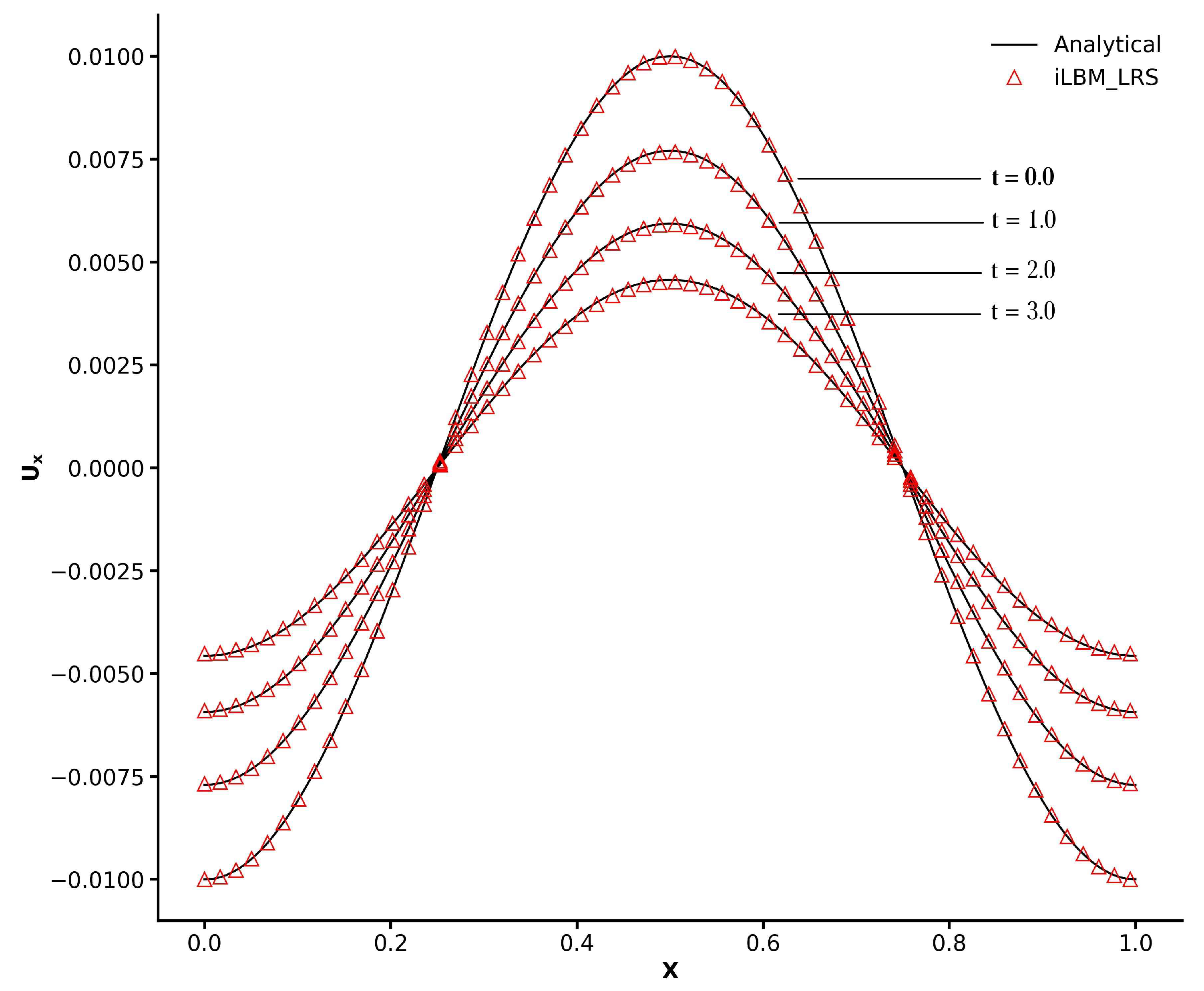
Figure 5 shows the x-direction velocity profiles along the location $y/W=0.75$ against the non-dimensional time t obtained using the FV-iLBM model in conjunction with the LR scheme. The non-dimensional time t is computed as $t=N_t\times \mathsf{\Delta }t$, where $N_t$ is the number of time steps. The time step $\mathsf{\Delta }t$ is taken as ${10}^{-4}$, whereas the relaxation parameter has been kept fixed at 0.01. The analytical solution at four different time instances—$t=0.0,1.0,2.0,$ and $3.0$—has been plotted. The iLBM model in conjunction with the LR scheme has produced excellent agreement with the analytical solution at different time instances. The excellent agreement between our numerical results and the analytical solution demonstrates that the FV-iLBM model with the LR scheme can accurately capture complex flow physics.

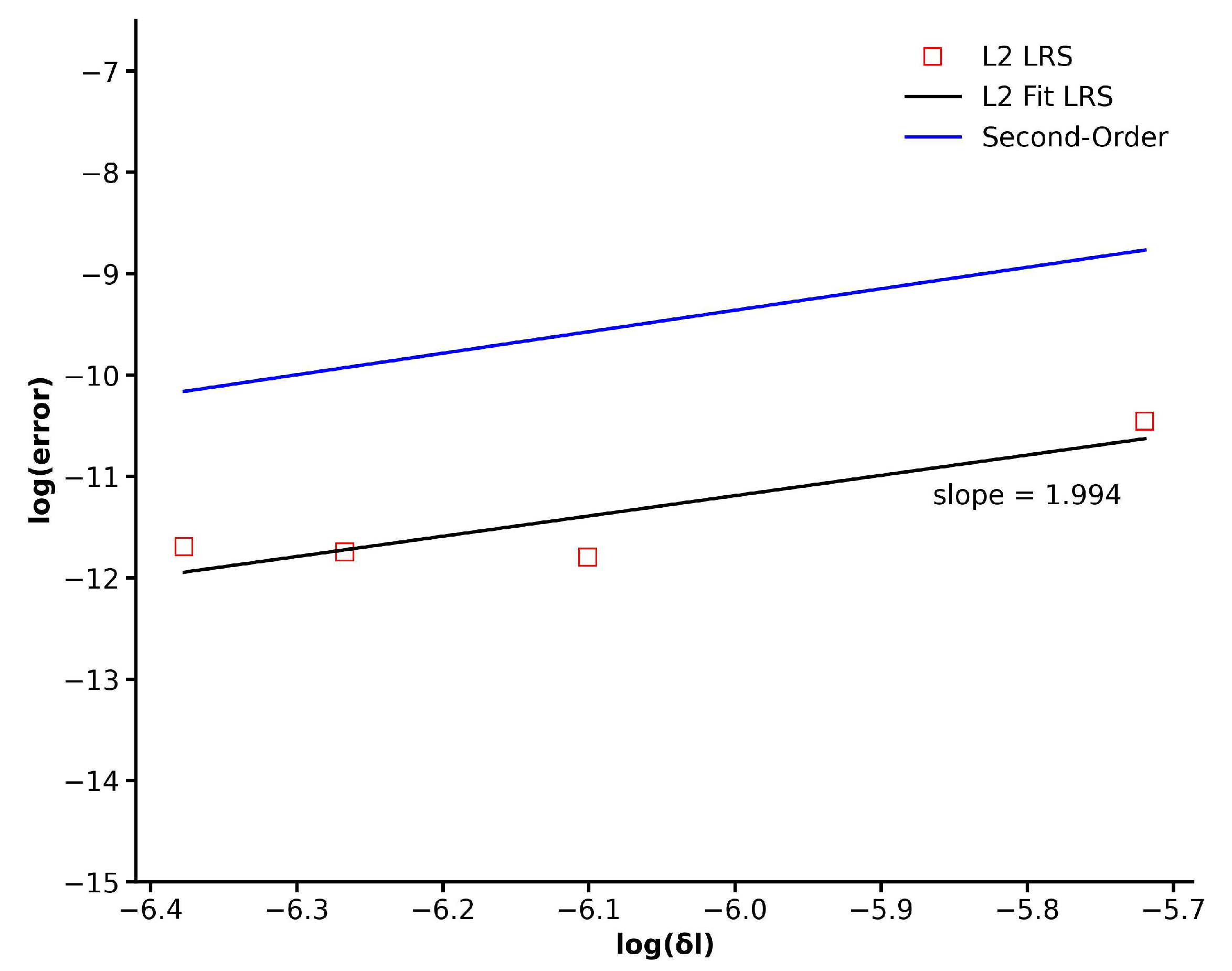
In order to perform error estimation to evaluate the order-of-accuracy, simulations have been performed using four different grids with increasing mesh refinement. Four grids with a total cell count of 37,986, 67,836, 139,792, and 253,942 cells have been used for this purpose. As the mesh is refined, the characteristic length $\delta l$, representing the smallest length of an edge in mesh, as well as the error obtained using $L1,L2$ and $L\infty$ norms should decrease, giving us an estimate of the order-of-accuracy. In Figure 6, the error assessment, determined through the $L2$ norm, is presented for the four grids mentioned above. It is evident that as the mesh undergoes refinement, the $L2$ error diminishes in a consistent second-order manner. This observation validates the second-order precision of the LR scheme integrated into the existing finite volume implementation of the iLBM model.

Table 1. The error norms (L1, L2, and L∞) with respect to mesh refinement for the Taylor–Green vortex flow simulation.

$\mathit{\delta }\mathit{l}$	L1 Error Norm	L2 Error Norm	L∞ Error Norm
$3.281\times {10}^{-3}$	$2.0413\times {10}^{-5}$	$2.8834\times {10}^{-5}$	$8.6470\times {10}^{-5}$
$2.241\times {10}^{-3}$	$5.9725\times {10}^{-6}$	$7.5234\times {10}^{-6}$	$2.3648\times {10}^{-5}$
$1.898\times {10}^{-3}$	$6.7683\times {10}^{-6}$	$7.9522\times {10}^{-6}$	$1.8634\times {10}^{-5}$
$1.70\times {10}^{-3}$	$7.0616\times {10}^{-6}$	$8.3448\times {10}^{-6}$	$2.0597\times {10}^{-5}$

quantifies the convergence behavior of the numerical scheme for the Taylor–Green vortex flow by reporting $L1,L2$ and $L\infty$ error norms across the progressively refined grids mentioned above. A systematic reduction in all error norms with decreasing characteristic length $\delta l$ indicates a consistent convergence of the solution. This trend validates the spatial accuracy of the method and its ability to resolve the flow field with increasing fidelity under grid refinement.

3.2. Decay of a Shear Wave

The attenuation of a shear wave with a wavelength equal to the domain size $(L=1)$ is discussed next. A square domain with both x- and y-direction boundaries set to periodic boundary conditions has been used for simulating the decay of a shear wave. The x- and y-direction velocities at the initial time instant $(t=0)$ have been taken as per those specified by Sofonea and Sekerka [55] and are given by

$$u\left(x,y,0\right)=Usin\left(2\pi y\right)$$

(50)

$$v\left(x,y,0\right)=0$$

(51)

where U has been set to $0.01$. At any time instant t, the analytical solution along the y-direction is given by

$$u\left(y,t\right)=U{e}^{-4\pi \nu t}sin\left(2\pi y\right)$$

(52)

The relaxation parameter has been taken as 0.01, while the time step $\mathsf{\Delta }t$ is taken as ${10}^{-4}$. As the solution marches in time, the initial shear wave at time instant $t=0$ decays, and the x-direction velocity profiles corresponding to different time instants obtained using the iLBM model in conjunction with the LR scheme and AB2 time integration method have been compared with the analytical solution in Figure 7. The results shown in Figure 7 have been obtained using an unstructured triangular mesh where a majority of the elements were equilateral triangles with a total cell count of 238,244 cells. As observed, the velocity profiles obtained using the iLBM model in conjunction with the LR scheme agree well with the analytical solution with minor disagreement for $t>8$.

In the finite volume framework, the discretization of the advection term in LBE induces certain numerical viscosity [15], which affects the accuracy of the scheme used to solve the advection term. Ideally, the apparent kinematic viscosity should be equal to the physical value of the viscosity. Sofonea and Sekerka [55] extracted the kinematic viscosity from the numerical results using

$$\nu ={\displaystyle \frac{1}{4{\pi }^{2}t}}log\left[{\displaystyle \frac{A\left(0\right)}{A\left(t\right)}}\right]$$

(53)

where the Fourier coefficient, $A\left(t\right)$, can be obtained as

$$A\left(t\right)={\int }_0^{L}u\left(y,t\right)sin\left(2\pi y\right)dy$$

(54)

In the above simulation, we have kept the relaxation parameter $\tau$ fixed at 0.01 and as per Equation (14), and the resultant kinematic viscosity value is $3.33\times {10}^{-3}$ in LBM units. Figure 8 shows the time evolution of kinematic viscosity. The kinematic viscosity obtained using the LR scheme is approximately $3.31\times {10}^{-3}$, which is within $1\%$ of the target value. This shows that very minimal non-physical numerical diffusion is present in the current numerical predictions obtained by the LR scheme and that it always maintains second-order accuracy.

3.3. Developing Flow in a 2D Channel

Developing flow in a 2D channel has been simulated using a rectangular domain $(L=5.0,W=1.0)$. Providing a uniform velocity at the inlet, the flow is allowed to develop in the channel, and the velocity profile obtained at the outlet is compared with the analytical solution. At the inlet, a uniform velocity profile using $U=0.1$ is provided and the pressure is linearly extrapolated from the interior domain, whereas at the outlet, the pressure is fixed $(P_{out}=1.0)$ and the velocity is linearly extrapolated from the interior domain. At the top and bottom walls, no-slip condition is applied using the NEE scheme [35] and the normal gradient of pressure is taken as zero.

A Reynolds number of 100 based on the inlet velocity and channel width has been simulated and time step taken as $\tau /10$. Figure 9a shows the outlet velocity profile (mesh with 120 elements in the y-direction and 500 elements in the x-direction with a total cell count of 120,000 cells) obtained using the FV-iLBM model in conjunction with the LR scheme, which accurately captures the velocity profile.

Figure 9b shows the distribution of pressure along the length of the channel at the centerline. In the entrance region of the pipe, there is an acceleration of flow, leading to a transition from a uniform velocity profile at the entrance to a fully developed profile by the end of this entrance region. Consequently, the pressure gradient magnitude is higher in the entrance region compared to that in the fully developed region. Once the flow is fully developed, the pressure gradient remains constant. A non-zero pressure gradient arises due to viscous forces, resulting in a pressure drop from the channel entrance to the fully developed region as pressure force is required to overcome the resistance produced by viscous forces.

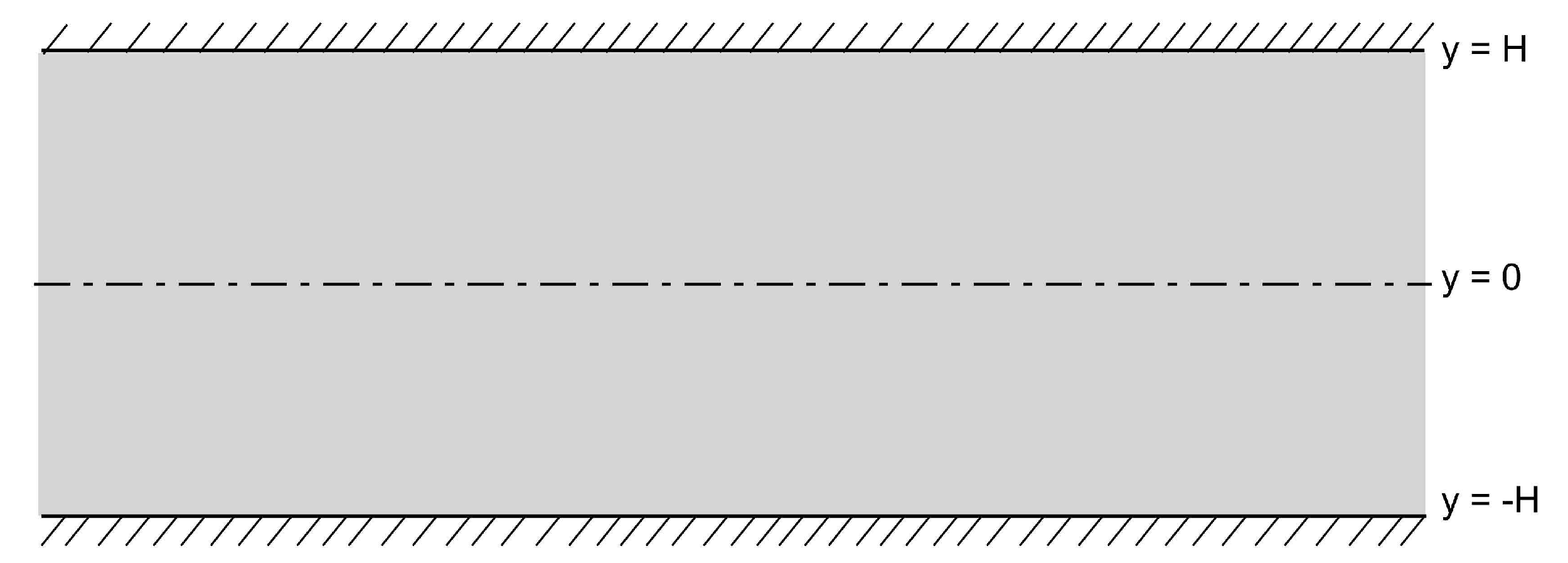
3.4. Womersley Flow

The capabilities of the FV-iLBM model to simulate the transient flow has been tested using the Womersley flow [56] in a 2D channel. NEE no-slip conditions are applied on the top and bottom walls of the channel. A time-dependent pressure difference $dP$ is applied on the inlet and the flow is driven by the fluctuation of pressure gradient $dP$ given by

$${\displaystyle \frac{\mathsf{\partial }P}{\mathsf{\partial }x}}=Re\left(A{e}^{i\omega t}\right)$$

(55)

where $A=dP/L_x$ and the analytical solution is given by [56]

$$u_x\left(y,t\right)=Re\left[{\displaystyle \frac{iA{e}^{i\omega t}}{\omega }}\left(1-{\displaystyle \frac{cos\left(\lambda \left(2y/L_y-1\right)\right)}{cos\lambda }}\right)\right]$$

(56)

where $\lambda =\sqrt{-i{\alpha }^2}$, $\omega$ is the frequency of the pressure pulse, and $\alpha$ is the Womersley number representing the relationship of transient inertial forces to viscous forces, given by

$$\alpha =L_y\sqrt{{\displaystyle \frac{\omega }{\nu }}}$$

(57)

The Womersley number ($\alpha$) considered here is $4.045$ and the pressure gradient $dP$ applied is $0.0032$ in LBM units. The Reynolds number simulated is 25. $L_x$ and $L_y$ represent the domain length in x- and y-direction, respectively, where $L_x=L_y=1.0$. An unstructured mesh with a total cell count of 85602 elements has been used to perform simulations. The maximum centerline velocity $u_{max}$ is calculated using the Hagen–Poiseuille equation. Once the Womersley number is chosen, the frequency of the pressure pulse is determined, which in turn determines the time period (T) as $2\pi /\omega$. 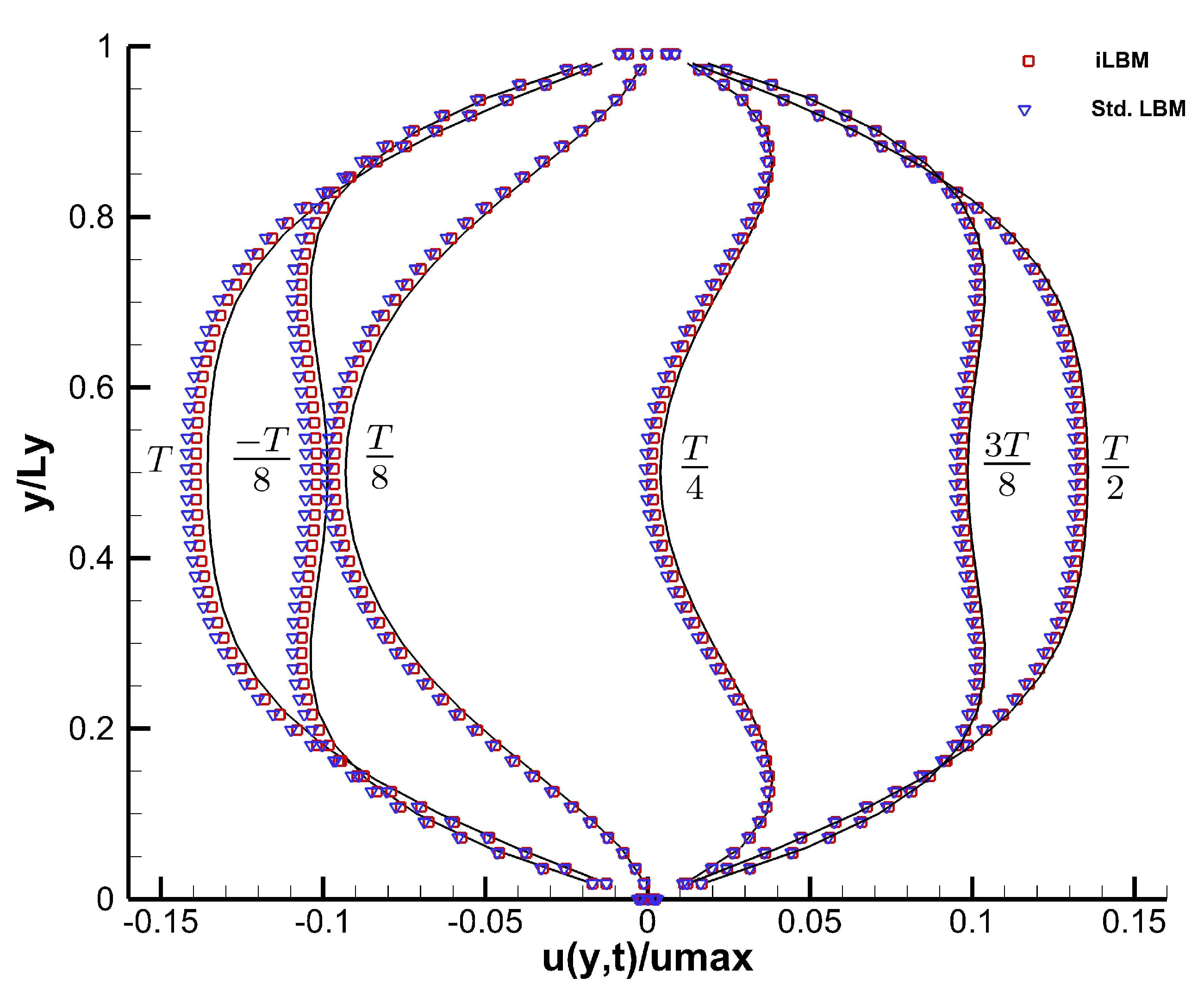Figure 10 shows the non-dimensional velocity profiles at different time periods (in factors of $1/8$) obtained using the iLBM model, in conjunction with the LR scheme, compared against the analytical solution of Equation (56). The velocity profiles have been extracted along the y-direction at $x=L_x/2$. The velocity profiles obtained using the standard LBM model have also been plotted to show a comparison with the iLBM model. As can be seen from Figure 10, velocity profiles obtained using the iLBM model are more accurate than those obtained using the standard LBM model.

Table 2. Comparison of analytical solution of $u_{max}$ at the center of the domain with that obtained using the FV-iLBM and standard LBM models. The % error in the parenthesis is calculated with respect to the analytical solution.

Time Period	Analytical	iLBM (% Error)	Std. LBM (% Error)
T/8	−0.0932108	−0.0966616 (3.70%)	−0.0989200 (6.12%)
T/4	0.0038521	0.0012198 (68.34%)	0.0007089 (81.59%)
3T/8	0.0986584	0.0966830 (2.0%)	0.0948343 (3.80%)
T/2	0.1356720	0.1334973 (1.60%)	0.1316358 (2.97%)

shows the comparison of the maximum centerline velocity ($u_{max}$) obtained using the iLBM and standard LBM models with the analytical centerline velocity, where the proficiency of the iLBM model over the standard LBM model is evident. The analytical value for centerline velocity at time period $T/4$ is very close to zero, where the numerical models will struggle to capture the velocity profiles. Thus, the centerline velocity values obtained using the iLBM and standard LBM models deviate from the expected results [17].

To further evaluate the performance of the iLBM model, a quantitative comparison was conducted against the standard LBM model (both models implemented in the finite volume framework) for the Womersley flow case. As summarized in

Table 3. Comparison of memory and runtime performance of the FV-iLBM model with the standard LBM model. The L2 error is calculated with respect to the analytical solution of the Womersley flow.

Metric	Standard LBM	iLBM	Improvement
Memory per cell (Bytes)	∼96	∼104	∼8.3% more
Runtime per iteration (s)	∼0.2207	∼0.1872	∼15.2% faster
L2 Error	0.00419	0.00262	∼38.9% accurate

, for a serial implementation, the iLBM model incurs a modest increase in memory usage per cell (∼104 bytes vs. ∼96 bytes) due to the inclusion of pressure terms. However, it achieves a significant improvement in both computational efficiency and accuracy, with a ∼15.2% reduction in runtime per iteration and a ∼38.9% lower L2 error. These results demonstrate that the FV-iLBM model offers a favorable trade-off between memory footprint and overall simulation performance, highlighting its potential for accurate and efficient incompressible flow simulations.

The proficiency of the iLBM model to limit the compressibility error while simulating pulsating flows is a significant finding of this study. Pulsating flows play a pivotal role in a wide array of fluid dynamics scenarios with applications ranging from cardiovascular health assessment to thermal energy engineering, electronic engineering, machinery manufacturing, chemical engineering, etc. Reciprocating compressors, pulse combustion chamber, microdiffusers, micropumps, and microchannels all feature pulsating flows. In electronic engineering, the rate of heat transfer is enhanced using pulsating flows. The iLBM model can be effectively used to simulate flows across these applications and explore the flow physics involved.

3.5. Lid-Driven Flow in a 2D Square Cavity

The steady state solution of a lid-driven flow in a 2D square cavity $(L=W=1)$ at different Reynolds numbers has been studied to assess the capabilities of the FV-iLBM solver. The Reynolds number, in this case, is based on the width of the cavity as $Re=UL/\nu$, where L is the cavity width and U is the velocity of the top plate. Four different Reynolds numbers have been simulated: 100, 400, 1000, and 3200. The wall velocity boundary condition given by Equation (39) has been applied to all the four walls of the cavity with a velocity of the top wall U set to 0.1. For the remaining three walls, the no-slip boundary condition has been imposed for velocity and the normal gradient of pressure has been taken as zero. The time step has been taken as $\tau /10$. The NSE results of Ghia et al. [57] have been considered as the benchmark solution here. The results obtained using the FV-iLBM model in conjunction with the LR scheme and AB2 time integration method are presented here.

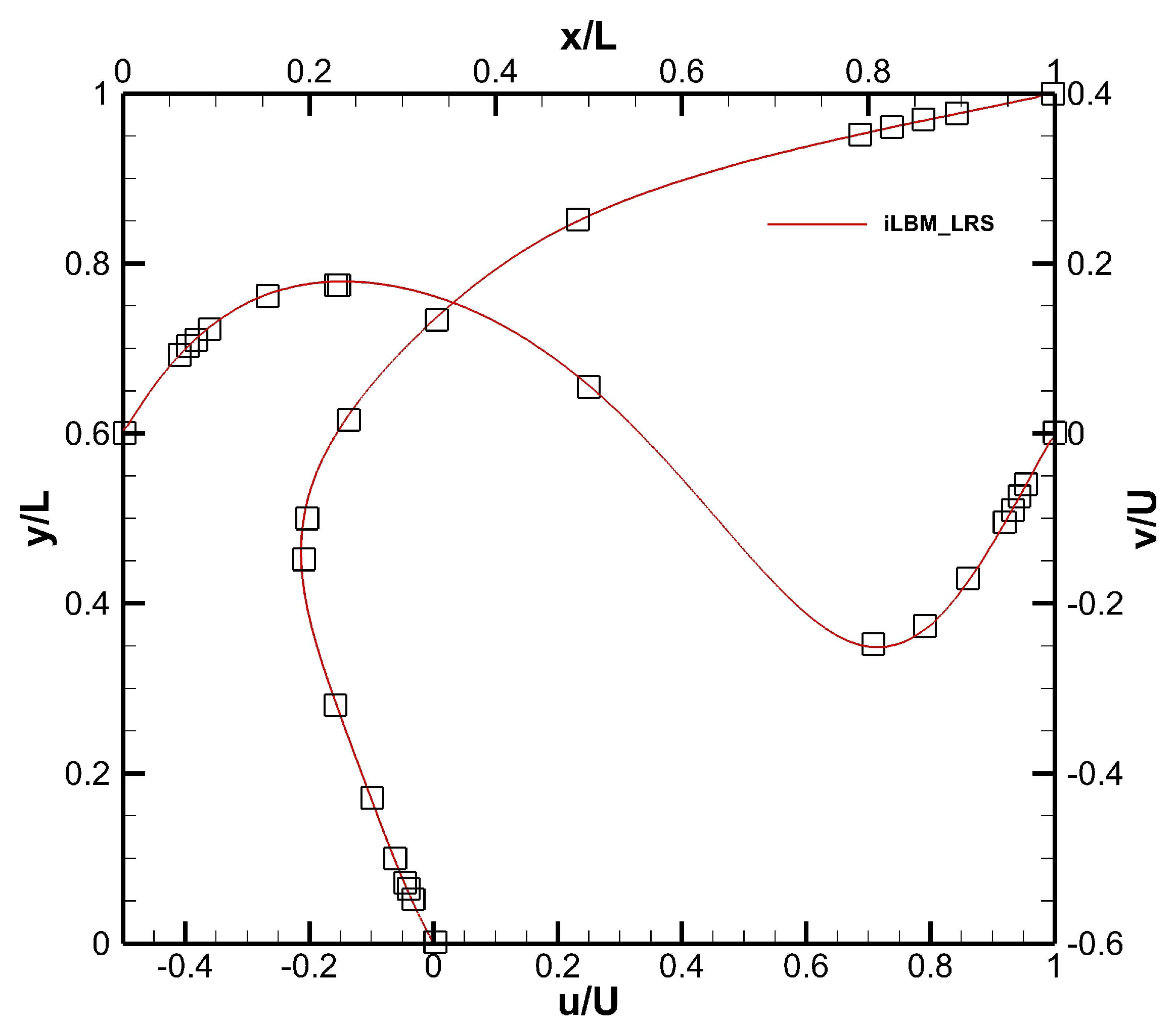
To simulate lid-driven flow for $Re=100$, an unstructured grid with 200 triangular cells on each wall and a total cell count of 105,692 cells has been used. Figure 11 shows the normalized axial and radial velocity profiles for $Re=100$. As can be observed from the figure, the FV-iLBM predictions agree well with the benchmark solution [57].

Table 4. X- and y-coordinates of the centers of primary, bottom right, and bottom left vortices for lid-driven flow with $Re=100,400$ and 1000 obtained using the FV-iLBM model.

Re	Study	Primary	Bottom Right	Bottom Left
	Ghia et al. [57]	(0.6172, 0.7344)	(0.9453, 0.0625)	(0.0313, 0.0391)
100	Patil et al. [15]	(0.6161, 0.7296)	(0.9451, 0.0574)	(0.0345, 0.0324)
	Present	(0.6149, 0.7390)	(0.9436, 0.0606)	(0.0345, 0.0342)
	Ghia et al. [57]	(0.5547, 0.6055)	(0.8906, 0.1250)	(0.0508, 0.0469)
400	Patil et al. [15]	(0.5506, 0.5972)	(0.8862, 0.1258)	(0.0526, 0.0471)
	Wang et al. [31]	(0.5543, 0.6061)	(0.8859, 0.1225)	(0.0507, 0.0471)
	Present	(0.5568, 0.6097)	(0.8862, 0.1236)	(0.0485, 0.0463)
	Ghia et al. [57]	(0.5313, 0.5625)	(0.8594, 0.1094)	(0.0859, 0.0781)
1000	Patil et al. [15]	(0.5259, 0.5777)	(0.8778, 0.1261)	(0.0904, 0.0989)
	Wang et al. [31]	(0.5310, 0.5665)	(0.8644, 0.1130)	(0.0828, 0.0774)
	Present	(0.5321, 0.5706)	(0.8640, 0.1160)	(0.0828, 0.0757)

lists the x- and y-coordinates of the centers of primary vortex, bottom right vortex, and bottom left vortex obtained for $Re=100$. The results obtained using the FV-iLBM approach are compared with the benchmark solution and those obtained by Patil et al. [15]. As observed, the FV-iLBM approach accurately captures the location of all the vortices.

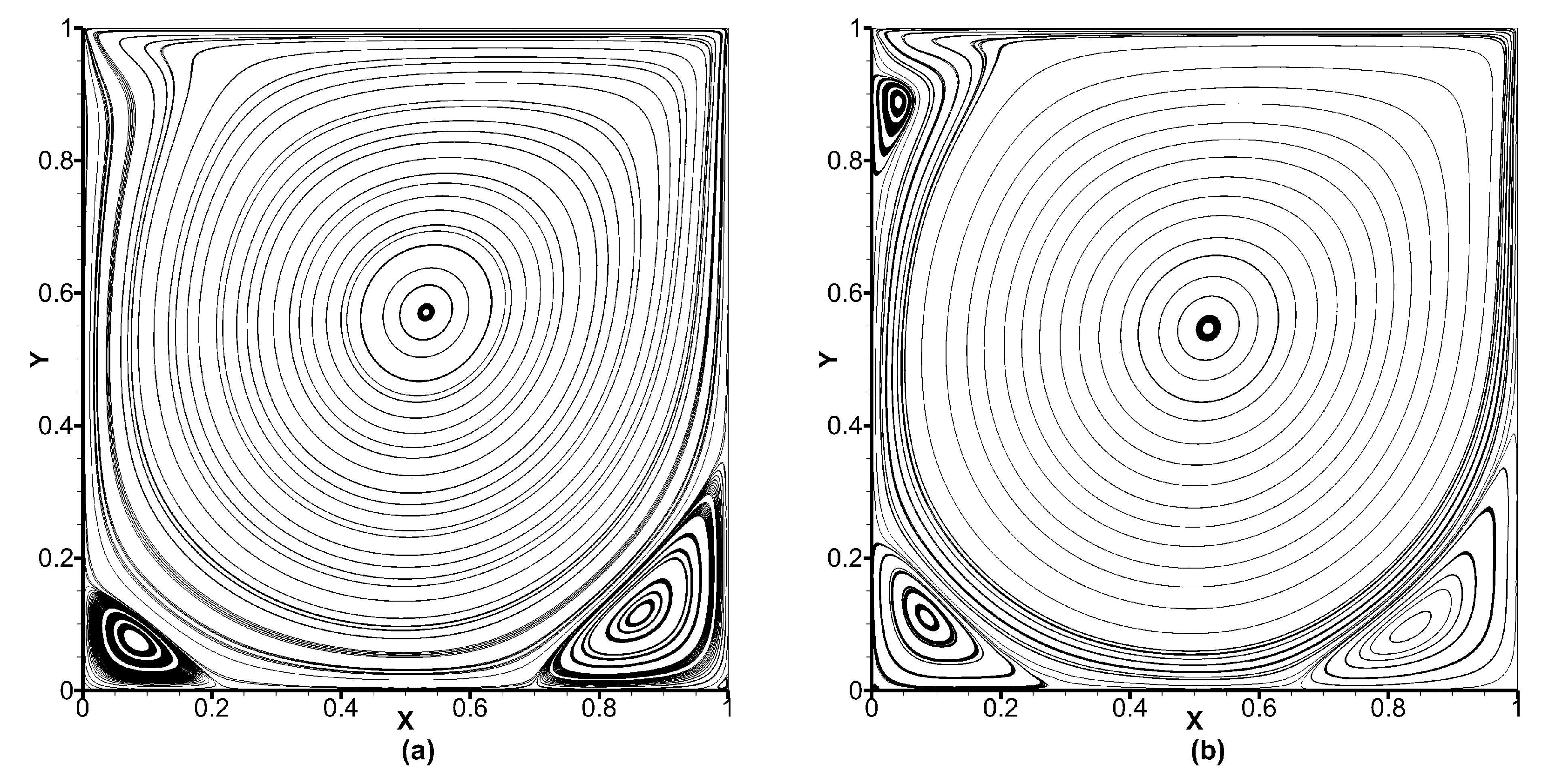
As the Reynolds number increases, the numerical predictions for the lid-driven flow depend on how well the boundary layer is resolved. Therefore, for simulating lid-driven flow with $Re=400,1000,$ and 3200, an unstructured grid with 250 triangular cells on each wall and a total cell count of 164,756 cells has been used. Figure 12 shows the streamlines obtained for the lid-driven flow with $Re=1000$ and 3200, and as observed, important flow features such as corner vortices including the top left corner vortex for $Re=3200$ has been captured by the FV-iLBM model, implying that the boundary layer has been adequately resolved.

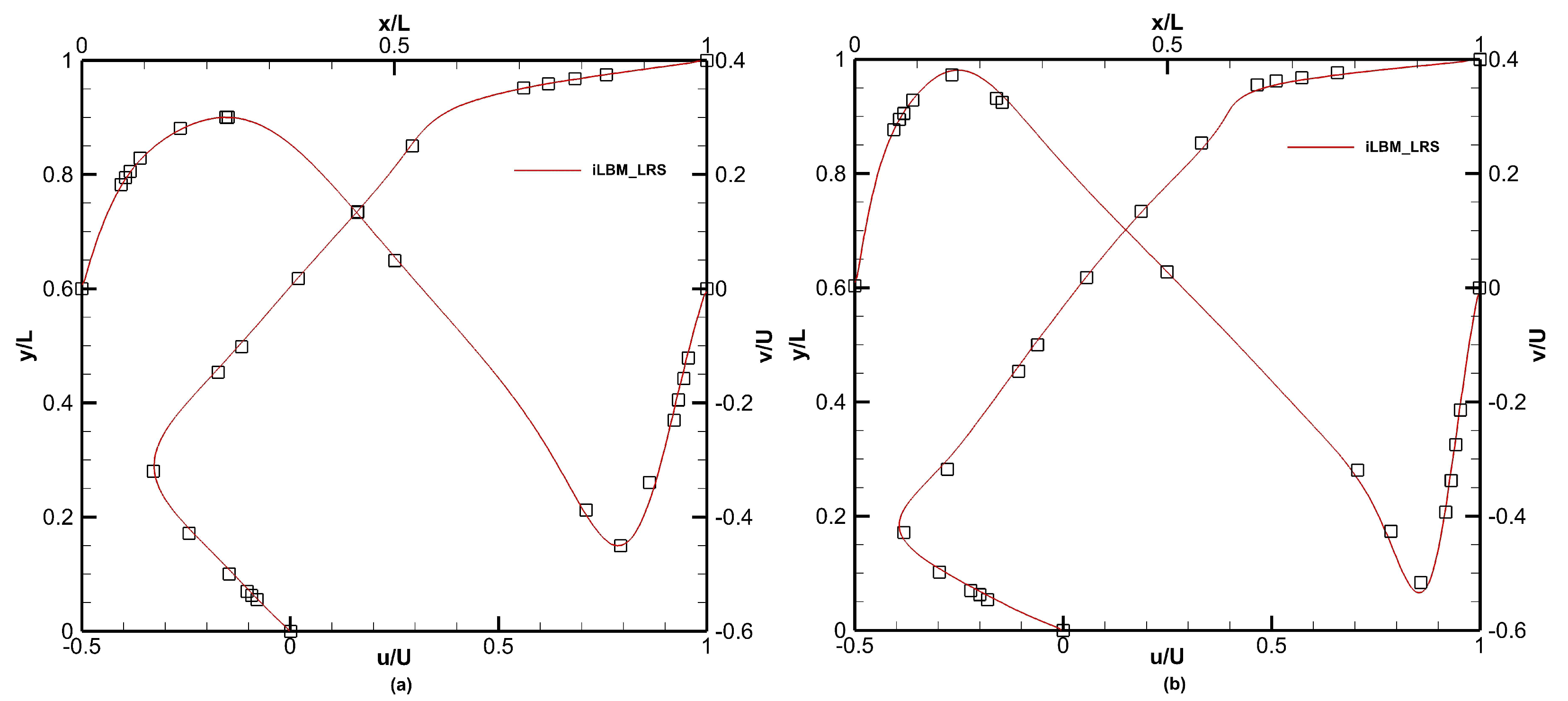
Figure 13 shows the normalized axial and radial velocity profiles for lid-driven flow with $Re=400$ and $Re=1000$, respectively. The FV-iLBM model in conjunction with the LR scheme captures the velocity profiles accurately. Table 4 lists the x- and y-coordinates of primary, bottom right, and bottom left vortices for lid-driven flow with $Re=400$ and $Re=1000$. As the Reynolds number increases, the locations of the vortices produced by the FV-iLBM model agree well with the benchmark solution. Comparing the vortex locations produced by the FV-iLBM model with those obtained by Patil et al. [15] and Wang et al. [31], FV-iLBM predictions are competitive with both of these studies for $Re=400$. For $Re=1000$, the FV-iLBM predictions are better than those obtained by Patil et al. [15] and are competitive with those obtained by Wang et al. [31].

For $Re=1000$, we have also compared the width and height of the corner vortices obtained using the FV-iLBM model with benchmark [57] and those obtained by Patil et al. [15] and Wang et al. [31]. As shown in

Table 5. Width and height of the corner vortices for lid-driven flow with $Re=1000$ obtained using the FV-iLBM model.

	Bottom Left		Bottom Right
	Width	Height	Width	Height
Ghia et al. [57]	0.2188	0.1680	0.3034	0.3536
Patil et al. [15]	0.2167	0.2005	0.2888	0.3431
Wang et al. [31]	0.2151	0.1641	0.2970	0.3530
Present	0.2113	0.1613	0.3011	0.3623

, the size of the bottom left vortex obtained using the FV-iLBM model agrees adequately with the benchmark solution and is competitive with those obtained by Patil et al. [15] and Wang et al. [31]. For the bottom right vortex, the FV-iLBM model produces superior results than both of these studies and agrees well with the benchmark solution.

Figure 14 shows the normalized axial and radial velocity profiles obtained for $Re=3200$ using the FV-iLBM model in conjunction with the LR model. The FV-iLBM predictions are compared with those obtained by Patil et al. [15] to make a qualitative comparison. The FV-iLBM predictions agree well with the benchmark solution and are superior to those obtained by Patil et al. [15]. As pointed out by Wang et al. [31], the numerical predictions obtained by Patil et al. [15] suffer from non-physical numerical diffusion, resulting in disagreement between their numerical predictions and the benchmark solution.

Table 6. X- and y-coordinates of the centers of primary, bottom right, bottom left, and top left vortices for lid-driven flow with $Re=3200$ obtained using the FV-iLBM model.

	Ghia et al. [57]	Patil et al. [15]	Present
Primary	(0.5165, 0.5469)	(0.5189, 0.5441)	(0.5190, 0.5417)
Bottom Right	(0.8125, 0.0859)	(0.8619, 0.0971)	(0.8335, 0.0932)
Bottom Left	(0.0859, 0.1094)	(0.0993, 0.0963)	(0.0859, 0.1087)
Top Left	(0.0547, 0.8984)	(0.0316, 0.8689)	(0.0416, 0.8875)

lists the x- and y-coordinates of the centers of primary, bottom right, bottom left, and top left vortices, whereas

Table 7. Width and height of the corner vortices for lid-driven flow with $Re=3200$ obtained using the FV-iLBM model.

	Bottom Left		Bottom Right		Top Left
	Width	Height	Width	Height	Width	Height
Ghia et al. [57]	0.2844	0.2305	0.3406	0.4102	0.0859	0.2057
Patil et al. [15]	0.3146	0.2443	0.3018	0.3925	0.0494	0.1819
Wang et al. [31]	0.2816	0.2356	0.3358	0.3839	0.0877	0.1938
Present	0.2840	0.2234	0.3397	0.4049	0.0662	0.1667

details the width and height of the corner vortices obtained for the lid-driven flow with $Re=3200$. The locations of corner vortices obtained using the FV-iLBM model in conjunction with the LR scheme agree well with the benchmark solution and are superior to those obtained by Patil et al. [15]. Barring the size of the top left vortex, the width and height of the bottom left and bottom right vortices produced by the FV-iLBM model are very close to the benchmark solution, are superior to those obtained by Patil et al. [15], and are close to those obtained by Wang et al. [31].

3.6. Flow over NACA0012 Airfoil

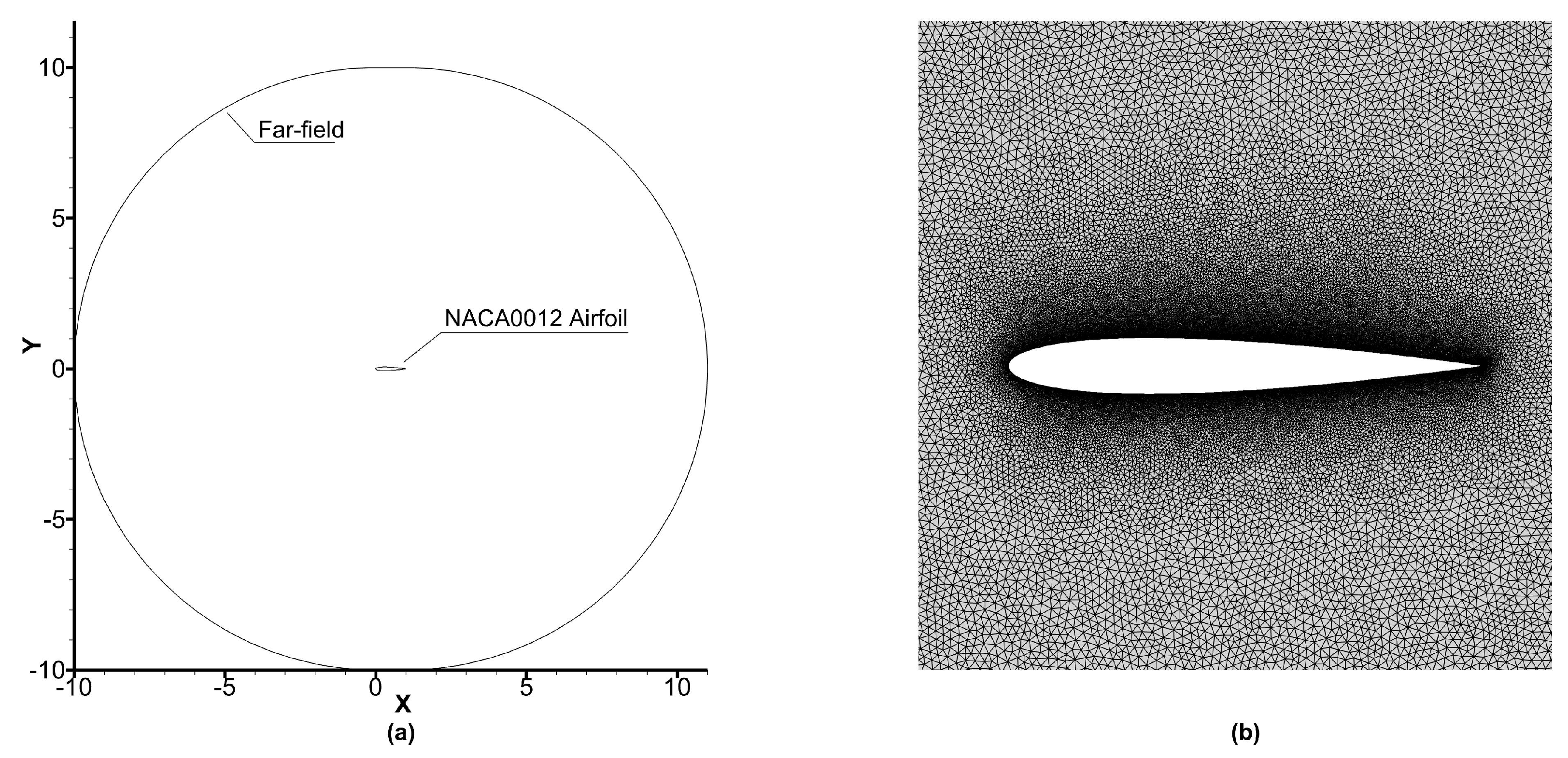
External flow over the NACA0012 airfoil with a Reynolds number of 1000 has been simulated using the FV-iLBM model. Reynolds number, in this case, is defined as $Re=U_{\infty }L/\nu$. Here, $U_{\infty }=0.1$ is the free-stream velocity, $L=1.0$ is the chord length, and $\nu$ is the kinematic viscosity. Figure 15a shows the schematic of the domain used for simulating flow over the NACA0012 airfoil. The far-field boundary is located at 10L in all directions from the stagnation point, which is large enough to eliminate the influence of far-field boundary on the flow.

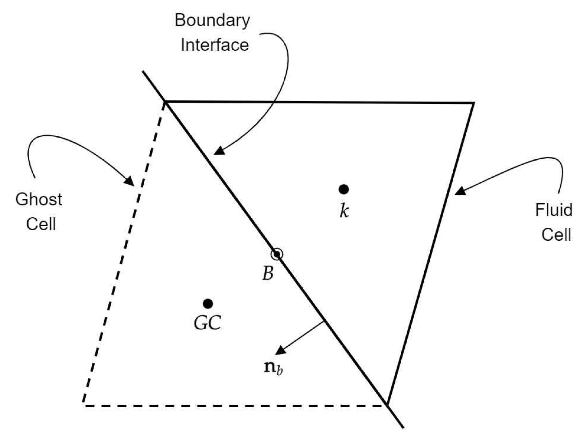
The far-field boundary condition is applied using ghost cells in conjunction with Equations (40), (59), and (60) as

$$f_{\alpha ,GC}=f_{\alpha }^{eq}\left(P_{\infty },{\mathbf{u}}_x,{\mathbf{u}}_y\right)+f_{\alpha ,k}-f_{\alpha ,k}^{eq}$$

(58)

where $P_{\infty }=1.0$ is the free-stream pressure in LBM units. On the airfoil surface, the no-slip boundary condition has been imposed for velocity and the normal gradient of pressure has been taken as zero. The time step has been taken as $\tau /10$.

We have studied four different angles of attack: $7^{\circ }$, $8^{\circ }$, $9^{\circ }$, and ${11}^{\circ }$. The velocity components corresponding to different angles of attack are set as

$$u_x=U_{\infty }cos\left({\displaystyle \frac{\theta \pi }{180}}\right)$$

(59)

$$u_y=U_{\infty }sin\left({\displaystyle \frac{\theta \pi }{180}}\right)$$

(60)

where $\theta$ represents the angle of attack in degrees.

We have used three different unstructured grids with cell counts of 38,710 (grid 1), 75,868 (grid 2), and 120,520 cells (grid 3) having 198, 398, and 798 cells on the airfoil surface, respectively. The grid is refined by refining the cell count surrounding the airfoil as shown in Figure 15b.

To understand the effect of grid refinement on numerical predictions, we have simulated the flow over the NACA0012 airfoil at an angle of attack of $8^{\circ }$ and plotted the distribution of pressure coefficient $\left(c_p\right)$ on the airfoil surface. The NSE solution of Kurtulus [58] has been used as the benchmark solution in the present study. The distribution of $c_p$ on the airfoil surface is computed as

$$c_p={\displaystyle \frac{\left(P-P_{\infty }\right)}{\frac{1}{2}{\rho }_{\infty }{U}_{\infty }^2}}$$

(61)

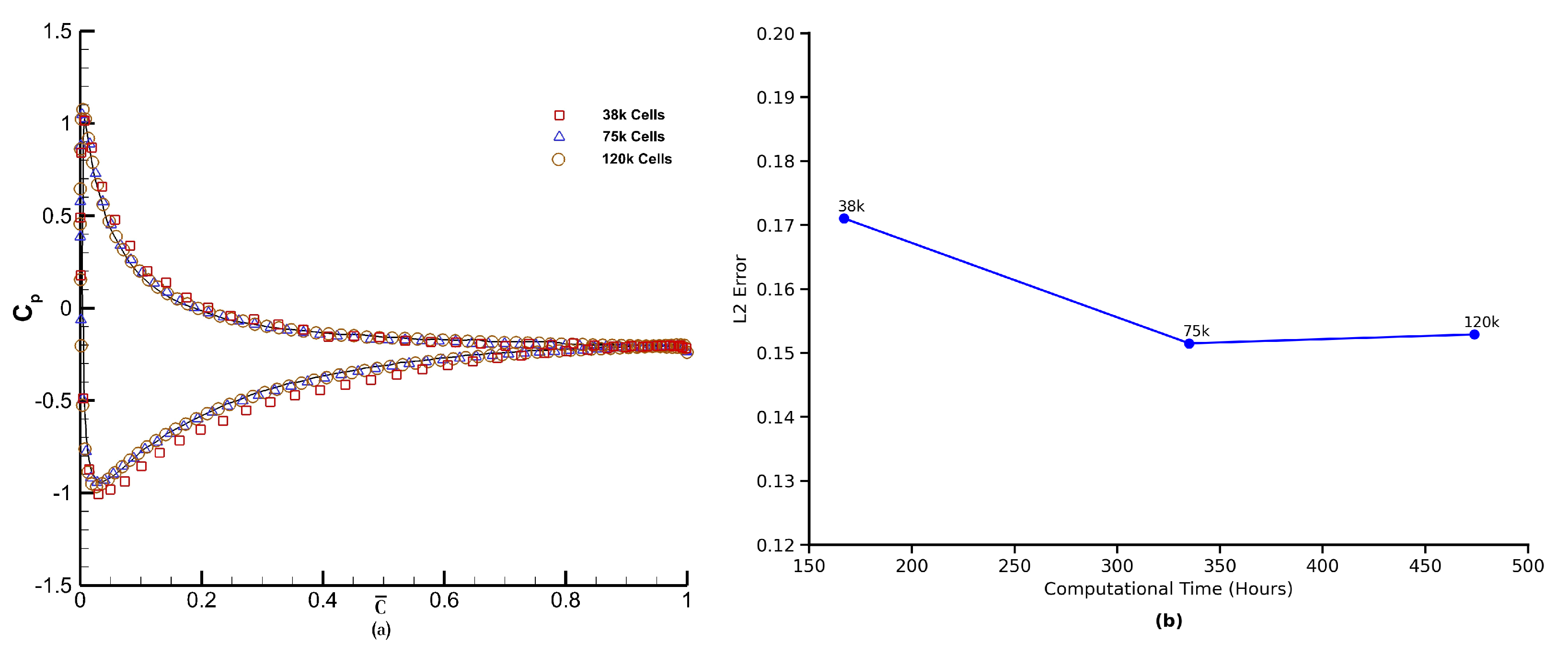
Figure 16a shows the distribution of mean pressure coefficient for angle of attack $8^{\circ }$ obtained using the FV-iLBM model using the three grids mentioned above. The $c_p$ profile obtained using grid 1 captures the distribution adequately on the bottom surface; however, it also shows disagreement with the benchmark solution on the top surface. Grid 2 and grid 3 accurately capture the $c_p$ distribution on both the top and bottom surfaces of the airfoil. Based on this analysis, we have used grid 2 for the remaining analysis. Furthermore, to evaluate the trade-off between accuracy and computational efficiency, we examined the L2 error as a function of total runtime for three successively refined grids (38 k, 75 k, and 120 k cells). As shown in Figure 16b, the error decreases significantly when increasing resolution from 38 k to 75 k cells, reducing from 0.171 to 0.151. However, further refinement to 120 k cells yields minimal improvement (L2 error = 0.1529) while increasing runtime from 335 to 473.8 h—an increase of ∼41%. This trend illustrates a classic diminishing return with respect to grid refinement and motivates the choice of the 75 k cell grid for the bulk of our simulations as the optimal compromise between accuracy and computational cost.

The Karman vortex street theory, studying the flow around bluff bodies, describes the occurrence of periodic vortex shedding, which in the case of a flow over an airfoil depends on the angle of attack. Figure 17 depicts the instantaneous streamlines for flow over the NACA0012 airfoil for $Re=1000$ and angles of attack, $\theta =7^{\circ },8^{\circ },9^{\circ }$ and ${11}^{\circ }$. The initiation of unsteady vortex shedding has been observed at angle of attack $8^{\circ }$, and as the angle of attack is increased further, an enlargement of flow instabilities at the rear of the airfoil has been observed. These observations are in line with those pointed out in the literature [58,59].

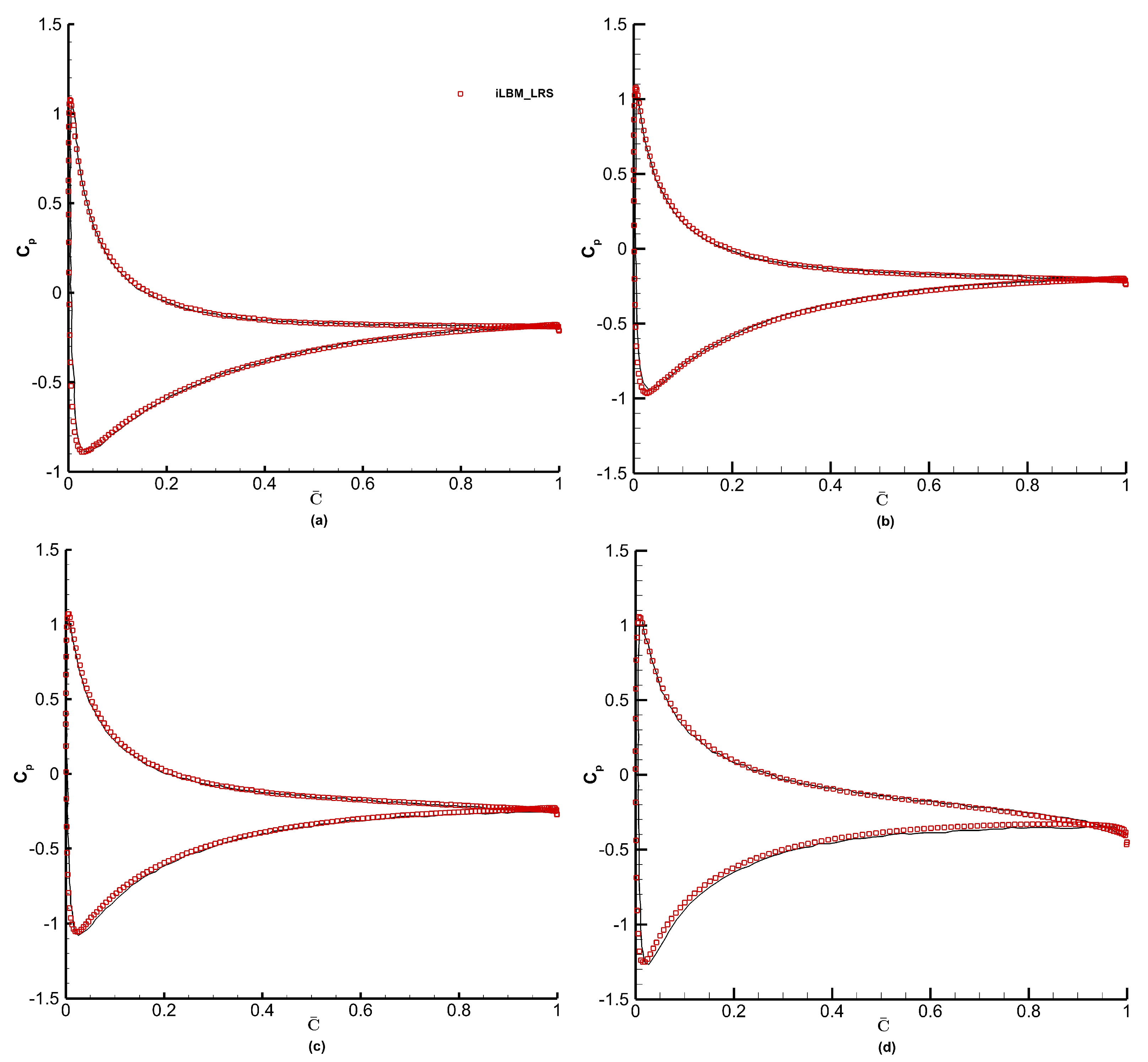
The distribution of mean pressure coefficient along the non-dimensional chord $\overline{C}$ for angles of attack $\theta =7^{\circ },8^{\circ },9^{\circ }$ and ${11}^{\circ }$ is shown in Figure 18. The $c_p$ profiles obtained using the FV-iLBM model are compared with those available in ref. [58]. The $c_p$ distribution over both lower and upper airfoil surfaces obtained using the FV-iLBM model agrees well with those from the literature. As stated above, as $\theta$ increases, the flow instabilities at the rear of the airfoil grow in size along the trailing edge, where a very minor disagreement between FV-iLBM predictions and the benchmark [58] has been observed for $\theta ={11}^{\circ }$.

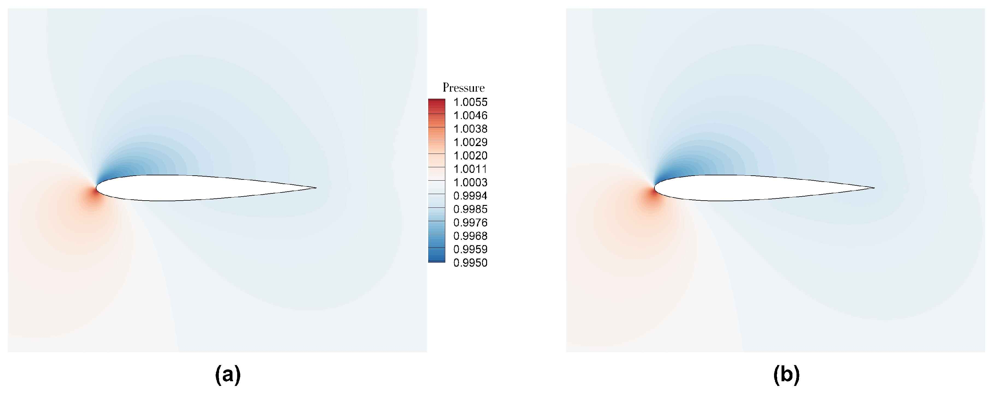
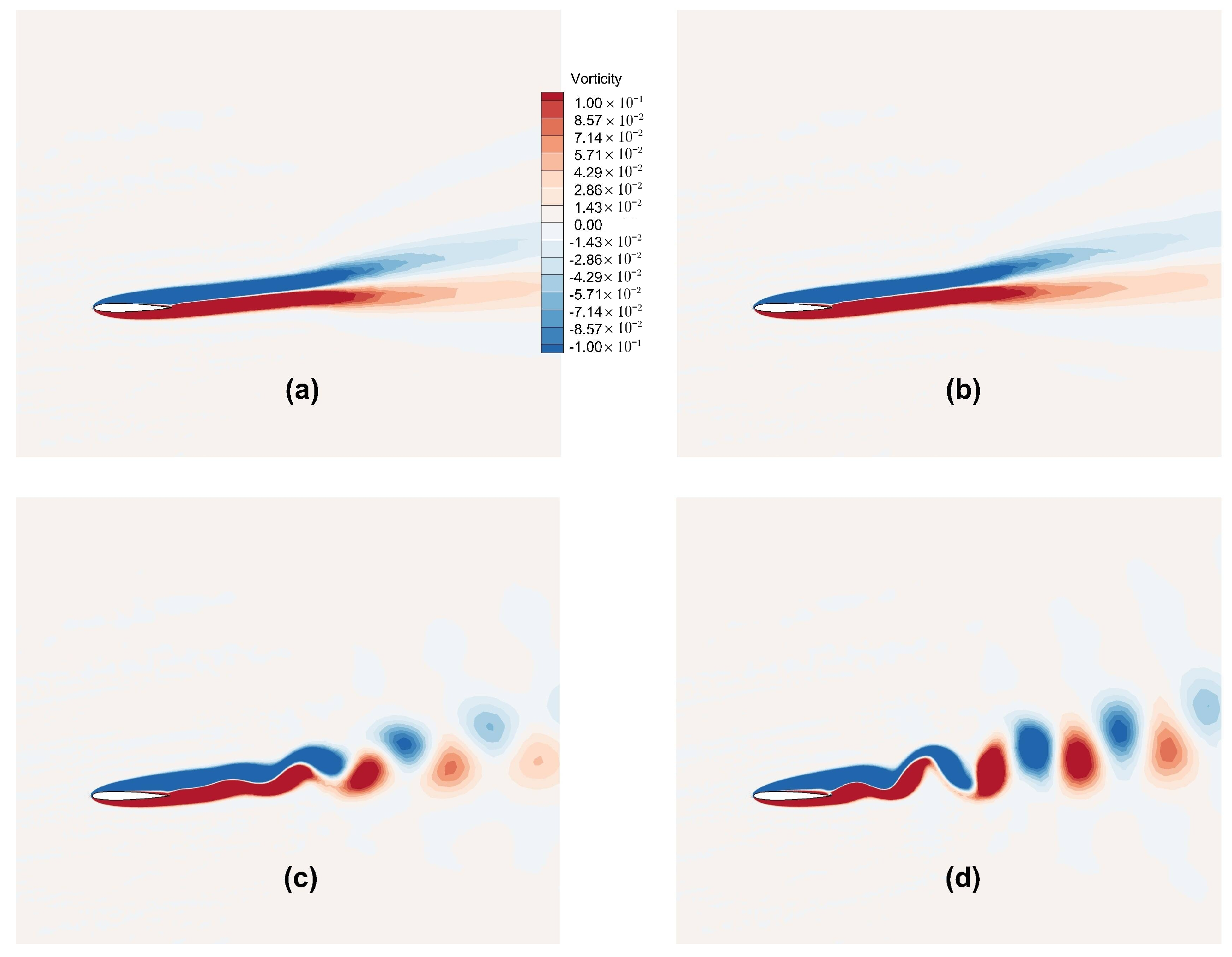
Figure 19 shows the instantaneous pressure field. Figure 20 shows the instantaneous vorticity contours. As the angle of attack is increased, we observe the onset of lift generation and an observation of onset of unsteady vortex shedding at $8^{\circ }$. Vortex shedding becomes apparent at $9^{\circ }$, giving rise to the formation of two counter-rotating vortices. As the angle of attack increases further, there is an augmentation in the strength of vortices, which is in line with the observation in Figure 17.

Overall, a good agreement is observed between the FV-iLBM predictions and those from the ref. [58] with the FV-iLBM model producing consistent and encouraging results. As the FV-iLBM predictions transition from the symmetric flow at lower angles of attack to the onset of lift generation, flow separation, and increased pressure drag at higher angles, these findings highlight the airfoil’s sensitivity to the changes in angle of attack and the capability of the present FV-iLBM solver to accurately capture the flow physics of the unsteady aerodynamic applications.

3.7. Validation of FV-iLBM Solver for Non-Newtonian Fluid Flow

The FV-iLBM model has been validated for non-Newtonian fluid flow by simulating the flow through a straight as well as a stenosed channel and comparing the results with those provided by Janela et al. [50]. The Carreau model [41] has been used to simulate the non-Newtonian blood viscosity.

As explained in Section 2.7, the Carreau model [41] simulates the effective viscosity using Equation (32). In the Carreau model, the parameter $\lambda$ governs the transition region where the viscosity drop occurs and has the unit of time (s). The Carreau model is most sensitive to ${\mu }_0$ and $\lambda$, which can have substantial impact on numerical predictions. They are essentially derived from extrapolated data due to technical challenges associated with measuring viscosity at low shear rates [50]. The FV-iLBM model has been validated by modeling the non-Newtonian flow through a 2D straight channel with different values of $\lambda$. The schematic of the 2D straight channel is shown in Figure 21.

The selected geometry and flow conditions are suitable for simulating blood flow in an arteriole. The flow conditions [50] are as follows:

$$\begin{array}{c}\hfill \rho =1{\mathrm{g}/\mathrm{cm}}^3{U}_{max}=2.2\mathrm{cm}/\mathrm{s}H=0.02\mathrm{cm}\\ \hfill {\mu }_0=0.56Poise{\mu }_{\infty }=0.0345Poise\end{array}$$

(62)

Using Equation (33), the Reynolds number is found to be 0.157. Considering the physiological range [50], two different $\lambda$ values, namely 0.01 and 0.1 s, have been simulated using the FV-iLBM model in conjunction with the LR scheme.

The flow domain shown in Figure 21 has been normalized to a rectangle of dimension [−3, 3] × [−1, 1] and the flow conditions mentioned in Equation (62) are scaled from physical units to LB units using Equation (35), Equation (36), and Equation (37). Following Janela et al. [50], the scaling parameter, $\beta$, from Equation (35) has been taken as $0.05$. After scaling into the LB units, we have the following flow conditions:

$$\begin{array}{c}\hfill \overline{\rho }=1.0{\overline{U}}_{max}=0.0022\overline{H}=1.0\\ \hfill {\overline{\mu }}_0=0.0280{\overline{\mu }}_{\infty }=0.001725\end{array}$$

(63)

The power-law index (n) in the Carreau model (Equation (32)) has been taken as 0.3568 and $\lambda$ has been carefully scaled in LB units using Equation (37). The iLBM model [17] is a pressure-based LBM scheme derived from a constant density ($\overline{\rho }=1.0$), and density plays no further part in the iLBM’s formulation.

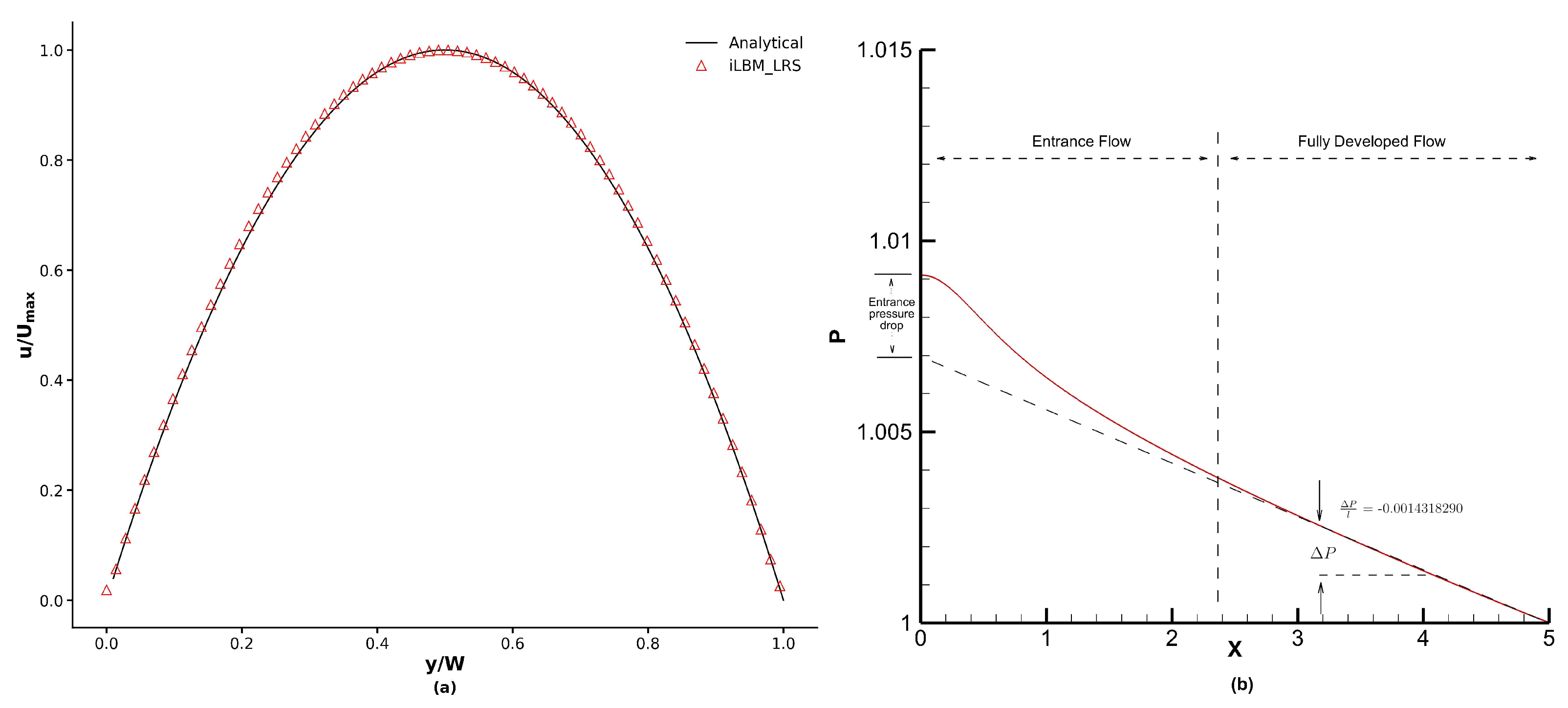
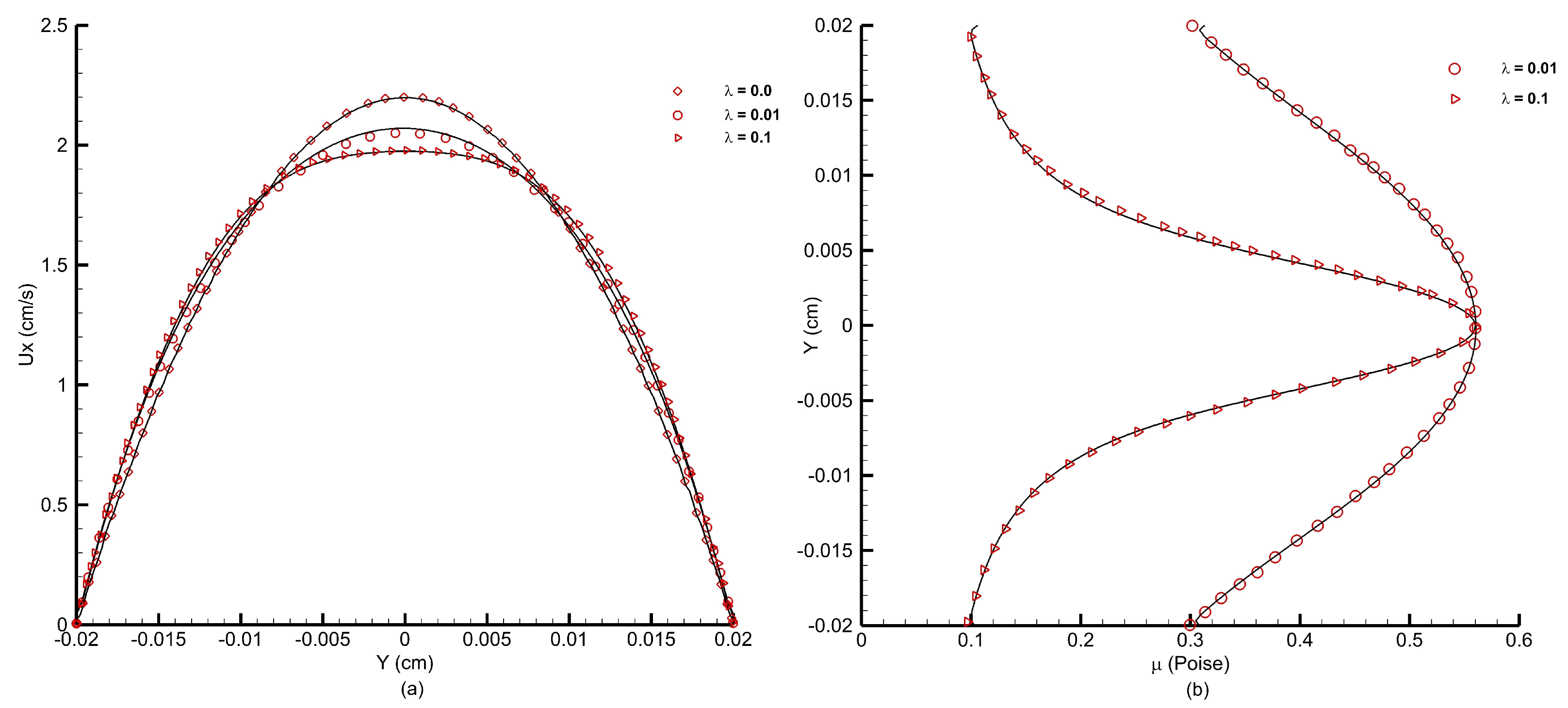
A parabolic velocity profile with a maximum velocity $U_{max}$ is enforced at inlet, whereas at the outlet, the pressure is fixed ($\overline{P}=1.0$) and the velocity is linearly extrapolated from the interior domain. No-slip condition is applied at the top and bottom walls using the NEE scheme [35] and the normal gradient of pressure is taken as zero. Figure 22a shows the velocity profiles obtained using the FV-iLBM model for different $\lambda$ values. A Newtonian case with $\lambda =0.0$ s has also been simulated for comparison. As the $\lambda$ value increases, the velocity profile flattens at the core of the channel due to a larger value of viscosity at low shear rates, and the FV-iLBM model has accurately captured this trend.

Figure 22b shows the viscosity profiles for $\lambda =0.01,$ and $0.1$ s. As the $\lambda$ value increases, the viscosity also increases along the core of the channel changing from almost a parabolic profile at a lower $\lambda$ value to a more refined profile at a higher $\lambda$ value, which is in line with the flattening of the velocity profile at the core of the channel observed in Figure 22a. As observed from Figure 22b, the FV-iLBM model accurately captures the effect of different $\lambda$ values on viscosity.

The FV-iLBM model has also been validated for modeling non-Newtonian flow through a stenosed channel. For this purpose, a 2D channel with a longitudinal span of $[-L,L]$ and a stenosis centered at $x=0$ as shown in Figure 23 has been considered.

Figure 23 shows the schematic of the 2D channel used to simulate the flow of blood through arterial stenosis. The stenosis or constriction is obtained using the following equation [50]:

$${\displaystyle \frac{H\left(x\right)}{H_0}}=1-\delta e^{\varphi \left(x/H_0\right)}$$

(64)

where $H\left(x\right)$ is the height of the channel, $\delta$ is the degree of stenosis, and $\varphi$ is the length of the stenosis. To maintain a slowly varying profile of stenosis, a sufficiently small $\varphi$ should be chosen. Different degrees of stenosis ($\delta$), in a circular cross-section, can be calculated as follows [60]:

$$\%stenosis=100\left(1-{\left(1-\delta \right)}^2\right)$$

(65)

A flow obstruction of 50%, as shown in Figure 23, has been obtained using the following parameters [50]:

$$\delta =0.3\varphi =0.8$$

In the present study, following Janela et al. [50] and Cho and Kinsey [61], the following parameters are used for the Carreau model:

$$\lambda =0.15\mathrm{s}n=0.3568{\mu }_0=0.56Poise{\mu }_{\infty }=0.0345Poise$$

The flow is driven by a pressure gradient. Following Janela et al. [50], this gradient matches that of flow in a straight channel with $\lambda =0.15$ s and $n=0.3568$. A no-slip condition is applied at the top and bottom walls using the NEE scheme [35], with a zero normal gradient of pressure. At the outlet, the pressure is fixed at $\overline{P}=1.0$, and the velocity is linearly extrapolated from the interior domain. With $H_0$ = 0.02 cm, L = 0.1 cm, and $\rho =1$ ${\mathrm{g}/\mathrm{cm}}^3$, the selected geometry and flow conditions are consistent with blood flow in an arteriole or small artery.

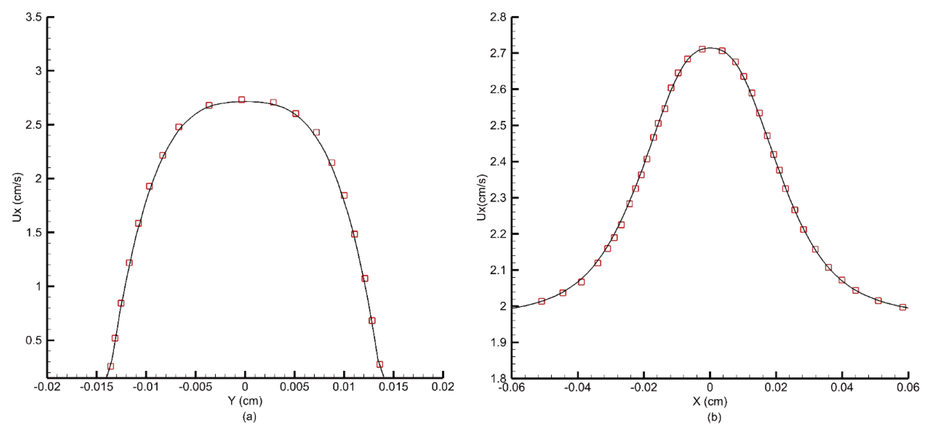
Figure 24 shows the velocity profiles obtained at the throat of the stenosis and at the centerline along the length of the channel. Figure 25 shows the viscosity profile at the throat of the channel. For the Carreau model, when $\lambda >0.1$ s, the viscosity shows a prominent peak along the centerline due to low shear stress [50]. The FV-iLBM model accurately captures this effect and predicts both velocity and viscosity profiles accurately.

3.8. Blood Flow Through an Artery Afflicted with Multiple Stenoses

Based on the results above, the finite volume iLBM approach can be used to simulate cardiovascular fluid dynamics effectively. The effects of different cardiovascular flow conditions on the well-being of arterial health can be quantified using parameters such as time-averaged wall pressure (TAWP), time-averaged wall shear stress (TAWSS), and oscillatory shear index (OSI). These indices are computed by time-averaged wall shear stress over one cardiac cycle. TAWSS, which is a measure of wall shear stress for one cardiac cycle, is computed as

$$TAWSS={\displaystyle \frac{1}{T}}{\int }_0^T\left|{\sigma }_w\right|dt$$

(66)

OSI—which is used to identify regions where the flow deviates most from its average direction and wall shear stress fluctuates the most—is computed as

$$OSI={\displaystyle \frac{1}{2}}\left[1-{\displaystyle \frac{\left|{\int }_0^T{\sigma }_{w}dt\right|}{{\int }_0^T\left|{\sigma }_w\right|dt}}\right]$$

(67)

Time-averaged wall pressure (TAWP) is computed as

$${\overline{P}}_w={\displaystyle \frac{1}{T}}{\int }_0^T{P}_{w}dt$$

(68)

Using these indices, regions of low and oscillatory wall shear stress can be identified, which can be used to understand the factors that contribute to the progression of cardiovascular diseases such as atherosclerosis.

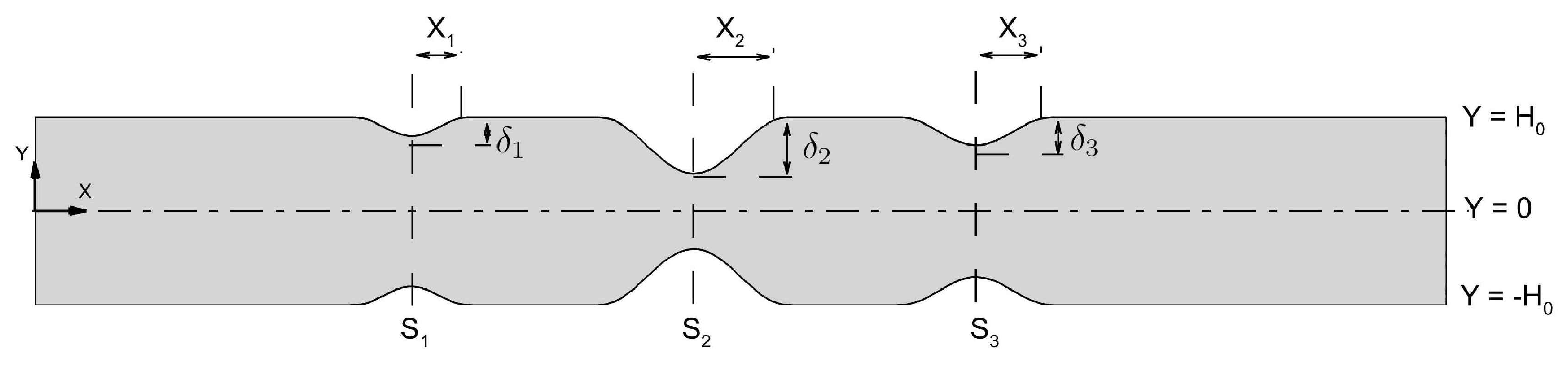
The coronary artery, a vital vessel supplying oxygen-rich blood to the myocardium, has a complex geometry often affected by multiple stenoses [62]. Simplifying its structure while preserving key characteristics is essential for studying arterial hemodynamics. Figure 26 illustrates the schematic of an artery with triple stenoses, each of varying severity. In the figure, $S_i$ denotes the stenosis location, i is the stenosis index, X represents the half-length, $\delta$ the severity, and $H_0$ the channel half-width.

The triple stenoses shown in Figure 26 has been obtained using Equation (69) as

$$H\left(x\right)=\left\{\begin{array}{cccc}{H}_0-{\displaystyle \frac{{\delta }_i}{2}}\left(1+cos\left({\displaystyle \frac{\pi \left(x-S_i\right)}{x_i}}\right)\right)& & & \left(S_i-X_i\right)<x<\left(S_i+X_i\right)\\ & & & i=1,2,3\\ \\ H_0& & & otherwise\end{array}\right.$$

(69)

Table 8. Severity of stenosis for different $\delta$ values.

$\mathit{\delta }$	X	Severity of Stenosis (%)	Designation
0.2	0.6	36	S
0.3	0.8	51	M
0.6	1.0	84	L

shows different degrees of stenosis for corresponding $\delta$ values that have been considered in the present study. The third column in Table 8, titled designation, facilitates reference for terminology in the discussion. Here, S, M, and L denote ‘small’, ‘medium’, and ‘large’ stenosis severity, respectively. The configuration shown in Figure 26 is termed ‘S-M-L’ configuration.

The human coronary artery diameter typically ranges from 3 to 5 mm. In this study, for a 2D planar domain (Figure 26), an artery height ($2H_0$) of 5 mm is considered. The model parameters representing blood flow in human arteries have been considered as per Abbasian et al. [63]. They are as follows:

$$\begin{array}{c}\hfill \lambda =3.313\mathrm{s}n=0.3568\\ \hfill {\mu }_0=0.56Poise{\mu }_{\infty }=0.0345Poise\end{array}$$

The problem is scaled to LB units by setting the scaling parameter to $\beta =0.03$. In Figure 26, the locations of stenoses are as follows:

$$S_1=4.0S_2=7.0S_3=10.0$$

Considering the pulsatile nature of blood flow through the arteries, a pulsatile velocity has been set at the inlet of the artery using

$$u_{in}\left(t\right)={\displaystyle \frac{Q\left(t\right)}{A}}$$

(70)

where A is the cross-sectional area of the inlet surface and $Q\left(t\right)$ is the pulsatile flow rate. Considering a 2D planar domain, the cross-sectional area is calculated considering unit width. Referring to Figure 26, if $2H_0$ is the artery height and W is the width of the artery, then the cross-sectional area is calculated as $A=2H_0\times 1.0$.

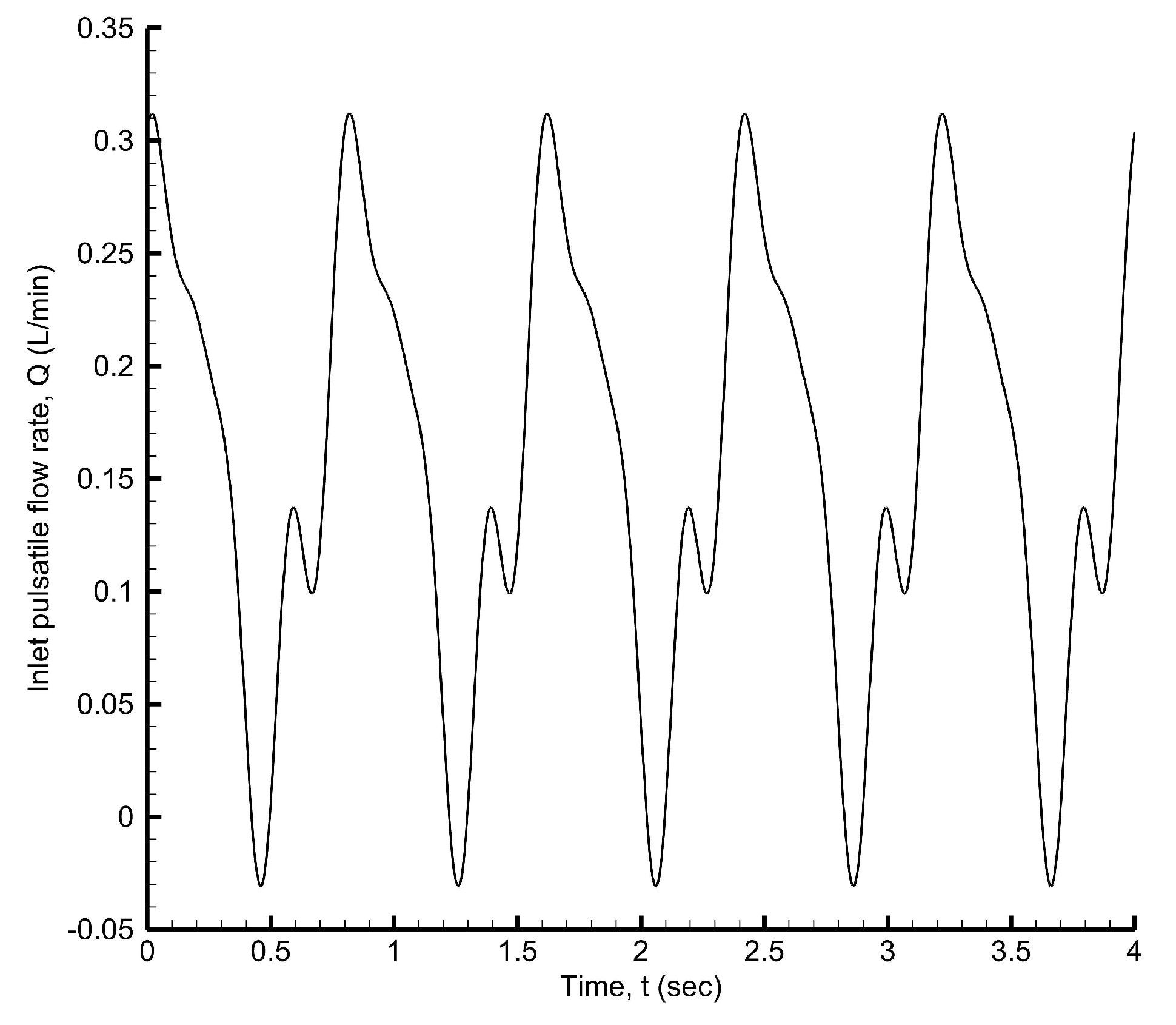
The inlet pulsatile velocity is derived from the pulsatile flow rate waveform [64] shown in Figure 27, which is expressed using the Fourier series as

$$Q\left(t\right)=\overline{Q}+\sum _{n=1}^4{A}_n^{Q}cos\left(n\omega t\right)+B_n^{Q}sin\left(n\omega t\right)$$

(71)

The coefficients $A_n^Q$ and $B_n^Q$ are obtained using the MATLAB 2021b curve fitting tool. The coefficients are obtained using the [65] curve fitting tool and are listed in

Table 9. Fourier series coefficients for pulsatile flow rate (Q).

n	${\mathit{A}}_{\mathit{n}}^{\mathit{Q}}$	${\mathit{B}}_{\mathit{n}}^{\mathit{Q}}$
1	0.1011	0.07513
2	−0.00352	−0.00835
3	0.0316	0.03158
4	0.01809	−0.01486

.

The time-averaged volumetric flow rate obtained using the MATLAB curve fitting tool is $\overline{Q}=0.158$ L/min. The pulsatile inlet velocity is scaled to LB units using Equation (36). In Equation (71), the angular velocity $\omega$ relates to the cardiac cycle as $T=2\pi /\omega$. The waveform [64] shown in Figure 27 has a time period of $T=0.8$ s, corresponding to an average pulse rate of 75 beats/min. Given the coronary artery diameter, the Womersley number is $\alpha =3.88$ and the Reynolds number is $Re=80$. Three cardiac cycles are simulated with a time step of $0.03{\mu }_0$, as shown in Figure 27.

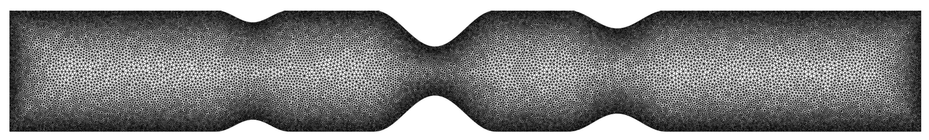
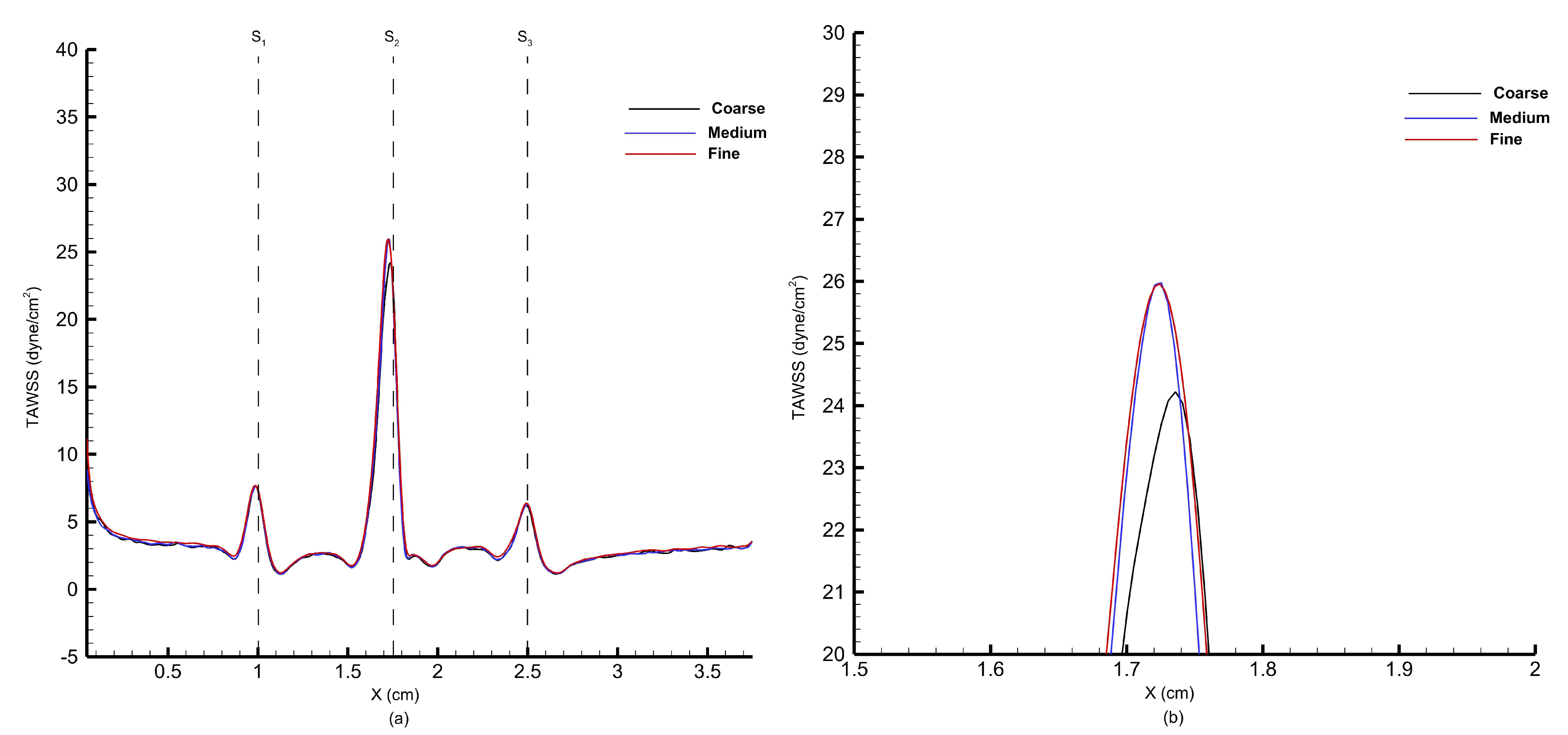
Figure 28 illustrates the unstructured triangular mesh used for the S-L-M configuration, with a highly refined grid near the artery walls to accurately capture flow physics and a progressively coarser mesh toward the core to optimize cell count. A grid independence study was conducted using three meshes: grid 1 (coarse) with 519 wall cells and 41,772 elements, grid 2 (medium) with 802 wall cells and 72,600 elements, and grid 3 (fine) with 1209 wall cells and 99,892 elements. As shown in Figure 29, the wall shear stress profiles from grid 2 and grid 3 closely match, and therefore, grid 2 has been selected for the blood flow analysis through multiple stenoses.

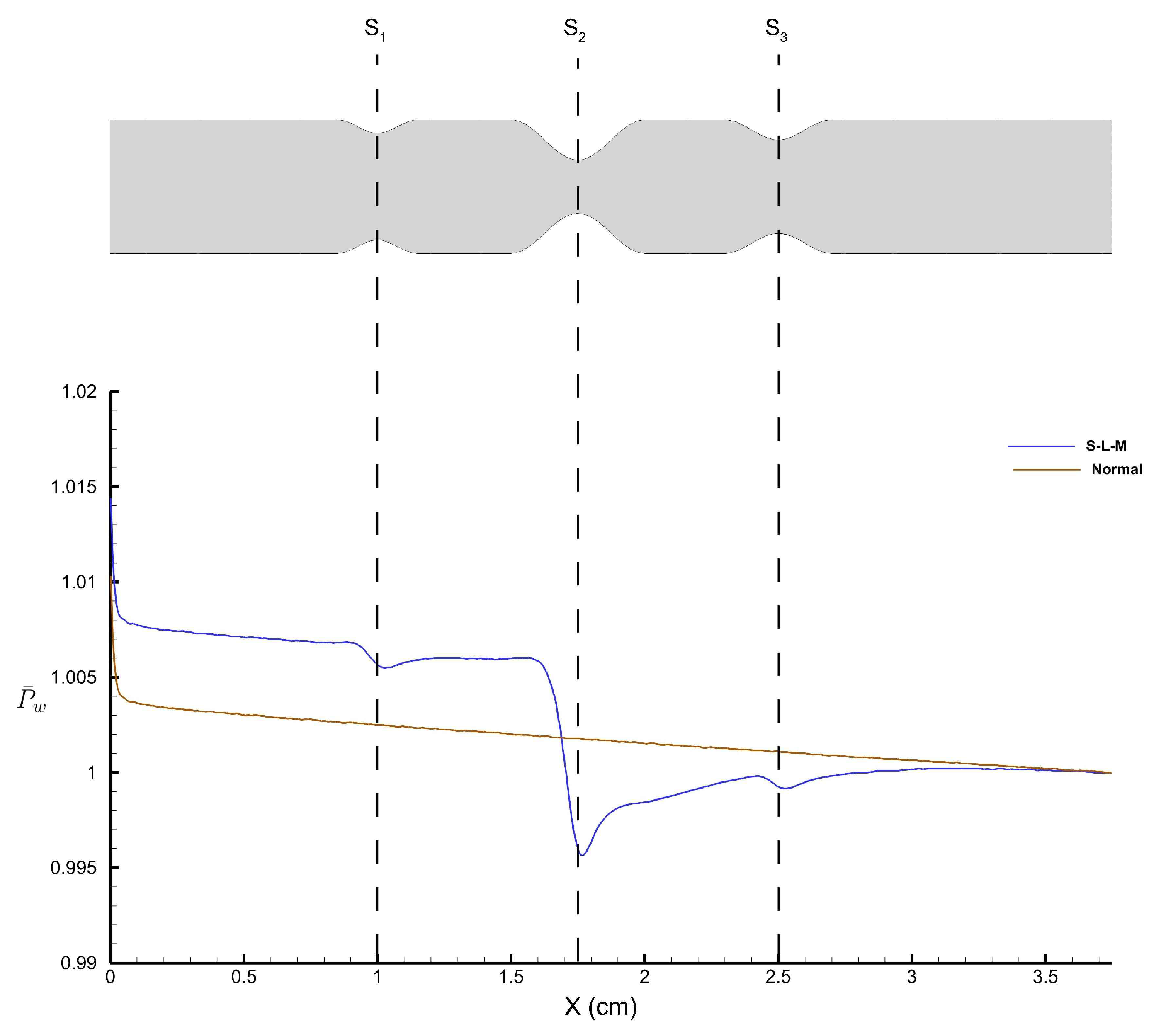
The pressure along the arterial wall plays a critical role in the development of arterial diseases. Figure 30 shows the time-averaged wall pressure along the top wall of the stenosed artery obtained using the FV-iLBM model. $S-L-M$ refers to the wall pressure obtained along the top wall of the stenosed artery with the S-L-M stenosis configuration, whereas ‘$normal$’ refers to the wall pressure obtained for the normal artery without any stenosis.

As the flow encounters the small stenosis, we observe a drop in pressure and attempts to recover post the stenosis. However, the flow encounters the large stenosis and we observe the largest pressure drop, after which we observe pressure recovery. A final dip in pressure distribution is observed after the the medium stenosis; however, it does not affect the wall pressure substantially. On the other hand, a linearly decreasing pressure profile is observed for the normal artery, which is the normal tendency of the fluid pressure due to friction along the length of the artery wall.

As fluid flow approaches the narrowing (stenosis) in the artery, there is a sudden drop in pressure with the lowest wall pressure corresponding to the highest average velocity of fluid flow. The cross-sectional area for flow decreases as it approaches the stenosis, reaching its minimum at the narrowest point (throat), then increases again as it moves toward the exit of the stenosis. According to the principle of continuity for incompressible fluids, the average velocity of flow is inversely proportional to the cross-sectional area. Therefore, the maximum average velocity at the stenosis throat corresponds to the minimum pressure at that point. Following a sharp pressure drop at the stenosis, there is a partial recovery in wall pressure downstream due to the conversion of kinetic energy into pressure energy in the diverging section of the stenosis. However, the pressure does not return to its original value due to irreversible losses caused by viscous effects.

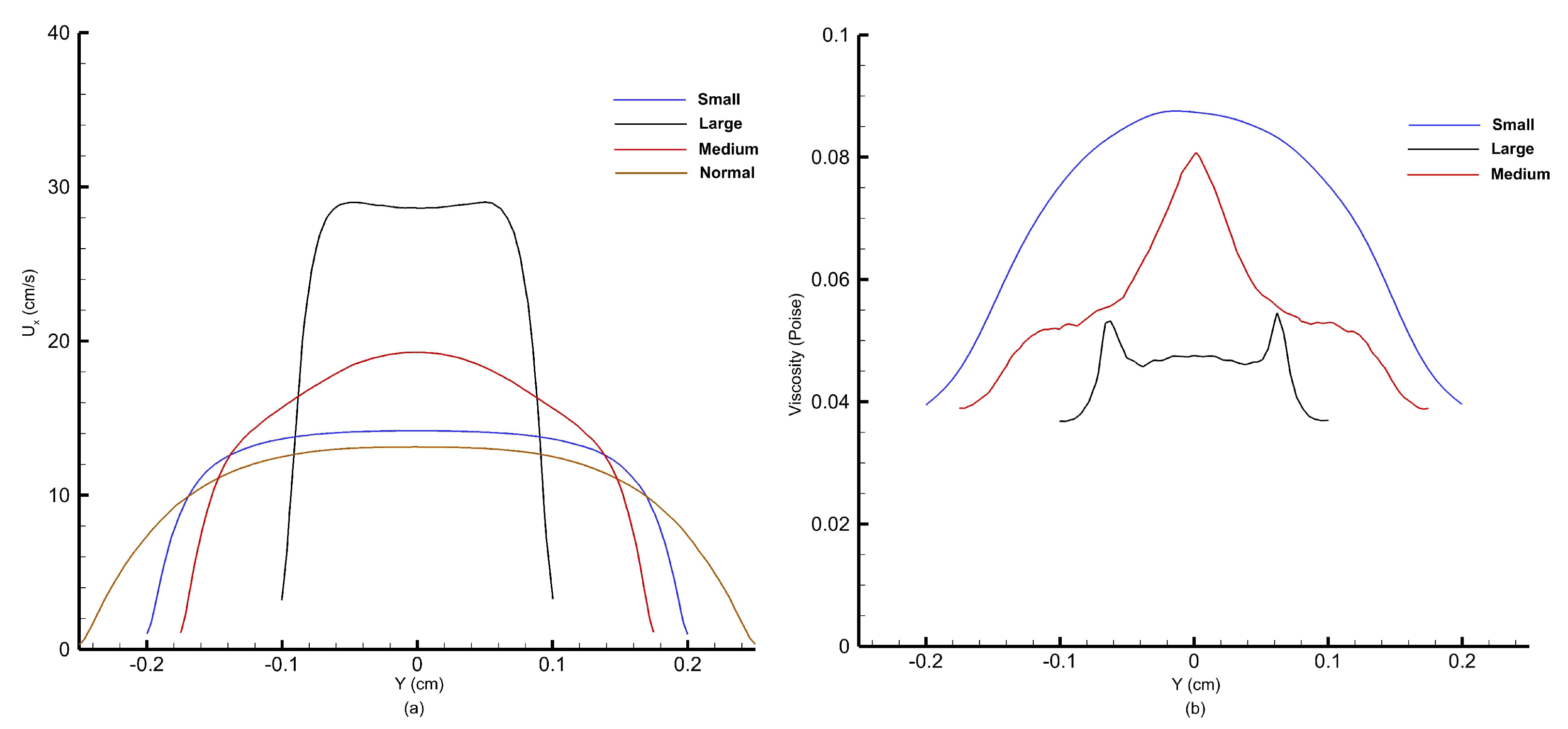
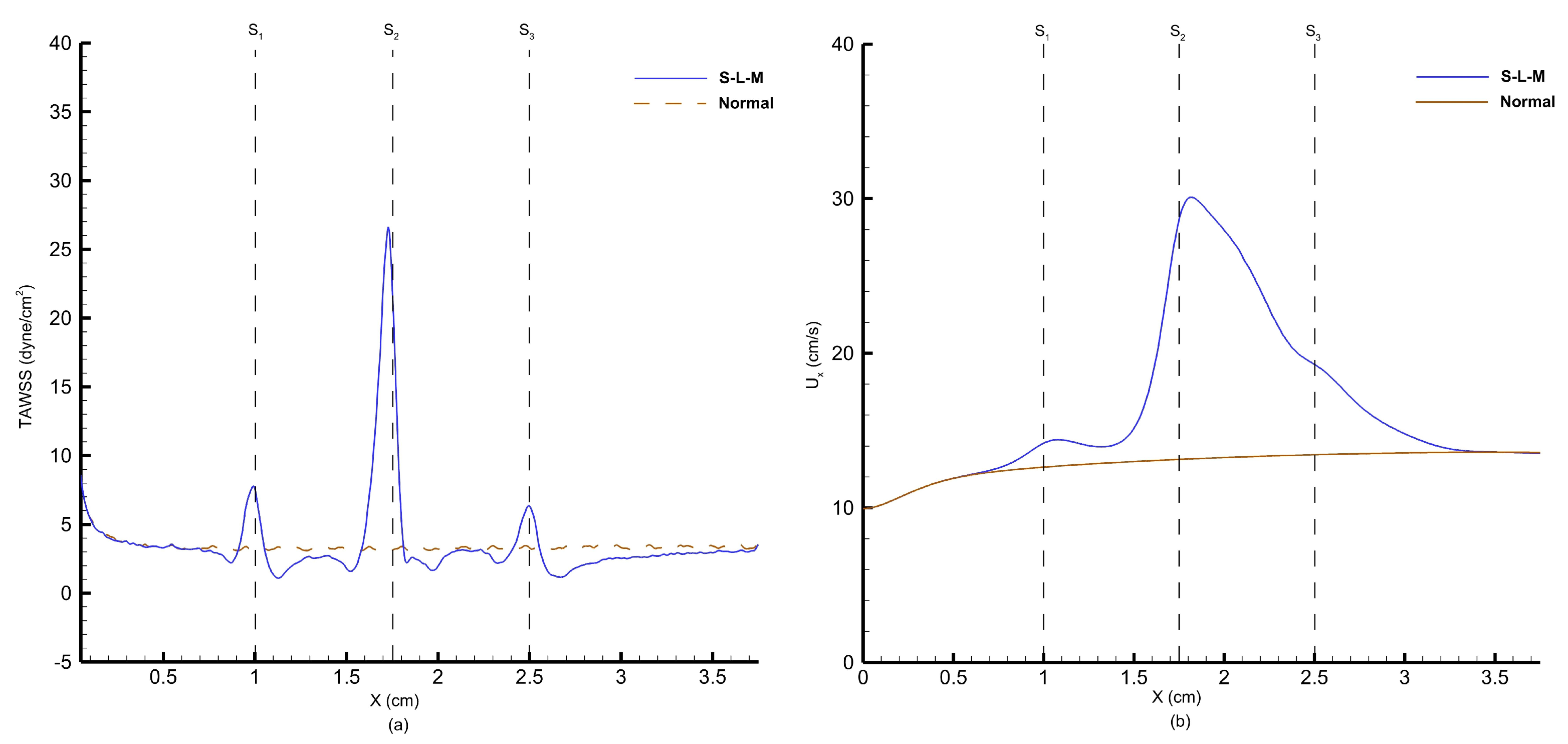
As mentioned above, the average flow velocity is inversely proportional to the cross-sectional area and as the flow approaches the stenosis, the cross-sectional area for the flow decreases, resulting in a rise in flow velocity. Figure 31 shows the velocity and viscosity profiles obtained at the peak of the cardiac cycle corresponding to systolic pressure. Figure 31a shows the velocity profiles, whereas Figure 31b shows the viscosity profiles obtained along the throat at three stenoses.

As observed from Figure 31a, as the percentage of stenosis increases, the peak velocity at the stenosis throat increases. At the peak of the cardiac cycle, blood flow velocity reaches 14 cm/s at the small stenosis, 19 cm/s at the medium stenosis, and almost 30 cm/s at the large stenosis, which is more than twice of that obtained for the normal artery without any stenosis. From Figure 31b, we obtain viscosity profiles that correspond to velocity profiles observed in Figure 31a. Viscosity is a measure of a fluid’s resistance to flow. It determines how easily a fluid deforms under shear stress. In the context of fluid flow, viscosity affects the velocity gradient within the fluid. This means that in regions where there is a high velocity gradient (such as near walls of the artery), viscosity resists the flow, resulting in viscous drag. Therefore, as the blood accelerates after encountering small, large, and medium stenoses, we observe a corresponding reduction in magnitude of viscosity. The viscosity, which depends on shear, decreases notably in the central region where shear is minimal. Consequently, the typically parabolic shape of the velocity profile becomes flattened at the center of the channel, which is what we have observed for velocity profiles at the throat of small and large stenoses.

The shear stress experienced by the arterial wall near a stenosis is significant, as it can provide insights into the mechanisms behind post-stenotic dilatation and contribute to understanding the development and progression of arterial stenosis. Figure 32a shows the time-averaged wall shear stress at the top wall. Changes in blood flow velocity occur within both the stenotic and post-stenotic zones due to alterations in the flow pressure gradient. Since wall shear stress is a function of velocity gradient and the highest velocity gradient occurs at the stenosis throat, we observe shear stress peaks as the flow accelerates across the stenosis. Referring to Figure 32a, as the flow encounters the small stenosis, we observe the first rise in wall shear stress that is proportional to the degree of small stenosis, following which shear stress reduces in the post-stenotic region. The largest peak in wall shear stress is observed for the large stenosis, where the velocity gradient is at its peak. Downstream of the large stenosis, the wall shear stress reduces to the normal value, and upon encountering the medium stenosis does in fact result in its rise again; however, this rise is not commensurate with the degree of medium stenosis, which was observed for small stenosis. From this observation, it is evident that large stenosis has affected the downstream flow dynamics. From Figure 32b, we can observe the rise in instantaneous centerline velocity at the peak of the cardiac cycle as the flow encounters multiple stenoses. Following the large stenosis, we observe a fall in centerline velocity, and after the medium stenosis, the velocity behavior is not altered.substantially.

Endothelial cells are the cells that form the inner lining of blood vessels, including arteries. They play a crucial role in maintaining the health and function of blood vessels. One of the factors that influence endothelial cell function is shear stress [66]. When blood flows smoothly and evenly along the vessel wall, shear stress is relatively constant. However, in case of a stenosed artery, high peak wall shear stress can lead to damage in the vessel wall, resulting in the thickening of the intima (the innermost layer of an artery), aggregation of platelets, and ultimately leading to thrombus (a blood clot) formation. Conversely, low shear stress in the region of flow separation is linked to mass transportation across the arterial wall and prolonged interaction time between platelets and endothelium. This increases the likelihood of atherosclerosis formation as the percentage of restriction in the artery increases.

In areas where blood flow is disturbed or chaotic, such as bends or downstream of stenosis, shear stress becomes oscillatory, meaning that it fluctuates in magnitude and direction rapidly over time. Endothelial cells respond differently to oscillatory shear stress compared to steady shear stress [67]. This behavior can be quantified with the help of the oscillatory shear index. OSI varies from 0 to 0.5 with 0 representing no oscillations or flow reversal, whereas 0.5 represents highly oscillatory flow behavior. A high OSI value is associated with areas of disturbed flow, which can result in endothelial cell dysfunction, leading to a higher risk of atherosclerotic plaque formation [67]. This is because the oscillatory nature of the shear stress can cause endothelial cells to promote inflammation within the artery walls and, subsequently, plaque formation. This plaque is made up of cholesterol, fatty substances, cellular waste products, calcium, and fibrin, and it can restrict blood flow through the arteries, leading to various cardiovascular problems like heart attacks and strokes.

Figure 33 shows the oscillatory shear index obtained along the top wall at small, large, and medium stenoses for the S-L-M configuration. As the blood flow follows the cardiac cycle depicted in Figure 27 and reaches the bottom of the cycle, corresponding to diastolic pressure, we observe a flow reversal. On top of that, the presence of multiple stenoses also induces recirculation regions in the immediate downstream of stenoses. This affects the instantaneous wall shear stress, which can be quantified using OSI. As shown in the figure above, before encountering the small stenosis, a normal flow is observed; however, as the small stenosis is encountered, OSI reduces in the converging section of the stenosis, whereas it rises sharply in the diverging section of the stenosis and in the downstream region of the stenosis. It is in the downstream of stenosis that a peak in OSI is observed where major flow reversal and recirculation is observed for large and medium stenoses. Major oscillations in wall shear stress are observed pre- and post-medium stenosis, indicating key regions of atherosclerosis progression.

Based on the above results, it is evident that downstream of stenoses, blood flow experiences flow recirculation and oscillatory wall shear stress, which prompts further plaque deposition aggravating the degree of blockage further. Another aspect that affects the flow dynamics is the presence of multiple stenoses such that one or more stenoses are present downstream of each other. This arrangement can affect blood flow behavior across each stenosis, either aggravating or suppressing plaque formation. Figure 33 indicates that the peak OSI value following the large stenosis is smaller than those obtained for medium stenosis. This phenomenon is likely due to the fact that, after a small stenosis, as the flow encounters a large stenosis, the velocity gradient changes abruptly, while the oscillations in wall shear stress do not change proportionally. On the other hand, high OSI coupled with low wall shear stress, at medium stenosis, is a crucial factor in the development, formation, and localization of atherosclerosis.

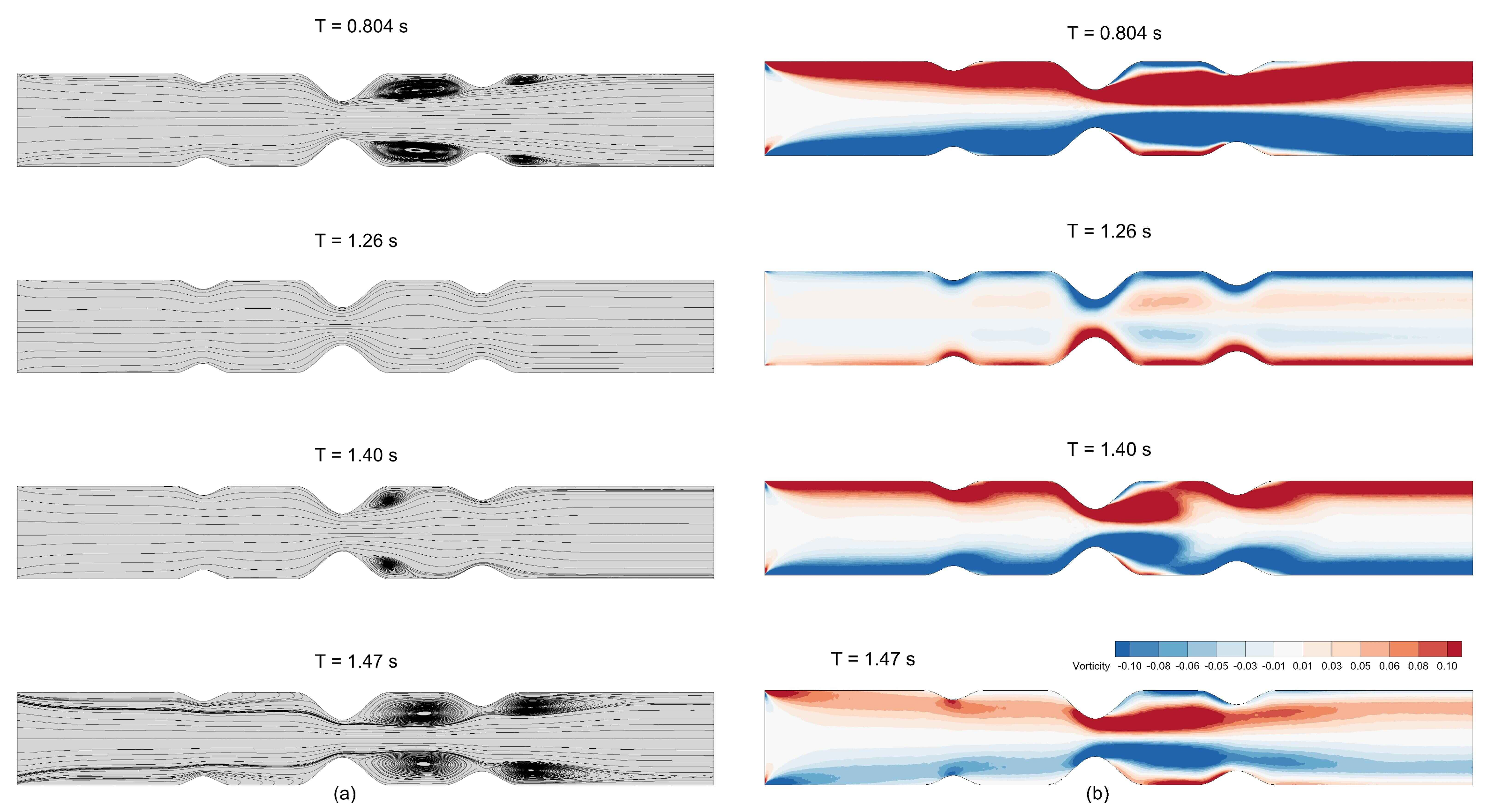
Figure 34a shows the streamlines obtained for blood flow through stenosed artery with S-L-M configuration at different time instances of the cardiac cycle, whereas Figure 34b shows the vorticity contours at the same time instances. At $T=0.804$ s, which represents the peak of the cardiac cycle, we observe major flow recirculation zones downstream of large and medium stenoses. At $T=1.26$ s, which represents the trough of the cardiac cycle, we observe a reversal in flow direction. Once the flow exceeds the trough of the cardiac cycle, it regains its normal flow direction and vortex strength, and vorticity magnitude increases as the cycle marches toward the peak of the cardiac cycle again. Major vortices are observed on both sides of the throat of the medium stenosis during the cardiac cycle. This signifies that this is the region of high intensity and fluctuations in wall shear stress and, thus, we observe two OSI peaks on both sides of the throat of the medium stenosis in Figure 33c.

The FV-iLBM solver presented in this study demonstrates significant potential for accurately simulating blood flow rheology in complex arterial vasculature. By combining the advantages of finite volume discretization with the incompressible lattice Boltzmann method, our approach effectively captures the non-Newtonian behavior of blood, particularly in regions of low shear rates and complex geometries. The solver’s ability to handle unstructured meshes and curved boundaries makes it particularly suitable for patient-specific simulations of arterial stenoses and aneurysms. Future studies will explore the impact of varying parameters in the Carreau model, specifically the relaxation time $\lambda$, on blood flow dynamics. Additionally, investigations into the effects of different Reynolds and Womersley numbers on blood flow in arteries afflicted with multiple stenoses and aneurysms will provide valuable insights into disease progression. These studies will also examine how various stenosis configurations and aneurysm sizes influence blood flow dynamics, contributing to a broader understanding of arterial disease development and progression.

4. Conclusions

This study presents a finite volume incompressible lattice Boltzmann method framework tailored to accurately capture hemodynamic behavior in complex vascular geometries. In the present study, we have addressed the inherent compressibility error associated with the standard lattice Boltzmann method while simulating incompressible flows. To mitigate this issue and enhance accuracy, an incompressible LBM model, proposed by Murdock and Yang [17], has been incorporated into the finite volume framework using the cell-centered finite volume approach. This approach leverages the simplicity of the LBM algorithm to simulate irregularly shaped flow domains using unstructured meshes. By leveraging unstructured meshes, the proposed framework effectively represents patient-specific arterial vasculature, ensuring an accurate reconstruction of arterial flow patterns. To ensure the accuracy and the robustness of our implementation, we have employed the linear reconstruction scheme for the reconstruction of distribution functions at cell interfaces. Boundary conditions have been implemented using the second-order accurate Non-Equilibrium Extrapolation method [35].

The FV-iLBM solver’s accuracy and versatility have been demonstrated through a range of benchmark simulations: it accurately captures velocity profiles in Taylor–Green vortex flow, shear wave attenuation, and developing flow through a 2D channel. Using the LR scheme, the method achieves second-order accuracy, and it consistently outperforms standard LBM when simulating pulsating flow such as Womersley flow. Furthermore, the FV-iLBM model has been shown to perform well in complex scenarios, such as lid-driven cavity flow, where it accurately reproduces velocity profiles and vortex characteristics, and external flow over NACA0012 airfoil, where predictions of pressure coefficient distribution, flow separation, and vortex shedding align closely with benchmark results, highlighting its suitability for both internal and external flow problems.

The FV-iLBM solver has been validated for simulating non-Newtonian blood flow using simulations of flows through a straight as well as a stenosed channel with the FV-iLBM model, accurately capturing the velocity and viscosity profiles. Simulating blood flow through a multi-stenosed artery demonstrates the FV-iLBM solver’s capability to effectively capture complex hemodynamic behaviors. The model accurately predicts viscosity and velocity profiles, as well as wall shear stress distribution, within the triple-stenosed artery. The presence of multiple stenoses leads to complex flow interactions, including flow acceleration, recirculation, and localized shear stress variations. Increased viscosity and a flattened velocity profile along the core, resulting from low shear rates, capture the non-Newtonian characteristics of blood flow in these constricted regions. Additionally, the velocity and wall shear stress profiles exhibit expected trends, with peaks at each stenosis throat, followed by regions of flow separation and reattachment, consistent with the principles of incompressible fluid dynamics. These results underscore the FV-iLBM solver’s potential for providing detailed insights into cardiovascular flow conditions, crucial for understanding the progression of diseases like atherosclerosis and aneurysms.