1. Introduction
The Empirical Bayes analysis uses a conjugate prior model, estimating hyperparameters from observations and using this estimate as a conventional prior for further inference [
1,
2]. It should be noted that prior distribution remains unknown because of the unknown hyperparameters. However, marginal distribution could be employed to recover the prior distribution based on observed data. For further literature about empirical Bayes, researchers are referred to [
1,
3,
4,
5,
6,
7,
8,
9,
10].
The motivations behind this paper could be summarized below. Firstly, to our knowledge, no one in the empirical Bayes analysis literature has considered the exponential-inverse gamma model. Additionally, as highlighted by [
11], when dealing with a parameter space
in the location case, it is appropriate that the squared error loss equally penalizes both overestimation and underestimation. However, in cases where we have a restricted positive space of parameters
with lower bound setting at 0 as well as an asymmetric problem of estimation, selecting Stein’s loss [
12,
13] instead of squared error loss is more suitable since it equally penalizes both gross overestimation and underestimation—actions that tend towards 0 or ∞ will incur infinite losses. In our specific context of the exponential-inverse gamma model (
1), where our interested parameter is
representing a mean parameter value, we opt for Stein’s loss. Relevant literature on Stein’s loss can be found for interested readers [
9,
14,
15,
16].
The key findings of this paper are outlined below. First of all, the Bayes estimator of the mean parameter for the exponential distribution is derived under Stein’s loss, and its Posterior Expected Stein’s Loss (PESL) is calculated within an exponential-inverse gamma model. Additionally, we obtain a Bayes estimator of a mean parameter using squared error loss as well as its associated PESL. Furthermore, we employ two methods, namely the method of moments and the method of Maximum Likelihood Estimation (MLE), to estimate a mean parameter of an exponential distribution, which is assumed with a prior distribution of inverse gamma in an empirical Bayes framework. In our simulations, we investigate five aspects. The simulations suggest that MLEs are superior to moment estimators in estimating hyperparameters. At last, we illustrate our theoretical studies by applying them to analyze Static Fatigue 90% Stress Level data.
The remaining part of the paper is structured below. In
Section 2, four theorems will be presented.
Section 3 will provide an illustration of five aspects in simulations. In
Section 4, we employ the Static Fatigue 90% Stress Level data to demonstrate the empirical Bayes estimators’ calculations for a mean parameter of an exponential distribution with an inverse gamma prior. Finally,
Section 5 offers conclusions and discussions.
2. Main Results
The exponential-inverse gamma model is assumed to generate observations
in our study:
The hyperparameters
and
need to be estimated, while
represents a parameter of interest that is unknown.
denotes an exponential distribution with a mean parameter of
, and
denotes an inverse gamma distribution characterized by two hyperparameters. According to [
1], when observing data
, statisticians aim to make inferences about
. Therefore,
directly provides information regarding the parameter
, while
Supplementary Information also offered. A relationship between the primary data
as well as
Supplementary Information is established through their common distributions
and
.
There are two probability density function (pdf) forms for the exponential distribution. One form uses the mean (or scale)
as the parameter (see [
11]), and
with pdf
, for
and
. Another form utilizes the rate
as the parameter (see [
2,
17]), and
with pdf
, for
and
. The two pdfs are the same with a relationship of the parameters
.
Other distributions that have two alternative forms are the gamma and inverse gamma distributions. Similar to [
18], suppose that
and
. The pdfs of
X and
Y are, respectively, given by
Moreover, suppose that
and
. The pdfs of
and
are, respectively, given by
The exponential-gamma model is assumed to generate observations
:
Firstly, the exponential-inverse gamma model (
1) and the exponential-gamma model (
2) are equivalent in the sense of their marginal pdfs. For convenience, now let
,
,
,
,
, and
be random variables with the corresponding distributions. For example,
is a random variable with the
distribution. It is easy to see that
Therefore, the two hierarchical models (
1) and (
2) are equivalent. It is straightforward to derive that the two marginal pdfs of the two hierarchical models are the same, and they are equal to
Since the two marginal pdfs are the same, the moment estimators (displayed in Theorem 2) and the MLEs (see Theorem 3) of the hyperparameters
and
for the two hierarchical models (
1) and (
2) are the same.
Another reason to use (
1) is that it motivates us to consider 16 hierarchical models of the gamma and inverse gamma distributions (see [
18]). It is easy to see that
is a conjugate prior for the
distribution. Writing in the form of likelihood-prior, it is
. Similarly, the
is a conjugate prior for the
distribution. Writing in the form of likelihood-prior, it is
. The
expression motivates us to consider
,
,
, and
as the likelihood, and
,
,
, and
as the prior, leading to 16 combinations of the likelihood-prior.
The introduction highlights the importance of calculating and utilizing a Bayes estimator for a mean parameter
under Stein’s loss, considering a prior
. This particular estimator is denoted as
. The supplement provides further justifications for why Stein’s loss outperforms squared error loss on a restricted positive space of parameters
. For clarity, Stein’s loss function is given by
while the squared error loss function is given by
2.1. Bayes Estimators and PESLs
In the exponential-inverse gamma model, the following theorem provides a summary of the posterior of and a marginal distribution of X. The proof of the theorem can be found in the supplement.
Theorem 1. The posterior of for the exponential-inverse gamma model is obtained asin which The marginal distribution of X, furthermore, is Two inequalities will be derived for any hierarchical model, assuming the existence of posterior expectations. The same as [
15], under Stein’s loss, a Bayes estimator of
is
and under squared error loss, a Bayes estimator of
is
The same as [
15], we can show that
by leveraging the application of Jensen’s inequality. The same as [
15], the PESL at
is
The PESL at
is
The following should be noted
This is a straightforward result of a method for deriving a Bayes estimator, because is constructed to minimize the PESL.
The Bayes estimators
and
, as well as the PESLs
and
, are analytically calculated under the exponential-inverse gamma model. According to (
3), we possess
The Bayes estimator of
is elegantly expressed by the following equation under Stein’s loss (reminiscent of [
15])
in which
and
are determined by (
4). Additionally, under squared error loss, we obtain
It can be observed that
which illustrates the theoretical investigation in (
6). The analytical calculation of
and
requires the analytical calculation of
, which is given by
in which
is a digamma function. The PESL at
and
can be obtained through algebraic operations, similar to the approach presented in [
15],
and
The demonstration of this fact is straightforward
The sentence exemplifies the theoretical investigation of (
7). Notice that the PESLs solely depend on
, disregarding
. Hence, the dependency of the PESLs lies exclusively on
, without considering
and
. In both simulations and real data sections, we will provide examples illustrating (
6) and (
7). Furthermore, we shall demonstrate that the dependence of the PESLs is solely on
, excluding any influence from
and
.
The Bayes estimators, as well as the PESLs considered in this subsection, assume prior knowledge of the hyperparameters
and
. In other words, the PESLs and Bayes estimators presented here are computed using the oracle method, which will be further discussed in
Section 2.3.
2.2. Empirical Bayes Estimators of θn+1
Empirical Bayes estimators of
can be obtained by estimating the hyperparameters from the
Supplementary Information . There are two commonly used methods for estimating the hyperparameters: the method of moments and the method of MLE.
The method of moments offers estimators for the hyperparameters of the exponential-inverse gamma model, and their consistencies are succinctly summarized below. The proof of the theorem can be found in the supplement.
Theorem 2. The hyperparameters of an exponential-inverse gamma model can be estimated using the method of moments, where Here, , represents X’s kth sample moment. Additionally, it should be noted that the moment estimators exhibit consistency as estimators for these hyperparameters.
The estimators of hyperparameters for the exponential-inverse gamma model, obtained through the method of MLE, are presented below, along with an overview of their consistent properties. The proof of the theorem can be found in the supplement.
Theorem 3. The hyperparameters’ estimators of an exponential-inverse gamma model obtained through the method of MLE, denoted as and , are determined by solving equations: Furthermore, it is worth noting that these MLEs serve as consistent estimators.
It is infeasible to analytically calculate the MLEs for
and
through solving nonlinear Equations (
12) and (
13), necessitating the utilization of numerical solutions. Newton’s method can be employed to solve Equations (
12) and (
13) and find the MLEs. It should be noted that the MLEs exhibit a high degree of sensitivity to initial estimates; thus, moment estimators are commonly utilized as reliable initial estimates.
The estimators of the parameter in the exponential-inverse gamma model are enhanced through empirical Bayes methodology, obtained through both moment and MLE methods, and they are summarized below.
Theorem 4. Under Stein’s loss and using the method of moments, the empirical Bayes estimator of the parameter in the exponential-inverse gamma model is (8) with estimated hyperparameters according to Theorem 2. Alternatively, when employing the MLE method and under Stein’s loss, the empirical Bayes estimator of the parameter in the exponential-inverse gamma model is (8) with numerically determined hyperparameters as stated in Theorem 3. Remark 1. In Theorem 4 and under Stein’s loss, the empirical Bayes estimator of the parameter in the exponential-inverse gamma model is given by (8), where the hyperparameters are estimated from observed data through marginal likelihood. More specifically, using the method of moments, the hyperparameters are estimated from observed data according to Theorem 2. Alternatively, when employing the MLE method, the hyperparameters are numerically determined from observed data as stated in Theorem 3. 2.3. Theoretical Analysis of PESLs and Bayes Estimators of Three Methods
PESLs and Bayes estimators for three methods (oracle, moment, and MLE) will be theoretically compared in this subsection. It is worth noting that their numerical comparisons can be found in the supplement.
Subscripts 0, 1, and 2 correspond to oracle, moment, and MLE, respectively. Following calculations as before [
9,
15], the PESLs of these three methods are given by (
)
in which
The hyperparameters are unknown, while the moment estimators of and in Theorem 2, and the numerically determined MLEs of and in Theorem 3, are presented.
Under Stein’s loss, a Bayes estimators of
minimize an associated PESL (see [
1,
11,
15]), i.e.,
in which
represents a space of actions. Herein
a is an action (estimator),
denotes Stein’s loss, and
refers to the unknown interested parameter. The Bayes estimators can be easily derived in a manner similar to [
15]:
The PESLs at
for
exhibit similarities to those discussed in Zhang’s work [
15]:
Under squared error loss, a Bayes estimators of
are provided in a similar manner as described by [
15]:
for
. Additionally, the PESLs at
can be derived in a manner similar to that of [
15] for
:
The primary objectives of our study involve estimating the PESLs and Bayes estimators using the method of oracle. However, the hyperparameters remain unknown. The method of oracle possesses knowledge of these hyperparameters only in simulations, whereas in reality, they are undisclosed.
The positive aspect is that the PESLs and Bayes estimators can be obtained through the method of moments and method of MLE once the data are provided. To compare the moment and MLE methods in simulations, we can assess the PESLs and Bayes estimators generated by these two methods against those obtained using the method of oracle. In simulations, the method that yields PESLs and Bayes estimators closer to those derived from the method of oracle is considered superior.
3. Simulations
We conduct simulations to examine the exponential-inverse gamma model (
1) in this section. We present five key aspects of our findings. Firstly, we demonstrate an inequality (
6) of Bayes estimators and an inequality (
7) of PESLs using the method of oracle. Secondly, we show that both moment estimators and MLEs consistently estimate hyperparameters. Thirdly, we calculate the model’s goodness-of-fit with respect to simulated data. Fourthly, we compare numerically the PESLs and Bayes estimators obtained from three methods: oracle, moment, and MLE. Finally, the model’s marginal densities are plotted for different hyperparameters.
The simulated data are produced based on the model (
1), with hyperparameters set as
and
. These values are selected because the conditions
and
are necessary for the moment-based estimation of the hyperparameters. Alternative numerical values for the hyperparameters can also be defined.
3.1. Two Inequalities Related to Bayes Estimators and PESLs
In this subsection, we aim to demonstrate numerically the two inequalities (
6) and (
7) related to Bayes estimators and PESLs using the oracle approach.
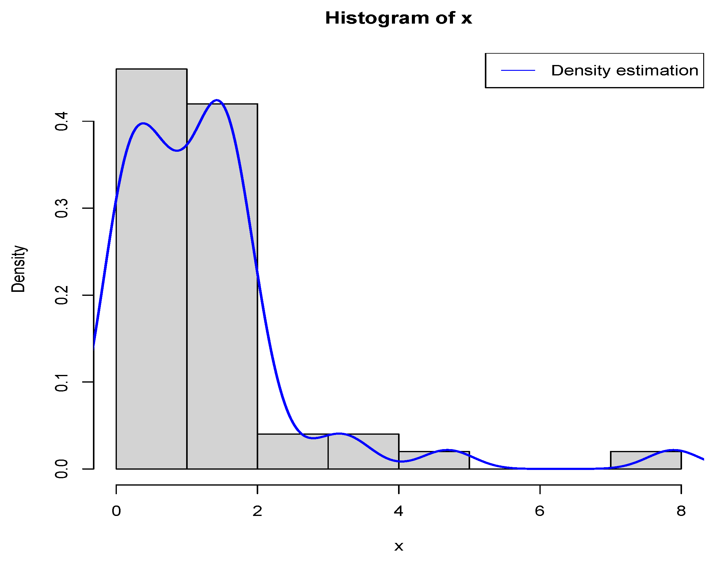
First, we fix
,
, and
.
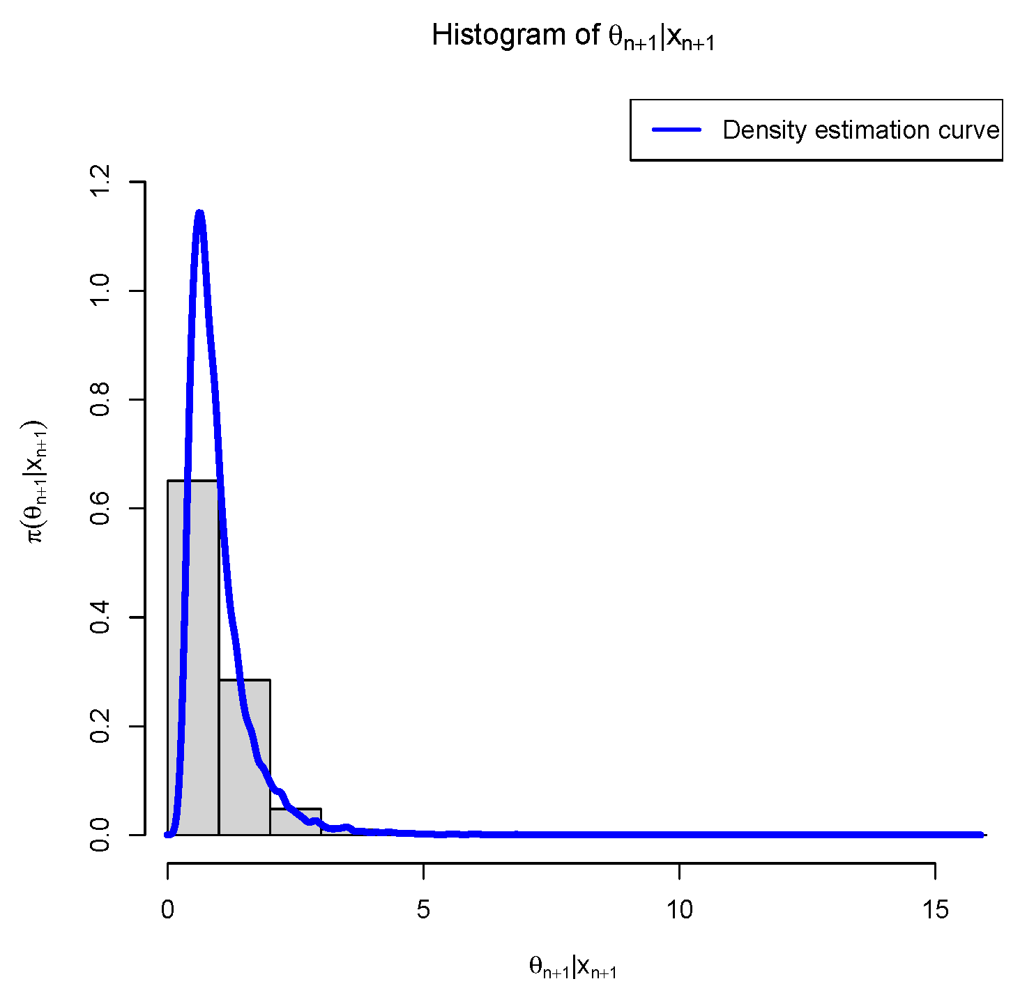
Figure 1 presents the histogram for
along with the estimated density curve of
. Our goal is to determine
in a way that minimizes the PESL based on
. Numerical results show that
and
which exemplify the theoretical studies of (
6) and (
7).
Next, consider allowing one of the variables
,
, or
to vary while keeping the others constant. As depicted in
Figure 2, both the Bayes estimators and the PESLs are represented as functions of
,
, and
. From the left panels of the figure, it is evident that the Bayes estimators are influenced by
,
, and
, illustrating the relationship (
6). More precisely, the Bayes estimators decrease with increasing
, increase linearly with
, and also increase linearly with
. On the other hand, the right panels reveal that the PESLs are solely dependent on
, showing no dependence on
or
, thus exemplifying the inequality (
7). Specifically, the PESLs exhibit a decreasing trend as
increases. In conclusion, the findings presented in
Figure 2 validate the theoretical analyses outlined in (
6) and (
7).
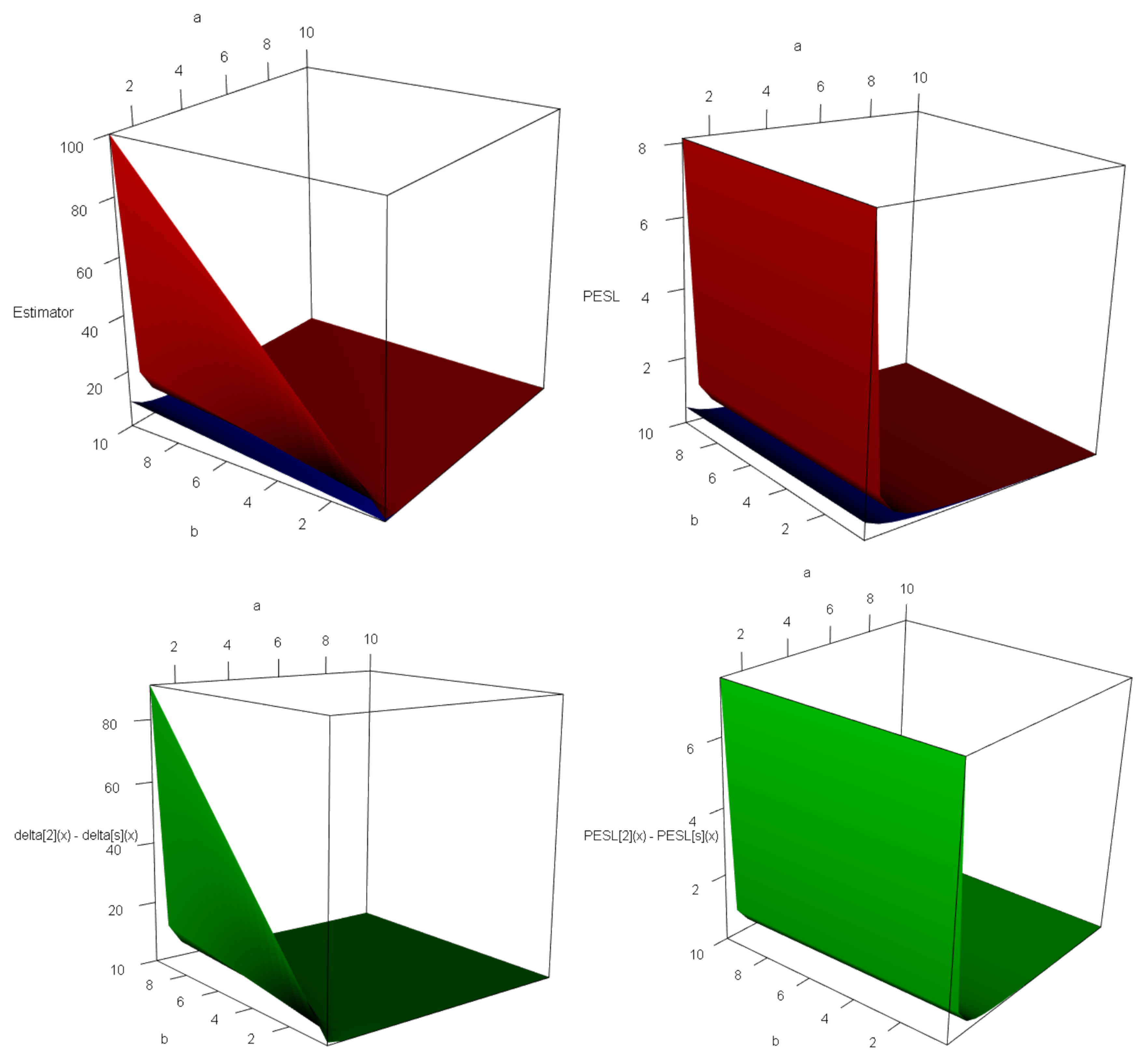
Third, given that the Bayes estimators
and
, as well as the PESLs
and
, rely on
and
, where
and
, we can visualize their surfaces over the domain
using the ‘persp3d()’ function from the R (1.0) package ‘
rgl’ (see [
16,
19]). It is worth noting that while the ‘persp()’ function in the R package ‘
graphics’ cannot overlay additional surfaces onto an existing one, ‘persp3d()’ has this capability. Furthermore, ‘persp3d()’ enables users to rotate the perspective plots of the surfaces according to their preferences.
Figure 3 displays the surfaces of the Bayes estimators and the PESLs, along with the surfaces representing the differences between these estimators and PESLs. From the first two plots on the left, it is evident that
for all
in
D. Similarly, the last two plots on the right indicate that
for all
in
D. The findings presented in
Figure 3 align with the theoretical results outlined in (
6) and (
7).
3.2. Consistencies of Moment Estimators and MLEs
In this subsection, we aim to demonstrate through numerical examples that both the moment estimators and the MLEs serve as consistent estimators for the hyperparameters
and
of the hierarchical exponential and inverse gamma model (
1). It is important to note that in this subsection, only the data
are utilized.
The estimators for the hyperparameters ( and ) based on the method of moments and MLE are denoted as ( and ) and ( and ), respectively. Consistency implies that converges to in probability as n approaches infinity, and converges to in probability as n approaches infinity, for . Here, corresponds to the moment estimator, and corresponds to the MLE.
Let
represent either hyperparameter
or
. Then, consistency can be expressed as
converging to
in probability as
n tends to infinity, for
. Alternatively, consistency means that for every
and every
, the following holds:
The probabilities can be approximated by their corresponding frequencies:
for
, where
is the indicator function of
A, equaling 1 if
A is true and 0 otherwise, and
M represents the number of simulations. Thus, the convergence of the frequencies (
, with
being
or
, and
) toward 0 indicates that the estimators are consistent.
The occurrences of the moment estimators (
and
) and the MLEs (
and
) for the hyperparameters (
and
) as
n changes, given
and
,
, and
, are presented in
Table 1. By examining
Table 1, we can identify the following observations.
For values of 1, 0.5, or 0.1, the frequencies of the estimators, denoted as where or and , approach 0 as n grows toward infinity. This indicates that both the moment estimators and the MLEs are consistent estimators for the hyperparameters. When is set to 0.1, the frequencies of these estimators remain relatively high. Nevertheless, we can still observe a decreasing trend toward 0 as n increases to infinity.
By examining the frequencies associated with
, 0.5, and 0.1, it can be seen that as
decreases, the frequencies become higher. This occurs because the conditions
become simpler to satisfy.
By comparing the moment estimators with the MLEs for the hyperparameters and , it can be observed that the frequencies of the MLEs are lower than those of the moment estimators. This indicates that the MLEs outperform the moment estimators in terms of consistency when estimating the hyperparameters.
3.3. Model Fit Assessment: Kolmogorov–Smirnov Test
In this subsection, we aim to evaluate how well the hierarchical exponential and inverse gamma model (
1) fits the simulated data (see [
9,
20,
21]). It is important to note that in this subsection, we only utilize
. Typically, the chi-square test serves as an indicator of fit quality. Nevertheless, due to its high sensitivity—stemming from challenges in determining the number of groups and identifying appropriate cut-points—we opt for an alternative approach. Instead of relying on the chi-square test, we will employ the Kolmogorov–Smirnov test (KS test) to assess the goodness-of-fit.
The Kolmogorov–Smirnov (KS) statistic is defined as the maximum distance
D between the empirical cumulative distribution function (cdf), denoted as
, and the theoretical population cdf,
. Mathematically, this can be expressed as
In the R programming environment, the KS test can be performed using the built-in function ‘ks.test()’, as detailed in references such as [
22,
23,
24]. It is important to note that the KS test is primarily applicable for one-dimensional continuous distributions. However, adaptations of the KS test for discrete data have also been explored in recent literature, including works by [
25,
26,
27].
In the context of our study, the null hypothesis assumes that the random variable
X follows an exponential-inverse gamma distribution with parameters
and
, written as
. The
represents the marginal distribution derived from the hierarchical exponential and inverse gamma model (
1). The marginal density of the
distribution, as given in (
5), is clearly one-dimensional and continuous. Consequently, the KS test serves as a suitable tool for assessing the goodness-of-fit in this scenario.
The outcomes of the KS test for assessing the goodness-of-fit of the model (
1) to the simulated data are presented in
Table 2. It is important to note that the data were generated based on the hierarchical exponential and inverse gamma model (
1) with parameters
and
. In this table, the hyperparameters
and
are estimated using three distinct approaches. The first approach is the oracle method, where the true values of the hyperparameters
and
are known. The second approach is the moment estimation method, in which
and
are estimated using their respective moment estimators (as described in Theorem 2). The third approach is the MLE method, where
and
are estimated using their MLEs (as outlined in Theorem 3). In this table, the sample size is set to
, and the number of simulations conducted is
. To evaluate the performance, we employ five metrics proposed in [
9]:
,
, (min
D)%, (max
p-value)%, and
. Here,
represents the average
D values (
14) across
M simulations, with smaller values indicating better performance. The
denotes the average
p-values from
M simulations, where larger values are preferred. (min
D)% refers to the proportion of
M simulations in which the minimum
D value is achieved among the three methods, with higher percentages being more favorable. The sum of the three (min
D)% values should equal 1. (max
p-value)% indicates the percentage of
M simulations where the maximum
p-value is attained among the three methods, with higher percentages also being desirable. Similarly, the sum of the three (max
p-value)% values should equal 1. Lastly,
reflects the proportion of
M simulations in which the null hypothesis
(defined as
p-value
) is accepted for each method, with high values being preferable. Each
value should fall within the range of 0–100%.
By examining
Table 2, the following observations can be made.
The
values obtained using the three methods are 0.0270, 0.0230, and 0.0205, respectively. This indicates that the MLE method performs the best, followed by the moment method as the second-best, while the oracle method ranks last. One plausible explanation for this outcome is that in (
14), the empirical cdf
relies on data, and the population cdfs
for both the MLE and moment methods also depend on data. In contrast, the population cdf
for the oracle method does not rely on data.
The corresponding to the three methods are 0.5102, 0.6683, and 0.7693, respectively. These results align with the previous findings, ranking the MLE method first, the moment method second, and the oracle method third. The explanation for this phenomenon has been discussed in the preceding paragraph.
The (min D)% values for the three methods are 0.16, 0.15, and 0.69, respectively. Notably, the (min D)% value of the MLE method represents more than half of the M simulations. Based on these results, the order of preference among the three methods is the MLE method, the oracle method, and the moment method.
The (max p-value)% values for the three methods are also 0.16, 0.15, and 0.69, respectively. A smaller D value corresponds to a larger p-value, meaning the smallest D value correlates with the largest p-value. Consequently, the (min D)% and (max p-value)% values for the three methods are identical. Thus, the preferred order remains the MLE method, the oracle method, and the moment method.
Finally, the values for the three methods are 0.97, 0.99, and 1.00, respectively. Once again, the ranking of the methods in terms of preference is the MLE method, the moment method, and the oracle method.
Figure 4 presents the boxplots of
D values for the three methods (on the left) and the boxplots of
p-values for the three methods (on the right). Based on this figure, we can identify the following observations.
The D values obtained using the oracle method are considerably higher than those of the other two methods. Given that smaller D values are preferable, the ranking of the three methods in terms of performance is: the MLE method, followed by the moment method, and lastly the oracle method.
Additionally, the p-values of the oracle method are notably lower than those of the other two methods. Since larger p-values are more desirable, the preference order for the three methods based on p-values remains the same: the MLE method, the moment method, and finally the oracle method.
It is also worth noting that there is an inverse relationship between D values and p-values; smaller D values correspond to larger p-values, while larger D values result in smaller p-values.
Overall, the MLE method outperforms the moment method in both D values and p-values.
3.4. Numerical Comparisons Between Bayes Estimators and PESLs of Three Methods
In this subsection, we will conduct a numerical comparison of the Bayes estimators and PESLs for three approaches: the oracle method, the moment method, and the MLE method. It should be highlighted that the theoretical comparisons among these three methods regarding their Bayes estimators and PESLs are presented in
Section 2.3.
It is important to highlight that the data have been generated based on the hierarchical exponential and inverse gamma model (
1), using
and
. Additionally, the oracle method is aware of the hyperparameters
and
during the simulation process.
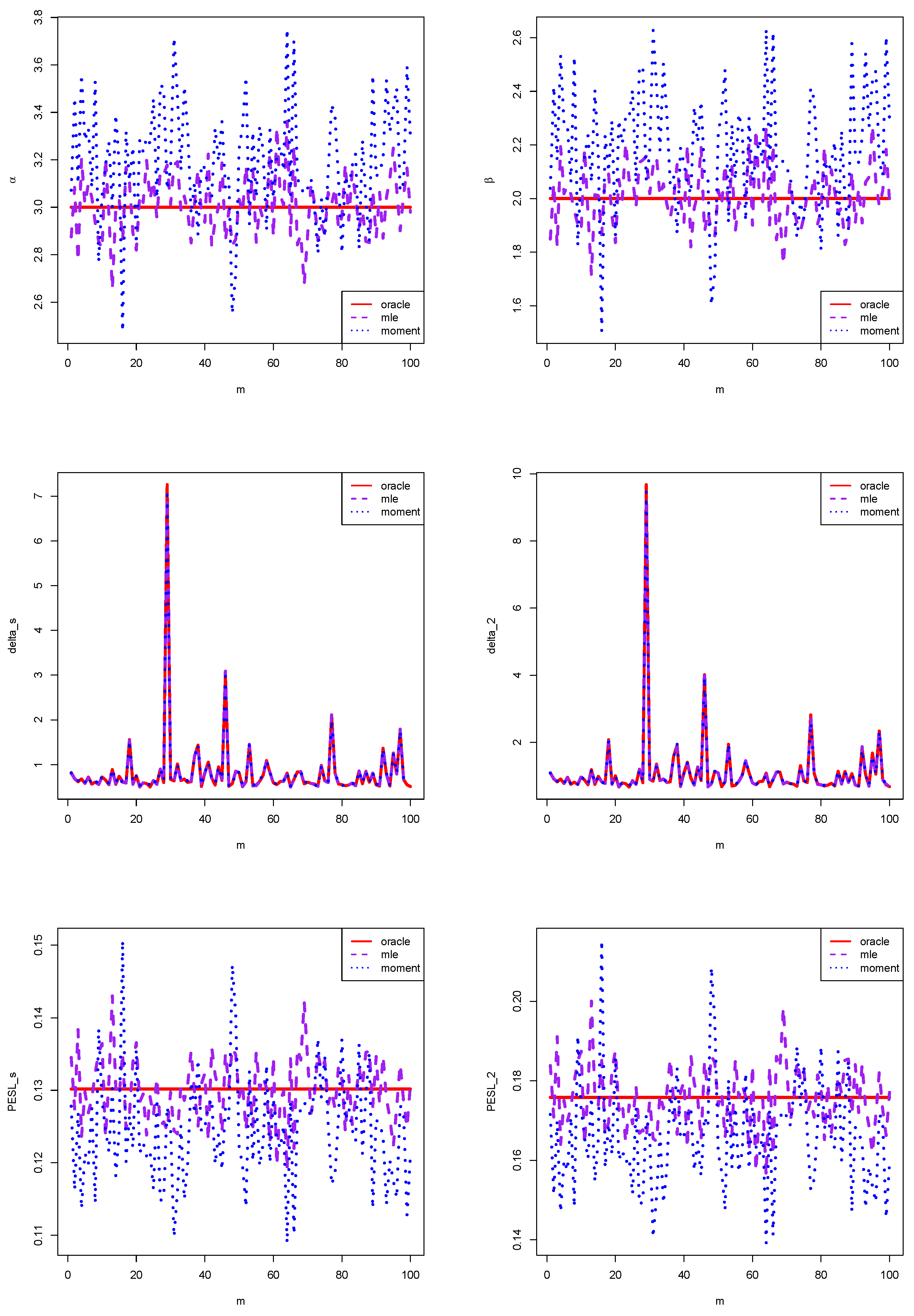
The comparisons of
,
,
,
,
, and
for the three methods, given a sample size of
and a number of simulations
, are presented in
Figure 5. By examining the figure, we can identify that the MLE method demonstrates superior performance compared to the method of moments in several aspects. Specifically:
For the estimators of and , the MLE approach aligns significantly closer with the oracle method than the moment method.
Regarding the Bayes estimators and , the MLE method exhibits a slight advantage over the moment method in terms of proximity to the oracle method. The differences among these estimators are minimal, making their respective curves nearly indistinguishable.
In the context of the PESL functions and , the MLE method again shows a marked improvement over the moment method in its alignment with the oracle method.
Overall, the graphical results consistently suggest that the MLE method outperforms the moment method, as demonstrated by the hyperparameter estimators, Bayes estimators, and PESL values obtained through the MLE method being more consistent with those derived from the oracle method than those from the moment method.
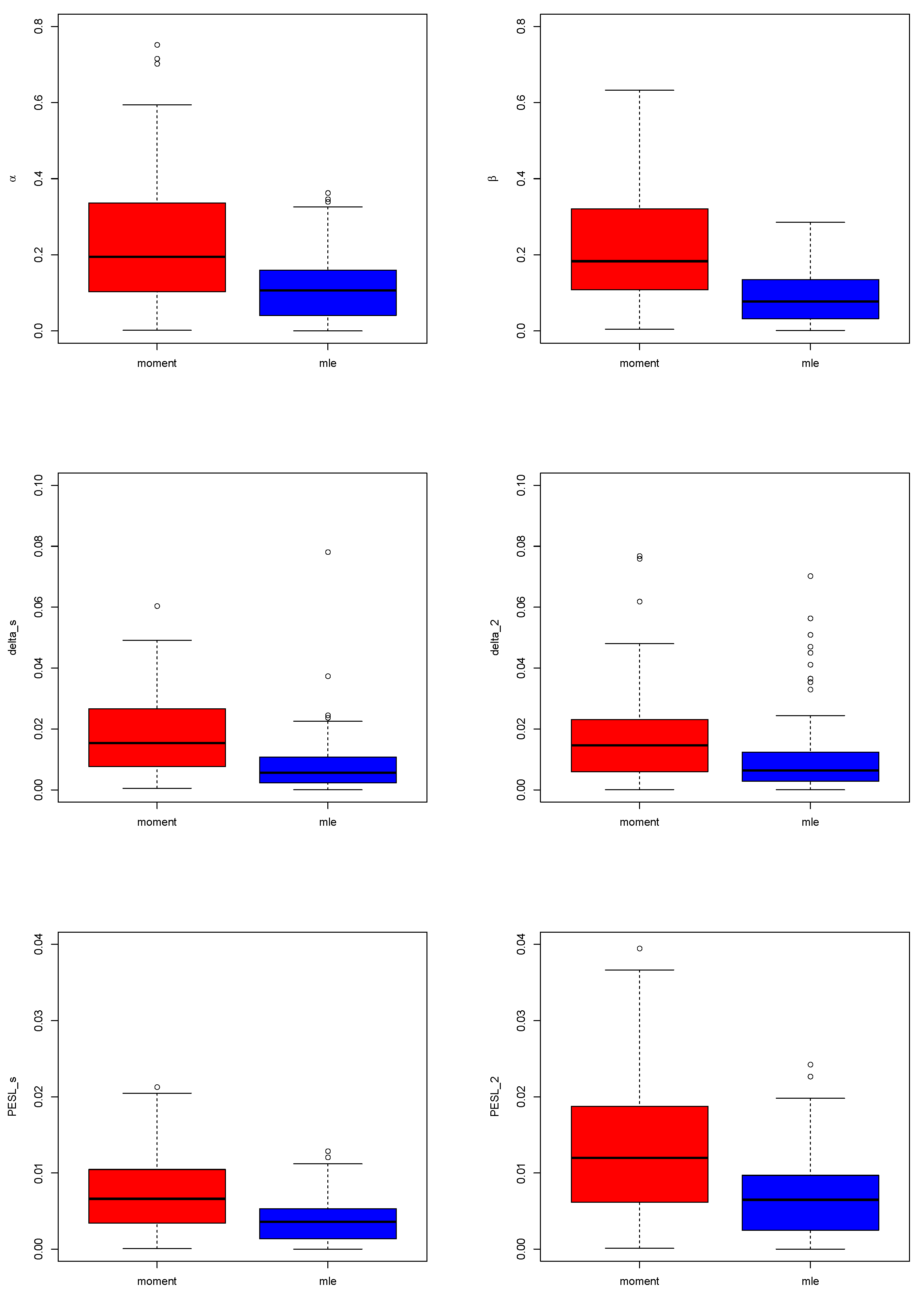
Figure 6 presents the boxplots of absolute errors obtained using the oracle method for both the moment method and the MLE method, with a sample size of
and
simulations. The visualizations consistently demonstrate that the MLE method outperforms the moment method. This is because the absolute errors associated with the oracle method for the hyperparameter estimators, Bayes estimators, and PESLs are significantly smaller when using the MLE method compared to the moment method.
The summary of the averages and proportions of absolute errors for the oracle method, using both the moment method and the MLE method, is presented in
Table 3. Specifically, these averages represent the sample means of the absolute error vectors derived from the oracle method via the moment and MLE methods, where smaller values indicate superior performance. The proportions reflect the sample ratios of absolute errors achieved by each method that are equal to the minimum value between the two methods, with higher proportions being more desirable. From the table, it can be observed that the MLE method yields significantly smaller average absolute errors compared to the moment method. Additionally, the proportions of absolute errors obtained through the MLE method are notably larger than those from the moment method. Overall, the data in the table demonstrates that the MLE method outperforms the moment method in terms of both the averages and proportions of absolute errors as determined by the oracle method.
Let
equal
or
. Suppose
represents an estimator of
, where
corresponds to the method of moments estimator and
corresponds to the MLE. The Mean Square Error (MSE) for the estimator
is given by (as referenced in [
11]):
In a similar manner, the Mean Absolute Error (MAE) for the estimator
is defined as (also from [
11]):
It is important to note that both MSE and MAE serve as criteria for comparing two distinct estimators. These metrics function as risk functions (or expected loss functions) associated with the estimators of hyperparameters, providing a measure of the estimators’ performance. Generally, smaller values of MSE and MAE indicate superior performance of the estimator.
The MSE and MAE for the hyperparameter estimators using both the moment method and the MLE method are presented in
Table 4. As shown in the table, when estimating the hyperparameters
and
, the MLE method significantly outperforms the moment method, since the MSE and MAE values obtained via the MLE method are considerably lower than those achieved through the moment method.
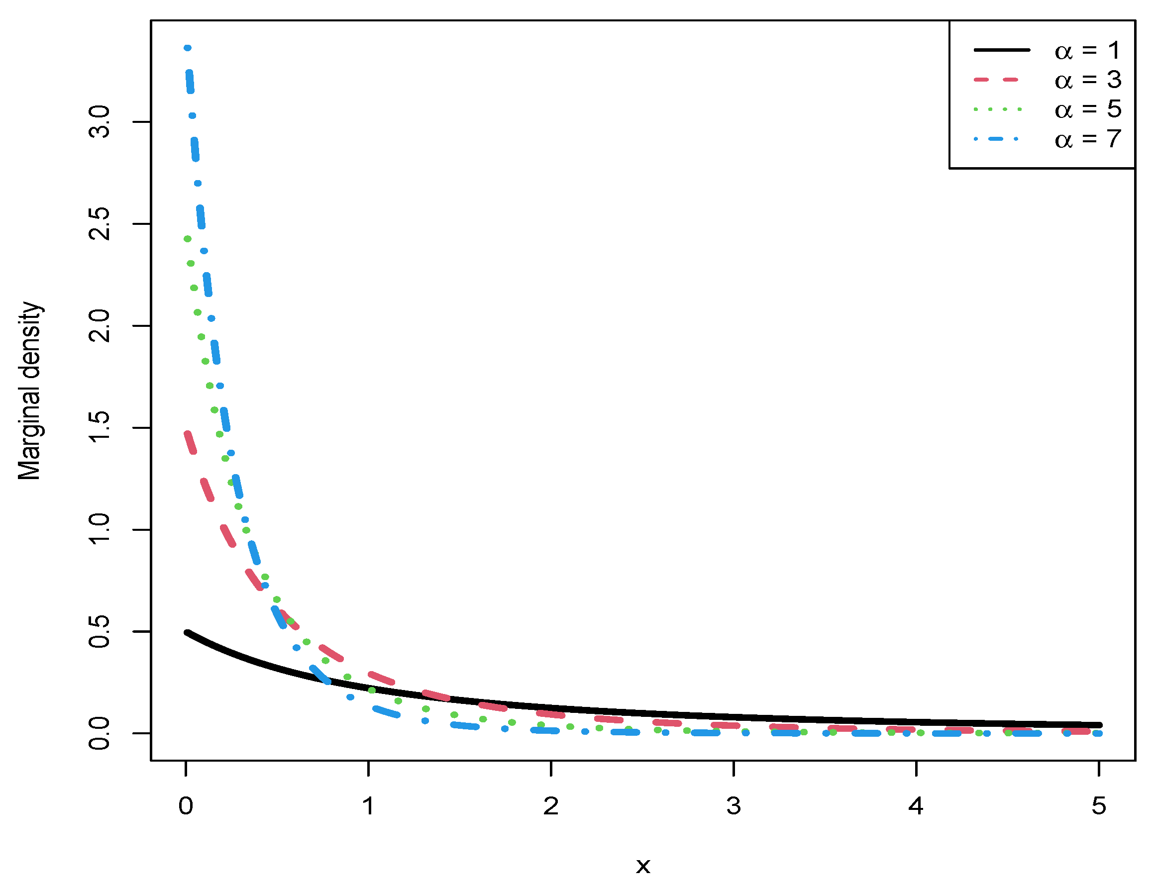
3.5. Marginal Densities for Different Hyperparameters
In this subsection, we aim to illustrate the marginal densities of the hierarchical exponential and inverse gamma model (
1) using different hyperparameters
and
. It is important to note that the marginal density of
X is defined by (
5), which depends on the two hyperparameters
and
. Here, we will investigate the variations in the marginal densities in relation to the density where the hyperparameters are set as
and
. Additionally, other specific values for the hyperparameters can also be considered.
Figure 7 illustrates the marginal densities for different values of
(
), with
remaining constant at 2. As observed in the figure, an increase in
corresponds to a higher peak value of the curve. Additionally, all marginal densities exhibit a decreasing relationship with
x and display right-skewed distributions.
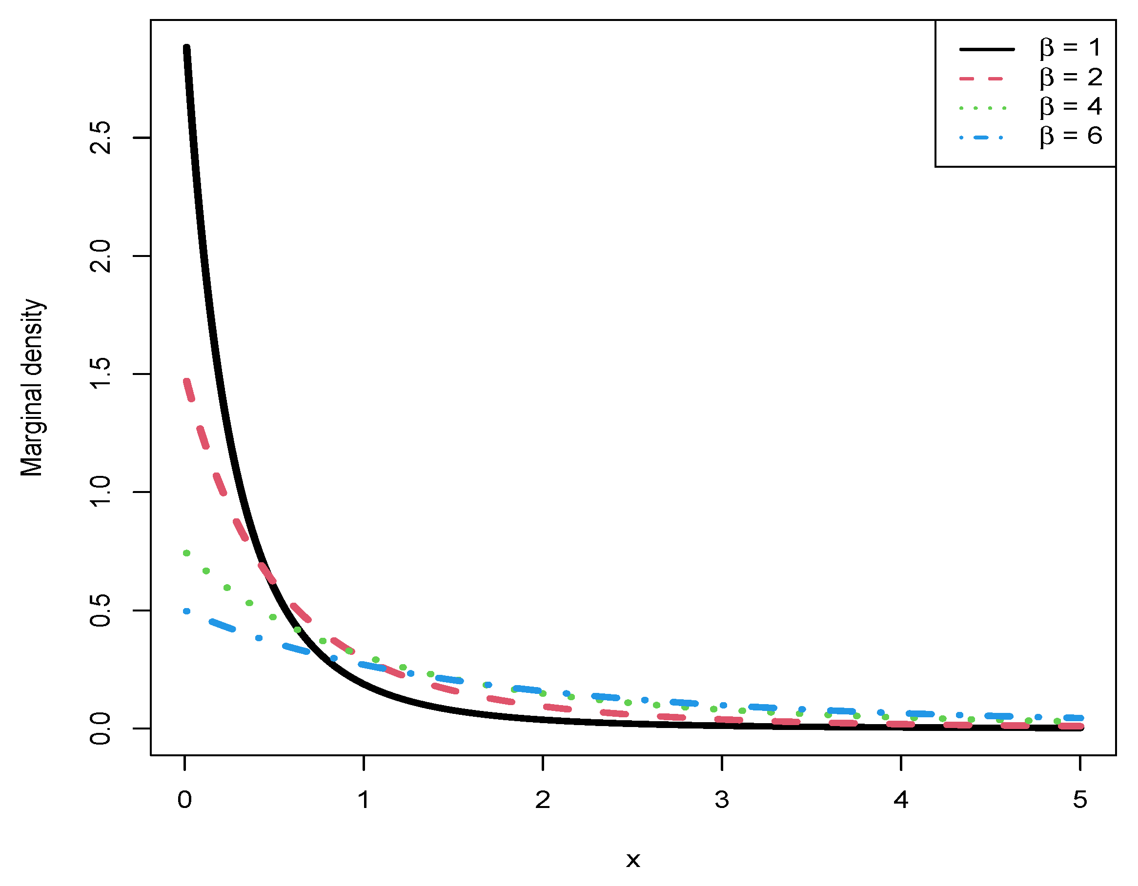
Figure 8 illustrates the marginal densities for different values of
(
), with
kept constant at 3. As observed in the figure, an increase in
corresponds to a reduction in the peak value of the curve. Additionally, all marginal densities exhibit a decreasing trend as functions of
x and display right-skewed distributions.
5. Conclusions and Discussions
The posterior and marginal densities for the exponential-inverse gamma model are calculated in Theorem 1. Subsequently, Bayes estimators as well as PESLs of
are computed. Furthermore, these estimators satisfy two inequalities (
6) and (
7). The hyperparameters of the exponential-inverse gamma model are estimated using the method of moments as embodied in Theorem 2. Additionally, the method of MLE provides estimators for these hyperparameters, which are embodied in Theorem 3. At last, under Stein’s loss, both methods yield empirical Bayes estimators for a mean parameter of an exponential-inverse gamma model as presented in Theorem 4.
In the simulation studies, we systematically investigate five critical dimensions of the proposed framework. Firstly, we rigorously validate the inequality relationships between Bayes estimators (
6) and PESLs (
7) under oracle hyperparameter settings. Secondly, we establish the asymptotic consistency of both moment estimators and MLEs for hyperparameter recovery. Thirdly, the model’s fit to simulated data is quantitatively evaluated using Kolmogorov–Smirnov statistics. Fourthly, comprehensive numerical comparisons of PESLs and Bayes estimators are conducted across three approaches—oracle, moment-based, and MLE-driven methods. Finally, we characterize the model’s behavior by visualizing marginal density variations under distinct hyperparameter configurations.
The methods are illustrated using the Static Fatigue 90% Stress Level data.
Table 5 summarizes hyperparameters’ estimators, model’s goodness-of-fit, empirical Bayes estimators of mean parameter for exponential-inverse gamma model, PESLs, and mean and variance of Static Fatigue 90% Stress Level data obtained through methods of moment and MLE. The exponential-inverse gamma model, when hyperparameters are calculated by the method of MLE, exhibits a superior goodness-of-fit to real data compared to that calculated by the method of moments. Furthermore, we demonstrate (
6) and (
7) for the real data.
The numerical results imply that MLEs outperform moment estimators in calculating hyperparameters and . Nevertheless, this improvement has a cost. In comparison to moment estimators, MLEs require more computational resources, are numerically unstable, necessitate greater than 0 throughout the process of iteration, and lack closed-form answers. Hyperparameters’ MLEs are highly ingenious for starting estimations, whereas estimators from the method of moments often serve as reliable initial estimates. Furthermore, if there are cases where MLEs are virtually nonexistent, the presence of a valid reason allows us to utilize estimators from the method of moments.
The inverse gamma prior was chosen for its conjugacy with the exponential likelihood, ensuring analytical tractability in deriving Bayes estimators and PESL—a critical first step in establishing theoretical properties for this underexplored model. While focusing on a single prior limits generality, it provides a foundational framework for future extensions to broader classes (e.g., non-conjugate or robust priors), which we acknowledge as valuable next steps. Our goal here was to rigorously address the uniqueness of Stein’s loss in this specific hierarchical setting, but we agree that exploring prior sensitivity would enrich the analysis and plan to investigate this in subsequent work.
The exponential model was chosen for its conjugacy with the inverse gamma prior, enabling closed-form derivations of Bayes estimators and PESL under Stein’s loss—a key focus of our theoretical analysis. This simplicity allowed us to rigorously isolate the impact of Stein’s loss in restricted parameter spaces, with direct applications to reliability (e.g., fatigue data). While the exponential case serves as a foundational step, extending this framework to other models (e.g., Weibull, gamma) would broaden its utility. Such extensions, though computationally challenging, are a promising direction for future work, and we appreciate the reviewer’s emphasis on this potential.
While our focus was on the conjugate inverse gamma prior for analytical tractability, the methodology can theoretically accommodate non-conjugate or loss-informed priors. However, this would require numerical methods (e.g., Markov Chain Monte Carlo (MCMC)) for posterior computation and alter the closed-form Bayes estimators and PESL expressions.
Direct numerical comparison with MCMC is challenging due to fundamental methodological differences: MCMC requires hyperpriors to ensure posterior integrability (full Bayesian), while our empirical Bayes approach avoids hyperpriors by estimating hyperparameters from data. However, our method leverages conjugacy to achieve closed-form estimators, eliminating MCMC’s sampling/convergence steps. This yields 10–100× faster computation (e.g., seconds vs. minutes) with comparable accuracy in conjugate settings. While full MCMC excels in generality, our framework prioritizes efficiency for exponential-inverse gamma models.
Stein’s loss was chosen due to its asymmetric penalization of extreme errors (e.g., or ∞), which aligns with our restricted parameter space (). This ensures robustness in reliability contexts (e.g., underestimating failure rates risks catastrophic outcomes). In the supplement, we have highlighted scenarios where Stein’s loss is preferable (positive restricted parameters) versus inappropriate (unrestricted parameters) than the squared error loss function. In this manuscript, the parameter of interest is , the mean parameter of the exponential distribution. Therefore, Stein’s loss function is more appropriate than the squared error loss function. Consequently, we consider the PESL as a criterion to compare Bayes estimators.
The empirical Bayes framework fundamentally differs from full hierarchical Bayesian methods by estimating hyperparameters
via marginal likelihood maximization from observed data (
Section 2.2), rather than assigning hyperpriors. This eliminates hyperprior specification, enhancing computational efficiency and reducing subjectivity—key advantages in conjugate settings like our exponential-inverse gamma model. While empirical Bayes sacrifices full probabilistic coherence, it provides tractable, data-driven estimates ideal for applications requiring rapid inference (e.g., reliability analysis). We emphasize the role of empirical Bayes in balancing computational practicality with robust hyperparameter estimation.


