A Gain Scheduling Approach of Delayed Control with Application to Aircraft Wing in Wind Tunnel

Abstract

The objective of this work is to study the equilibrium stability of a switched linear model with time-delayed control and additive disturbances, that in subsidiary represents the control of wing vibrations in the presence of the turbulence disturbances in an aerodynamic tunnel. The state system is modeled as a collection of subsystems, each corresponding to different levels of air velocity in the wind tunnel. The problem is closely related to the gain scheduling approach for stable control synthesis and to the design of stable, switched systems with time-delay control. A state-predictive feedback method is employed to compensate for actuator delay, resulting in closed-loop free delay switching systems both in presence and absence of disturbances. The main contribution of this study is a thorough analysis of system stability in the presence of disturbances. Finally, numerical simulation results are provided to support and complement the findings.

1. Introduction

This research is motivated by the gain scheduling approach to control synthesis [1], a technique that has been successfully applied to many nonlinear control problems. In flight control, the significant variations in aircraft dynamics across the flight envelope make gain scheduling a particularly effective design strategy. The method involves switching between different controllers based on variations in system parameters, such as aircraft speed or altitude, over time intervals. A novel aspect of this paper is the examination of the gain scheduling technique from the perspective of switched systems. Despite its widespread use, the gain scheduling method lacks sufficient theoretical guarantees regarding the stability and performance of the system to which it is applied, see, for example, [2], making it an ongoing challenge for researchers. This challenge becomes even more complex if time delays in control switches are taken into account, as we address in this paper. In neither of the two sources is the “gain scheduling” problem treated as a “switching system” problem along with all the inherent stability challenges. The same inconsistency is observed in other references available online. Therefore, a novelty of the present article is highlighted.

The basic mathematical problem addressed in this article is to obtain a control law for a switched linear model with time-delayed control and additive disturbances, which guarantees attenuation of the disturbances’ impact on the so-called quality output of the system. To achieve this, a compensator is employed, composed of two components: an observer that estimates the system state based on a measured output, and a static feedback control law based on estimated state prediction, see details at the beginning of Section 3.

Herein, the aim of this study is to present an active control solution to mitigate wing vibrations of a wing in a wind tunnel (WT), which are amplified by the presence of a turbulence generator. In general, the wing and the primary flight control surfaces of an aircraft (the tailplane, the aileron, and the rudder) are flexible structures subject to aeroelastic forces. The interaction among inertial, elastic, and aerodynamic forces can, in extreme cases, lead to a catastrophic aeroelastic phenomenon known as flutter. Even when considering only the inherent structural vibrations, these can be harmful, particularly in terms of structural degradation caused by fatigue.

In recent decades, active vibration control methods have been implemented using the actuators of an aircraft’s primary flight controls or specialized actuators such as piezo or electrical actuators [3,4,5,6]. An alternative approach based on mathematical modelling through experimental identification, combined with active control synthesis validated via numerical simulations, is presented.

This paper is organized as follows. Section 2 introduces the unperturbed model, a linear-switched state model, with constant coefficients and control delay. A solution to the problem is presented, based on the synthesis of a predictive feedback of the state.

Section 3 discusses the switched system model with constant coefficients, control delay, and disturbance.

This work includes both theoretical analysis and experimental validation. The experimental data, used for numerical simulation applications, are provided by the experiment described in Section 4.

Section 5 is dedicated to numerical applications. Numerical simulations are then performed to evaluate the correlation between the system’s behavior and the sufficient stability conditions outlined in the aforementioned theorem.

Section 6 presents the conclusions, summarizing the main findings and contributions of this paper.

2. Linear Mathematical Model Without Disturbances

2.1. Predictive Control Synthesis

Problem 1 (Switching delayed control).

Consider the system

$$\begin{array}{c}\dot{x}\left(t\right)=A_{i}x\left(t\right)+B_{i}u\left(t-h\right),t>0,h>0\\ y(t)=C_{1,i}x(t),z(t)=C_{2,i}x(t),x\left(0\right)=0\\ x(0)=x_0\ne 0,u\left(t-h\right):=u_0\left(t\right),0\le t\le h\\ A_i\in {ℝ}^{n\times n},B_i\in {ℝ}^{n\times 1},C_{1,i}\in {ℝ}^{1\times n},C_{2,i}\in {ℝ}^{1\times n},i=1,\dots ,m\end{array}$$

(1)

where $x\in {ℝ}^{n\times 1}$ is the state; $y(t)$ is the measured output; $z(t)$ is quality output; $u\in ℝ$ is the control; and $h\in {ℝ}_{+}$ is a time delay. Assume that the matrix pairs $\left(A_i,B_i\right)$ and $\left(C_{1,i},A_i\right)$ are at least stabilizable and detectable, respectively [7,8]. Determine the conditions for zero equilibrium stability for $t>0$, given a state feedback control $u\left(\mathit{x}\left(t\right)\right),$initial conditions $u_0\left(0\right)$, $x\left(0\right)$, and a controlled switching law $\mathrm{\sigma }\left(t\right):ℝ\to \left\{1,2,3,\right.\left.4,\dots ,m\right\}$.

The method used to solve the problem is the predictive feedback method [9] which is based on the assumption that the system (1), in the absence of delay, can be stabilized with a feedback control $u\left(t\right)=K_{r,i}x\left(t\right)$. The objective is to find a feedback control law in the presence of the delay such that $u\left(t-h\right)=K_{r,i}x\left(t\right)$, which can be written as $u\left(t\right)=K_{r,i}x\left(t+h\right)$. Although this solution requires future knowledge of the state and may initially seem unimplementable, it is shown in Remark 3 that this is not the case.

Proposition 1.

Consider system (1) with the pairs $\left({\mathit{A}}_i,{\mathit{B}}_i\right)$, $i=1,\dots ,m$, controllable, or at least stabilizable; ${\mathit{A}}_i$ may be even unstable. By introducing the state predictor

$$\begin{array}{c}{x}_p\left(t\right):=x\left(t+h\right)=e^{A_{i}h}x\left(t\right)+{\displaystyle {\int }_t^{t+h}{e}^{A_i(t+h-s)}{B}_{i}u\left(s-h\right)ds}=\\ \equiv e^{A_{i}h}x\left(t\right)+{\displaystyle {\int }_{-h}^0{e}^{-A_{i}s}{B}_{i}u\left(t+s\right)ds}\end{array}$$

(2)

The switching system with control delay (1) can be replaced by the following non-homogeneous closed-loop system with state delay, where $K_{r,i}$ is the gain of the state control law.

$$\begin{array}{c}\dot{x}\left(t\right)=A_{i}x\left(t\right)+A_{d_i}x\left(t-h\right)+B_i{K}_{r,i}{\displaystyle {\int }_{-h}^0{e}^{-A_{i}s}{B}_{i}u\left(t+s-h\right)}ds,\\ u\left(.\right)=K_{r,i}x\left(.\right),A_{d_i}:=B_i{K}_{r,i}{e}^{A_{i}h},t>h.\end{array}$$

(3)

Proof. 

The standard solution for system (1) is given by the following:

$$x\left(t\right)=e^{A_i(t-t_0)}x\left(t_0\right)+{\displaystyle {\int }_{t_0}^t{e}^{A_i(t-s)}{B}_{i}u\left(s-h\right)ds}$$

(4)

With the changes in the integration limits $t_0\to t,t\to t+h,$ it is obtained as follows:

$$x\left(t+h\right)=e^{A_{i}h}x\left(t\right)+{\displaystyle {\int }_t^{t+h}{e}^{A_i(t+h-s)}{B}_{i}u\left(s-h\right)ds}$$

Which is equivalent with (2). Using, for example, the Linear Quadratic Regulator (LQR) algorithm [8], for a pair $\left({\mathit{A}}_i,{\mathit{B}}_i\right)$, a regulator feedback gain $K_{r,i}$ is calculated as if the system was without delay. Introducing the feedback predictive control, as given by the following:

$$u\left(t\right)=K_{r,i}x\left(t+h\right)=K_{r,i}\left(e^{A_{i}h}x\left(t\right)+{\displaystyle {\int }_{-h}^0{e}^{-A_{i}s}{B}_{i}u\left(t+s\right)ds}\right)$$

Which is equivalent to

$$u\left(t-h\right)=K_{r,i}x\left(t\right)=K_{r,i}\left(e^{A_{i}h}x\left(t-h\right)+{\displaystyle {\int }_{-h}^0{e}^{-A_{i}s}{B}_{i}u\left(t+s-h\right)ds}\right)$$

(5)

And substituting this control variable in (1) results in the open-loop system described by Equation (3). □

Corollary 1.

The closed-loop dynamics of the system (1) with the control law (5) is as follows:

$$\begin{array}{c}x\left(t\right)=e^{A_{i}t}x\left(0\right)+{\displaystyle {\int }_0^t{e}^{A_i\left(t-s\right)}}{B}_i{u}_0\left(s\right)ds,\mathrm{if}0\le s\le h,0\le t\le h\\ \dot{x}\left(t\right)=\left(A_i+B_i{K}_{r,i}\right)x\left(t\right),\mathrm{if}t>h\end{array}$$

(6)

Proof. 

Considering Equations (1) and (4) with $t_0=0$ yields the first relation (6), which gives the solution of the dynamical system (1) over the interval $0\le t\le h$. Next, by substituting the control law $u\left(t-h\right)=K_{r,i}x\left(t\right)$ into the dynamical system (1), we obtain the closed-loop dynamical system, the second equation in (6). □

Remark 1.

The regulator feedback gain $K_{r,i}$ is obtained, for example, through a simple linear quadratic regulator (LQR) synthesis [8]. The LQG control synthesis concerns the pairs $\left(A_i,B_i\right),i=1,\dots ,m;$ in the present work $m=4$. Thus, for the system $\dot{x}\left(t\right)=A_{i}x\left(t\right)+B_{i}u\left(t\right)$, the cost functional defined as $J={\displaystyle {\int }_0^{\infty }\left(x^{\mathrm{T}}\left(t\right)Q_{J,i}x\left(t\right)+R_{J,i}{u}^2\left(t\right)\right)}dt$, the feedback control law that minimizes the cost is $u\left(t\right)=K_{r,i}x\left(t\right)$ where $K_{r,i}$ is given by $K_{r,i}=R_J^{-1}{B}_i{P}_i$ and $P_i$ is found by solving the continuous-time algebraic Riccati equation $A_i^{\mathrm{T}}{P}_i+P_i{A}_i-P{B}_i{R}^{-1}{B}_i^{\mathrm{T}}P+Q_{J,i}=0$.

Remark 2.

Consider a fixed index $i,$ $i_0.$ A linear system $\dot{x}\left(t\right)=A_{i_0}x\left(t\right)+B_{i0}u\left(t-h\right)$ with delay is turned into a delay-free system with finite spectrum determined by the roots of the characteristic equation $\det \left(sI-A_{i_0}-B_{i_0}{K}_{r,i_0}\right)=0.$ Through appropriate spectral allocation, each system, activated by the controlled switching law $\mathrm{\sigma }\left(t\right):ℝ\to \left\{1,2\right.\left.,\dots ,m\right\}$, will be stable. The stability of the switched plenary system (1) remains an open question. The first equation in (6) sets the initial conditions for the movement over the interval $\left[0,h\right]$, providing the state $x\left(t\right)$ on this interval and, consequently, the control variable for the next step of integration $\left[h,2h\right]$. The process of controlled movement continues for subsequent steps, in which the system $i_0$ is active, until the switching law triggers the transition to another subsystem indexed with the index $i_1$. The working assumption assumes that switching occurs at integer number of steps of length $h$ and that at the time of switching, the final conditions regarding the state variables associated with system $i_0$ become initial conditions of the states associated with system $i_1$ and so on.

Remark 3.

As stated earlier, we consider that the movement of the switched system (1) begins with the component system with a fixed index $i_0$.The non-homogeneous part of the linear system (3)

$$B_{i_0}{K}_{i_0}{\displaystyle {\int }_{-h}^0{e}^{-A_{i_0}s}{B}_{r,i_0}u\left(t+s-h\right)}ds$$

(7)

is an integral term that naturally contains the effect of state predictor (2). Let us show that the control variable in (3) is causal, meaning that it can be computed at each step based on previous data, in other words, the control law is implementable. During the time interval $\left[0,h\right]$, when no state prediction can yet be applied, the movement of the active system “$i_0$” (herein, there is no state prediction to make, because the first one needs the solution on $\left[0,h\right]$ and then to predict it for $\left[h,2h\right]$!). We start, therefore, with the first step $\left[0,h\right]$ of integration, or of movement, in the physical process. Here, the system (1) with the initial conditions $u_0\left(.\right),$ $x_0,$ has the solution.

$$x\left(t\right)=e^{A_{i_0}\left(t-t_0\right)}{x}_0+{\displaystyle {\int }_{t_0}^t{e}^{A_{i_0}\left(t-s\right)}}{B}_{i_0}{u}_0\left(s\right)ds,0\le s\le h,0\le t\le h$$

(8)

Next, with the solution $x_{i_0}\left(t\right)$ given by (8) on $\left[0,h\right]$, we calculate $u\left(t\right)=K_{r,i_0}{x}_{i_0}\left(t\right)$ and this control variable will be revised by a state prediction, it will modify the system (1) in the system (3) that governs the movement starting with the next step $\left[h,2h\right]$. Therefore, in the following, we are ready to integrate system (3) on the interval $\left[h,2h\right]$, in which $u\left(t\right)=K_{r,i_0}{x}_{i_0}\left(t\right)$ calculated on $\left[0,h\right]$ is already present with the introduced prediction $u\left(t\right)=K_{r,i_0}{x}_{i_0}\left(t+h\right)$; in the discrete integration, the structure of the control “with memory” on the extension of two steps back will be obvious. Let us now check that, on this first step $\left[h,2h\right],$ working with the system (3), the integration is feasible: the control variable varies on Cartesian product $\left[h,2h\right]\times \left[-h,0\right]$ of t and s variation. The left value required for $u$ is $u\left(t+s-h\right)=u\left(h-h-h\right)=u\left(-h\right)$, and the value for the right side of the interval is given by $u\left(t+s-h\right)=u\left(2h-0-h\right)=u\left(h\right)$, meaning that all the values for $u$ are known for the last two steps $\left[-h,0\right]$ and $\left[0,h\right]$. Having the solution $x\left(t\right)$ from the integration on $\left[h,2h\right],$ we are able to perform the integration on $\left[2h,3h\right]$ making $u\left(t\right)=K_{r,i_0}{x}_{i_0}\left(t\right)$ in (3) and so on.

It is simply to verify that the procedure continues in the same manner, providing the state and control values step-by-step. This quasi-detailed description helps clarify the calculations involved, especially from the perspective of an online implementation of the feedback predictive control. This approach to solving the problem with an initial value (1) is known as “the step-by-step method” [10]. The open loop form (3) operates under the conditions of the online process.

2.2. Stability of the Mathematical Model Without Disturbances

The switched delayed linear system (1) is reduced to a system without delay (6). As a result, the problem of system stability is reduced to that of the stability of a switched system

$$\dot{x}\left(t\right)={\mathit{𝒜}}_{\mathrm{\sigma }\left(t\right)}x\left(t\right),x\left(0\right)=0,{\mathit{𝒜}}_{\mathrm{\sigma }\left(t\right)}\in \{{\mathit{𝒜}}_1,\dots ,{\mathit{𝒜}}_m\},{\mathit{𝒜}}_i=A_i+B_i{K}_{r,i}$$

(9)

Both Equation (3), with a visible control variable, and the second equation in (6), with a hidden control variable and without delay, govern in a closed-loop system (1). The first equation describes the system in-process, in-line, while the second describes the closed-loop system off-line. These two equations yield equivalent time histories. The fact that the delay in (3) has been incorporated into the state does not pose any difficulties in numerical simulation. Additionally, it has been shown that the integral inhomogeneous term is causal, allowing it to be computed during the process.

The reason for using the state-predictive control method in this article is that the off-line closed-loop version provides a homogeneous expression (without delay) which has been evaluated in various references with stability theorems. The situation is analogous in the case “with disturbances”. Furthermore, the influence of the delay can be studied in simulations, as it appears as a parameter in the stability conditions [11].

For compliance, we provide the following definition of stability.

Definition 1

([12]). The system (9) is (uniformly) exponentially stable (ES) if there exists a constant $\mathrm{\delta }>0$ such that for all signals $\mathrm{\sigma }$ the solutions of the system (9) with $\left|x\left(0\right)\right|\le \mathrm{\delta }$ satisfy, for some $c,\mathrm{\lambda }>0$, the inequality $\left|x\left(t\right)\right|\le c\left|x\left(0\right)\right|e^{-\mathrm{\lambda }t},\forall t\ge 0$. If the inequality does not depend on the initial condition $\left|x\left(0\right)\right|$, the stability is globally uniformly exponential.

Stability Problem 2

([13]). Determine a minimum dwell time $d^{*}>0$ such that the equilibrium point $\mathit{x}=0$ of the system (9) is exponentially stable with the time switching control $\mathrm{\sigma }\left(t\right)=i\in \{1,\dots ,m\},t\in \left[t_k,t_{k+1}\right)$, where $t_k$ and $t_{k+1}$ are successive switching satisfying $t_{k+1}-t_k\ge d^{*}$ for all $k\in \mathbb{N}$ and the index $i\in \{1,\dots ,m\},$ selected at each instant of $t\ge 0$, is arbitrary. Let us call ${\mathcal{D}}_d$ the set of all switching policies with a dwell time greater or equal to $d$ [14]. Hence, exponential stability is maintained as long as $\mathrm{\sigma }\left(t\right)$ remains unchanged for a period of time greater or equal to the minimum dwell time.

$$d^{*}=\inf \{d\ge 0:(9)\mathrm{is} \mathrm{ES} \mathrm{for} \mathrm{all} \mathrm{\sigma }\left(t\right)\in {\mathcal{D}}_d\}$$

(10)

Theorem 1

([15]). The system (9) is exponentially stable in ${\mathcal{D}}_d$, if and only if there are continuous functions ${\mathcal{V}}_i\left(x\right),i=1,2,\dots ,m$, with properties.

$${\mathcal{V}}_i\left(x\right)>0,\forall x\ne 0,\forall i;\nabla {\mathcal{V}}_i\left(x\right){\mathit{𝒜}}_{i}x<0,\forall x\ne 0,\forall i;{\mathcal{V}}_j\left(e^{{\mathit{𝒜}}_{i}d}x\right)<{\mathcal{V}}_i\left(x\right),\forall x\ne 0,\forall i\ne j$$

(11)

Remark 4.

In relation (11), the functions ${\mathcal{V}}_i\left(x\right),i=1,2,\dots ,m$ will be chosen in the usual simplest form of Lyapunov functions ${\mathcal{V}}_i\left(x\right)=x^{\mathrm{T}}{\mathit{𝒫}}_{i}x,i=1,2,\dots ,m,{\mathit{𝒫}}_i>0,$ symmetrical, as it results as a unique solution from solving the Lyapunov equation ${\mathit{𝒜}}_i^{\mathrm{T}}{\mathit{𝒫}}_i+{\mathit{𝒫}}_i{\mathit{𝒜}}_i=-{𝓠}_i$, for a given ${𝓠}_i>0$.

3. Linear Mathematical Model with Disturbance

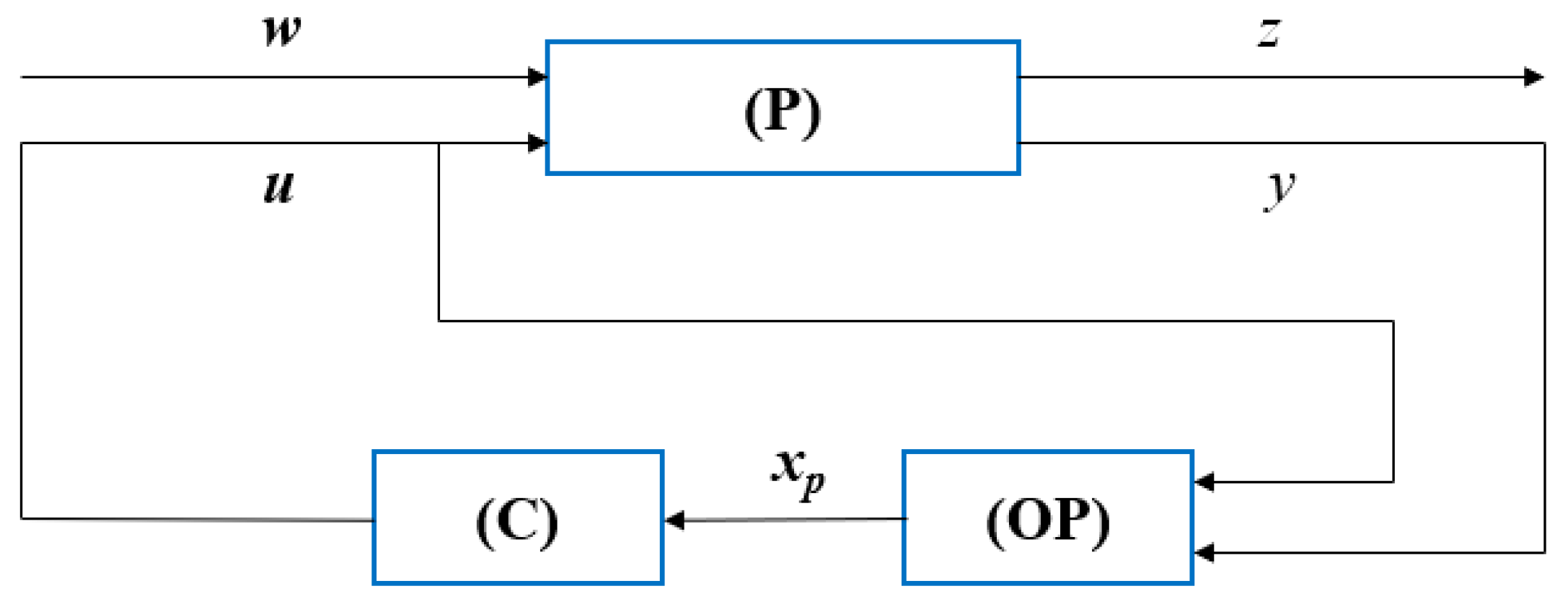
3.1. Using Predictive State Feedback with Observer to Eliminate Control Delay

Consider the switched delayed linear system with disturbance (P) where the variable and matrix sizes are determined according to the application, as will be described in Section 4 and Section 5.

$$\begin{array}{c}\dot{x}\left(t\right)=A_{i}x\left(t\right)+B_{i}u\left(t-h\right)+{\tilde{D}}_{i}w\left(t\right),t\ge 0,h>0,\\ {\tilde{D}}_i:=\left[\begin{array}{cc}{D}_{i,6\times 6}& 0_{6\times 1}\end{array}\right]\in {ℝ}^{6\times 7}\\ y\left(t\right)=C_{1,i}x\left(t\right)+{\tilde{E}}_{i}w\left(t\right),{\tilde{E}}_i:=\left[\begin{array}{cc}{0}_{1\times 6}& E_i\end{array}\right]\in {ℝ}^{1\times 7},\\ z(t)=C_{2,i}x(t),w\left(t\right)=\left[\begin{array}{c}{\xi }_{6\times 1}\\ \mathrm{\eta }\end{array}\right]\in {ℝ}^{7\times 1}\\ x(0)=x_0\ne 0;x(t)=0,\mathrm{if}t<0;w\left(0\right)=w_0=0;\\ u\left(t-h\right):=u_0\left(t\right),\mathrm{if}0\le t\le h\\ A_i\in {ℝ}^{6\times 6},B_i\in {ℝ}^{6\times 1},D_i\in {ℝ}^{6\times 6},C_{1,i}\in {ℝ}^{1\times 6},C_{2,i}\in {ℝ}^{1\times 6}\end{array}$$

(12)

where $x\in {ℝ}^{6\times 1}$ is the state; $u\in ℝ$ is the control; $w\in {\mathcal{L}}_2$ (the space of measurable functions for which the second power of the absolute value is Lebesgue integrable) is a disturbance, inaccessible for measurements; $y\in ℝ$ is the measurement output; $z\in ℝ$ is the quality output; and $h\in {ℝ}_{+}$ is a delay. In all developments in Section 3, it is valid to take the two scalar variables as identical. Suppose that the pairs of matrices $\left(A_i,B_i\right)$ and $\left(C_{1,i},A_i\right)$ are stabilizable and detectable, respectively [8]. The objective is to obtain a control law for the system (12) that guarantees attenuation of the effect of disturbances on the quality output z. For this purpose, a compensator composed of two parts [15] is used: an observer (O), which estimates the state based on the measured output y (therefore, there is no need to know the full state vector x) and a static feedback control law (C), based on observer state prediction. The structure of the observer is as follows:

$${\dot{x}}_o(t)=A_i{x}_o(t)+B_{i}u(t-h)-K_{o,i}(y(t)-C_{1,i}{x}_o(t)),K_{o,i}\in {ℝ}^{6\times 1}(\mathbf{O})$$

(13)

where $x_o(t)$ is the observer state and $K_{o,i}$ is the gain of the observer determined so that the matrix $A_i+K_{o,i}{C}_{1,i}$ is stable. A static feedback control law based on estimated state prediction is given by the following:

$$\begin{array}{c}{x}_p(t)=e^{A_{i}h}{x}_o(t)+{\displaystyle {\int }_{t-h}^t{e}^{A_i(t-\tau )}{B}_{i}u(\tau )}d\tau ={\displaystyle {\int }_{-h}^0{e}^{-A_i\tau }{B}_{i}u(\tau +t)}d\tau \\ u(t)=K_{r,i}{x}_p(t),K_{r,i}\in {ℝ}^{1\times 6}(\mathbf{C})\end{array}$$

(14)

(note that, naturally, Equation (2) is found). The resulting block diagrams from (12)–(14) are depicted in Figure 1. Further, Propositions 2 and 3 will present in detail some ideas from [16], where the results were presented expeditiously, given the space limitations for a conference-type paper. It should be mentioned, however, that, the model studied in [16] does not include switching.

Proposition 2.

The closed-loop transfer matrix of the system (12)–(14), from $w$ to $z,$ is as follows:

$$\begin{array}{c}{T}_{w\mathrm{z},i}(s)=T_{1,i}(s)+e^{-sh}{T}_{2,i}(s)\\ T_{1,i}(s)=C_{2,i}{\left(sI-A_i\right)}^{-1}\left(I-e^{-sh}{e}^{A_{i}h}\right){\tilde{D}}_i\\ T_{2,i}(s)=C_{2,i}{\left[sI-\left(A_i+B_i{K}_{r,i}\right)\right]}^{-1}\left[e^{A_{i}h}{\tilde{D}}_i-B_i{K}_{r,i}{\left(sI-A_i-e^{-A_{i}h}{K}_{o,i}{C}_{1,i}{e}^{A_{i}h}\right)}^{-1}{e}^{A_{i}h}\left({\tilde{D}}_i+K_{o,i}{\tilde{E}}_i\right)\right]\end{array}$$

(15)

Proof. 

The following is a brief summary of the calculation steps. Note

$$\mathbf{\phi }(t):={\displaystyle {\int }_{t-h}^t{e}^{A_i(t-\tau )}{\tilde{D}}_{i}w\left(\tau \right)d\tau }$$

(16)

Define

$$e_o(t):=x(t)-x_o(t),e_p(t):=x(t)-x_p(t-h)$$

(17)

the estimation error and the prediction error. By direct calculation, it results

$$\begin{array}{c}{\dot{e}}_o(t)=(A_i+K_{o,i}{C}_{1,i})e_o(t)+\left({\tilde{D}}_i+K_{o,i}{\tilde{E}}_i\right)w(t)\\ x(t)=e^{A_{i}h}x(t-h)+{\displaystyle {\int }_{t-h}^t{e}^{A_i(t-\tau )}\left[B_{i}u(\tau -h)+{\tilde{D}}_{i}w\left(\tau \right)\right]d\tau }\\ x_p(t-h)=e^{A_{i}h}{x}_o(t-h)+{\displaystyle {\int }_{t-h}^t{e}^{A_i(t-\tau )}{B}_{i}u(\tau -h)d\tau }\end{array}$$

(18)

Hence,

$$e_p(t)=e^{A_{i}h}{e}_o(t-h)+\mathbf{\phi }(t)$$

(19)

Further,

$$\begin{array}{c}{\dot{x}}_p(t)=e^{A_{i}h}{\dot{x}}_o(t)+A_i{\displaystyle {\int }_{t-h}^t{e}^{A_i(t-\tau )}{B}_{i}u(\tau )d\tau }+B_{i}u(t)-e^{A_{i}h}{B}_{i}u(t-h)\\ {\dot{x}}_p(t)=\left(A_i+B_i{K}_{r,i}\right)x_p(t)-e^{A_{i}h}{K}_{o,i}\left(C_{1,i}{e}_o(t)+{\tilde{E}}_{i}w\left(t\right)\right)\end{array}$$

(20)

Then,

$$x(t)=e_p(t)+x_p(t-h),x(t)=e^{A_{i}h}{e}_o(t-h)+\mathbf{\phi }(t)+x_p(t-h)$$

(21)

therefore, by Laplace transform

$$\widehat{x}(s)=\widehat{\mathbf{\phi }}(s)+e^{-sh}\left(e^{A_{i}h}{\widehat{e}}_o(s)+{\widehat{x}}_p(s)\right)$$

(22)

where $\mathbf{\phi }(t)$ is governed by the differential equation

$$\dot{\mathbf{\phi }}(t)=A_i\mathbf{\phi }(t)+{\tilde{D}}_{i}w(t)-e^{A_{i}h}{\tilde{D}}_{i}w(t-\tau )$$

(23)

or, written in the Laplace transform

$$\widehat{\mathbf{\phi }}(s)={\left(sI-A_i\right)}^{-1}\left(I-e^{A_{i}h}{e}^{-sh}\right){\tilde{D}}_{i}w(s).$$

(24)

From (22) and (24) it results in the following:

$$\begin{array}{c}\widehat{z}(s)=C_{2,i}\widehat{x}(s)=C_{2,i}{\left(sI-A_i\right)}^{-1}\left(I-e^{A_{i}h}{e}^{-sh}\right){\tilde{D}}_{i}w(s)+C_{2,i}{e}^{-sh}\left(e^{A_{i}h}{\widehat{e}}_o(s)+{\widehat{x}}_p(s)\right):=\\ :=T_{1,i}(s)w(s)+C_{2,i}{e}^{-sh}\left(e^{A_{i}h}{\widehat{e}}_o(s)+{\widehat{x}}_p(s)\right).\end{array}$$

(25)

From

$$\begin{array}{c}{\widehat{e}}_0\left(s\right)={\left[sI-\left(A_i+K_{o,i}{C}_{1,i}\right)\right]}^{-1}\left[{\tilde{D}}_i+K_{o,i}{\tilde{E}}_i\right]w(s)\\ {\widehat{x}}_p(s)={\left[sI-\left(A_i+B_i{K}_{r,i}\right)\right]}^{-1}\left(-e^{A_{i}h}{K}_{o,i}\right)\left(C_{1,i}{\widehat{e}}_o(s)+{\tilde{E}}_{i}w(s)\right)\end{array}$$

(26)

it is obtained (see (22)) (the multiplication of matrices $e^{A_{i}h}$ and $sI-A_i$ is commutative)

$$\begin{array}{c}{T}_{2,i}(s)=C_{2,i}{\left[sI-\left(A_i+B_i{K}_{r,i}\right)\right]}^{-1}\left[sI-\left(A_i+B_i{K}_{r,i}\right)\right]e^{A_{i}h}\times \\ \times {\left[sI-\left(A_i+K_{o,i}{C}_{1,i}\right)\right]}^{-1}\left[{\tilde{D}}_i+K_{o,i}{\tilde{E}}_i\right]+C_{2,i}{\left[sI-\left(A_i+B_i{K}_{r,i}\right)\right]}^{-1}\times \\ \times \left(-e^{A_{i}h}{K}_{o,i}\right)\left\{C_{1,i}{\left[sI-\left(A_i+K_{o,i}{C}_{1,i}\right)\right]}^{-1}\left[{\tilde{D}}_i+K_{o,i}{\tilde{E}}_i\right]+{\tilde{E}}_i\right\}=\\ =C_{2,i}{\left[sI-\left(A_i+B_i{K}_{r,i}\right)\right]}^{-1}\times {𝓕}_i\end{array}$$

(27)

where ${𝓕}_i$ is obtained through a meticulous yet instructive calculation

$$\begin{array}{c}{𝓕}_i=\left[sI-\left(A_i+B_i{K}_{r,i}\right)\right]e^{A_{i}h}{\left[sI-\left(A_i+K_{o,i}{C}_{1,i}\right)\right]}^{-1}\left[{\tilde{D}}_i+K_{o,i}{\tilde{E}}_i\right]-\\ -e^{A_{i}h}{K}_{o,i}\left\{C_{1,i}{\left[sI-\left(A_i+K_{o,i}{C}_{1,i}\right)\right]}^{-1}\left[{\tilde{D}}_i+K_{o,i}{\tilde{E}}_i\right]+{\tilde{E}}_i\right\}=\\ =\left\{\left[sI-\left(A_i+B_i{K}_{r,i}\right)\right]e^{A_{i}h}-e^{A_{i}h}{K}_{o,i}{C}_{1,i}\right\}{\left[sI-\left(A_i+K_{o,i}{C}_{1,i}\right)\right]}^{-1}\left[{\tilde{D}}_i+K_{o,i}{\tilde{E}}_i\right]-e^{A_{i}h}{K}_{o,i}{\tilde{E}}_i=\\ =\left\{e^{A_{i}h}sI-e^{A_{i}h}{A}_i-e^{A_{i}h}{K}_{o,i}{C}_{1,i}-B_i{K}_{r,i}{e}^{A_{i}h}\right\}{\left[sI-\left(A_i+K_{o,i}{C}_{1,i}\right)\right]}^{-1}\left[{\tilde{D}}_i+K_{o,i}{\tilde{E}}_i\right]-e^{A_{i}h}{K}_{o,i}{\tilde{E}}_i=\\ =e^{A_{i}h}{\left[{\tilde{D}}_i+K_{o,i}{\tilde{E}}_i\right]}^{-1}-B_i{K}_{r,i}{e}^{A_{i}h}{\left[sI-\left(A_i+K_{o,i}{C}_{1,i}\right)\right]}^{-1}\left[{\tilde{D}}_i+K_{o,i}{\tilde{E}}_i\right]-e^{A_{i}h}{K}_{o,i}{\tilde{E}}_i=\\ =\left\{e^{A_{i}h}-B_i{K}_{r,i}{e}^{A_{i}h}{\left[sI-\left(A_i+K_{o,i}{C}_{1,i}\right)\right]}^{-1}\right\}\left[{\tilde{D}}_i+K_{o,i}{\tilde{E}}_i\right]-e^{A_{i}h}{K}_{o,i}{\tilde{E}}_i=\\ =\left[I-B_i{K}_{r,i}{e}^{A_{i}h}{\left(sI-A_i-K_{o,i}{C}_{1,i}\right)}^{-1}{e}^{-A_{i}h}\right]e^{A_{i}h}\left[{\tilde{D}}_i+K_{o,i}{\tilde{E}}_i\right]-e^{A_{i}h}{K}_{o,i}{\tilde{E}}_i=\\ =\left\{I-B_i{K}_{r,i}{\left[e^{-A_{i}h}\left(sI-A_i-K_{o,i}{C}_{1,i}\right)e^{A_{i}h}\right]}^{-1}\right\}{e}^{A_{i}h}\left[{\tilde{D}}_i+K_{o,i}{\tilde{E}}_i\right]-e^{A_{i}h}{K}_{o,i}{\tilde{E}}_i=\\ =\left\{I-B_i{K}_{r,i}{\left[\left(sI-A_i\right)e^{-A_{i}h}{e}^{A_{i}h}-e^{-A_{i}h}{K}_{o,i}{C}_{1,i}{e}^{A_{i}h}\right]}^{-1}\right\}{e}^{A_{i}h}\left[{\tilde{D}}_i+K_{o,i}{\tilde{E}}_i\right]-e^{A_{i}h}{K}_{o,i}{\tilde{E}}_i\\ =\left[I-B_i{K}_{r,i}{\left(sI-A_i-e^{-A_{i}h}{K}_{o,i}{C}_{1,i}{e}^{A_{i}h}\right)}^{-1}\right]e^{A_{i}h}\left({\tilde{D}}_i+K_{o,i}{\tilde{E}}_i\right)-e^{A_{i}h}{K}_{o,i}{\tilde{E}}_i=\\ =e^{A_{i}h}{\tilde{D}}_i-B_i{K}_{r,i}{\left(sI-A_i-e^{-A_{i}h}{K}_{o,i}{C}_{1,i}{e}^{A_{i}h}\right)}^{-1}{e}^{A_{i}h}\left({\tilde{D}}_i+K_{o,i}{\tilde{E}}_i\right)\end{array}$$

The expressions of $T_{1,i}(s)$ and $T_{2,i}(s)$ are thus obtained. □

Proposition 3.

$T_{2,i}(s)$ is the closed-loop transfer matrix of a system without delay on the states $({\Sigma }^{\prime })$ with a dynamic output feedback compensator $({\Sigma }^{″})$

$$\begin{array}{c}\dot{\varsigma }\left(t\right)=A_i\varsigma \left(t\right)+B_{i}u\left(t\right)+e^{A_{i}h}{\tilde{D}}_{i}w\left(t\right)({\Sigma }^{\prime }),u\left(t\right)=K_{r,i}\widehat{\varsigma }\left(t\right)\\ y_1(t)=C_{1,i}{e}^{-A_{i}h}\varsigma \left(t\right)+{\tilde{E}}_{i}w\left(t\right),z_1(t)=C_{2,i}\varsigma \left(t\right))\\ \dot{\widehat{\varsigma }}\left(t\right)=A_i\widehat{\varsigma }\left(t\right)+B_i{K}_{r,i}\widehat{\varsigma }\left(t\right)+e^{A_{i}h}{K}_{o,i}\left(C_{1,i}{e}^{-A_{i}h}\widehat{\varsigma }\left(t\right)-C_{1,i}{e}^{-A_{i}h}\varsigma \left(t\right)+{\tilde{E}}_{i}w\left(t\right)\right) ({\Sigma }^{″})\end{array}$$

(28)

Proof. 

We apply Laplace transform in the first Equation (28)

$$\begin{array}{c}\left(sI-A_i\right)\varsigma (s)=B_i{K}_{r,i}\left(\widehat{\varsigma }\left(s\right)+\varsigma \left(s\right)-\varsigma \left(s\right)\right)+e^{A_{i}h}{\tilde{D}}_{i}w\left(s\right)\\ \varsigma (s)={\left(sI-A_i-B_i{K}_{r,i}\right)}^{-1}\left[B_i{K}_{r,i}\left(\widehat{\varsigma }\left(s\right)-\varsigma \left(s\right)\right)+e^{A_{i}h}{\tilde{D}}_{i}w\left(s\right)\right]\end{array}$$

(29)

The following remains to be shown:

$$\begin{array}{c}{B}_i{K}_{r,i}\left(\widehat{\varsigma }\left(s\right)-\varsigma \left(s\right)\right)+e^{A_{i}h}{\tilde{D}}_{i}w\left(s\right)\equiv \\ \equiv \left[e^{A_{i}h}{\tilde{D}}_i-B_i{K}_{r,i}{\left(sI-A_i-e^{-A_{i}h}{K}_{o,i}{C}_{1,i}{e}^{A_{i}h}\right)}^{-1}{e}^{A_{i}h}\left({\tilde{D}}_i+K_{o,i}{\tilde{E}}_i\right)\right]w\left(s\right)\\ \widehat{\varsigma }\left(s\right)-\varsigma \left(s\right)=-{\left(sI-A_i-e^{-A_{i}h}{K}_{o,i}{C}_{1,i}{e}^{A_{i}h}\right)}^{-1}{e}^{A_{i}h}\left({\tilde{D}}_i+K_{o,i}{\tilde{E}}_i\right)w\left(s\right)\end{array}$$

(30)

From the two Equation (28), it results in the following:

$$\begin{array}{c}\left(sI-A_i\right)\varsigma (s)=B_i{K}_{r,i}\widehat{\varsigma }\left(s\right)+e^{A_{i}h}{\tilde{D}}_{i}w\left(s\right)\\ \left(sI-A_i-e^{A_{i}h}{K}_{o,i}{C}_{1,i}{e}^{-A_{i}h}\right)\widehat{\varsigma }\left(s\right)=B_i{K}_{r,i}\widehat{\varsigma }\left(s\right)-e^{A_{i}h}{K}_{o,i}{C}_{1,i}{e}^{-A_{i}h}\varsigma \left(s\right)-e^{A_{i}h}{K}_{o,i}{\tilde{E}}_{i}w\left(s\right)\end{array}$$

(31)

We eliminate $B_i{K}_{r,i}\widehat{\varsigma }\left(s\right)$ between the two Equations from (31)

$$\begin{array}{c}\left(sI-A_i\right)\varsigma (s)-\left(sI-A_i\right)\widehat{\varsigma }\left(s\right)+e^{A_{i}h}{K}_{o,i}{C}_{1,i}{e}^{-A_{i}h}\widehat{\varsigma }\left(s\right)-e^{A_{i}h}{K}_{o,i}{C}_{1,i}{e}^{-A_{i}h}\varsigma \left(s\right)-\\ -e^{A_{i}h}{\tilde{D}}_{i}w\left(s\right)=+e^{A_{i}h}{K}_{o,i}{\tilde{E}}_{i}w\left(s\right)\\ \left(sI-A_i-e^{A_{i}h}{K}_{o,i}{C}_{1,i}{e}^{-A_{i}h}\right)\left(\varsigma (s)-\widehat{\varsigma }\left(s\right)\right)=\\ =e^{A_{i}h}\left({\tilde{D}}_i+K_{o,i}{\tilde{E}}_i\right)w\left(s\right)\\ \widehat{\varsigma }\left(s\right)-\varsigma (s)=-{\left(sI-A_i-e^{A_{i}h}{K}_{o,i}{C}_{1,i}{e}^{-A_{i}h}\right)}^{-1}{e}^{A_{i}h}\left({\tilde{D}}_i+K_{o,i}{\tilde{E}}_i\right)w\left(s\right)\end{array}$$

(32)

that is, the last relation (30) and thus Proposition 2 is proven. □

Corollary 2.

The closed-loop system (28) has the expression

$$\begin{array}{c}\left[\begin{array}{c}\dot{\varsigma }\left(t\right)\\ \dot{\widehat{\varsigma }}\left(t\right)\end{array}\right]=\left[\begin{array}{cc}{A}_i& B_i{K}_{r,i}\\ -e^{A_{i}h}{K}_{o,i}{C}_{1,i}{e}^{-A_{i}h}& A_i+B_i{K}_{r,i}+e^{A_{i}h}{K}_{o,i}{C}_{1,i}{e}^{-A_{i}h}\end{array}\right]\left[\begin{array}{c}\varsigma \left(t\right)\\ \widehat{\varsigma }\left(t\right)\end{array}\right]+\left[\begin{array}{c}{e}^{A_{i}h}{\tilde{D}}_i\\ e^{A_{i}h}{K}_{o,i}{\tilde{E}}_i\end{array}\right]w(t)\\ {\mathrm{\zeta }}_{cl}:=\left[\begin{array}{c}\varsigma \left(t\right)\\ \widehat{\varsigma }\left(t\right)\end{array}\right]\in {ℝ}^{12\times 1},y_1\left(t\right)=\left[\begin{array}{cc}{C}_{1,i}{e}^{-A_{i}h}& 0_{1\times 6}\end{array}\right]{\mathrm{\zeta }}_{cl}+{\tilde{E}}_{i}w(t),z_1\left(t\right)=\left[\begin{array}{cc}{C}_{2,i}& 0_{1\times 1}\end{array}\right]{\mathrm{\zeta }}_{cl}\end{array}$$

(33)

Proposition 4.

The matrix $T_1(s)$ is the Laplace transform of a finite impulse with support on $\left[0,h\right]$

$$h_1\left(t\right)=\left\{\begin{array}{c}{C}_{2,i}{e}^{A_{i}t}{D}_i,t\in \left[0,h\right]\\ 0,t>h\end{array}\right.$$

(34)

Proof. 

Indeed, if one refers to (15), we have the following:

$${\displaystyle {\int }_0^h{e}^{A_{i}t}{e}^{-sIt}dt={\displaystyle {\int }_0^h{e}^{-\left(sI-A_i\right)t}dt=}}-{\left(sI-A_i\right)}^{-1}\left[e^{-\left(sI-A_i\right)t}\right]\begin{array}{c}h\\ 0\end{array}={\left(sI-A_i\right)}^{-1}\left(I-e^{-sh}{e}^{A_{i}h}\right)$$

(35)

□

Remark 5.

In turn, the matrix $e^{-sh}{T}_2(s)$ is the Laplace transform of an impulse $h_2\left(t\right)$ with support on $\left[h,\infty \right]$ (otherwise, the Laplace transform is obviously not defined) [17,18]. In this situation, if one consider the transfer matrix from $w$ to $z$, $H\left(s\right)$, it is obtained $h\left(t\right)=h_1\left(t\right)+h_2\left(t\right)$, where $h_1\left(t\right),h_2\left(t\right)$ are the generalized functions (impulse responses) with non-overlapping supports, respectively, the impulse response of $T_{1,i}\left(s\right)$, with bounded support $\left[0,h\right)$, and the impulse response of $e^{-sh}{T}_{2,i}(s)$ with support in $\left[h,\infty \right).$ If the matrix $A_i+B_i{K}_{r,i}$ is stable, then ${‖h\left(t\right)‖}_{𝒜}<\infty$ and ${‖h\left(t\right)‖}_{𝒜}$ = ${‖h_1\left(t\right)‖}_{𝒜}$ + ${‖h_2\left(t\right)‖}_{𝒜}$, where $𝒜$ is a commutative Banach (Wiener type) algebra [19].

From the perspective of the stability of the system (12), respectively (33), it results that the contribution of the component $h_1\left(t\right)$ manifests itself only as an initial condition at the point $h_{-}$. Given the structure of the system (12), one with disturbances, the stability considered is of the Bounded-Input-Bounded-Output type (BIBO) [20].

3.2. BIBO Stability of the Mathematical Model with Disturbances

Let system (33) be rewritten in the following form:

$$\begin{array}{c}{\dot{\mathrm{\zeta }}}_{cl}\left(t\right)=A_{cl,i}{\mathrm{\zeta }}_{cl}\left(t\right)+B_{cl,i}w\left(t\right),y_1\left(t\right)=C_{cl,i}{\mathrm{\zeta }}_{cl}\left(t\right)+{\tilde{E}}_{i}w(t),z_1\left(t\right)=D_{cl,i}{\mathrm{\zeta }}_{cl}\left(t\right)\\ C_{cl,i}:=\left[\begin{array}{cc}{C}_{1,i}{e}^{-A_{i}h}& 0\end{array}\right]\in {ℝ}^{1\times 12};D_{cl,i}:=\left[\begin{array}{cc}{C}_{2,i}& 0\end{array}\right]\in {ℝ}^{1\times 12};{\tilde{E}}_i\in {ℝ}^{1\times 7}\\ {\mathrm{\zeta }}_{cl}\left(t\right)=\left[\begin{array}{c}\varsigma \left(t\right)\\ \widehat{\varsigma }\left(t\right)\end{array}\right]\in {ℝ}^{12\times 1},w\left(t\right)=\left[\begin{array}{c}{\xi }_{6\times 1}\\ \mathrm{\eta }\end{array}\right]\in {ℝ}^{7\times 1},{\mathrm{\zeta }}_{cl}\left(0\right)={\mathrm{\zeta }}_{cl,0}\\ A_{cl,i}:=\left[\begin{array}{cc}{A}_i& B_i{K}_{r,i}\\ -e^{A_{i}h}{K}_{o,i}{C}_{1,i}{e}^{-A_{i}h}& A_i+B_i{K}_{r,i}+e^{A_{i}h}{K}_{o,i}{C}_{1,i}{e}^{-A_{i}h}\end{array}\right]\in {ℝ}^{12\times 12};\\ B_{cl,i}:=\left[\begin{array}{c}{e}^{A_{i}h}{\tilde{D}}_i\\ e^{A_{i}h}{K}_{o,i}{\tilde{E}}_i\end{array}\right]\in {ℝ}^{12\times 7}\end{array}$$

(36)

The associated transfer function is ${\mathit{H}}_{cl,i}\left(s\right)=C_{cl,i}{\left(s\mathit{I}-A_{cl,i}\right)}^{-1}{B}_{cl,i}$.

First, the fact that system (36) is a switched one, is ignored, in other words, we consider a fixed $i$. Second, it is assumed that a change in variable has already been performed in (36) to set the nonzero initial state to zero. For such system (36), the condition for BIBO stability is that the impulse response, $h_{cl,i}\left(t\right)$, be absolutely integrable, i.e., its ${\mathcal{L}}_1$ norm exists. It is known that even if each component of a switched system is stable, the stability of the ensemble (in this case, BIBO stability) is not guaranteed. For linear switched systems without disturbances, Theorem 1 provides the nonconservative conditions for exponential stability. The theoretical framework for BIBO stability (so, in the presence of disturbances) of linear switched systems is somewhat more complicated.

The ${\mathcal{H}}_{\infty }$ approach to attenuate the disturbances effect is applied to the switched system (36), with given initial conditions. Recalling the definition of ${\mathcal{D}}_d$ (see Stability Problem 2) and giving a pair of non-negative numbers $\left(d,\gamma \right)$, the aim is to establish conditions to assure that the following applies:

$$J\left(\mathrm{\sigma }\right):=\underset{w\in {\mathcal{L}}_2}{\sup }\left({‖y_1‖}_2^2-{\gamma }^2{‖w‖}_2^2\right)\le 0,\forall \mathrm{\sigma }\in {\mathcal{D}}_d$$

(37)

As noted in [21], it is specified that the optimal control problem with the performance index (37) is practically unsolved. However, with the help of the theorem presented below, it is possible to perform calculations related to the value of the following function:

$$d^{*}\left(\gamma \right)=\underset{d>0}{\inf }\{d:J\left(\mathrm{\sigma }\right)\le 0,\forall \mathrm{\sigma }\in {\mathcal{D}}_d\}$$

(38)

For the statement of the next theorem, the following notations are necessary:

$$\begin{array}{c}{H}_i=A_{cl,i}+B_{cl,i}{\left({\gamma }^2{I}_{7\times 7}-{\tilde{E}}_i^{\mathrm{T}}{\tilde{E}}_i\right)}^{-1}{\left(P_i{B}_{cl,i}+C_{cl,i}^{\mathrm{T}}{\tilde{E}}_i\right)}^{\mathrm{T}}\\ R_i\left(d\right)=P_i-e^{H_i^{\mathrm{T}}d}{P}_i{e}^{H_{i}d},S_i={\displaystyle {\int }_0^{\infty }{e}^{H_{i}t}{B}_{cl,i}}\left(I-{\gamma }^{-2}{\tilde{E}}_i^{\mathrm{T}}{\tilde{E}}_i\right)B_{cl,i}^{\mathrm{T}}{e}^{H_i^{\mathrm{T}}t}\mathrm{d}t\end{array}$$

(39)

$P_i$ is the positive definite stabilizing solution of the algebraic Riccati equation

$$0=A_{cl,i}^{\mathrm{T}}{P}_i+P_i{A}_{cl,i}+C_{cl,i}^{\mathrm{T}}{C}_{cl,i}+\left(P_i{B}_{cl,i}+C_{cl,i}^{\mathrm{T}}{\tilde{E}}_i\right){\left({\gamma }^{2}I-E_i^{\mathrm{T}}{\tilde{E}}_i\right)}^{-1}{\left(P_i{B}_{cl,i}+C_{cl,i}^{\mathrm{T}}{\tilde{E}}_i\right)}^{\mathrm{T}}$$

(40)

Theorem 2

([21]). Let $d>0$ be given and the system (36). Assume that there exists a set of positive definite matrices $Z_i$, $i=1,\dots ,m$ of compatible dimensions as follows:

$$\begin{array}{c}\left[\begin{array}{ccc}{A}_{cl,i}^{\mathrm{T}}{Z}_i+Z_i{A}_{cl,i}& Z_i{B}_{cl,i}& C_{cl,i}^{\mathrm{T}}\\ B_{cl,i}^{\mathrm{T}}{Z}_i& -{\gamma }^2{I}_{7\times 7}& {\tilde{E}}_i^{\mathrm{T}}\\ C_{cl,i}& {\tilde{E}}_i& -I\end{array}\right]<0,i=1,\dots ,m\\ \left[\begin{array}{cc}{e}^{H_i^{\mathrm{T}}d}{Z}_j{e}^{H_{i}d}-Z_i+R_i\left(d\right)& e^{H_i^{\mathrm{T}}d}\left(Z_j-P_i\right)\\ \left(Z_j-P_i\right)e^{H_{i}d}& Z_j-P_i-{\gamma }^2{S}_i^{-1}\end{array}\right]<0,i\ne j\in \left[1,\dots ,m\right]\times \left[1,\dots ,m\right]\end{array}$$

(41)

The following are true: (a) the equilibrium solution ${\mathrm{\zeta }}_{cl}=0$ of the switched linear system (36) is globally asymptotically stable $\forall \mathrm{\sigma }\in {\mathcal{D}}_d$; (b) any trajectory of the switched linear system (36) with zero initial condition satisfies $J\left(\mathrm{\sigma }\right)<0,$ $\forall \mathrm{\sigma }\in {\mathcal{D}}_d$.

In the proof of Theorem 2, in [21], the existence of the solution to the Riccati Equation (40) is guaranteed at the cost of increasing the conservatism of the stability conditions established by that theorem.

Theorem 2 evaluates the stability of the systems (12) and (36) represented by the transfer matrices $T_{2,i}(s)$ given in (15), which characterize Dirac impulses applied on $\left[h,\infty \right)$. We assume that the components $T_{1,i}(s)$ do not affect the stability since they are impulses acting only on $\left[0,h\right)$.

Theorem 2 provides conservative (sufficient) conditions for globally asymptotically stability. In other words, it is possible for system (36) to be stable, even if the conditions in the theorem are not fulfilled. It is important to emphasize that three parameters govern the stability in the context of Theorem 2 (see also (36): $h,d,\gamma$). For a closed-loop system of form (36) but without delay, an essential result from [22,23] and another result from [24] allow the determination of a minimal dwell time $d_{\min }$ and an ${\gamma }_{\min }$ (i.e., an optimal, maximum damping of the disturbance). Since the system (36) is one with delay, we will not be able to benefit from those results; therefore, we will approach the analysis of the results provided by Theorem 2 in a different way, as will be numerically explored in Section 5.

Alternative approaches for analyzing the stability of delayed switched systems have been developed in works such as [25,26,27,28], where neuro-fuzzy techniques were used to control physical systems (e.g., thermal manikin and ABS for aircraft application). Other recent results, highly relevant to the scope of this article, are presented in several papers that are reviewed at the end. For instance, in [29], the control problem of high-order fully actuated nonlinear systems with time-varying delays in the discrete-time domain is investigated. In [30], model predictive control was applied to the co-optimization problem of switched systems under time constraints, with guaranteed recursive feasibility and stability. Additionally, in [31], a simultaneous design of a model predictive control plan and a persistent dwell-time switching signal, utilizing conventional multiple Lyapunov–Krasovskii functional, was proposed for linear-delayed switched systems affected by physical constraints and exogenous disturbance.

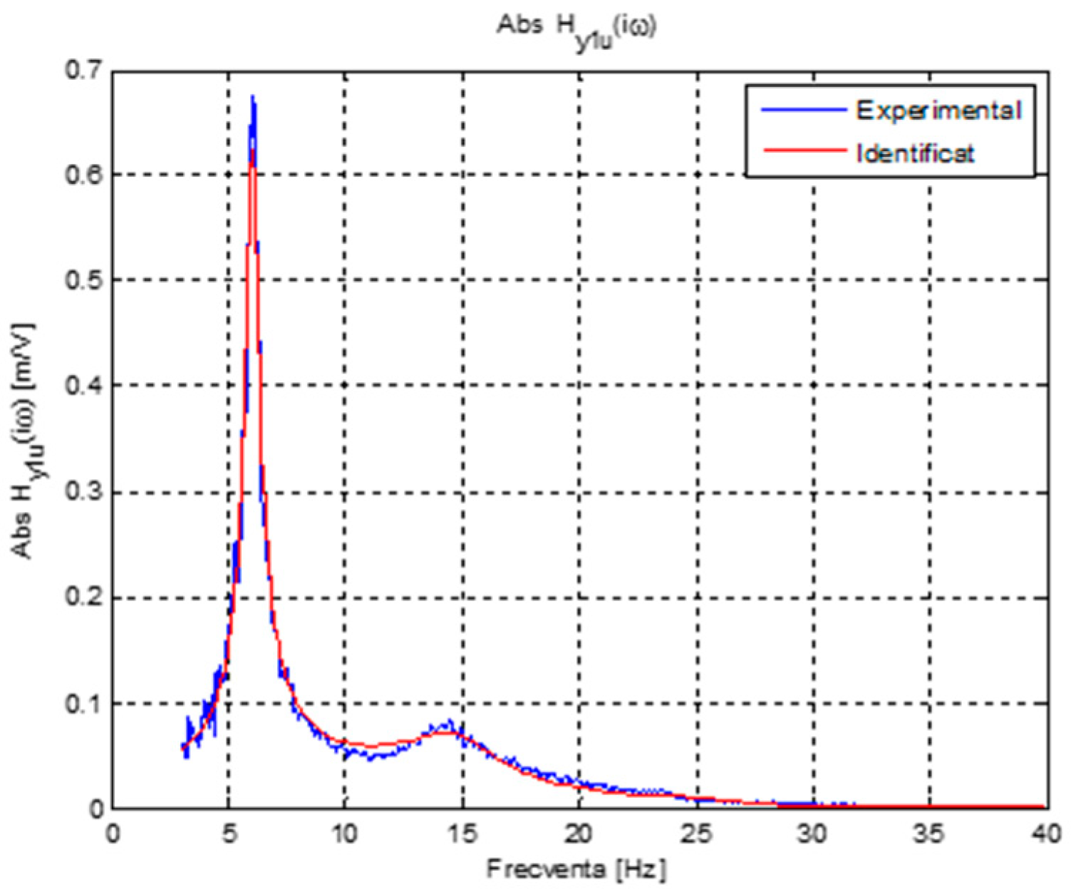
4. Physical Model and Experimental Identification of Mathematical Model

The wing model was specially designed to simulate a realistic, elastic wing, in contrast to the majority of rigid models with external springs simulating basic vibration modes (bending and torsion), as commonly found in the literature [32]. The design condition was to ensure that the uncontrolled system would experience flutter in INCAS subsonic WT [33,34]. The wing structure consists of a longeron covered by an aerodynamic layer, according to the NACA 0012 airfoil profile, Figure 2. One end of the wing features an aileron, while at the other end is a flange that secures the wing in the subsonic WT. The longeron was designed as a rectangular tube with dimensions 1200 × 120 × 25 mm and a thickness of 1 mm. Notches were incorporated to adjust its stiffness. The elements defining the aerodynamic surface were made from wood or resin ROHACELL 71S.

The wing system, consisting of the wing with aileron and piezo actuator, was set-up in the subsonic WT for identification tests at several air speeds (Figure 2) [33,34]. Based on a proof specimen, the flutter speed was determined to be 41 m/s, with a flutter frequency of 5.8 Hz.

The mass (M), damping (C), and stiffness (K) matrices M, C, K (for details, see [35,36,37]) were determined through online identification, since it is much safer than any analytical or FEM approach, given the atypical wing structure. Briefly, the procedure involved identifying the open loop transfer functions $H_{yu}\left(s\right)$ from a chirp signal applied to the piezo actuator. The response was measured by an accelerometer mounted near the wing’s leading edge, capturing both torsional and bending effects. Four air speeds were chosen: V₁ = 15 m/s; V₂ = 20 m/s; V₃ = 25 m/s; V₄ = 30 m/s, accredited as the subsystems $i=1,2,3,4$. The number of poles and zeros corresponding to the four air speeds in WT (see

Table 1. Transfer function $H_{y_{1}u}(i\mathrm{\omega })$ for various air speeds.

Air Speed [m/s]	Poles	Zeros	Frequency ${\mathrm{\omega }}_i$ [Hz]	Damping Ratio  ${\mathrm{\zeta }}_i$
15	−0.9 ± 36.66i	74.93	5.84	0.02
	−3.37 ± 89.69i	−12.52 ± 72.99i	14.30	0.04
	−18.89 ± 1.15i	−43.53	18.61	0.16
20	−1.13 ± 37.19i	294.2	5.92	0.03
	−7.70 ± 95.46i	159.75	15.25	0.08
	−80.95 ± 202.83i	−31.65 ± 51.2i	34.71	0.37
25	−1.34 ± 37.55i	−3064.4	5.98	0.03
	−10.63 ± 94.90i	99.4	15.21	0.11
	−59.80 ± 184.28i	63.4 ± 53.7i	30.83	0.31
30	−1.69 ± 37.73i	1643.3	6.01	0.05
	−13.92 ± 93.95i	−407.6	15.12	0.15
	−81.45 ± 216.13i	126.6; −58.3	36.78	0.35

) were determined using identification procedures in MATLAB/SIMULINK R2019A, ensuring that the frequency responses $H_{yu}\left(i\mathrm{\omega }\right)$ closely matched the experimental data (Figure 3). The experimental transfer functions are very close to those identified when three pairs of conjugate poles were selected, see Table 1. The first two modal frequencies were nearly identical to the measured frequencies 5865 Hz (bending), 14,463 Hz (torsion) of the wing, while the third was close to the presumed frequency of the actuator, 30 Hz. State realizations were obtained for each of the four transfer functions, and further processing was performed to convert the state matrix into the modal form, as follows:

$$\begin{array}{c}{A}_j=\left[\begin{array}{cc}{0}_{3\times 3}& I_3\\ diag\left(-{\mathrm{\omega }}_{j,i}^2\right)& diag\left(-2{\mathrm{\zeta }}_{j,i}{\mathrm{\omega }}_{j,i}\right)\end{array}\right]i=\overline{1,3,}j=1,2,3,4\\ B_1^{\mathrm{T}}=\left[\begin{array}{cccccc}0.17& -0.57& 0.39& 18.80& 54.34& -156.38\end{array}\right]\\ B_2^{\mathrm{T}}=\left[\begin{array}{cccccc}0.26& -1.20& 0.94& 34.90& -43.30& 94.03\end{array}\right]\\ B_3^{\mathrm{T}}=\left[\begin{array}{cccccc}0.24& -0.88& 0.65& 53.78& -100.41& 40.06\end{array}\right]\\ B_4^{\mathrm{T}}=\left[\begin{array}{cccccc}0.28& -0.23& -0.05& 78.63& -176.63& 103.17\end{array}\right].\end{array}$$

(42)

In summary, the mathematical model is obtained through experimental identification using MATLAB subroutines in the frequency domain (see Table 1), in the form of transfer functions, namely rational expressions of polynomials with four zeros (numerator) and six poles (denominator). A MATLAB subroutine is then used to convert the model from the frequency domain to the time domain, yielding the so-called modal form represented by the matrices in (42) for the four air velocities. The corresponding pair for a velocity of 30 m/s is given in (43). Thus, the system defined in (1) is established.

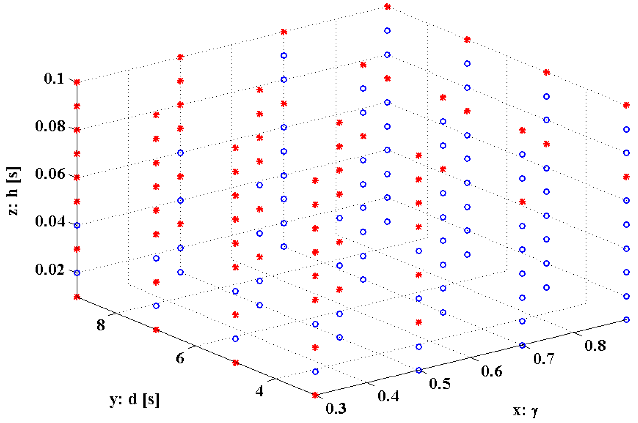
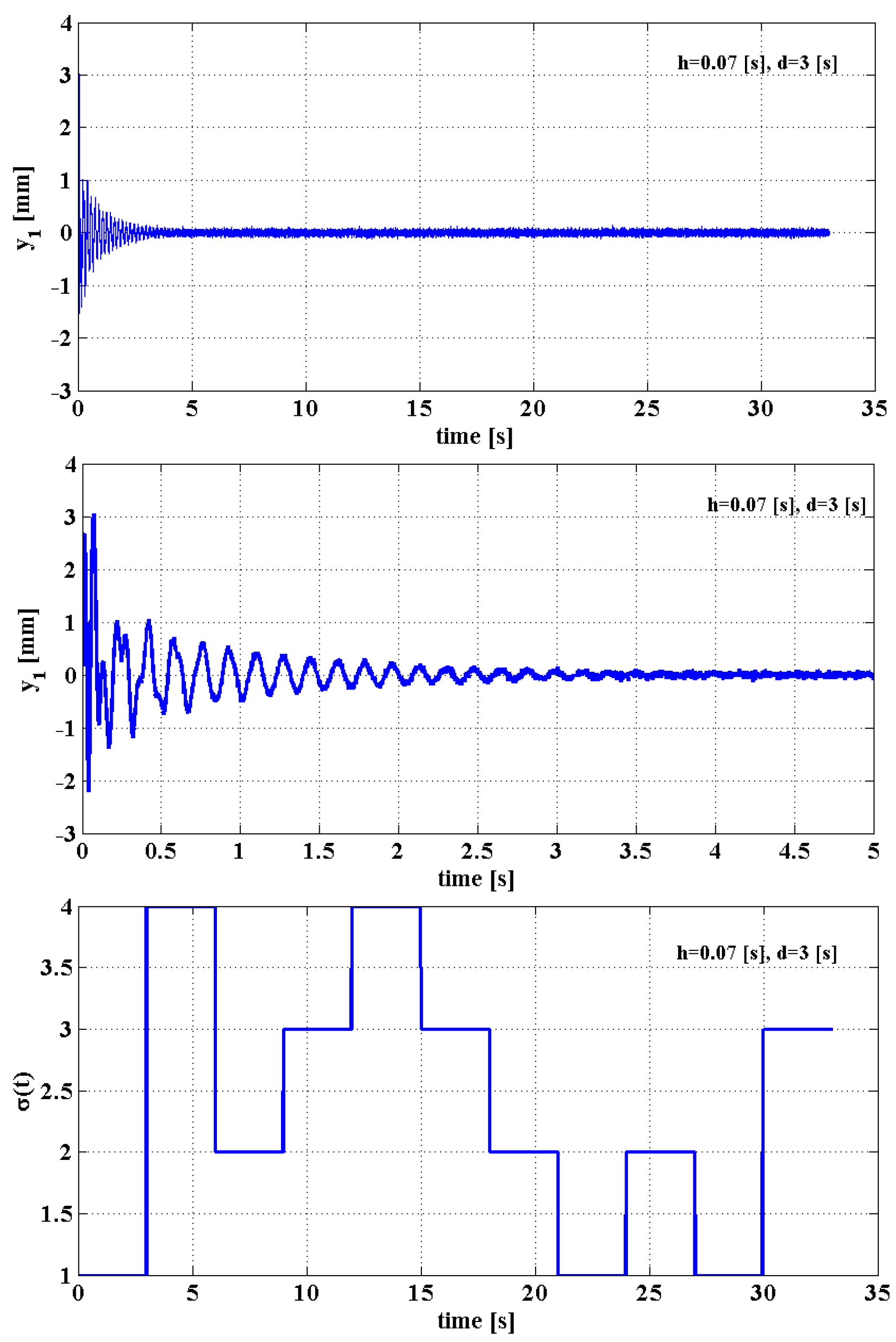
5. Stability Analysis and Numerical Simulations of Wing Model

Starting from the expressions in the frequency domain (see Section 4), the state realizations in time domain were derived. For example, for V₄ = 30 m/s, the identified matrices are as follows:

$$A_4=\left[\begin{array}{cccccc}0& 0& 0& 1& 0& 0\\ 0& 0& 0& 0& 1& 0\\ 0& 0& 0& 0& 0& 1\\ -1427& 0& 0& -3.38& 0& 0\\ 0& -9021& 0& 0& -27.84& 0\\ 0& 0& -\mathrm{53,345}& 0& 0& -162.9\end{array}\right], B_4=\left[\begin{array}{c}0.28\\ -0.23\\ -0.05\\ 78.63\\ -176.63\\ 103.17\end{array}\right]$$

(43)

Four such pairs of matrices constitute the basic elements $A_{cl,i}$, $B_{cl,i}$ for the construction of the system (36). To these are added: $K_{r,i}$—built as an LQR controller [7,8] with $Q_{J,i}$ = diag ([1, 1, 1, 0, 0, 0]); $R_{J,i}$ = 0.1; $K_{o,i}$—built based on a pole placement algorithm $eig\left(K_{o,i}\right)=10\times \left(\mathrm{Re}\left(eig\left(A_i\right)\right)+i\mathrm{Im}\left(eig\left(A_i\right)\right)\right)$; $C_{1,i}$$=\left[1;1;1;0;0;0\right]$=$C_{2,i}$, i = 1, …, 4; ${\xi }_i=\mathrm{\eta }=\mathrm{randn}$ with covariance $1/\sqrt{T,}T=0.001\sec$ (sample time) [38]; $D_{i,6\times 6}$ = diag (0.01); and $E_i$ = 0.001; ${\mathrm{\zeta }}_{cl}\left(0\right)=$$\left[\begin{array}{cccccccccccc}1& 1& 1& 1& 1& 1& 0& 0& 0& 0& 0& 0\end{array}\right]$.

The fact that the delayed system (36) starts at time $t_0=h$ (see [11]), with certain initial values of the variables, was ignored, as it does not affect the stability evaluated by Theorem 2. Clearly, the stability of the delayed switched system depends on the three parameters: $\gamma$ (the amount of damping required for disturbance attenuation); $d-$dwell time (the time of action of the switched system components until switching to another component/the duration for which a switched system component remains active before switching to another component); $h-$time delay on control. For these parameters, several point values were considered, placed along on the three rectangular edges (axes) of a cube originating from the same vertex; thereby defining a “stability cube”, Figure 4: axis $x$, $\gamma =\left(0.3;0.5;0.7;0.9\right)$; axis $y$, $d=\left(3;5;7;9\right)\sec$; axis $z$, $h=\left(0.01;0.02;\dots ;0.1\right)\sec$. For each of the 160 configurations, Theorem 2 produces a decision of either a “stability” (blue circle) or an “instability” (red asterisk).

A set of numerical simulation results is presented below. Since numerical simulation usually works with discretized systems, see [11], as in this work, the interval length $h$ (time delay) is divided into $l$ steps, $T=h/l,T-$sampling time. System (36) is in closed loop; therefore, the control is not explicitly shown, but, at the rigor, the maximum value is taken into account, $u_{\max }=10 V.$ The configuration of subsystems switching was considered: = [1 4 2 3 4 3 2 1 2 1 3], at d second intervals. A white noise $w\left(t\right)=\left[\begin{array}{c}{\xi }_{6\times 1}\\ \mathrm{\eta }\end{array}\right]$ of zero mean and covariance 1 was introduced to simulate turbulence in a simplified manner. It should be mentioned that the lines of the system (6) represent the following states, in order: $x_1-$bending displacement, $x_2-$torsion, $x_3-$actuator state, $x_4-$bending speed, $x_5-$torsion speed, and $x_6-$actuator speed.

The results from the table of configurations $\left(d,h,\gamma \right)$ categorized in Figure 4 as stable, for any sequence of components, or unstable (but not necessarily), are as expected: stability is generally observed for relatively small $h$ and $\gamma$, and sufficiently large $\gamma$.

For reasons of space saving, only three of these configurations were numerically simulated to represent the output $y_1$ as a result. The graphs are given in Figure 5, for the configuration $\left(d=9,h=0.06,\gamma =0.9\right)$, confirmed as stable; in Figure 6, for the configuration $\left(d=3,h=0.07,\gamma =0.7\right)$, disproved as unstable; and in Figure 7, for the configuration $\left(d=3,h=0.15,\gamma =0.9\right)$, confirmed as unstable. In all cases, the same sequence of models was performed: [1 4 2 3 4 3 2 1 2 1 3]. The simulation results revealed that the damping is quantitatively (not qualitatively) influenced by the sequence of models.

6. Conclusions

The main novelty of this article lies in the elaboration of a complex procedure for the active vibration control of an elastic model of a wing with aileron in the presence of turbulence generated in a wind tunnel. A methodology for the experimental identification of the mathematical model is outlined and briefly presented in Section 4. More significantly, the mathematical framework developed in Section 3 was applied to a real-world model, distinguishing this article from typical studies in the literature, where theories are often illustrated using didactic models of 2 × 2 matrices (see, for example, [21]). Thus, it should be noted that applying theory to real-world physical systems can lead to unexpected challenges; however, this was not the case here. Additional novel contributions are outlined below.

The physical–mathematical model studied is closely related to the widely used gain scheduling approach in aircraft control. The mathematical model of the wing, obtained through experimental identification, consists of a set of linear systems corresponding to several air speeds in WT. Introducing actuator delay into the model is a common practice in the field. Thus, this paper defines an active control synthesis problem for a switching system with actuator delay. To compensate for the actuator delay, a state predictive feedback method is applied, resulting in a closed-loop, delay-free switching system. Section 2 serves as a preparation for the main contributions presented in Section 3. Propositions 11 and 12 provide detailed explanations of concepts from [16], where the results were presented expeditiously, due to the space limitations for a conference-type paper. It should be mentioned, however, that, the model in [16] does not include switching. Additionally, the mathematical model present in [16] had to be extended by unifying the state and measure disturbances, in order to be compatible with the ${\mathcal{H}}_{\infty }$ type model in [21]. It is worth mentioning that the mathematical models in [16] are not accompanied by conclusive physical applications.

The equilibrium stability of the closed-loop system (36) is analyzed, in the presence of turbulence disturbances. Numerical simulations highlight some aspects related to the conservative nature of the theorem. It is important to note that the simulations presented here do not provide an exhaustive analysis of all the parameters on which the system depends, due to space constraints. Nevertheless, the results are plausible, particularly in terms of the numerical values of the system states.

References

1. Briat, C. Linear Parameter-Varying and Time-Delay Systems—Analysis, Observation, Filtering & Control; Springer: Heidelberg, Germany, 2015. [Google Scholar]
2. Lin, Z.; Khammash, M. Robust gain-scheduled aircraft longitudinal controller design using an H∞ approach. In Proceedings of the 2001 American Control Conference, Arlington, VA, USA, 25–27 June 2001; Volume 4, pp. 2729–2742. [Google Scholar]
3. Newsom, R.J. Active Control of Aeroelastic Response; TM-83179; NASA: Washington, WA, USA, 1981.
4. Kratochvíl, A.; Valenta, J. Active flutter suppression for light sport aircraft by a control surface split. CEAS Aeronaut. J. 2024, 15, 977–998. [Google Scholar] [CrossRef]
5. Patartics, B.; Lipták, G.; Luspay, T.; Seiler, P.; Takarics, B.; Vanek, B. Application of Structured Robust Synthesis for Flexible Aircraft Flutter Suppression. IEEE Trans. Control. Syst. Technol. 2022, 30, 311. [Google Scholar] [CrossRef]
6. Waitman, S.; Marcos, A. Active flutter suppression: Non-structured and structured H∞ design. IFAC PapersOnLine 2019, 52, 146–151. [Google Scholar] [CrossRef]
7. Kwon, W.H.; Pearson, A.E. Feedback stabilization of linear systems with delayed control. IEEE Trans. Autom. Control 1980, 25, 266–269. [Google Scholar] [CrossRef]
8. Sontag, E.D. Mathematical Control Theory. In Deterministic Finite Dimensional Systems, 2nd ed.; Springer: Berlin/Heidelberg, Germany, 2013. [Google Scholar]
9. Ursu, I.; Enciu, D.; Tecuceanu, G. Equilibrium stability of a nonlinear structural switching system with actuator delay. J. Frankl. Inst. 2020, 357, 3680–3701. [Google Scholar] [CrossRef]
10. Bellman, R.; Cooke, K.L. Differential-Difference Equations; Academic Press: New York, NY, USA, 1963. [Google Scholar]
11. Toader, A.; Ursu, I.; Enciu, D.; Tecuceanu, G. Towards nonconservative conditions for equilibrium stability. Applications to switching systems with control delay. Commun. Nonlinear Sci. 2023, 121, 107188. [Google Scholar] [CrossRef]
12. Liberzon, D. Switching in Systems and Control; Birkhäuser: Boston, MA, USA, 2003. [Google Scholar]
13. Colaneri, P. Dwell time analysis of deterministic and stochastic switched systems. Eur. J. Control 2009, 15, 228–248. [Google Scholar] [CrossRef]
14. Geromel, J.C.; Colaneri, P. Stability and stabilization of continuous-time switched linear systems. SIAM J. Control Optim. 2006, 45, 1915–1930. [Google Scholar] [CrossRef]
15. Chesi, G.; Colaneri, P.; Geromel, J.C.; Middleton, R.; Shorten, R. A Nonconservative LMI Condition for Stability of Switched Systems with Guaranteed Dwell Time. IEEE Trans. Autom. Control 2012, 57, 1297–1302. [Google Scholar] [CrossRef]
16. Di Loreto, M.; Lafay, J.F.; Loiseau, J.J. Disturbance attenuation by dynamic output feedback for input-delay systems. In Proceedings of the 44th IEEE Conference on Decision and Control, and the European Control Conference, Seville, Spain, 12–15 December 2005. [Google Scholar]
17. Hille, E.; Phillips, R.S. Functional Analysis and Semi-Groups; American Mathematical Soc.: Providence, RI, USA, 1957. [Google Scholar]
18. Baker, R.A.; Vakharia, D.I. Input-output stability of linear time-invariant systems. IEEE Trans. Autom. Control 1970, 15, 316–319. [Google Scholar] [CrossRef]
19. Desoer, C.A.; Vidyasagar, M. Feedback Systems: Input-Output Properties; SIAM: Philadelphia, PA, USA, 2009. [Google Scholar]
20. Antsaklis, P.J.; Michel, A.N. Linear Systems; Birkhäuser: Boston, MA, USA, 2006. [Google Scholar]
21. Geromel, J.; Colaneri, P. H∞ and dwell time specifications of continuous-time switched linear systems. IEEE Trans. Autom. Control 2010, 55, 207–212. [Google Scholar] [CrossRef]
22. Margaliot, M.; Hespanha, J.P. Root-mean-square gains of switched linear systems: A variational approach. In Proceedings of the 2007 46th IEEE Conference on Decision and Control, New Orleans, LA, USA, 12–14 December 2007. [Google Scholar] [CrossRef]
23. Hespanha, J.P. Root-mean-square gains of switched linear systems. IEEE Trans. Autom. Control 2003, 48, 2040–2045. [Google Scholar] [CrossRef]
24. Chesi, G.; Colaneri, P. On the Synthesis of Static Output Feedback Controllers for Guaranteed RMS Gain of Switched Systems with Arbitrary Switching. In Proceedings of the 57th Annual Conference of the Society of Instrument and Control Engineers of Japan (SICE), Nara, Japan, 11–14 September 2018. [Google Scholar] [CrossRef]
25. Ursu, I.; Tecuceanu, G.; Toader, A.; Calinoiu, C. Switching neuro-fuzzy control with antisaturating logic. Experimental results for hydrostatic servoactuators. Proc. Rom. Acad. Math. Phys. Tech. Sci. Inf. Sci. 2011, 12, 231–238. [Google Scholar]
26. Toader, A.; Ursu, I. Pilot modeling based on time delay synthesis. Proc. IME G J. Aero. Eng. 2014, 228, 740–754. [Google Scholar] [CrossRef]
27. Ion-Guţă, D.D.; Ursu, I.; Toader, A.; Enciu, D.; Dancă, P.A.; Năstase, I.; Croitoru, C.V.; Bode, F.I.; Sandu, M. Advanced thermal manikin for thermal comfort assessment in vehicles and buildings. Appl. Sci. 2022, 12, 1826. [Google Scholar] [CrossRef]
28. Ursu, I.; Ursu, F. An intelligent ABS control based on fuzzy logic. Aircraft application. In Proceedings of the ICTAMI 2003, International Conference on Theory and Applications of Mathematics and Informatics, Alba Iulia, Romania, 24–25 October 2003; pp. 355–368. [Google Scholar]
29. Liu, G.-P. Predictive Control of High-Order Fully Actuated Nonlinear Systems with Time-Varying Delays. J. Syst. Sci. Complex 2022, 35, 457–470. [Google Scholar] [CrossRef]
30. Zhuang, S.; Gao, H.; Shi, Y. Model Predictive Control of Switched Linear Systems with Persistent Dwell-Time Constraints: Recursive Feasibility and Stability. IEEE Trans. Autom. Control 2023, 68, 7887–7894. [Google Scholar] [CrossRef]
31. Hassan, Y.F.; Zarkani, M.K.H.; Alali, M.J.; Daealhaq, H.; Chaoui, H. Guaranteed H∞ Performance of Switched Systems with State Delays: A Novel Low-Conservative Constrained Model Predictive Control Strategy. Mathematics 2024, 12, 246. [Google Scholar] [CrossRef]
32. Darabseh, T.T.; Tarabulsi, A.; Mourad, A.-H. Active flutter suppression of a two-dimensional wing using quadratic Gaussian optimal control. Int. J. Struct. Stab. Dyn. 2022, 22, 2250157. [Google Scholar] [CrossRef]
33. Ursu, I.; Ion Guta, D.D.; Enciu, D.; Tecuceanu, G.; Radu, A.A. Flight envelope expansion based on active mitigation of flutter via a V-stack piezoelectric actuator. IOP J. Phys. Conf. Ser. 2018, 1106, 012033. [Google Scholar] [CrossRef]
34. Munteanu, F.; Oprean, C.; Stoica, C. INCAS Subsonic Wind Tunnel. INCAS Bull. 2009, 1, 12–14. [Google Scholar]
35. Iorga, L.; Baruh, H.; Ursu, I. H control with µ-analysis of a piezoelectric actuated plate. J. Vib. Control 2009, 15, 1143–1171. [Google Scholar] [CrossRef]
36. Iorga, L.; Baruh, H.; Ursu, I. A review of robust control of piezoelectric smart structures. Trans. ASME Appl. Mech. Rev. 2008, 61, 17–31. [Google Scholar] [CrossRef]
37. Ursu, I.; Tecuceanu, G.; Enciu, D.; Toader, A.; Nastase, I.; Arghir, M.; Calcea, M. A Smart Wing Model: From Design to Testing in a Wind Tunnel with a Turbulence Generator. Aerospace 2024, 11, 493. [Google Scholar] [CrossRef]
38. Jones, P.W.; Smith, P. Stochastic processes. In An Introduction, 3rd ed.; CRC Press: Boca Raton, FL, USA, 2020. [Google Scholar]
Figure 1. Closed loop system in the problem of disturbance attenuation.
Mathematics 13 01614 g001
Figure 2. (Left): piezo actuator on the test bench; (middle): wing on the modal test bench for corroboration with the experimental identification in the wind tunnel of the structural model; (right): wing in the wind tunnel for active control tests.
Mathematics 13 01614 g002
Figure 3. Amplitude-frequency characteristics of the identified and experimental transfer functions, open loop.
Mathematics 13 01614 g003
Figure 4. “Stability cube”, with axes x , y , z : = γ , d , h ; red asterisk—unstable configuration; blue circle—stable configuration.
Mathematics 13 01614 g004
Figure 5. Stable configuration d = 9 , h = 0.06 , γ = 0.9 ; zoom on the first graph.
Mathematics 13 01614 g005
Figure 6. Configuration d = 3 , h = 0.07 , γ = 0.7 , disproved as unstable; zoom on the first graph.
Mathematics 13 01614 g006
Figure 7. Unstable configuration d = 3 , h = 0.15 , γ = 0.9 .
Mathematics 13 01614 g007