Advanced Mathematical Modeling of Hydrogen and Methane Production in a Two-Stage Anaerobic Co-Digestion System

Abstract

This study introduces a novel mathematical model characterizing the anaerobic co-digestion of wheat straw and waste algal biomass for hydrogen and methane production, implemented in a two-stage bioreactor system. Co-digestion can be a tool to increase biogas production utilizing difficult-to-digest organic waste by introducing easily degradable substrates. Two continuous operational regimes, with organic loading rates of 50 g/L and 33 g/L, were employed to generate the experimental datasets for model parameterization and validation, respectively. Parameter identification was achieved through dynamic experimentation, utilizing three distinct optimization algorithms: the deterministic active-set method (A-S) and the metaheuristics–genetic algorithm (GA), coyote optimization algorithm (COA), and marine predator algorithm (MPA). We assessed the predictive capability of the developed mathematical models using an independent dataset. The models demonstrated good agreement with the experimental data across all measured process variables. Notably, the MPA exhibited superior data fitting accuracy, as quantitatively confirmed by the objective function value, compared to GA, COA, and the A-S algorithm.

1. Introduction

Two-stage anaerobic digestion comes as an important scientific discovery in the developed renewable and sustainable energy biotechnologies that ensures organic waste transformation into biohydrogen and biomethane. It simultaneously copes with the threat of energy crisis and waste accumulation [1]. Anaerobic digestion has been suggested as a relatively cost-effective biotechnology for agricultural waste utilization and green energy production [2]. Lignocellulosic substrates are hard to biodegraded, but this obstacle could be surmounted by the addition of more quickly and easily degradable substrates, so co-digestion comes to help. Co-digestion with microalgal biomass has been used in anaerobic digestion processes to increase biogas production, and this process was economically feasible with improved biodegradability [3]. In addition, in the two-stage system, the separate functioning of the hydrolytic-acidogenic stage and the methanogenic stage is realized to remove the drawbacks that exist in operating a single-stage system [1]. The cascade of two bioreactors exhibits increased process stability, favors the processing of substrates with high organic load, and increases biomethane yields. It has the advantage of producing two energy carriers. In the context of renewable energy production and greenhouse gas emission mitigation, the focus of many research works is on the maximization of the amount of biogas produced with a high percent of hydrogen or methane by the anaerobic digestion of waste organic matter [4,5].

The anaerobic digestion processes are commonly modeled by systems of differential and algebraic equations [6,7], including two-stage systems [8,9].

All model parameters have to be adjusted in a way to obtain maximal benefits. Classical optimization algorithms, such as gradient descent and Newton’s method, are foundational techniques for finding optimal solutions. They work by iteratively improving a candidate solution based on the objective function’s gradient or Hessian. As effective for convex problems, they can struggle with non-convexity, local optima, and high dimensionality [10,11].

Active-set optimization algorithms efficiently handle inequality constraints by identifying the “active” constraints that hold with equality at the solution. They iteratively solve equality-constrained subproblems based on a working set of active constraints, adding or removing constraints until optimality is reached [12,13]. These methods are particularly useful for problems with many constraints, as they avoid explicitly handling all of them at each iteration.

Metaheuristic algorithms, a prominent and evolving area within artificial intelligence, represent a sophisticated approach to problem solving. These algorithms transcend traditional heuristic methods, operating at a “meta” or higher level of abstraction [13,14]. This perspective enables them to navigate complex search spaces and find near-optimal solutions, particularly for problems where conventional optimization techniques prove inadequate.

Metaheuristic algorithms can be broadly categorized into three distinct groups [15,16]. Firstly, evolutionary algorithms, which draw inspiration from biological evolution, encompass techniques such as genetic algorithms (GA), genetic programming, differential evolution, evolutionary strategies, evolutionary programming, and harmony search. Secondly, population-based algorithms, which utilize a collective of potential solutions to explore the search space, include methods such as artificial bee colony optimization (ABC), particle swarm optimization (PSO), ant colony optimization (ACO), antlion optimizer (ALO), coyote optimization algorithm (COA), etc. Finally, trajectory-based algorithms, which iteratively refine a single solution through local search, consist of techniques such as tabu search, simulated annealing, and hill climbing.

There are many successful applications of metaheuristic algorithms for various complex problems [15,16,17,18,19]. Among them, GA, as a classic metaheuristic algorithm, and COA and Marine Predator Algorithm (MPA) have attracted attention.

The COA stands out as a relatively recent addition to the population-based metaheuristic family. Inspired by the social dynamics and environmental adaptation of the Canis latrans species, primarily found in North America, COA offers a unique algorithmic structure [20]. It models the hierarchical social organization of coyotes, their dispersal patterns, and their adaptation to changing environmental conditions. This distinct approach contributes a novel perspective to metaheuristic optimization, setting it apart from existing algorithms. Furthermore, COA incorporates innovative mechanisms for balancing exploration, the process of searching diverse regions of the solution space, and exploitation, the process of refining promising solutions within a localized area [20]. This balanced approach is crucial for achieving efficient and effective optimization, allowing COA to potentially outperform traditional methods in specific problem domains.

A new metaheuristic algorithm–Marine Predator Algorithm (MPA)–has been proposed by Faramarzi [21]. Marine predators exhibit sophisticated foraging strategies guided by prey availability and environmental cues. When prey is scarce, they often employ a Lévy flight strategy, characterized by short, frequent movements interspersed with occasional longer jumps, which is effective for searching sparsely distributed resources. Conversely, in areas with abundant prey, they switch to Brownian motion, involving more localized and random movements, which is sufficient for exploiting readily available food sources. Interestingly, predators maintain a consistent balance between these two movement patterns throughout their lives, suggesting an inherent optimization for encountering prey across varying habitat types.

Environmental factors, such as the formation of ocean eddies or the presence of human-made Fish Aggregating Devices (FADs), can significantly influence predator behavior, prompting them to explore new areas with potentially different prey distributions. The effectiveness of specific movement strategies also depends on the relative speed of the predator and prey. For instance, when prey velocity is low, a predator’s best approach is typically Lévy flight, regardless of the prey’s movement pattern. In situations where predator and prey have similar speeds, Brownian motion becomes advantageous for the predator if the prey utilizes Lévy flight. However, the scale of the environment can influence other scenarios at this velocity ratio. Notably, when prey is significantly faster, the optimal strategy for a predator is often to remain stationary, irrespective of the prey’s movement [21].

MPA design offers simplicity, requires few parameters, and is easy to implement [22,23]. Furthermore, excellent memory retention and high calculation accuracy are advantages, also noted in [24,25].

The application of MPA for various problems has proven to be very efficient [26,27,28]. The MPA performance is found to be superior compared to the COA [29], GA, DE, and PSO [30], GWO and PSO [31,32], WCA, GWO, and CS [33], etc.

To the authors’ knowledge, MPA has not yet been applied for parameter identification of bioprocess models, such as models of anaerobic digestion processes. In the application of MPA for parameter identification problems, for example, the MPA models obtained for photovoltaic model parameter identification [34] or Li-ion battery parameter identification [35] showed excellent matching with experimental data.

In this study, motivated by the results presented so far, the MPA is applied for the first time to identify the parameters of a system of nonlinear differential equations describing the process of two-stage co-digestion for hydrogen and methane production.

The paper explores the application of the MPA, alongside the established GA, COA, and S-A, for the specific purpose of model parameter identification within the anaerobic co-digestion process. The primary objective is to determine the optimal values for the model’s parameters, enabling accurate prediction of the process’s behavior.

The aim of the study is the development of a mathematical model of the process of co-digestion of waste wheat straw and algal biomass for hydrogen and methane production, implemented in two stages.

The main contributions of this research are as follows:

(1)

New mathematical models of an anaerobic co-digestion process are developed and validated. To our knowledge, no such models have been published so far, considering the specific substrate utilized in the suggested digestion process.

(2)

The model’s parameters are identified based on the deterministic active-set algorithm and metaheuristic algorithms–GA, COA, and MPA.

(3)

This work marks the first application of the MPA for model parameter identification of a two-stage anaerobic co-digestion system.

(4)

The developed mathematical models, once validated, offer a powerful tool for in-depth process analysis and optimization.

This paper is organized into four sections. Section 2 details the experimental setup and the optimization algorithms used. Section 3 presents and analyzes the numerical results obtained from the application of A-S, GA, COA, and MPA. Section 4 summarizes our findings and suggests opportunities for future investigations.

2. Materials and Methods

2.1. Experimental Study

The cascade system included two bioreactors with working volumes of 3 dm³ and 15 dm³, respectively. Hydrolysis and acidogenesis participate in the first bioreactor (hydrogen bioreactor (BR₁)) for hydrogen generation, while methanogenesis occurs in the second bioreactor (methane-producing bioreactor (BR₂)). The temperature was under automatic control, and it was maintained at 55 ± 1 °C and 35 ± 1 °C, respectively, at the two reactors. A control system maintains the pH at 5.0 ÷ 5.5 for BR₁ and 6.3–7.2 for BR₂.

The substrate for biodegradation represented a mixture consisting of waste wheat straw and algal biomass in a ratio of 80:20 w/w and was involved in the hydrogen and methane production in the two-reactor system. Data were collected at the maximal daily concentration of hydrogen reached (42.5%) at hydraulic retention time–2 days, while the maximal methane concentration was 56% at hydraulic retention time–6 days.

2.2. Mathematical Model of the Two-Stage Anaerobic Digestion Process

The two-step anaerobic digestion for producing H₂ and CH₄ takes place in two different bioreactors. First, fast-growing acid-producing microbes that make H₂ are grown in the hydrogen bioreactor-BR₁. Then, slow-growing bacteria that make CH₄ are grown in the methane bioreactor-BR₂. The process dynamics in the cascade BR₁ and BR₂ are presented, using mass balance, by a set of five ordinary differential equations (ODEs) and two algebraic equations, as follows [9]:

BR₁:

$${\displaystyle \frac{d{S}_1}{dt}}=-Y_1{\displaystyle \frac{{\mu }_{1max}{S}_1}{K_{S_1}+S_1}}{X}_1+D_1\left(S_{1in}-S_1\right)$$

(1)

$${\displaystyle \frac{d{X}_1}{dt}}={\displaystyle \frac{{\mu }_{1max}{S}_1}{K_{S_1}+S_1}}{X}_1-D_1{X}_1$$

(2)

$${\displaystyle \frac{d{Ac}_1}{dt}}=Y_2{\displaystyle \frac{{\mu }_{1max}{S}_1}{K_{S_1}+S_1}}{X}_1-D_1{Ac}_1$$

(3)

$$Q_{H_2}=Y_{H_2}{\displaystyle \frac{{\mu }_{1max}{S}_1}{K_{S_1}+S_1}}{X}_1$$

(4)

BR₂:

$${\displaystyle \frac{d{X}_2}{dt}}={\displaystyle \frac{{\mu }_{2max}{Ac}_2}{K_{S_2}+{Ac}_2}}{X}_2-D_2{X}_2$$

(5)

$${\displaystyle \frac{d{Ac}_2}{dt}}={-Y}_3{\displaystyle \frac{{\mu }_{2max}{Ac}_2}{K_{S_2}+{Ac}_2}}{X}_2+D_2\left({Ac}_1-{Ac}_2\right)$$

(6)

$$Q_{{CH}_4}=Y_{{CH}_4}{\displaystyle \frac{{\mu }_{2max}{Ac}_2}{K_{S_2}+{Ac}_2}}{X}_2$$

(7)

Equations (1)–(4) show how the amount of the substrate concentration ($S_1$), [g/L]; the microbial biomass concentration ($X_1$), [g/L]; and the acetate formation (${Ac}_1$) [g/L] changes in the BR₁. The algebraic Equation (4) describes the hydrogen yield ($Q_{H_2}$) [mL/day/g VS] in the gas phase of BR₁. $S_{1in}$ [g/L] is the concentration of the input substrate. The Monod kinetics is used to describe how fast the hydrogen-making microbes grow. $D_1$ [day⁻¹] is the dilution rate for the first bioreactor, BR₁; ${\mu }_{1max}$ [day⁻¹] and $K_{S_1}$ [g/L] are Monod kinetic coefficients; and $Y_1$, $Y_2$ and $Y_{H_2}$ are yield coefficients [g/g].

Equations (5)–(7) describe how the acetate ${Ac}_1$ (coming from BR₁) is turned into methane by methanogenic microorganisms. The Monod kinetics is also used here for the specific growth rate of the methanogenic biomass. In the model, $X_2$ is the microbial biomass concentration in BR₂ [g/L], ${Ac}_2$ is the acetate concentration in BR₂ [g/L], $Q_{{CH}_4}$ the methane yield [mL/day/g VS], $D_2$ [day⁻¹] the dilution rate for the second bioreactor BR₂, $Y_{{CH}_4}$ and $Y_3$ are yield coefficients, and ${\mu }_{2max}$ are [day⁻¹] and $K_{S_2}$ [g/L] the kinetic coefficients.

For more clarity, all notations of the model parameters are summarized in

Table 1. Mathematical model notations.

Model Variables
$D_1,D_2$	Dilution rates (day−1)
$S_{1in}$	Inlet cellulose concentration in BR1 (g/L)
$S_1$	Substrate concentration (g/L)
$X_1, X_{12}$	Biomass concentrations (g/L)
${{Ac}_1, Ac}_2$	Acetate concentrations (g/L)
$Q_{H_2}$	Hydrogen yield (mL/day/g VS)
$Q_{{CH}_4}$	Methane yield (mL/day/g VS)
Model Parameters
${{\mu }_{1max},\mu }_{2max}$	Monod kinetic coefficients (day−1)
${K_{S_1}, K}_{S_2}$	Saturation coefficients (g/L)
$Y_1, Y_2, Y_3$	Yield coefficients (g/g)
$Y_{H_2}$	Yield coefficient for hydrogen (g/g)
$Y_{{CH}_4}$	Yield coefficient for methane (g/g)

.

2.3. Active-Set Algorithm

The active-set algorithm, as implemented in MATLAB ver. 22a optimization toolbox, is an iterative method designed to solve constrained optimization problems, particularly quadratic programming (QP) and nonlinear programming (NLP) problems with inequality constraints. This algorithm operates on the fundamental principle of identifying and managing the set of active constraints, meaning they are satisfied with equality at the optimal solution [10,36,37].

The algorithm begins with an initial feasible point and iteratively refines a “working set”, a subset of the constraints hypothesized to be active. At each iteration, a subproblem, typically a QP or linearized NLP based on the working set, is solved to determine a search direction. The step length along this direction is carefully chosen to maintain feasibility with respect to all constraints. If an inactive constraint becomes active during this step, it is added to the working set. Conversely, constraints in the working set that are no longer binding or violate optimality conditions, assessed via Lagrange multipliers, may be removed.

The iterative process continues until the Karush–Kuhn–Tucker (KKT) conditions, necessary for optimality, are satisfied to a specified tolerance. These conditions ensure that the gradient of the objective function lies within the cone spanned by the gradients of the active constraints.

In MATLAB ver. 22a, the active-set algorithm is generally classified as a medium-scale method, suitable for problems with a moderate number of variables and constraints. It is recognized for its robustness, particularly in handling certain non-smooth constraints, and its efficiency when a good initial guess is available, enabling warm starts. However, it may be less efficient than large-scale methods such as interior-point for very large problems. Specific implementations, such as mpcActiveSetSolver, might have additional requirements, such as a positive definite Hessian.

2.4. Genetic Algorithm

GAs have proven to be highly successful in tackling numerous optimization challenges [38]. Their robust nature and adaptability have led to their widespread application in various domains [39,40,41].

Briefly, the GA can be described in the following manner.

The GA operates by encoding potential solutions to a problem as ‘chromosomes’ within a defined parameter space. Initially, a random population of these chromosomes is generated, each representing a possible solution.

To evaluate the quality of each chromosome, a fitness function is employed. This function assigns a ‘fitness’ score to each chromosome, reflecting how well it solves the problem. Chromosomes with higher fitness scores represent better solutions.

Subsequently, the chromosomes are ranked based on their fitness scores. This ranking determines the probability of each chromosome being selected for reproduction. Selection methods, such as roulette wheel selection, favor chromosomes with higher fitness, increasing their likelihood of becoming parents for the next generation. The rationale behind this selection process is to create a new population that, on average, exhibits improved fitness compared to the previous one.

Once selected, parent chromosomes undergo genetic operators to generate offspring. Crossover, a key operator, combines genetic material from two parents, creating new chromosomes with potentially better characteristics. The probability of crossover occurring is controlled by the crossover rate. Following crossover, mutation introduces random changes to the offspring’s chromosomes, diversifying the population and preventing premature convergence to local optima. The mutation rate determines the frequency of these random alterations.

The fitness function is then evaluated for the newly generated offspring, assigning fitness scores that reflect their performance. A reinsertion function determines how the offspring are integrated into the existing population, replacing less fit individuals and maintaining population diversity.

This process of selection, crossover, mutation, and reinsertion is repeated for a predetermined number of generations or until a termination criterion is met. The termination criterion could be reaching a specific fitness level, exceeding a maximum number of generations, or achieving a satisfactory level of convergence. This iterative process mimics natural evolution, gradually refining the population and converging towards optimal or near-optimal solutions.

2.5. Coyote Optimization Algorithm

A metaheuristic approach known as the Coyote Optimization Algorithm draws loose inspiration from the social dynamics of coyotes. Key distinctions from natural behavior include the absence of a second alpha coyote and a fixed number (Nc) of coyotes within each of the Np packs. The following is a brief summary of COA, adapted from [20].

The algorithm initializes a population by forming Np packs, with each pack comprising Nc coyotes. Each coyote in the pack embodies a potential solution, having the same dimensionality (D) as the problem’s search space.

The initialization of the coyotes:

$${soc}_{c,j}^{p,0}={lb}_j+{rand}_j\left({ub}_j-{lb}_j\right)$$

(8)

Each of the D dimensions (j = 1 to D) of a coyote’s initial position is randomly assigned a value within the interval of the lower and the upper bounds [${lb}_j$, ${ub}_j$]. This assignment uses a uniform random number, ${rand}_j$∈ [0, 1], to determine the specific value within that range.

The subsequent adaptation of each coyote is [20]:

$${fit}_c^{p,0}=f\left({soc}_c^{p,0} \right)$$

(9)

The algorithm proceeds iteratively, with f denoting the objective function under evaluation. This iterative process continues for each pack until a predetermined stopping criterion is satisfied. Within each iteration:

• For each pack:

  (1)

  Find the alpha-coyote (best solution) ${min}_{c}f\left({soc}_c^{p,0} \right)$

  (2)

  Find the social tendency of the pack cult.

  (3)

  For each coyote, update the possible new candidate’s social value as:

$${new\_soc}_c^{p,0}={soc}_c^{p,0}+r_1{\delta }_1+r_2{\delta }_2$$

(10)

The movement of each coyote is influenced by two weighted factors: the alpha coyote, with a weight of r₁, and the collective behavior of the pack, with a weight of r₂. The direction of this influence is determined by the vectors δ₁ and δ₂. δ₁ is the positional difference between the alpha coyote and a random pack member (soc), while δ₂ is the difference between the pack’s cultural trend (cult) and another random pack member (soc).

Then, calculate,

$$new\_fit=f\left(new\_soc\right)$$

(11)

$$soc\left(t+1\right)=\left\{\begin{array}{c}new\_soc, if new\_fit<fit\\ soc\left(t\right), otherwise\end{array}\right.$$

(12)

• Pack dynamics involve births and deaths.

  ✓

  A newborn pup’s characteristics (soc) are determined by its parents.

  ✓

  The pup survives if the pack contains at least one coyote with lower fitness (worse adaptation); in such cases, the least fit coyote dies.

  ✓

  If multiple coyotes have lower fitness, the oldest among them dies to make space for the pup.

  ✓

  Otherwise, the pup does not survive.

• Migration between packs.

The probability that a coyote is evicted from a pack is [20]:

$$P_e=0.005\left(N_c^2\right)$$

(13)

• The age of the coyotes is updated.

2.6. Marine Predators Algorithm

Following the common practice of population-based metaheuristics, MPA begins by uniformly distributing initial solutions across the search space [21]:

$$Z_0=Z_{min}+rand\left(Z_{max}-Z_{min}\right)$$

(14)

The initial population in the MPA is generated by randomly distributing solutions within the defined search space. $Z_{min}$ and $Z_{max}$ represent the lower and upper bounds of the search space variables, respectively, and rand is a vector of uniformly distributed random numbers between 0 and 1. This ensures that the initial solutions are spread evenly across the potential solution space, allowing for a comprehensive exploration of the problem.

Drawing inspiration from the ‘survival of the fittest’ principle, MPA assumes that the most proficient predators in nature are highly skilled at locating and capturing prey. Consequently, the algorithm identifies the best-performing solution within the initial population, which is then designated as the top predator. This top predator solution forms the basis of a matrix called Elite, which essentially acts as a repository of the current best solutions. The Elite matrix plays a crucial role in guiding the search process, as its arrays store information about the prey’s (i.e., optimal solution’s) positions, enabling the algorithm to effectively track and pursue the target solution [21]:

$$Elite={\left[\begin{array}{ccc}{Z}_{\mathrm{1,1}}^l& \dots & Z_{1,d}^l\\ ⋮& \ddots & ⋮\\ Z_{n,1}^l& \dots & Z_{n,d}^l\end{array}\right]}_{n\times d}$$

(15)

The Elite matrix is constructed by replicating the vector representing the top predator, denoted as $Z^l$, a total of n times. Here, n signifies the number of search agents within the population, and d represents the dimensionality of the search space. It is important to note that both predators and prey are treated as search agents in this algorithm, reflecting the dynamic interaction where, while predators pursue prey, the prey simultaneously seeks its own sustenance.

After each iteration, the Elite matrix is updated. This update occurs if a new, superior predator is identified, replacing the current top predator and ensuring that the Elite matrix consistently reflects the best solutions found thus far.

A corresponding matrix, named Prey, is also maintained, sharing the same dimensions as the Elite matrix. This Prey matrix stores the positions of all search agents (both predators and prey), and predators dynamically adjust their positions based on the information contained within it. Essentially, the initialization step generates the initial Prey matrix, from which the fittest search agent (the top predator) is selected to populate the Elite matrix. The Prey matrix is mathematically represented as follows [21]:

$$Prey={\left[\begin{array}{ccc}{Z}_{1,1}& \dots & Z_{1,d}\\ ⋮& \ddots & ⋮\\ Z_{n,1}& \dots & Z_{n,d}\end{array}\right]}_{n\times d}$$

(16)

The j-th dimension of the i-th prey is defined by $Z_{i,j}$. Notably, the optimization’s performance is directly and significantly influenced by these two matrices.

The MPA employs a dynamic optimization strategy, dividing the search process into three distinct phases. These phases are designed to simulate the interactions between predators and prey throughout their life cycle while simultaneously adapting to varying velocity ratios. Each phase is assigned a specific iteration period, allowing the algorithm to adjust its search strategy based on the prevailing velocity ratio. This phase-based approach is rooted in the natural behaviors of predators and prey, aiming to mimic their movement patterns and interactions as closely as possible. The following mathematical models are used to implement these three phases:

• Phase 1. High Velocity Ratio (Prey Faster than Predator)

This phase models scenarios where the prey exhibits significantly higher movement speeds than the predator [21].

$$Iter<{\displaystyle \frac{1}{3}}{Iter}_{max}$$

$$\overrightarrow{{Step\_size}_i}=\overrightarrow{R_B}⨂\left(\overrightarrow{{Elite}_i}-\overrightarrow{R_B} ⨂\overrightarrow{{Prey}_i}\right), i=1, \dots , n$$

(17)

$$\overrightarrow{{Prey}_i}=\overrightarrow{{Prey}_i}+P\overrightarrow{R} ⨂ \overrightarrow{{Step\_size}_i}$$

(18)

where the vector $\overrightarrow{R_B}$ represents the Brownian motion, $P$ is a constant number ($P=0.5$[21]), and $\overrightarrow{R}$ is a vector of uniform random numbers in [0, 1].

• Phase 2. Unit Velocity Ratio (Predator and Prey Similar Speed)

This phase represents situations where the predator and prey maintain comparable speeds, resulting in a more balanced interaction [21].

$${\displaystyle \frac{1}{3}}{Iter}_{max}<Iter<{\displaystyle \frac{2}{3}}{Iter}_{max}$$

• first half of the population

$$\overrightarrow{{Step\_size}_i}=\overrightarrow{R_L}⨂\left(\overrightarrow{{Elite}_i}-\overrightarrow{R_L} ⨂\overrightarrow{{Prey}_i}\right), i=1, \dots , {\displaystyle \frac{n}{2}}$$

(19)

$$\overrightarrow{{Prey}_i}=\overrightarrow{{Prey}_i}+P\overrightarrow{R} ⨂ \overrightarrow{{Step\_size}_i}$$

(20)

• second half of the population

$$\overrightarrow{{Step\_size}_i}=\overrightarrow{R_B}⨂\left( \overrightarrow{R_B} ⨂\overrightarrow{ { Elite}_i}-\overrightarrow{{Prey}_i}\right), i=1, \dots , n$$

(21)

$$\overrightarrow{{Prey}_i}=\overrightarrow{{Elite}_i}+P{\left(1-{\displaystyle \frac{Iter}{{Iter}_{max}}}\right)}^{2{\displaystyle \frac{Iter}{{Iter}_{max}}}} ⨂ \overrightarrow{{Step\_size}_i}$$

(22)

where the vector $\overrightarrow{R_L}$ represents the Lévy movement.

• Phase 3. Low Velocity Ratio (Predator Faster than Prey)

This phase simulates conditions where the predator possesses a clear speed advantage over the prey [21].

$$Iter>{\displaystyle \frac{2}{3}}{Iter}_{max}$$

$$\overrightarrow{{Step\_size}_i}=\overrightarrow{R_{BL}}⨂\left( \overrightarrow{R_L} ⨂\overrightarrow{ { Elite}_i}-\overrightarrow{{Prey}_i}\right), i=1, \dots , n$$

(23)

$$\overrightarrow{{Prey}_i}=\overrightarrow{{Elite}_i}+P{\left(1-{\displaystyle \frac{Iter}{{Iter}_{max}}}\right)}^{2{\displaystyle \frac{Iter}{{Iter}_{max}}}} ⨂ \overrightarrow{{Step\_size}_i}$$

(24)

Finally, the FAD’s effect is mathematically presented as [14]:

$$\begin{gathered} if r\le FADs \\ \overrightarrow{{Prey}_i}={\overrightarrow{{Prey}_i}+\left(1-{\displaystyle \frac{Iter}{{Iter}_{max}}}\right)}^{2{\displaystyle \frac{Iter}{{Iter}_{max}}}}\left[{\overrightarrow{Z}}_{min}+\overrightarrow{R} ⨂\left({\overrightarrow{Z}}_{max}-{\overrightarrow{Z}}_{min}\right)\right]⨂\overrightarrow{U, } \end{gathered}$$

(25)

$$\begin{gathered} if r>FADs \\ \overrightarrow{{Prey}_i}=\overrightarrow{{Prey}_i}+\left[FADs\left(1-r\right)+r\right]\left(\overrightarrow{{Prey}_{r1}}-\overrightarrow{{Prey}_{r2}}\right) \end{gathered}$$

(26)

3. Results and Discussion

3.1. Experimental Studies

Experimental studies of continuous anaerobic co-digestion of wheat straw and waste algal biomass at mesophilic conditions are performed. The results are presented in

Table 2. Continuous experiments with 50 g/L organic load.

Duration, day	Dilution Rate, day−1	Hydrogen, mL/day/g VS.	Dilution Rate, day−1	Methane, mL/day/g VS.
0	0.5	11.14	0.1	39.45
1	0.5	14.35	0.1	49.58
2	0.5	14.20	0.1	64.25
3	0.5	13.69	0.1	52.00
4	0.5	10.04	0.1	56.23
5	0.5	9.84	0.1	62.86
6	0.5	11.17	0.1	65.99
7	0.5	10.82	0.1	65.36
8	0.5	10.43	0.1	65.14
9	0.5	9.60	0.1	58.33

for 50 g/L (dataset 1, used for identification) and in

Table 3. Continuous experiments with 33 g/L organic load.

Duration, day	Dilution Rate, day−1	Hydrogen, mL/day/g VS.	Dilution Rate, day−1	Methane, mL/day/g VS.
0	0.33	4.00	0.067	6.81
1	0.33	4.91	0.067	3.34
2	0.33	3.06	0.067	32.73
3	0.33	8.65	0.067	38.64
4	0.33	10.20	0.067	38.40
5	0.33	5.57	0.067	38.08
6	0.33	6.38	0.067	38.32
7	0.33	8.69	0.067	37.25
8	0.33	11.33	0.067	31.69
9	0.33	11.00	0.067	37.40

for 33 g/L (dataset 2, used for verification) organic loading rates.

3.2. Mathematical Modeling

3.2.1. Setup of Numerical Experiments

Equations (1)–(7), which include five ODEs and two algebraic equations, define a mathematical model with seven state variables ($X_1$, $S_1$, ${Ac}_1$, $Q_{H_2},$ $X_2$, ${Ac}_2$, $Q_{{CH}_4}$) and nine unknown parameters (${\mu }_{1max},$ $K_{S_1},$ $Y_1$, $Y_2$, $Y_{H_2}, {\mu }_{2max},$ $K_{S_2}$, $Y_3,{ Y}_{{CH}_4}$).

In the optimization process, each individual within the population–whether a chromosome (GA), coyote (COA), marine predator (MPA) or solution in A-S–encodes a possible solution, specifically a vector of unknown model parameters, p = [${\mu }_{1max}$ $K_{S_1}$ $Y_1$ $Y_2$ $Y_{H_2} {\mu }_{2max}$ $K_{S_2}$ $Y_3{ Y}_{{CH}_4}$]. These parameters, used in the model (Equations (1)–(7)), are encoded within predefined ranges (lower bound (lb) ≤ parameter ≤ upper bound (ub)), determined by prior research [9,42,43] and the authors’ knowledge, as follows:

$$\begin{gathered} 0.01 \le {\mu }_{1max}\le 3; 0.01 \le K_{S_1}\le 5; 0.1 \le Y_1\le 50; \\ 0.01 \le Y_2\le 50; 0.01 \le Y_{H_2}\le 50; 0.01 \le {\mu }_{2max}\le 20; \\ 0.01 \le K_{S_2}\le 5; 0.01 \le Y_3\le 5; 0.01 \le Y_{{CH}_4}\le 100. \end{gathered}$$

(27)

The initial solution for A-S is

$$p_0=[0.6 4 10 1 1 0.01 0.2 0.24 50].$$

Each initial solution for the two metaheuristic algorithms has been generated based on

$$x_j=lb+rand\left(ub-lb\right)$$

(28)

To enhance the solution, algorithms based on natural behaviors (GA, COA, and MPA) were employed to create new solutions, ensuring they adhered to the defined model parameter boundaries. All improved solutions were subsequently checked for compliance.

To maximize the effectiveness of GA, COA, and MPA, their parameters must be precisely tuned to the specific problem. Building upon established parameter ranges found in prior research–GA [44,45,46], COA [47,48,49], and MPA [50,51,52]–and considering the unique characteristics of this model identification problem, an iterative trial-and-error approach was employed. This involved conducting several pretests to refine the parameter settings for each algorithm. To ensure convergence without excessive computational cost, all four algorithms were executed for 100 iterations, a value determined through preliminary testing to be sufficient.

After extensive tuning, the resulting optimal main parameter values for each algorithm are summarized as follows:

GA parameters
population size n	100
generation gap	0.97
crossover rate	0.85
mutation rate	0.1
COA parameters
number of packs Np	50
number of coyotes Nc	100
probability of eviction   of a coyote leave.	0.0005 × Nc2
scatter probability Ps	1/D
association probability Pa	(1 − Ps)/2
MPA parameters
number of predators	100
P	0.5
FADs	0.1

For the GA, specific functions were implemented: a linear ranking fitness function to evaluate solution quality, roulette wheel selection for parent selection, double-point crossover for generating offspring, and bit inversion for mutation. A binary chromosome representation, providing a precision of 20 bits, was chosen to encode the solution space. This binary representation allows for a fine-grained exploration of the parameter space, which is critical for achieving accurate model identification. This meticulous parameter tuning, guided by both existing literature and empirical testing, aimed to maximize the efficiency and effectiveness of each algorithm in solving the target problem.

To facilitate a fair comparison, the stochastic metaheuristics were subjected to 30 runs of 100 iterations, with initial solutions derived from Equation (28) and parameter constraints (lb and ub) applied as defined by Equation (27).

The nine model parameters (p = [${\mu }_{1max}$ $K_{S_1}$ $Y_1$ $Y_2$ $Y_{H_2} {\mu }_{2max}$ $K_{S_2}$ $Y_3{ Y}_{{CH}_4}$]) (search space dimension D = 9) for the system, defined by Equations (1)–(7), were estimated by minimizing the objective function J.

$$\begin{gathered} J=J_{H_2}+J_{{CH}_4}\to min \\ {J}_{H_2}=\sum _{i=1}^n{\left\{\left[{H_2}_{exp}\left(i\right)-{H_2}_{mod}\left(i\right)\right]\right\}}^2 \\ {J}_{{CH}_4}=\sum _{i=1}^m{\left\{\left[{{CH}_4}_{exp}\left(i\right)-{{CH}_4}_{mod}\left(i\right)\right]\right\}}^2 \end{gathered}$$

(29)

where n and m are the lengths of the data vectors for the state variable, $H_2$ and ${CH}_4$ ${H_2}_{exp}$ and ${{CH}_4}_{exp}$ are known experimental data, ${H_2}_{mod}$ and ${{CH}_4}_{mod}$ are model predictions with a given set of parameters.

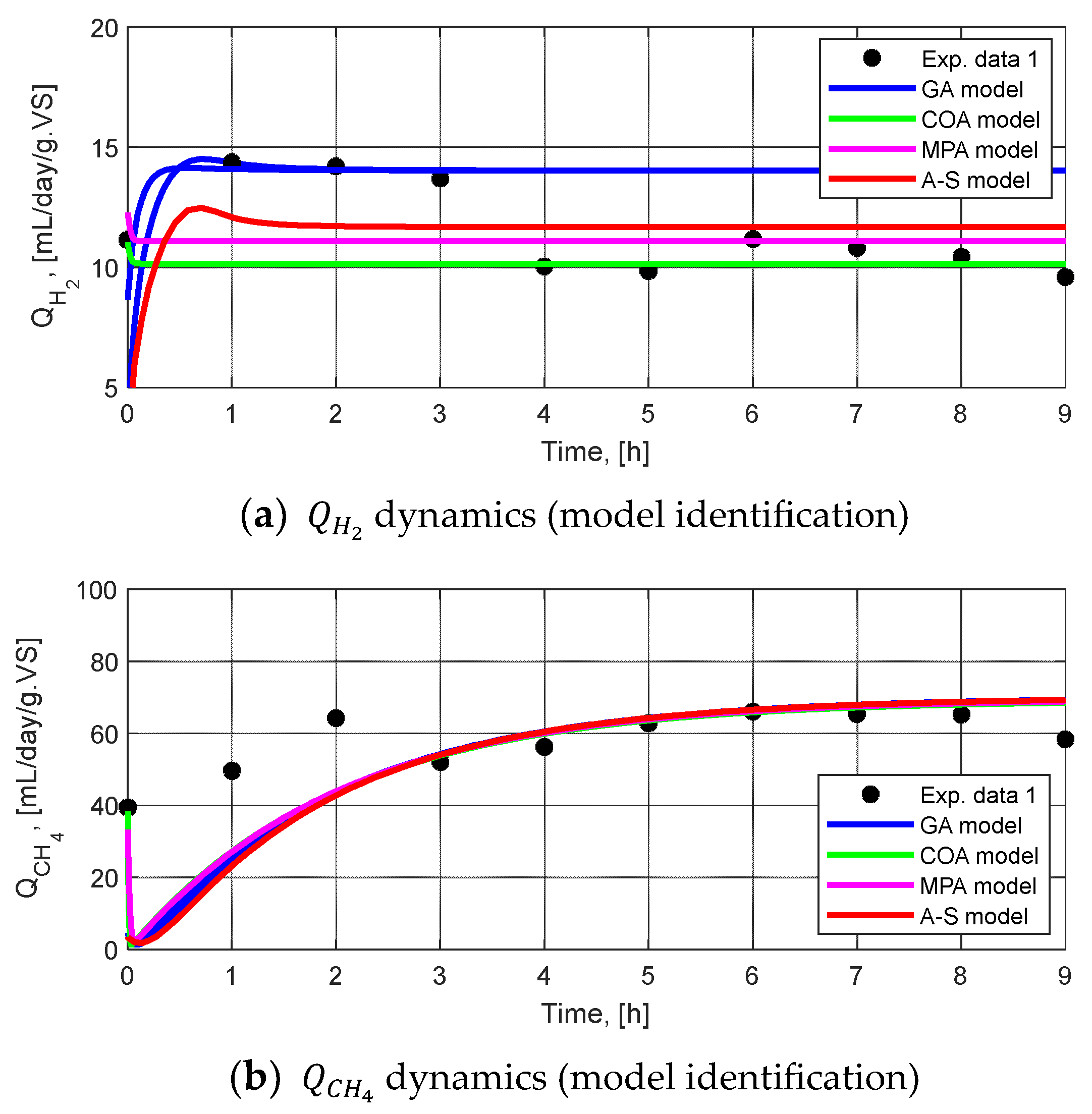
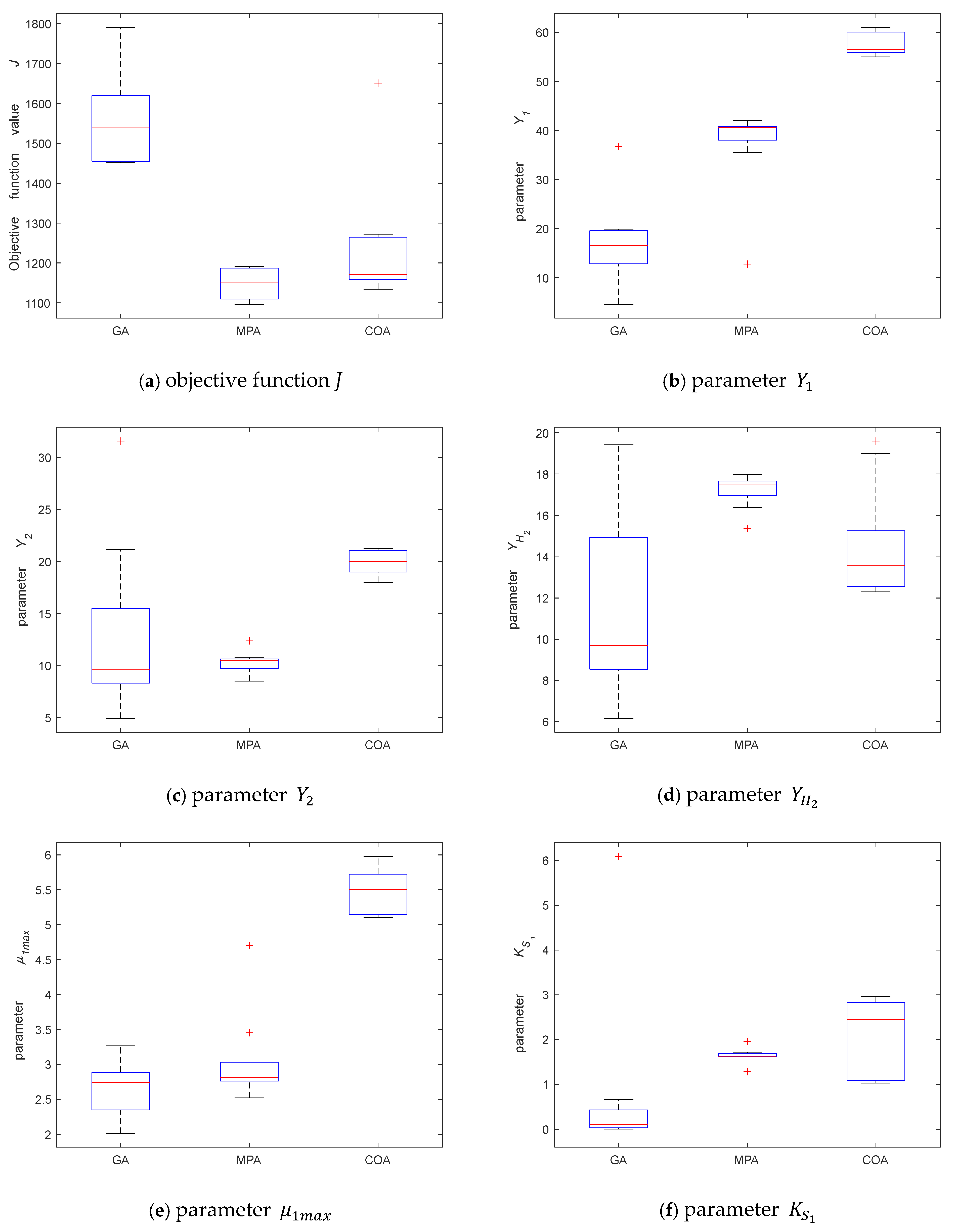
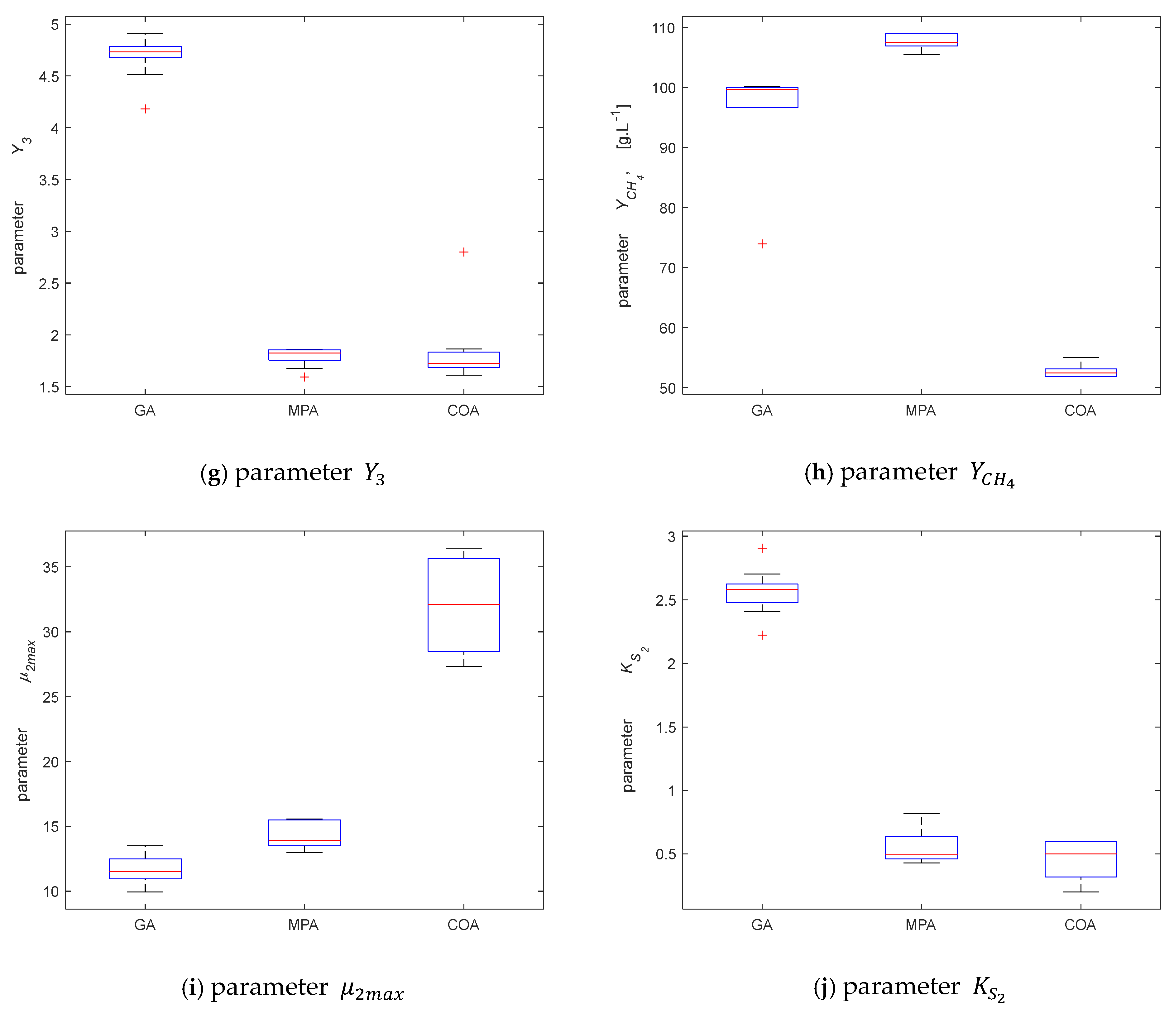
3.2.2. Parameter Identification

To accurately determine the optimal parameters for the proposed mathematical model described by Equations (1)–(7), a comprehensive series of parameter identification procedures was executed. This involved utilizing three distinct metaheuristic algorithms: GA, COA, and MPA, and the A-S algorithm. Before their application, each algorithm was subject to parameter tuning to ensure optimal performance within the specific constraints of the model.

Recognizing the inherent stochastic nature of these algorithms, which introduces variability in their results across different runs, a rigorous statistical approach was adopted. To obtain statistically significant and reliable results, each metaheuristic algorithm was executed 30 independent times.

The best model parameter estimations obtained from these 30 runs for each algorithm are summarized in

Table 4. Model parameter estimations.

Algorithm	Model Parameters
	${\mathit{\mu }}_{1\mathit{m}\mathit{a}\mathit{x}}$	${\mathit{K}}_{{\mathit{S}}_1}$	${\mathit{Y}}_1$	${\mathit{Y}}_2$	${\mathit{Y}}_{{\mathit{H}}_2}$	${\mathit{\mu }}_{2\mathit{m}\mathit{a}\mathit{x}}$	${\mathit{K}}_{{\mathit{S}}_2}$	${\mathit{Y}}_3$	${\mathit{Y}}_{\mathit{C}{\mathit{H}}_4}$
A-S	3.00	3.55	14.16	5.52	6.70	5.03	1.59	3.02	110.00
GA	2.81	4.56	19.92	13.50	11.41	11.89	2.59	4.73	99.66
COA	5.10	2.95	36.66	18.14	14.95	35.56	0.47	1.86	52.43
MPA	2.89	1.61	40.06	9.70	17.88	15.57	0.50	1.88	108.92

. The corresponding objective function values are presented in

Table 5. Objective function values (model identification).

Algorithm	Objective Function	Value	Rank	Total Rank
A-S	$J_{H_2}$	103.13	4	16
	$J_{{CH}_4}$	2614.09	4
	$J$	2717.22	4
GA	$J_{H_2}$	90.87	3	9
	$J_{{CH}_4}$	2360.93	3
	$J$	1451.80	3
COA	$J_{H_2}$	33.76	1	5
	$J_{{CH}_4}$	1100.44	2
	$J$	1134.20	2
MPA	$J_{H_2}$	48.83	2	4
	$J_{{CH}_4}$	1050.10	1
	$J$	1098.93	1

. The objective function values serve as a measure of the model’s fit to the data, with lower values indicating a better fit. Table 3 and Table 4 not only present the optimal parameter values but also provide insight into the performance of each algorithm in terms of solution quality and consistency. The algorithms were ranked according to their performance results.

According to the observed objective function value, the best-performing algorithm is MPA, followed by COA. The worst results were obtained by the A-S algorithm. Due to the novelty of the proposed model of the considered anaerobic process and the absence of established parameter values from prior studies, a definitive quantitative comparison of model performance is challenging. Consequently, it is not possible to rank the algorithms directly or declare a single “best” model based solely on numerical parameter values. Instead, we employed a graphical comparison to evaluate how well the model represented the experimental data visually. This approach allows the identification of systematic deviations, or lack thereof, between the model’s predicted state variables and the actual experimental data.

In Figure 1, the predicted state variables, $Q_{H_2}$ and $Q_{{CH}_4}$, derived from the parameter sets estimated by S-A, GA, COA, and MPA, were plotted alongside the experimental data set 1 from the two-stage anaerobic digestion process. This visual comparison allows for a direct assessment of how well each algorithm’s parameter estimations enable the model to predict the observed experimental process behavior. By examining the graphical representations, we can determine the extent to which the model captures the trends and patterns present in the experimental data, thereby providing a robust qualitative evaluation of the model’s performance.

The four obtained models show similar behavior for methane dynamics. A different behavior was observed in the case of hydrogen dynamics. The experimental data are raw and difficult to predict. The lowest objective function values are obtained by COA and MPA. These algorithms manage to find a solution that is much closer to the experimental data than the other two algorithms–GA and A-S. However, all models predict constant hydrogen concentrations after the first hour of the process, which is not so good.

For a given problem, let O(f(D)) be the computational complexity of its fitness function evaluation. The GA complexity is O(Max_iter × n × f(D)), and the MPA is O(n × f(D) × Max_iter) [22,53], where n is the population size, D is the problem dimension, and Max_iter is the number of iterations. According to [54] the COA complexity is O(n × Max_iter × f(D)). So, the computational complexity of the competing metaheuristic algorithms is identical.

Figure 2 displays box plots illustrating the statistical analysis of the numerical results. This analysis was conducted on data from 30 independent runs of the three stochastic algorithms: GA, COA, and MPA. The box plots visualize key statistical measures for both the estimated model parameters and the resulting objective function value J, including the mean, standard deviation (SD), and median.

The presented box plots show that the MPA statistically performs better than the GA and COA.

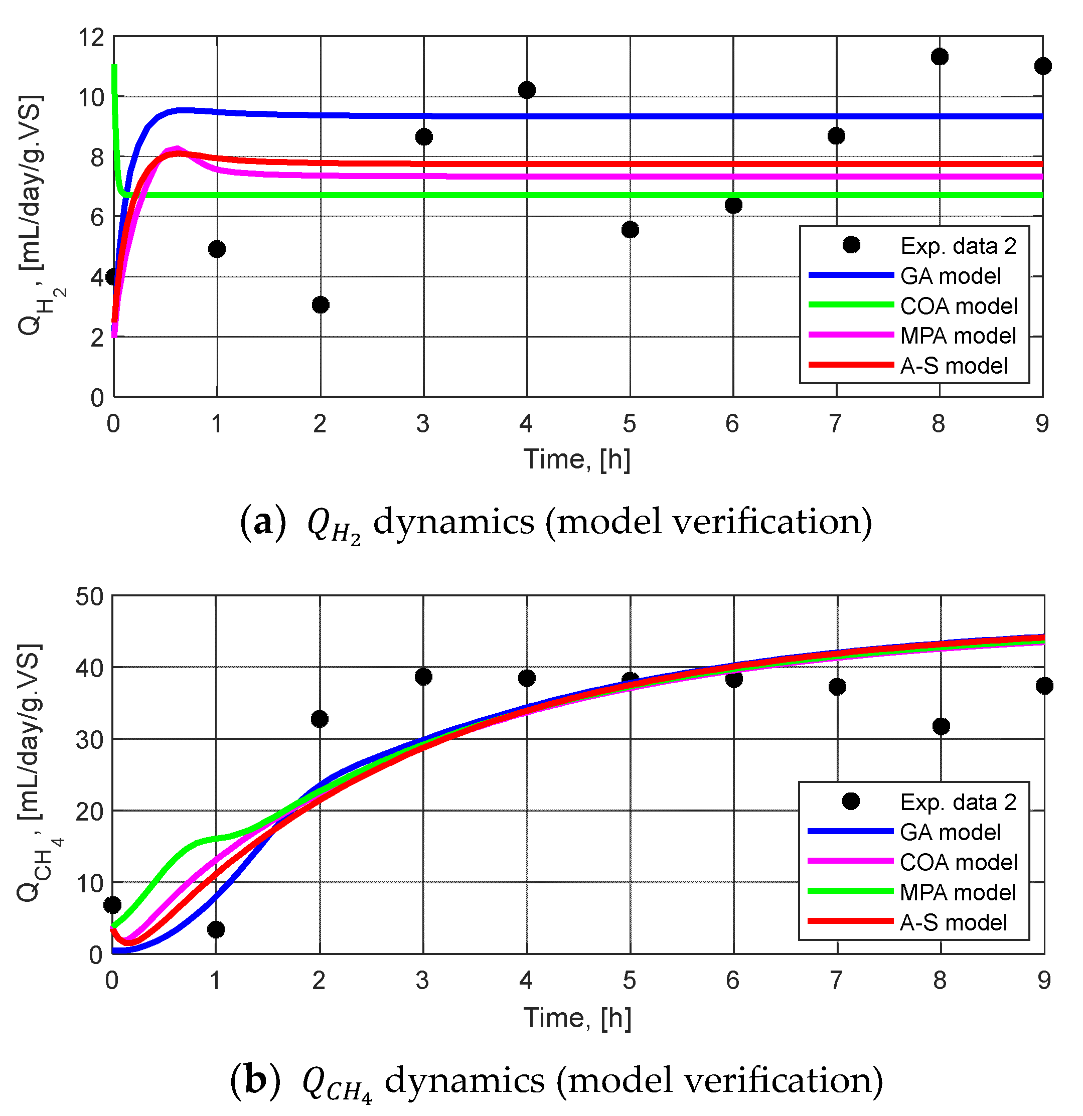
3.2.3. Model Validation

The proposed models are further verified using the experimental data set 2.

Model validation is a crucial process in the development of any model. In essence, it is about evaluating how well a model represents the real-world system it is intended to describe or predict. Model validation helps us determine how much confidence we can have in a model’s outputs and predictions. A well-validated model is more likely to be reliable and useful for decision-making. In our case, the technique for validation includes cross-validation with a different dataset and comparing model outputs to the observations. This information is essential for improving the model, understanding its applicability, and avoiding potential pitfalls in its use.

The four models obtained by GA, COA, MPA, and A-S are validated on the second experimental dataset. The obtained results are presented in

Table 6. Objective function values (model verification).

Algorithm	Objective Function	Value	Rank	Total Rank
A-S	$J_{H_2}$	71.56	1	8
	$J_{{CH}_4}$	519.85	4
	$J$	591.41	3
GA	$J_{H_2}$	96.11	3	6
	$J_{{CH}_4}$	449.39	2
	$J$	545.50	1
COA	$J_{H_2}$	137.57	4	11
	$J_{{CH}_4}$	486.71	3
	$J$	624.28	4
MPA	$J_{H_2}$	83.42	2	5
	$J_{{CH}_4}$	499.25	1
	$J$	582.67	2

. The observed error values (calculated by applying Equation (28)) for each of the developed mathematical models are compared and ranked.

The results in Table 6 show that, again, the best results are observed by the MPA mathematical model. The COA model does not predict the real data very well. Although the model was second-best, on the verification stage, the model failed. The GA model shows similar behavior to MPA when the model is compared to the second set of real data.

The comparison of the model predictions and the real data (experimental dataset 2) is presented in Figure 3.

Based on the presented results, the mathematical model obtained by MPA shows the best performance compared to the other three algorithms. To improve the model, more sets of experimental data are needed. The carrying out of a series of new experimental digestion processes will be one of the further work directions.

For describing various anaerobic fermentation processes, many mathematical models have been suggested [55]. The mathematical modeling of the anaerobic digestion process for energy production has significant importance, as it is a fundamental tool for optimizing and managing biogas generation, enabling essential prospects for environmental sustainability and energy recovery [56].

4. Conclusions

In this work, new mathematical models of the two-stage anaerobic biodegradation for hydrogen and methane production are developed and validated. To our knowledge, no such models have been published previously. The models’ parameters are identified using a deterministic active-set algorithm and metaheuristic algorithms–GA, COA, and MPA. This work marks the first application of the MPA for model parameter identification of a two-stage anaerobic co-digestion process. The MPA-identified mathematical model performed best and accurately described the verification data. The COA model, the second best, failed verification. The GA-identified model demonstrated very good results during verification.

The developed mathematical models, once validated, offer a powerful tool for in-depth process analysis and optimization. In essence, the developed mathematical model serves as a valuable asset for enhancing process efficiency, improving product quality, and minimizing operational costs through informed decision-making based on continuous monitoring and intelligent control.

Since the main disadvantage here is the lack of more data sets, as further research, more experiments of the two-stage anaerobic co-digestion process are planned to be carried out. The new data sets will allow a more precise model to be obtained.

Another research direction can be the improvement of the MPA. Although the best results are obtained by MPA, some researchers reported the disadvantages of MPA, such as getting trapped in local extrema and premature convergence, when dealing with complex industrial engineering design applications [22,53]. The MPA can be enhanced by hybridizing with GA [57] or applying chaotic maps [58].

References

1. Srisowmeya, G.; Chakravarthy, M.; Nandhini Devi, G. Critical considerations in two-stage anaerobic digestion of food waste—A review. Renew. Sustain. Energy Rev. 2020, 119, 109587. [Google Scholar] [CrossRef]
2. Neri, A.; Bernardi, B.; Zimbalatti, G.; Benalia, S. An Overview of Anaerobic Digestion of Agricultural By-Products and Food Waste for Biomethane Production. Energies 2023, 16, 6851. [Google Scholar] [CrossRef]
3. Veerabadhran, M.; Gnanasekaran, D.; Wei, J.; Yang, F. Anaerobic digestion of microalgal biomass for bioenergy production, removal of nutrients and microcystin: Current status. J. Appl. Microbiol. 2021, 131, 1639–1651. [Google Scholar] [CrossRef]
4. Ali, A.; Mahar, R.B.; Panhwar, S.; Keerio, H.A.; Khokhar, N.H.; Suja, F.; Rundong, L. Generation of green renewable energy through anaerobic digestion technology (ADT): Technical insights review. Waste Biomass Valorization 2023, 14, 663–686. [Google Scholar] [CrossRef]
5. Babu, S.; Rathore, S.S.; Singh, R.; Kumar, S.; Singh, V.K.; Yadav, S.K.; Yadav, V.; Raj, R.; Yadav, D.; Shekhawat, K.; et al. Exploring agricultural waste biomass for energy, food and feed production and pollution mitigation: A review. Bioresour. Technol. 2022, 360, 127566. [Google Scholar] [CrossRef]
6. El Hajji, M.; Mazenc, F.; Harmand, J. A mathematical study of a syntrophic relationship of a model of anaerobic digestion process. Math. Biosci. Eng. 2010, 7, 641–656. [Google Scholar]
7. Abilmazhinov, Y.; Shakerkhan, K.; Meshechkin, V.; Shayakhmetov, Y.; Nurgaliyev, N.; Suychinov, A. Mathematical Modeling for Evaluating the Sustainability of Biogas Generation through Anaerobic Digestion of Livestock Waste. Sustainability 2023, 15, 5707. [Google Scholar] [CrossRef]
8. Hanaki, M.; Harmand, J.; Mghazli, Z.; Rapaport, A.; Sari, T.; Ugalde, P. Mathematical Study of a Two-Stage Anaerobic Model When the Hydrolysis Is the Limiting Step. Processes 2021, 9, 2050. [Google Scholar] [CrossRef]
9. Roeva, O.; Chorukova, E. Metaheuristic algorithms to optimal parameters estimation of a model of two-stage anaerobic digestion of corn steep liquor. Appl. Sci. 2022, 13, 199. [Google Scholar] [CrossRef]
10. Nocedal, J.; Wright, S.J. Numerical Optimization; Springer: New York, NY, USA, 2006. [Google Scholar]
11. Miller, R.E. Optimization: Foundations and Applications; Wiley: Hoboken, NJ, USA, 2000. [Google Scholar]
12. Spettel, P.; Ba, Z.; Arnold, D.V. Active Sets for Explicitly Constrained Evolutionary Optimization. Evol. Comput. 2022, 30, 531–553. [Google Scholar] [CrossRef]
13. Peres, F.; Castelli, M. Combinatorial Optimization Problems and Metaheuristics: Review, Challenges, Design, and Development. Appl. Sci. 2021, 11, 6449. [Google Scholar] [CrossRef]
14. Velasco, L.; Guerrero, H.; Hospitaler, A. A literature review and critical analysis of metaheuristics recently developed. Arch. Comput. Methods Eng. 2024, 31, 125–146. [Google Scholar] [CrossRef]
15. Yaqoob, A.; Verma, N.K.; Aziz, R.M. Metaheuristic algorithms and their applications in different fields: A comprehensive review. In Metaheuristics for Machine Learning: Algorithms and Applications; Wiley: Hoboken, NJ, USA, 2024; pp. 1–35. [Google Scholar]
16. Li, G.; Zhang, T.; Tsai, C.Y.; Yao, L.; Lu, Y.; Tang, J. Review of the metaheuristic algorithms in applications: Visual analysis based on bibliometrics (1994–2023). Expert Syst. Appl. 2024, 255, 124857. [Google Scholar] [CrossRef]
17. Liu, C.; Wu, L.; Li, G.; Xiao, W.; Tan, L.; Xu, D.; Guo, J. AI-based 3D pipe automation layout with enhanced ant colony optimization algorithm. Autom. Constr. 2024, 167, 105689. [Google Scholar] [CrossRef]
18. Liu, C.; Wu, L.; Li, G.; Zhang, H.; Xiao, W.; Xu, D.; Guo, J.; Li, W. Improved multi-search strategy A* algorithm to solve three-dimensional pipe routing design. Expert Syst. Appl. 2024, 240, 122313. [Google Scholar] [CrossRef]
19. Li, G.; Liu, C.; Wu, L.; Xiao, W. A mixing algorithm of ACO and ABC for solving path planning of mobile robot. Appl. Soft Comput. 2023, 148, 110868. [Google Scholar] [CrossRef]
20. Pierezan, J.; Coelho, L.D.S. Coyote Optimization Algorithm: A New Metaheuristic for Global Optimization Problems. In Proceedings of the 2018 IEEE Congress on Evolutionary Computation, Rio de Janeiro, Brazil, 8–13 July 2018; pp. 1–8. [Google Scholar] [CrossRef]
21. Faramarzi, A.; Heidarinejad, M.; Mirjalili, S.; Gandomi, A.H. Marine Predators Algorithm: A nature-inspired metaheuristic. Expert Syst. Appl. 2020, 152, 113377. [Google Scholar] [CrossRef]
22. Chun, Y.; Hua, X.; Qi, C.; Yao, Y.X. Improved marine predators algorithm for engineering design optimization problems. Sci. Rep. 2024, 14, 13000. [Google Scholar] [CrossRef]
23. Singh, P.; Prakash, S. Implementation of Marin predators algorithm for optimizing the position of multiple optical network units in fiber wireless access networks. Opt. Fiber Technol. 2022, 72, 102971. [Google Scholar] [CrossRef]
24. Yousri, D.; Fathy, A.; Rezk, H.; Babu, T.S.; Berber, M.R. A reliable approach for modeling the photovoltaic system under partial shading conditions using three diode model and hybrid marine predators-slime mould algorithm. Energy Convers. Manag. 2021, 243, 114269. [Google Scholar] [CrossRef]
25. Shaheen, M.A.; Yousri, D.; Fathy, A.; Hasanien, H.M.; Alkuhayli, A.; Muyeen, S.M. A novel application of improved marine predators algorithm and particle swarm optimization for solving the ORPD problem. Energies 2020, 13, 5679. [Google Scholar] [CrossRef]
26. Al-Betar, M.A.; Awadallah, M.A.; Makhadmeh, S.N.; Alyasseri, Z.A.A.; Al-Naymat, G.; Mirjalili, S. Marine predators algorithm: A review. Arch. Comput. Methods Eng. 2023, 30, 3405–3435. [Google Scholar] [CrossRef] [PubMed]
27. Mugemanyi, S.; Qu, Z.; Rugema, F.X.; Dong, Y.; Wang, L.; Bananeza, C.; Nshimiyiman, A.; Mutabazi, E. Marine predators algorithm: A comprehensive review. Mach. Learn. Appl. 2023, 12, 100471. [Google Scholar] [CrossRef]
28. Rai, R.; Dhal, K.G.; Das, A.; Ray, S. An inclusive survey on marine predators algorithm: Variants and applications. Arch. Comput. Methods Eng. 2023, 30, 3133–3172. [Google Scholar] [CrossRef]
29. Yu, G.; Meng, Z.; Ma, H.; Liu, L. An adaptive marine predators algorithm for optimizing a hybrid PV/DG/Battery system for a remote area in China. Energy Rep. 2021, 7, 398–412. [Google Scholar] [CrossRef]
30. Yadav, S.; Saha, S.K.; Kar, R.; Mandal, D. EEG/ERP signal enhancement through an optimally tuned adaptive filter based on marine predators algorithm. Biomed. Signal Process. Control 2022, 73, 103427. [Google Scholar] [CrossRef]
31. Ho, L.V.; Nguyen, D.H.; Mousavi, M.; De Roeck, G.; Bui-Tien, T.; Gandomi, A.H.; Wahab, M.A. A hybrid computational intelligence approach for structural damage detection using marine predator algorithm and feedforward neural networks. Comput. Struct. 2021, 252, 1–21. [Google Scholar] [CrossRef]
32. Bagchi, J.; Si, T. Artificial neural network training using marine predators algorithm for medical data classification. In Proceedings of the International Conference on Computational Intelligence, Maharashtra, India, 29–30 December 2022; Algorithms for Intelligent Systems. Tiwari, R., Mishra, A., Yadav, N., Pavone, M., Eds.; Springer: Singapore, 2022. [Google Scholar] [CrossRef]
33. Milenković, B.N.; Krstić, M.T. Marine predators’ algorithm: Application in applied mechanics. Tehnika 2021, 76, 613–620. [Google Scholar] [CrossRef]
34. Abd Elaziz, M.; Thanikanti, S.B.; Ibrahim, I.A.; Lu, S.; Nastasi, B.; Alotaibi, M.A.; Hossain, A.; Yousri, D. Enhanced marine predators algorithm for identifying static and dynamic photovoltaic models parameters. Energy Convers. Manag. 2021, 236, 113971. [Google Scholar] [CrossRef]
35. Abdelhafiz, S.M.; AbdelAty, A.M.; Fouda, M.E.; Radwan, A.G. Parameter identification of commercial li-ion batteries with marine predator algorithm. In Proceedings of the 2021 IEEE International Midwest Symposium on Circuits and Systems (MWSCAS), Lansing, MI, USA, 9–11 August 2021; pp. 208–211. [Google Scholar]
36. Neumaier, A.; Azmi, B.; Kimiaei, M. An active set method for bound-constrained optimization. Optim. Methods Softw. 2024, 39, 1216–1240. [Google Scholar] [CrossRef]
37. Aharon, B.-T.; Nemirovski, A. Lecture Notes Optimization III. Convex Analysis. Nonlinear Programming Theory. Nonlinear Programming Algorithms. 2023. Available online: https://www2.isye.gatech.edu/~nemirovs/OPTIIILN2023Spring.pdf (accessed on 7 April 2025).
38. Alhijawi, B.; Awajan, A. Genetic algorithms: Theory, genetic operators, solutions, and applications. Evol. Intell. 2024, 17, 1245–1256. [Google Scholar] [CrossRef]
39. Kuptametee, C.; Michalopoulou, Z.H.; Aunsri, N. A review of efficient applications of genetic algorithms to improve particle filtering optimization problems. Measurement 2024, 224, 113952. [Google Scholar] [CrossRef]
40. Neumann, A.; Hajji, A.; Rekik, M.; Pellerin, R. Genetic algorithms for planning and scheduling engineer-to-order production: A systematic review. Int. J. Prod. Res. 2024, 62, 2888–2917. [Google Scholar] [CrossRef]
41. Liu, D.; Sun, L.; Han, Y.; Tian, H. Research on Competitive Evaluation Based on Genetic Algorithm. In Proceedings of the 2024 4th International Signal Processing, Communications and Engineering Management Conference (ISPCEM), Montreal, QC, Canada, 28–30 November 2024; pp. 760–767. [Google Scholar]
42. Diop, S.; Simeonov, I. On the Biomass Specific Growth Rates Estimation for Anaerobic Digestion using Differential Algebraic Techniques. Int. J. Bioautom. 2009, 13, 47–56. [Google Scholar]
43. Noykova, N.; Muller, T.G.; Gyllenberg, M.; Timmer, J. Quantitative Analyses of Anaerobic Wastewater Treatment Processes: Identifiability and Parameter Estimation. Biotechnol. Bioeng. 2002, 78, 89–103. [Google Scholar] [CrossRef]
44. de Menezes, L.H.S.; Carneiro, L.L.; de Carvalho Tavares, I.M.; Santos, P.H.; das Chagas, T.P.; Mendes, A.A.; da Silva, E.G.P.; Franco, M.; de Oliveira, J.R. Artificial Neural Network Hybridized with a Genetic Algorithm for Optimization of Lipase Production from Penicillium roqueforti ATCC 10110 in Solid-State Fermentation. Biocatal. Agric. Biotechnol. 2021, 31, 101885. [Google Scholar] [CrossRef]
45. Jiao, Y.; Zhou, J.; Ma, X.; He, C.; Pan, X.; Liu, X.; Zhang, Q.; Awasth, M.K. Exergy analysis and optimization of bio-hydrogen and bio-methane cogeneration from corn stover based on genetic algorithm. Bioresour. Technol. Rep. 2022, 18, 101113. [Google Scholar] [CrossRef]
46. El Mestari, W.; Cheggaga, N.; Adli, F.; Benallal, A.; Ilinca, A. Tuning Parameters of Genetic Algorithms for Wind Farm Optimization Using the Design of Experiments Method. Sustainability 2025, 17, 3011. [Google Scholar] [CrossRef]
47. Yuan, Z.; Wang, W.; Wang, H.; Yildizbasi, A. Developed Coyote Optimization Algorithm and Its Application to Optimal Parameters Estimation of PEMFC Model. Energy Rep. 2020, 6, 1106–1117. [Google Scholar] [CrossRef]
48. Ali, E.S.; Abd Elazim, S.M.; Balobaid, A.S. Implementation of Coyote Optimization Algorithm for Solving Unit Commitment Problem in Power Systems. Energy 2022, 263, 125697. [Google Scholar] [CrossRef]
49. Sayed, G.I.; Khoriba, G.; Haggag, M.H. The novel multi-swarm coyote optimization algorithm for automatic skin lesion segmentation. Evol. Intell. 2024, 17, 679–711. [Google Scholar] [CrossRef]
50. Abd Elminaam, D.S.; Nabil, A.; Ibraheem, S.A.; Houssein, E.H. An efficient marine predators algorithm for feature selection. IEEE Access 2021, 9, 60136–60153. [Google Scholar] [CrossRef]
51. Abdel-Basset, M.; El-Shahat, D.; Chakrabortty, R.K.; Ryan, M. Parameter estimation of photovoltaic models using an improved marine predators algorithm. Energy Convers. Manag. 2021, 227, 113491. [Google Scholar] [CrossRef]
52. Khan, Z.A.; Khan, T.A.; Waqar, M.; Chaudhary, N.I.; Raja, M.A.Z.; Shu, C.M. Nonlinear Marine Predator Algorithm for Robust Identification of Fractional Hammerstein Nonlinear Model under Impulsive Noise with Application to Heat Exchanger System. Commun. Nonlinear Sci. Numer. Simul. 2025, 146, 108809. [Google Scholar] [CrossRef]
53. Wang, Z.; Zhang, Y.; Yu, J.; Gao, Y.; Zhao, G.; Houssein, E.H.; Zhong, R. Multi-strategy enhanced marine predator algorithm: Performance investigation and application in intrusion detection. J. Big Data 2025, 12, 38. [Google Scholar] [CrossRef]
54. Zhang, Q.; Bu, X.; Zhan, Z.H.; Li, J.; Zhang, H. An efficient optimization state-based coyote optimization algorithm and its applications. Appl. Soft Comput. 2023, 147, 110827. [Google Scholar] [CrossRef]
55. Batstone, D.J.; Puyol, D.; Flores-Alsina, X.; Rodrigues, J. Mathematical modelling of anaerobic digestion processes: Applications and future needs. Rev. Environ. Sci. Biotechnol. 2015, 14, 595–613. [Google Scholar] [CrossRef]
56. Ahlamine, I.; Alla, A.; Khattabi, N.E. Mathematical analysis of an anaerobic digestion model for biogas production from solid waste. Sci. Rep. 2024, 14, 25934. [Google Scholar] [CrossRef]
57. Yasear, S.A. Adaptive crossover-based marine predators algorithm for global optimization problems. J. Comput. Des. Eng. 2024, 11, 124–150. [Google Scholar] [CrossRef]
58. Dehkordi, A.A.; Etaati, B.; Neshat, M.; Mirjalili, S. Adaptive Chaotic Marine Predators Hill Climbing Algorithm for Large-Scale Design Optimizations. IEEE Access 2023, 11, 39269–39294. [Google Scholar] [CrossRef]
Figure 1. Graphical comparison of the modelling results.
Mathematics 13 01601 g001
Figure 2. Box plot of the results.
Mathematics 13 01601 g002aMathematics 13 01601 g002b
Figure 3. Graphical comparison of the verification results.
Mathematics 13 01601 g003