Robust Stability of Switched Interconnected Systems with Switching Uncertainties

Abstract

This paper investigates the problem of robust stability for a class of switched interconnected systems characterized by unstable modes, time-varying state delays, and switching uncertainties. Switching uncertainties cause variations in both the nominal switching sequence and the prescribed switching instants, which significantly impact system stability. To address this, two novel concepts—namely, the generalized nominal switching signal and the composite switching signal—are introduced under switching uncertainty disturbances. Additionally, a new index, termed the generalized mode changing rate, is proposed. Building on these concepts and index, the idea of the vector Lyapunov function and average dwell time method are further incorporated to derive sufficient conditions for ensuring the robust exponential stability of the system. Finally, a numerical example is provided to demonstrate the effectiveness and validity of the proposed theory.

1. Introduction

Over the past few decades, switched systems have attracted significant research interest due to their widespread presence in both natural and engineered systems. A typical switched system consists of a finite set of continuous-time or discrete-time subsystems governed by a switching signal. Extensive studies have been conducted on their stability and stabilization, resulting in numerous theoretical contributions (see, e.g., refs. [1,2,3,4,5,6] and references therein). The stability of a switched system is not solely determined by the stability of its individual modes. Even if all modes are stable, improper switching may induce instability, while appropriate switching can stabilize a system composed entirely of unstable modes [1]. While numerous studies have focused on switched systems where all subsystems are stable, yielding extensive theoretical results, practical applications often involve unavoidable unstable modes. As a result, the stability of switched nonlinear systems with unstable modes has become a topic of considerable interest, both for its theoretical challenges and practical implications. In recent years, several studies have explored the stability of switched systems containing unstable modes [7,8,9,10,11,12,13]. The average dwell time approach is used in [7] to analyze switched systems consisting of both Hurwitz stable and unstable subsystems, proposing a class of switching laws that guarantee the exponential stability of the overall system by imposing specific activation time ratios between stable and unstable subsystems, thereby providing a rigorous theoretical foundation for stability analysis. In [9], a general stabilization switching strategy was proposed for switched nonlinear systems with partially unstable modes, where the conventional constant ratio condition ($\mu$-condition) is no longer required. The input-to-state stability (ISS) of impulsive switched nonlinear systems with unstable subsystems is investigated in [10]. Sufficient conditions for ensuring ISS are derived by employing Lyapunov functions and the average impulsive switching interval method. The exponential stability and non-weighted $L_2$-gain performance of switched neutral systems with unstable subsystems are investigated in [11] by employing multiple discontinuous Lyapunov functions and mode-dependent average dwell time strategies, and sufficient conditions are derived using the linear matrix inequality method. The study in [12] examines the asymptotic stability of a discrete-time switched system composed of entirely unstable subsystems, using Lyapunov functions and divergence time to derive linear matrix inequalities as stability conditions.

Time delays are prevalent and unavoidable in many practical systems. The existence of delays can have a significant impact on system performance and, in some instances, may even destabilize the system. Therefore, the influence of time delays on system performance should not be neglected. In switched systems, the effects of time delays are not only reflected in their influence on past states but also in their potential effect on the switching signals, which may lead to asynchronous switching. Significant progress has been made in the study of the stability and stabilization of asynchronous switching. To cite a few examples, see [14,15,16,17,18] and the references therein.

In practice, switching uncertainty is commonly encountered, as the precise implementation of a switching signal is often hindered by various factors, such as delay between the controller and the system, external disturbances, and sensor noise. However, this issue has been rarely addressed in the literature. The nominal switching surface is affected by uncertainties in the stabilization of second-order switched systems [19]. In [20], the stability of switched linear systems is analyzed, considering the impact of switching uncertainties that lead to deviations in the switching instants from the prescribed ones. To ensure the stability of the switched system under uncertainties in switching conditions, ref. [21] proposed that all uncertain switchings be restricted within a maximum switching condition set. Sun proposed a state-feedback path-wise switching signal for discrete-time-switched linear systems, which guarantees exponential stability and robustness against switching perturbations [22]. In [23], an adaptive scheme is developed to estimate the switching uncertainties. The switching signal is permitted to vary over a class of switching signals, thereby allowing arbitrarily fast switching. By balancing the activation ratio and operating time of stable and unstable subsystems, ref. [24] studied the robustness of switched nonlinear systems with disturbances in both switching sequences and switching instants. Another type of uncertainty arises in stochastic switched systems, where the transition rate is not precisely known [25]. Reference [26] investigated the stability characteristics of a class of randomly switched systems, where the dwell time in each subsystem is composed of both a fixed and a random component. Reference [27] proposed an adaptive switched control framework to handle uncertainties and dynamic switching in underactuated Euler–Lagrange systems, demonstrating that it can still operate effectively even in the presence of significant uncertainties. Reference [28] presented a hybrid control strategy that switches between model-based and signal-based observers to optimize the transient and steady-state performance of dynamic positioning systems for marine vessels. This approach helps maintain the stability and robustness of the system, particularly when facing measurement errors. Unlike the studies mentioned above, the disturbance considered in this paper not only affects the system’s operating parameters but also alters its switching sequence and switching instants.

Switched interconnected systems, composed of multiple interacting subsystems that are interdependent and governed by switching signals, have attracted significant attention due to their broad applicability in modern industries and technologies, such as vehicle platooning and traffic control, networked control systems, robotics and automated systems, as well as their theoretical importance [29,30,31,32,33,34,35,36,37,38,39]. The stability of the interconnected system is influenced not only by the stability of each individual subsystem but also, in certain cases, by the degree of interconnection among them. A traditional approach to stability analysis involves first characterizing the dynamics of each subsystem and then integrating these descriptions to establish a stability criterion that the interconnection operator must satisfy [40]. However, the difficulty increases significantly with the dimensionality of the system state. For instance, the computational complexity of robust stability analysis escalates rapidly with higher system dimensions [41]. Given the interaction among coupled dynamics, time delays, and discrete and continuous dynamics, the behavior of switched interconnected systems with time delays becomes highly complex. Even if all state variables can be utilized for feedback control, achieving effective control remains challenging because the transmission of information between subsystems is crucial [42]. Considering the impact of uncertain disturbances on the switching signals, the problem becomes even more complex. Therefore, studying the robust stability of switched interconnected systems is of significant theoretical and practical importance, which motivates the present study.

This paper investigates the robust exponential stability of switched interconnected systems subject to time-varying delays, parameter uncertainties, and switching uncertainties, without assuming the existence of individual controllers for each mode. Under uncertain disturbances, the system parameters are constrained within a specific interval, and both the nominal switching sequence and the switching moments may change. To the best of our knowledge, no prior work has addressed this specific problem.

The main contributions of this paper are as follows: (1) Two novel concepts, namely the generalized nominal switching signal and the composite switching signal, are introduced under switching uncertain disturbances, along with a new index called the generalized mode changing rate. These indices effectively characterize the discrepancies between the nominal and uncertain switching signals. (2) A sufficient condition based on the vector Lyapunov function and the average dwell time ratio is established to ensure robust exponential stability, thereby avoiding the drawbacks of stability criteria that fail due to excessively short or long dwell times of individual subsystems. (3) The results derived from the linear matrix inequality approach typically require manual identification of specific parameters. In contrast, the sufficient conditions presented in this paper are formulated as algebraic expressions, which makes them more straightforward and beneficial for real-world applications.

2. Model Description and Preliminaries

Consider the following switched interconnected uncertain system, which is composed of $\mathtt{M}$ modes:

$$\begin{array}{cc}\hfill {\Pi }_{\sigma \left(t\right)}:{\dot{\mathit{y}}}_i\left(t\right)=& {\mathit{u}}_i^{\sigma \left(t\right)}(t,{\mathit{y}}_i\left(t\right))+\sum _{j=1}^{\mathtt{N}}{\mathit{P}}_{ij}^{\sigma \left(t\right)}{\mathit{f}}_{ij}^{\sigma \left(t\right)}(t,{\mathit{y}}_j\left(t\right))\hfill \\ \hfill & +\sum _{j=1}^{\mathtt{N}}{\mathit{Q}}_{ij}^{\sigma \left(t\right)}{\mathit{f}}_{ij}^{\sigma \left(t\right)}(t,{\mathit{y}}_j\left(t-{\tau }_{ij}^{\sigma \left(t\right)}\left(t\right)\right)),\hfill \end{array}$$

(1)

where $i=1,2,\dots ,\mathtt{N}$, with $\mathtt{N}$ denoting the number of interconnected subsystems. Let $\mathcal{A}=\left\{1,2,\dots ,\mathtt{M}\right\}$. $\sigma \left(t\right):\left[0,+\infty \right)\to \mathcal{A}$ is the perturbed switching signal, which is a piecewise constant function of time and continuous from the right. ${\mathit{y}}_i={\left(y_{i1}\left(t\right),y_{i2}\left(t\right),\dots ,y_{in}\left(t\right)\right)}^{\mathrm{T}}\in {\mathbb{R}}^n$ denotes the state vector of the i-th interconnected subsystem, ${\mathit{u}}_i^k\left({\mathit{y}}_i\left(t\right)\right)$, ${\mathit{f}}_{ij}^k\left({\mathit{y}}_j\left(t\right)\right)$, ${\mathit{P}}_{ij}^k$, ${\mathit{Q}}_{ij}^k$, $k\in \mathcal{A}$ are an isolated subsystem, interconnected functions, and incidence matrices of the k-th mode ${\Pi }_k$, respectively. ${\tau }_{ij}^k\left(t\right)={\left({\tau }_{ij}^{k1}\left(t\right),{\tau }_{ij}^{k2}\left(t\right),\dots ,{\tau }_{ij}^{kn}\left(t\right)\right)}^{\mathrm{T}}$ are bounded functions that represent the state delay of the system. Let ${\tau }^k={max}_{1\le i,j\le \mathtt{N},1\le l\le n}\left\{{sup}_{t\ge t_0}{\tau }_{ij}^{kl}\left(t\right)\right\}$.

Initial condition: The initial condition of system (1) is assumed to be ${\mathit{y}}_i\left(s\right)={\mathit{\varphi }}_i\left(s\right)$, $s\in \left[t_0-{\tau }^{\sigma \left(t_0\right)},t_0\right]$, where ${\mathit{\varphi }}_i={\left({\varphi }_{i1},{\varphi }_{i2},\dots ,{\varphi }_{in}\right)}^{\mathrm{T}}\in C\left(\left[-{\tau }^{\sigma \left(t_0\right)},t_0\right],{\mathbb{R}}^n\right),i=1,2,\dots ,\mathtt{N}$. $C\left(\left[-{\tau }^{\sigma \left(t_0\right)},t_0\right],{\mathbb{R}}^n\right)$ denotes the set of continuous functions from $\left[-{\tau }^{\sigma \left(t_0\right)},t_0\right]$ to ${\mathbb{R}}^n$. Let ${∥{\mathit{\varphi }}_i\left(s\right)∥}_{t_0}={max}_{j=1,\dots ,n}\left\{{sup}_{s\in \left[t_0-{\tau }^{\sigma \left(t_0\right)},t_0\right]}\left|{\varphi }_{ij}\left(s\right)\right|\right\}$.

Uncertainty of system parameters: Define the interval matrix as follows:

$${\mathit{P}}_{ij}^{I·k}=\{{\mathit{P}}_{ij}^k=\left(p_{lm}^{ij·k}\right):{\underline{\mathit{P}}}_{ij}^k\le {\mathit{P}}_{ij}^k{\le \overline{\mathit{P}}}_{ij}^k,\mathrm{i}.\mathrm{e}.,{\underline{p}}_{lm}^{ij·k}\le p_{lm}^{ij·k}\le {\overline{p}}_{lm}^{ij·k},l,m=1,2,\dots ,n\},$$

$${\mathit{Q}}_{ij}^{I·k}=\{{\mathit{Q}}_{ij}^k=\left(q_{lm}^{ij·k}\right):{\underline{\mathit{Q}}}_{ij}^k\le {\mathit{Q}}_{ij}^k\le {\overline{\mathit{Q}}}_{ij}^k,\mathrm{i}.\mathrm{e}.,{\underline{q}}_{lm}^{ij·k}\le q_{lm}^{ij·k}\le {\overline{q}}_{lm}^{ij·k},l,m=1,2,\dots ,n\},$$

and assume that ${\mathit{P}}_{ij}^k\in {\mathit{P}}_{ij}^{I·k}$, ${\mathit{Q}}_{ij}^k\in {\mathit{Q}}_{ij}^{I·k}$. Define ${\mathit{P}}_{ij}^{k·*}={\left(p_{lm}^{ij·k*}\right)}_{n\times n}$ with $p_{lm}^{ij·k*}=max\left\{\left|{\underline{p}}_{lm}^{ij·k}\right|,\left|{\overline{p}}_{lm}^{ij·k}\right|\right\}$, and ${\mathit{Q}}_{ij}^{k·*}={\left(q_{lm}^{ij·k*}\right)}_{n\times n}$ with $q_{lm}^{ij·k*}=max\left\{\left|{\underline{q}}_{lm}^{ij·k}\right|,\left|{\overline{q}}_{lm}^{ij·k}\right|\right\}$.

For system (1), we assume that no jump occurs in the state at switching times, and that only a finite number of switchings can occur within any finite interval. ${\mathit{u}}_i^k\left(\mathbf{0}\right)=\mathbf{0}$, ${\mathit{f}}_{ij}^k\left(\mathbf{0}\right)=\mathbf{0}$, $k\in \mathcal{A},i,j=1,2,\dots ,\mathtt{N}$ and satisfy the following conditions.

Assumption 1.

For all $k\in \mathcal{A}$, $i,j\in \left\{1,2,\dots ,\mathtt{N}\right\}$, ${\mathit{f}}_{ij}^k:R^{+}\times {\mathbb{R}}^n\to {\mathbb{R}}^n$ are globally Lipschitz with Lipschitz constant $L_{ij}^k>0$, i.e.,

$$∥{\mathit{f}}_{ij}^k\left(t,\mathit{x}\right)-{\mathit{f}}_{ij}^k\left(t,\mathit{y}\right)∥\le L_{ij}^k∥\mathit{x}-\mathit{y}∥,$$

(2)

for all $\mathit{x},\mathit{y}\in {\mathbb{R}}^n$.

Assumption 2.

There exist functions $v_i^k\left(t,{\mathit{y}}_i\right)\in {\mathcal{C}}^1$ and positive constants ${\alpha }_{il}^k$, ${\alpha }_{ih}^k$, ${\beta }_{i1}^p$, ${\beta }_{i2}^p$, and ${\gamma }_i^k$ such that

$${\alpha }_{il}^k{∥{\mathit{y}}_i\left(t\right)∥}^2\le v_i^k\left(t,{\mathit{y}}_i\left(t\right)\right)\le {\alpha }_{ih}^k{∥{\mathit{y}}_i\left(t\right)∥}^2,\forall k\in \mathcal{A}$$

(3)

$$∥{\displaystyle \frac{\partial v_i^k\left(t,{\mathit{y}}_i\left(t\right)\right)}{\partial {\mathit{y}}_i\left(t\right)}}∥\le {\gamma }_i^k∥{\mathit{y}}_i\left(t\right)∥,\forall k\in \mathcal{A}$$

(4)

$${\displaystyle \frac{\partial v_i^p\left(t,{\mathit{y}}_i\left(t\right)\right)}{\partial t}}+{\left({\displaystyle \frac{\partial v_i^p\left(t,{\mathit{y}}_i\left(t\right)\right)}{\partial {\mathit{y}}_i\left(t\right)}}\right)}^{\mathrm{T}}{\mathit{u}}_i^p\left(t,{\mathit{y}}_i\left(t\right)\right)\le -{\beta }_{i1}^p{∥{\mathit{y}}_i\left(t\right)∥}^2,\forall p\in \mathcal{B}\subseteq \mathcal{A}$$

(5)

$${\displaystyle \frac{\partial v_i^p\left(t,{\mathit{y}}_i\left(t\right)\right)}{\partial t}}+{\left({\displaystyle \frac{\partial v_i^p\left(t,{\mathit{y}}_i\left(t\right)\right)}{\partial {\mathit{y}}_i\left(t\right)}}\right)}^{\mathrm{T}}{\mathit{u}}_i^p\left(t,{\mathit{y}}_i\left(t\right)\right)\le {\beta }_{i2}^p{∥{\mathit{y}}_i\left(t\right)∥}^2,\forall p\in \overline{\mathcal{B}}\subseteq \mathcal{A}$$

(6)

where $\mathcal{B}\cup \overline{\mathcal{B}}=\mathcal{A}$ and $\mathcal{B}\cap \overline{\mathcal{B}}=\varnothing$.

Assumption 2 is standard (see, e.g., ([24], (3)–(6)); ([30], Theorem 1); ([43], Assumption A3); ([44], Theorem 1); ([45], Assumption 1)).

Let ${\Pi }_{\mathcal{B}}$ and ${\Pi }_{\overline{\mathcal{B}}}$ denote the sets of modes ${\Pi }_p$ and ${\Pi }_q$ corresponding to $p\in \mathcal{B}$ and $q\in \overline{\mathcal{B}}$, respectively.

Uncertainty of switching signals: Denote $\Sigma \left(t\right):\left[0,+\infty \right)\to \mathcal{A}$ as the nominal switching signal that is also a piecewise constant function continuous from the right and $\rho \left(t\right)$ as the switching uncertainty function such that

$$\sigma \left(t\right)=\Sigma \left(t\right)+\rho \left(t\right).$$

(7)

$\Sigma \left(t\right)$ can be designed, but under the influence of uncertain disturbances $\rho \left(t\right)$, the actual switching signal affecting system (1) is $\sigma \left(t\right)$.

Denote by ${\overline{t}}_l$ the l-th switching instant of $\Sigma \left(t\right)$, where $l=0,1,\dots$. For $t\in [{\overline{t}}_l,{\overline{t}}_{l+1})$, $\Sigma \left(t\right)={\overline{i}}_l\in \mathcal{A}$. Let ${\mathrm{N}}_{\Sigma }(t_L,t_R)$ denote the switching number of $\Sigma \left(t\right)$ in the interval $[t_L,t_R]$, which is further decomposed into ${\mathrm{N}}_{\Sigma }^{\mathcal{B}}(t_L,t_R)$ and ${\mathrm{N}}_{\Sigma }^{\overline{\mathcal{B}}}(t_L,t_R)$, such that

$${\mathrm{N}}_{\Sigma }(t_L,t_R)={\mathrm{N}}_{\Sigma }^{\mathcal{B}}(t_L,t_R)+{\mathrm{N}}_{\Sigma }^{\overline{\mathcal{B}}}(t_L,t_R).$$

Specifically, ${\mathrm{N}}_{\Sigma }^{\mathcal{B}}(t_L,t_R)$ and ${\mathrm{N}}_{\Sigma }^{\overline{\mathcal{B}}}(t_L,t_R)$ represent the switching numbers of modes ${\Pi }_p\in {\Pi }_{\mathcal{B}}$ and modes ${\Pi }_q\in {\Pi }_{\overline{\mathcal{B}}}$ within $[t_L,t_R]$, respectively.

Under $\sigma \left(t\right)$, denote by ${\widehat{t}}_l$ the l-th switching instant of system (1), where $l=0,1,\dots$. For $t\in [{\widehat{t}}_l,{\widehat{t}}_{l+1})$, $\sigma \left(t\right)=i_l\in \mathcal{A}$. Let ${\mathrm{N}}_{\sigma }(t_L,t_R)$ denote the switching number in the interval $[t_L,t_R]$, which is further decomposed into ${\mathrm{N}}_{\sigma }^{\mathcal{B}}(t_L,t_R)$ and ${\mathrm{N}}_{\sigma }^{\overline{\mathcal{B}}}(t_L,t_R)$, such that

$${\mathrm{N}}_{\sigma }(t_L,t_R)={\mathrm{N}}_{\sigma }^{\mathcal{B}}(t_L,t_R)+{\mathrm{N}}_{\sigma }^{\overline{\mathcal{B}}}(t_L,t_R).$$

Specifically, ${\mathrm{N}}_{\sigma }^{\mathcal{B}}(t_L,t_R)$ and ${\mathrm{N}}_{\sigma }^{\overline{\mathcal{B}}}(t_L,t_R)$ represent the switching numbers of modes ${\Pi }_p\in {\Pi }_{\mathcal{B}}$ and modes ${\Pi }_q\in {\Pi }_{\overline{\mathcal{B}}}$ within $[t_L,t_R]$, respectively.

Generalized nominal switching signal and composite switching signal: As mentioned earlier, the nominal switching signal $\Sigma \left(t\right)$ is designed based on the operational objectives of the actual system. However, considering the influence of the switching uncertainty function $\rho \left(t\right)$, the actual switching signal of the system is $\sigma \left(t\right)$. Therefore, the switching times and switching sequence of the nominal switching signal $\Sigma \left(t\right)$ may change, as shown in Figure 1a,b. To analyze the impact of the switching uncertainty function $\rho \left(t\right)$ on system stability, reference [24] introduced the concept of changing the time ratios from the nominal switching signal to the uncertain switching signal, assuming that the dwell time corresponding to both the nominal and uncertain switching signals is proportional. In this paper, two new concepts are introduced, which avoid this assumption.

Definition 1.

Let $\overline{T}=\{{\overline{t}}_1,{\overline{t}}_2,\dots ,{\overline{t}}_k,\dots |0<{\overline{t}}_k<{\overline{t}}_{k+1},k=1,2,\dots \}$ and $\widehat{T}=\{{\widehat{t}}_1,{\widehat{t}}_2,\dots ,{\widehat{t}}_k,\dots |0<{\widehat{t}}_k<{\widehat{t}}_{k+1},k=1,2,\dots \}$ be the switching time sequence of $\Sigma \left(t\right)$ and $\sigma \left(t\right)$, respectively. The time sequence $T=\{t_0,t_1,\dots ,t_k,\dots |t_k\in \left\{t_0\right\}\bigcup \overline{T}\bigcup \widehat{T}\mathrm{and}{t}_k<t_{k+1},k=0,1,\dots \}$ is called the generalized switching time sequence. The switching sequence $\{(t_0,\overline{\Sigma }\left(t_0\right)),\dots ,(t_k,\overline{\Sigma }\left(t_k\right)),\dots ,k=1,2,\dots |\forall t_k\in T$, if $t_k\in \overline{T}$, $\overline{\Sigma }\left(t_k\right)=\Sigma \left(t_{k-1}\right)$, else $\overline{\Sigma }\left(t_k\right)=\Sigma \left(t_k\right)\}$ is called the generalized switching sequence of the nominal switching signal $\Sigma \left(t\right)$. The piecewise continuous constant function $\overline{\Sigma }\left(t\right)$ is called the generalized nominal switching signal, as shown in Figure 1c. The switching sequence $\{(t_0,\overline{\sigma }\left(t_0\right)),\dots ,(t_k,\overline{\sigma }\left(t_k\right)),\dots ,k=1,2,\dots |\forall t_k\in T$, if $t_k\in \overline{T}$, $\overline{\sigma }\left(t_k\right)=\sigma \left(t_{k-1}\right)$, else $\overline{\sigma }\left(t_k\right)=\sigma \left(t_k\right)\}$ is called the composite switching sequence of the uncertain switching signal $\sigma \left(t\right)$. The piecewise continuous constant function $\overline{\sigma }\left(t\right)$ is called the composite switching signal, as shown in Figure 1d.

Remark 1.

The generalized nominal switching signal is derived by incorporating the switching moments ${\widehat{t}}_k$ of the perturbed switching signal into the nominal switching signal. At these integrated switching moments ${\widehat{t}}_k$, it holds that $\overline{\Sigma }\left({\widehat{t}}_k^{-}\right)=\overline{\Sigma }\left({\widehat{t}}_k^{+}\right)$. The composite switching signal, on the other hand, is obtained by adding the switching moments ${\overline{t}}_k$ of the nominal switching signal to the perturbed switching signal; it holds that $\overline{\sigma }\left({\overline{t}}_k^{-}\right)=\overline{\sigma }\left({\overline{t}}_k^{+}\right)$. In other words, $\overline{\Sigma }\left(t\right)$ (respectively, $\overline{\sigma }\left(t\right)$) does not exhibit any switching among different modes at $t={\widehat{t}}_k$ (respectively, ${\overline{t}}_k$).

Similarly, for the generalized nominal switching signal $\overline{\Sigma }\left(t\right)$ and composite switching signal $\overline{\sigma }\left(t\right)$, define the switching number over the interval $[t_L,t_R]$ as ${\mathrm{N}}_{\overline{\Sigma }}(t_L,t_R)$ and ${\mathrm{N}}_{\overline{\sigma }}(t_L,t_R)$, respectively. Moreover, ${\mathrm{N}}_{\overline{\Sigma }}^{\mathcal{B}}(t_L,t_R)$, ${\mathrm{N}}_{\overline{\Sigma }}^{\overline{\mathcal{B}}}(t_L,t_R)$, ${\mathrm{N}}_{\overline{\sigma }}^{\mathcal{B}}(t_L,t_R)$, and ${\mathrm{N}}_{\overline{\sigma }}^{\overline{\mathcal{B}}}(t_L,t_R)$, respectively, represent the switching numbers of modes ${\Pi }_p\in {\Pi }_{\mathcal{B}}$ and modes ${\Pi }_q\in {\Pi }_{\overline{\mathcal{B}}}$.

For the convenience of the following analysis, we adopt the shorthand notation ${\mathrm{N}}_{\Sigma }\left(t\right)={\mathrm{N}}_{\Sigma }(t_0,t)$, ${\mathrm{N}}_{\Sigma }^{\mathcal{B}}\left(t\right)={\mathrm{N}}_{\Sigma }^{\mathcal{B}}(t_0,t)$, ${\mathrm{N}}_{\Sigma }^{\overline{\mathcal{B}}}\left(t\right)={\mathrm{N}}_{\Sigma }^{\overline{\mathcal{B}}}(t_0,t)$, ${\mathrm{N}}_{\sigma }\left(t\right)={\mathrm{N}}_{\sigma }(t_0,t)$, ${\mathrm{N}}_{\sigma }^{\mathcal{B}}\left(t\right)={\mathrm{N}}_{\sigma }^{\mathcal{B}}(t_0,t)$, ${\mathrm{N}}_{\sigma }^{\overline{\mathcal{B}}}\left(t\right)={\mathrm{N}}_{\sigma }^{\overline{\mathcal{B}}}(t_0,t)$, ${\mathrm{N}}_{\overline{\Sigma }}\left(t\right)={\mathrm{N}}_{\overline{\Sigma }}(t_0,t)$, ${\mathrm{N}}_{\overline{\Sigma }}^{\mathcal{B}}\left(t\right)={\mathrm{N}}_{\overline{\Sigma }}^{\mathcal{B}}(t_0,t)$, ${\mathrm{N}}_{\overline{\Sigma }}^{\overline{\mathcal{B}}}\left(t\right)={\mathrm{N}}_{\overline{\Sigma }}^{\overline{\mathcal{B}}}(t_0,t)$, ${\mathrm{N}}_{\overline{\sigma }}\left(t\right)={\mathrm{N}}_{\overline{\sigma }}(t_0,t)$, ${\mathrm{N}}_{\overline{\sigma }}^{\mathcal{B}}\left(t\right)={\mathrm{N}}_{\overline{\sigma }}^{\mathcal{B}}(t_0,t)$, and ${\mathrm{N}}_{\overline{\sigma }}^{\overline{\mathcal{B}}}\left(t\right)={\mathrm{N}}_{\overline{\sigma }}^{\overline{\mathcal{B}}}(t_0,t)$.

For nominal switching signal $\Sigma \left(t\right)$, let $\mathcal{R}\in [0,1]$ be an upper bound of the ratio between the number of modes ${\Pi }_q\in {\Pi }_{\overline{\mathcal{B}}}$ and the total number of prescribed modes, i.e.,

$${\displaystyle \frac{{\mathrm{N}}_{\Sigma }^{\overline{\mathcal{B}}}\left(t\right)}{{\mathrm{N}}_{\Sigma }\left(t\right)}}\le \mathcal{R}.$$

(8)

Remark 2.

Since in many situations, modes ${\Pi }_q\in {\Pi }_{\overline{\mathcal{B}}}$ are unavoidable and must be activated, $\mathcal{R}$ can be obtained a priori when designing the nominal switching signal according to practical situations. If $\mathcal{R}=0$, there are no modes ${\Pi }_q\in {\Pi }_{\overline{\mathcal{B}}}$ prescribed to be activated. Since $\Sigma \left(t\right)$ and $\overline{\Sigma }\left(t\right)$ are essentially identical switching signals, and both can stabilize system (1), when the convergence rates of all stable modes have a common lower bound and the divergence rates of all unstable modes have a common upper bound, (8) also implies that

$${\displaystyle \frac{{\mathrm{N}}_{\overline{\Sigma }}^{\overline{\mathcal{B}}}\left(t\right)}{{\mathrm{N}}_{\overline{\Sigma }}\left(t\right)}}\le \mathcal{R}.$$

(9)

The switching uncertainty function $\rho \left(t\right)$ causes $\overline{\sigma }\left(t\right)$ to deviate from $\overline{\Sigma }\left(t\right)$, which means that within the interval, a mode ${\Pi }_p\in {\Pi }_{\mathcal{B}}$ (respectively, ${\Pi }_p\in {\Pi }_{\overline{\mathcal{B}}}$) is activated, while a mode ${\Pi }_q\in {\Pi }_{\overline{\mathcal{B}}}$ (respectively, ${\Pi }_q\in {\Pi }_{\mathcal{B}}$) may be activated. Under the disturbance of the switching uncertainty function $\rho \left(t\right)$, we define the following generalized mode changing ratios from $\overline{\Sigma }\left(t\right)$ to $\overline{\sigma }\left(t\right)$.

Definition 2.

Comparing the generalized nominal switching signal $\overline{\Sigma }\left(t\right)$ and the composite switching signal $\overline{\sigma }\left(t\right)$. For $t\ge t_0$, let $\mathfrak{A}\left(t\right)$ (respectively, $\mathfrak{B}\left(t\right)$) denote the number of modes ${\Pi }_p$, $p\in \mathcal{B}$ (respectively, ${\Pi }_q$, $q\in \overline{\mathcal{B}}$) in $\overline{\Sigma }\left(t\right)$ that are replaced by modes ${\Pi }_q$, $q\in \overline{\mathcal{B}}$ (respectively, ${\Pi }_p$, $p\in \mathcal{B}$) in $\overline{\sigma }\left(t\right)$. If there exist constants $c\in [0,1]$, $d\in [0,1]$ such that

$$\mathfrak{A}\left(t\right)\le c{\mathrm{N}}_{\overline{\Sigma }}^{\mathcal{B}}\left(t\right)$$

(10)

$$\mathfrak{B}\left(t\right)\ge d{\mathrm{N}}_{\overline{\Sigma }}^{\overline{\mathcal{B}}}\left(t\right)$$

(11)

$${\displaystyle \frac{{\mathrm{N}}_{\overline{\sigma }}^{\mathcal{B}}\left(t\right)}{{\mathrm{N}}_{\overline{\sigma }}\left(t\right)}}\ge (1-\mathcal{R})(1-c)+\mathcal{R}d$$

(12)

$${\displaystyle \frac{{\mathrm{N}}_{\overline{\sigma }}^{\overline{\mathcal{B}}}\left(t\right)}{{\mathrm{N}}_{\overline{\sigma }}\left(t\right)}}\le \mathcal{R}(1-d)+(1-\mathcal{R})c$$

(13)

then $\left\{c,d\right\}$ are referred to as the generalized mode changing ratios from $\overline{\Sigma }\left(t\right)$ to $\overline{\sigma }\left(t\right)$.

Remark 3.

From a physical perspective, the generalized mode changing rate fundamentally characterizes the relationship between the dynamic response of switched systems to external disturbances and the evolution of their energy states. External disturbances cause variations in both the nominal switching sequence and the prescribed switching instants. These adjustments essentially represent dynamic compensatory behaviors initiated by the system to restore energy balance disrupted by the disturbances. The generalized mode changing rate provides a quantitative characterization of this redistribution process. Therefore, the generalized mode changing rate simultaneously characterizes the physical intensity of external disturbances and the system’s dynamic robustness—its capacity for energy regulation—offering a mathematically rigorous and practically applicable core metric for evaluating disturbance tolerance and guiding the design of switching control strategies.

Definition 3.

The equilibrium point ${\mathit{u}}^{*}=\mathbf{0}$ of system (1) is said to be robustly exponentially stable if there exist constants $\epsilon >0$ and $\kappa >0$ such that

$$∥\mathit{y}\left(t\right)∥\le \kappa {∥\mathbf{\Phi }∥}_{t_0}{e}^{-\epsilon (t-t_0)},t\ge t_0$$

where ${∥\mathbf{\Phi }∥}_{t_0}=\underset{1\le i\le \mathtt{N}}{max}{sup}_{s\in \left[-{\tau }^{\sigma \left(t_0\right)},t_0\right]}{∥{\mathit{\varphi }}_i\left(s\right)∥}_{t_0}$

Lemma 1

([46]). Let ${\mathit{M}}^I:=\left[\underline{\mathit{M}},\overline{\mathit{M}}\right]=\left\{\mathit{M}={\left(m_{ij}\right)}_{n\times n}:\right.$$\left.\underline{\mathit{M}}\le \mathit{M}\le \overline{\mathit{M}},i.e.,{\underline{m}}_{ij}\le m_{ij}\le {\overline{m}}_{ij}\right\}$ be an $n\times n$ interval matrix, ${\mathit{M}}^{*}={\left(m_{ij}^{*}\right)}_{n\times n}$ with $m_{ij}^{*}={max}_{1\le i,j\le n}\left\{\left|{\underline{m}}_{ij}\right|,\left|{\overline{m}}_{ij}\right|\right\}$, then for all $\mathit{M}\in \left[\underline{\mathit{M}},\overline{\mathit{M}}\right]$, we have

$$∥\mathit{M}∥\le ∥{\mathit{M}}^{*}∥.$$

Remark 4.

To the best of our knowledge, there is no universally recognized most accurate form for the upper-bound norm estimation of an interval matrix. We may refer to the following previous results. Let $\mathit{M}\in \left[\underline{\mathit{M}},\overline{\mathit{M}}\right]$, ${\mathit{M}}^{\star }=\left(\overline{\mathit{M}}+\underline{\mathit{M}}\right)/2$, ${\mathit{M}}_{\star }=\left(\overline{\mathit{M}}-\underline{\mathit{M}}\right)/2$. Then, the following hold:

• ([46]) $∥\mathit{M}∥\le ∥{\mathit{M}}^{\star }∥+∥{\mathit{M}}_{\star }∥$;
• ([47]) $∥\mathit{M}∥\le \sqrt{{∥{\mathit{M}}^{\star }∥}^2+{∥{\mathit{M}}_{\star }∥}^2+2∥{\mathit{M}}_{\star }^{\mathrm{T}}\left|{\mathit{M}}^{\star }\right|∥}$;
• ([48]) $∥\mathit{M}∥\le \sqrt{∥\left|{\mathit{M}}^{\star T}{\mathit{M}}^{\star }\right|+2\left|{\mathit{M}}^{\star T}\right|{\mathit{M}}_{\star }+{\mathit{M}}_{\star }^T{\mathit{M}}_{\star }∥}$.

Lemma 2

([49]). Let $\mathit{M}=\left(m_{ij}\right)$ be an $n\times n$ matrix whose off-diagonal elements are non-positive. The following conditions are equivalent:

• $\mathit{M}$ is a nonsingular M-matrix.
• There exists a positive vector $\mathit{\xi }$ such that $\mathit{M}\mathit{\xi }>0$.

3. Main Result

3.1. Dynamical Behaviour Analysis of Modes

Theorem 1.

Consider a switched interconnected system (1), $\forall p\in \mathcal{B}\subset \mathcal{A}$, where the modes ${\Pi }_p$ satisfy (2)–(5). If matrix $A_p=\left(a_{ij}^p\right)$ of order $\mathtt{N}$ is a nonsingular M-matrix, then for every $p\in \mathcal{B}$, and ${\mathit{P}}_{ij}^p\in {\mathit{P}}_{ij}^{I·p}$, ${\mathit{Q}}_{ij}^p\in {\mathit{Q}}_{ij}^{I·p}$, mode ${\Pi }_p$ is robustly exponentially stable. Where

$$\begin{array}{cc}\hfill a_{ii}^p=& {\beta }_{i1}^p{\left({\alpha }_{ih}^p\right)}^{-{\displaystyle \frac{1}{2}}}-{\left({\alpha }_{il}^p\right)}^{-{\displaystyle \frac{1}{2}}}{\gamma }_i^p{L}_{ii}^p\left(∥{\mathit{P}}_{ii}^{p·*}∥+∥{\mathit{Q}}_{ii}^{p·*}∥\right),\hfill \\ \hfill a_{ij}^p=& -{\left({\alpha }_{jl}^p\right)}^{-{\displaystyle \frac{1}{2}}}{\gamma }_i^p{L}_{ij}^p\left(∥{\mathit{P}}_{ij}^{p·*}∥+∥{\mathit{Q}}_{ij}^{p·*}∥\right),i\ne j\hfill \end{array}$$

Proof of Theorem 1.

Denote ${\mathcal{V}}_i^p(t,{\mathit{y}}_i\left(t\right))=e^{\lambda t}{v}_i^p(t,{\mathit{y}}_i\left(t\right))$, where $\lambda$ is yet to be determined. $\forall p\in \mathcal{B}$, calculating the upper right derivative $D^{+}{\mathcal{V}}_i^p(t,{\mathit{y}}_i\left(t\right))$ of ${\mathcal{V}}_i^p(t,{\mathit{y}}_i\left(t\right))$ along the solutions of the mode ${\Pi }_p$, we have

$$\begin{array}{cc}\hfill & D^{+}{\mathcal{V}}_i^p(t,{\mathit{y}}_i\left(t\right))=\lambda e^{\lambda t}{v}_i^p(t,{\mathit{y}}_i\left(t\right))+e^{\lambda t}\{{\displaystyle \frac{\partial v_i^p\left(t,{\mathit{y}}_i\left(t\right)\right)}{\partial t}}\hfill \\ \hfill & +{\left({\displaystyle \frac{\partial v_i^p\left(t,{\mathit{y}}_i\left(t\right)\right)}{\partial {\mathit{y}}_i\left(t\right)}}\right)}^{\mathrm{T}}\left[{\mathit{u}}_i^p\left({\mathit{y}}_i\left(t\right)\right)+\sum _{j=1}^{\mathtt{N}}{\mathit{P}}_{ij}^p{\mathit{f}}_{ij}^p\left({\mathit{y}}_j\left(t\right)\right)\left.+\sum _{j=1}^{\mathtt{N}}{\mathit{Q}}_{ij}^p{\mathit{f}}_{ij}^p\left({\mathit{y}}_j\left(t-{\tau }_{ij}^p\left(t\right)\right)\right)\right]\right\}\hfill \end{array}$$

(14)

from (2)–(5) and Lemma 1, by using Schwartz inequality yields

$$\begin{array}{cc}\hfill & D^{+}{\mathcal{V}}_i^p(t,{\mathit{y}}_i\left(t\right))\hfill \\ \hfill \le & \lambda e^{\lambda t}{\alpha }_{ih}^p{∥{\mathit{y}}_i\left(t\right)∥}^2-e^{\lambda t}{\beta }_{i1}^p{∥{\mathit{y}}_i\left(t\right)∥}^2\hfill \\ \hfill & +e^{\lambda t}{\gamma }_i^k∥{\mathit{y}}_i\left(t\right)∥\left\{\sum _{j=1}^{\mathtt{N}}\parallel {\mathit{P}}_{ij}^p\parallel \parallel {\mathit{f}}_{ij}^p\left({\mathit{y}}_j\left(t\right)\right)\parallel +\sum _{j=1}^{\mathtt{N}}\parallel {\mathit{Q}}_{ij}^p\parallel \parallel {\mathit{f}}_{ij}^p\left({\mathit{y}}_j\left(t-{\tau }_{ij}^p\left(t\right)\right)\right)\parallel \right\}\hfill \\ \hfill \le & \lambda e^{\lambda t}{\alpha }_{ih}^p{∥{\mathit{y}}_i\left(t\right)∥}^2-e^{\lambda t}{\beta }_{i1}^p{∥{\mathit{y}}_i\left(t\right)∥}^2\hfill \\ \hfill & +e^{\lambda t}{\gamma }_i^k∥{\mathit{y}}_i\left(t\right)∥\left\{\sum _{j=1}^{\mathtt{N}}\parallel {\mathit{P}}_{ij}^p\parallel L_{ij}^p\parallel {\mathit{y}}_j\left(t\right)\parallel +\sum _{j=1}^{\mathtt{N}}\parallel {\mathit{Q}}_{ij}^p\parallel L_{ij}^p\parallel {\mathit{y}}_j\left(t-{\tau }_{ij}^p\left(t\right)\right)\parallel \right\}\hfill \\ \hfill \le & e^{\lambda t/2}∥{\mathit{y}}_i\left(t\right)∥\{\left(\lambda {\alpha }_{ih}^p-{\beta }_{i1}^p\right)e^{\lambda t/2}∥{\mathit{y}}_i\left(t\right)∥.\hfill \\ \hfill & +e^{\lambda t/2}{\gamma }_i^k\sum _{j=1}^{\mathtt{N}}\parallel {\mathit{P}}_{ij}^p\parallel L_{ij}^p\parallel {\mathit{y}}_j\left(t\right)\parallel +\left.e^{\lambda t/2}{\gamma }_i^k\sum _{j=1}^{\mathtt{N}}\parallel {\mathit{Q}}_{ij}^p\parallel L_{ij}^p\parallel {\mathit{y}}_j\left(t-{\tau }_{ij}^p\left(t\right)\right)\parallel \right\}\hfill \\ \hfill \le & e^{\lambda t/2}∥{\mathit{y}}_i\left(t\right)∥\{\lambda {\alpha }_{ih}^p{\left({\alpha }_{il}^p\right)}^{-{\displaystyle \frac{1}{2}}}{\left({\mathcal{V}}_i^p(t,{\mathit{y}}_i\left(t\right))\right)}^{{\displaystyle \frac{1}{2}}}-{\beta }_{i1}^p{\left({\alpha }_{ih}^p\right)}^{-{\displaystyle \frac{1}{2}}}{\left({\mathcal{V}}_i^p(t,{\mathit{y}}_i\left(t\right))\right)}^{{\displaystyle \frac{1}{2}}}.\hfill \\ \hfill & +{\gamma }_i^k\sum _{j=1}^{\mathtt{N}}{\left({\alpha }_{jl}^p\right)}^{-{\displaystyle \frac{1}{2}}}\parallel {\mathit{P}}_{ij}^{p·*}\parallel L_{ij}^p{\left({\mathcal{V}}_j^p(t,{\mathit{y}}_j\left(t\right))\right)}^{{\displaystyle \frac{1}{2}}}\hfill \\ \hfill & +\left.{\gamma }_i^k{e}^{{\displaystyle \frac{\lambda {\tau }^p}{2}}}\sum _{j=1}^{\mathtt{N}}{\left({\alpha }_{jl}^p\right)}^{-{\displaystyle \frac{1}{2}}}\parallel {\mathit{Q}}_{ij}^{p·*}\parallel L_{ij}^p\underset{t-{\tau }^p\le s\le t}{sup}{\left({\mathcal{V}}_j^p(s,{\mathit{y}}_j\left(s\right))\right)}^{{\displaystyle \frac{1}{2}}}\right\}\hfill \end{array}$$

(15)

since ${\mathit{A}}_p$ is a nonsingular M-matrix, and by Lemma 2, there is a positive vector ${\mathit{R}}_p={\left(r_1^p,r_2^p,\dots ,r_{\mathtt{N}}^p\right)}^{\mathrm{T}}$ such that

$$\begin{array}{c}\hfill -{\beta }_{i1}^p{\left({\alpha }_{ih}^p\right)}^{-{\displaystyle \frac{1}{2}}}{r}_i^p+{\gamma }_i^p\sum _{j=1}^{\mathtt{N}}{\left({\alpha }_{jl}^p\right)}^{-{\displaystyle \frac{1}{2}}}{L}_{ij}^p\left(∥{\mathit{P}}_{ij}^{p·*}∥+∥{\mathit{Q}}_{ij}^{p·*}∥\right)r_j^p<0,i=1,2,\dots ,\mathtt{N},p\in \mathcal{B}\end{array}$$

(16)

Define the function

$$\begin{array}{c}\hfill {\mathcal{F}}_p\left(x\right)=({\alpha }_{ih}^p{\left({\alpha }_{il}^p\right)}^{-{\displaystyle \frac{1}{2}}}x-{\beta }_{i1}^p{\left({\alpha }_{ih}^p\right)}^{-{\displaystyle \frac{1}{2}}})r_i^p+{\gamma }_i^p\sum _{j=1}^{\mathtt{N}}{\left({\alpha }_{jl}^p\right)}^{-{\displaystyle \frac{1}{2}}}{L}_{ij}^p\left(∥{\mathit{P}}_{ij}^{p·*}∥+e^{{\displaystyle \frac{{\tau }^{p}x}{2}}}∥{\mathit{Q}}_{ij}^{p·*}∥\right)r_j^p,\end{array}$$

(17)

where $p\in \mathcal{B}$. Obviously, ${\mathcal{F}}_p\left(x\right)$ is continuous and strictly monotonically increasing with respect to x. It follows from (16) that ${\mathcal{F}}_p\left(0\right)<0$. So, there is $\delta >0$, such that $\lambda \in U(0,\delta )$

$${\mathcal{F}}_p\left(\lambda \right)<0.$$

(18)

The following will prove that for $i=1,2,\dots ,\mathtt{N}$, $p\in \mathcal{B}$, and $t\ge t_0-{\tau }^p$,

$${\mathcal{V}}_i^p(t,{\mathit{y}}_i\left(t\right))<R_i^p{\vartheta }_0$$

(19)

where ${\vartheta }_0={\alpha }_{hmax}^p{∥{\mathit{\varphi }}_i\left(s\right)∥}_{t_0}^2/R_{min}^p$, $R_i^p={\left(r_i^p\right)}^2$, $R_{min}^p={min}_{1\le i\le \mathtt{N}}{R}_i^p$, and ${\alpha }_{hmax}^p={max}_{1\le i\le \mathtt{N}}{\alpha }_{ih}^p$. Obviously, for $s\in [t_0-{\tau }^p,t_0]$

$$\begin{array}{c}\hfill {\mathcal{V}}_i^p(s,{\mathit{y}}_i\left(s\right))=e^{\lambda s}{v}_i^p(s,{\mathit{\varphi }}_i\left(s\right))\le {\alpha }_{ih}^p\parallel {\mathit{\varphi }}_i{\left(s\right)\parallel }_{t_0}^2<R_i^p{\alpha }_{hmax}^p{\parallel {\mathit{\varphi }}_i\left(s\right)\parallel }_{t_0}^2/R_{min}^p=R_i^p{\vartheta }_0\end{array}$$

(20)

□

Next, we prove by contradiction that inequality (19) holds when $t>t_0$. If inequality (19) does not hold, there exists at least one index i and a certain moment $t^{\prime }>t_0$ such that

$${\mathcal{V}}_i^p(t,{\mathit{y}}_i\left(t\right))<R_i^p{\vartheta }_0,t<t^{\prime }$$

(21)

$${\mathcal{V}}_i^p(t^{\prime },{\mathit{y}}_i\left(t^{\prime }\right))=R_i^p{\vartheta }_0$$

(22)

$$D^{+}{\mathcal{V}}_i^p(t^{\prime },{\mathit{y}}_i\left(t^{\prime }\right))\ge 0$$

(23)

$${\mathcal{V}}_j^p(t,{\mathit{y}}_j\left(t\right))<R_j^p{\vartheta }_0,t<t^{\prime },j\in \{1,2,\dots ,\mathtt{N}\}\setminus \left\{i\right\}$$

(24)

On the other hand, from (15) and (18), we conclude that

$$\begin{array}{cc}\hfill & D^{+}{\mathcal{V}}_i^p(t^{\prime },{\mathit{y}}_i\left(t^{\prime }\right))\hfill \\ \hfill \le & e^{\lambda t^{\prime }/2}∥{\mathit{y}}_i\left(t^{\prime }\right)∥\{\lambda {\alpha }_{ih}^p{\left({\alpha }_{il}^p\right)}^{-{\displaystyle \frac{1}{2}}}{\left({\mathcal{V}}_i^p(t^{\prime },{\mathit{y}}_i\left(t^{\prime }\right))\right)}^{{\displaystyle \frac{1}{2}}}-{\beta }_{i1}^p{\left({\alpha }_{ih}^p\right)}^{-{\displaystyle \frac{1}{2}}}{\left({\mathcal{V}}_i^p(t^{\prime },{\mathit{y}}_i\left(t^{\prime }\right))\right)}^{{\displaystyle \frac{1}{2}}}.\hfill \\ \hfill +& {\gamma }_i^k\sum _{j=1}^{\mathtt{N}}{\left({\alpha }_{jl}^p\right)}^{-{\displaystyle \frac{1}{2}}}\parallel {\mathit{P}}_{ij}^{p·*}\parallel L_{ij}^p{\left({\mathcal{V}}_j^p(t^{\prime },{\mathit{y}}_j\left(t^{\prime }\right))\right)}^{{\displaystyle \frac{1}{2}}}\hfill \\ \hfill +& \left.{\gamma }_i^k{e}^{{\displaystyle \frac{\lambda {\tau }^p}{2}}}\sum _{j=1}^{\mathtt{N}}{\left({\alpha }_{jl}^p\right)}^{-{\displaystyle \frac{1}{2}}}\parallel {\mathit{Q}}_{ij}^{p·*}\parallel L_{ij}^p\underset{t^{\prime }-{\tau }^p\le s\le t^{\prime }}{sup}{\left({\mathcal{V}}_j^p(s,{\mathit{y}}_j\left(s\right))\right)}^{{\displaystyle \frac{1}{2}}}\right\}\hfill \\ \hfill \le & e^{\lambda t^{\prime }/2}∥{\mathit{y}}_i\left(t^{\prime }\right)∥\{\left(\lambda {\alpha }_{ih}^p{\left({\alpha }_{il}^p\right)}^{-{\displaystyle \frac{1}{2}}}-{\beta }_{i1}^p{\left({\alpha }_{ih}^p\right)}^{-{\displaystyle \frac{1}{2}}}\right)r_i^p{\vartheta }_0^{{\displaystyle \frac{1}{2}}}.\hfill \\ \hfill +& {\gamma }_i^k\sum _{j=1}^{\mathtt{N}}{\left({\alpha }_{jl}^p\right)}^{-{\displaystyle \frac{1}{2}}}\parallel {\mathit{P}}_{ij}^{p·*}\parallel L_{ij}^p{r}_j^p{\vartheta }_0^{{\displaystyle \frac{1}{2}}}+\left.{\gamma }_i^k{e}^{{\displaystyle \frac{\lambda {\tau }^p}{2}}}\sum _{j=1}^{\mathtt{N}}{\left({\alpha }_{jl}^p\right)}^{-{\displaystyle \frac{1}{2}}}\parallel {\mathit{Q}}_{ij}^{p·*}\parallel L_{ij}^p{r}_j^p{\vartheta }_0^{{\displaystyle \frac{1}{2}}}\right\}<0.\hfill \end{array}$$

(25)

This is in conflict with inequality (23). Therefore, for $i=1,2,\dots ,\mathtt{N}$, $p\in \mathcal{B}$, and $t\ge t_0-{\tau }^p$, inequality (19) holds. Combining (19) with (3), we can obtain the following inequality:

$$e^{\lambda t}{\alpha }_{il}^p{∥{\mathit{y}}_i\left(t\right)∥}^2\le e^{\lambda t}{v}_i^p\left(t,{\mathit{y}}_i\left(t\right)\right)<R_i^p{\vartheta }_0$$

(26)

i.e.,

$$∥{\mathit{y}}_i\left(t\right)∥<{{\kappa }_1}_p{∥{\mathit{\varphi }}_i\left(s\right)∥}_{t_0}{e}^{-\lambda (t-t_0)/2},$$

(27)

where ${{\kappa }_1}_p=\sqrt{{\displaystyle \frac{R_i^p{\alpha }_{hmax}^p}{{\alpha }_{il}^p{R}_{min}^p}}}$. By performing a simple calculation, we can easily obtain

$$∥\mathit{y}\left(t\right)∥<{\kappa }_1{∥\mathbf{\Phi }∥}_{t_0}{e}^{-\lambda (t-t_0)/2},\forall p\in \mathcal{B}$$

(28)

where ${\kappa }_1=\sqrt{\mathtt{N}}{max}_{p\in \mathcal{B}}{{\kappa }_1}_p$. □

Remark 5.

Theorem 1 provides a sufficient but not necessary condition for the exponential stability of the interconnected system. Consequently, models that do not satisfy the conditions of Theorem 1 may still exhibit exponential stability. Therefore, instead of classifying models as stable or unstable, we categorize them into two distinct groups: ${\Pi }_{\mathcal{B}}$ and ${\Pi }_{\overline{\mathcal{B}}}$. In particular, if mode ${\Pi }_p\in {\Pi }_{\overline{\mathcal{B}}}$ satisfy conditions (2)–(4), and (6) in Theorem 1, while all other conditions remain unchanged, then the states of these modes may diverge exponentially. From inequality (15), we know that, $\forall p\in \overline{\mathcal{B}}$

$$\begin{array}{cc}\hfill & D^{+}{\mathcal{V}}_i^p(t,{\mathit{y}}_i\left(t\right))\hfill \\ \hfill \le & {\left({\alpha }_{il}^p\right)}^{-{\displaystyle \frac{1}{2}}}{\left({\mathcal{V}}_i^p(t,{\mathit{y}}_i\left(t\right))\right)}^{{\displaystyle \frac{1}{2}}}\{\lambda {\alpha }_{ih}^p{\left({\alpha }_{il}^p\right)}^{-{\displaystyle \frac{1}{2}}}{\left({\mathcal{V}}_i^p(t,{\mathit{y}}_i\left(t\right))\right)}^{{\displaystyle \frac{1}{2}}}+{\beta }_{i2}^p{\left({\alpha }_{ih}^p\right)}^{-{\displaystyle \frac{1}{2}}}{\left({\mathcal{V}}_i^p(t,{\mathit{y}}_i\left(t\right))\right)}^{{\displaystyle \frac{1}{2}}}.\hfill \\ \hfill & +{\gamma }_i^k\sum _{j=1}^{\mathtt{N}}{\left({\alpha }_{jl}^p\right)}^{-{\displaystyle \frac{1}{2}}}\parallel {\mathit{P}}_{ij}^{p·*}\parallel L_{ij}^p{\left({\mathcal{V}}_j^p(t,{\mathit{y}}_j\left(t\right))\right)}^{{\displaystyle \frac{1}{2}}}\hfill \\ \hfill & +\left.{\gamma }_i^k{e}^{{\displaystyle \frac{\lambda {\tau }^p}{2}}}\sum _{j=1}^{\mathtt{N}}{\left({\alpha }_{jl}^p\right)}^{-{\displaystyle \frac{1}{2}}}\parallel {\mathit{Q}}_{ij}^{p·*}\parallel L_{ij}^p{\left({\mathcal{V}}_j^p(t,{\mathit{y}}_j(t-{\tau }_{ij}^p\left(t\right)))\right)}^{{\displaystyle \frac{1}{2}}}\right\}\hfill \\ \hfill \le & \lambda {\alpha }_{ih}^p{\alpha }_{il}^p{\mathcal{V}}_i^p(t,{\mathit{y}}_i\left(t\right))+{\beta }_{i2}^p{\left({\alpha }_{il}^p{\alpha }_{ih}^p\right)}^{-{\displaystyle \frac{1}{2}}}{\mathcal{V}}_i^p(t,{\mathit{y}}_i\left(t\right))\hfill \\ \hfill & +{\gamma }_i^k{\left({\alpha }_{il}^p\right)}^{-{\displaystyle \frac{1}{2}}}\sum _{j=1}^{\mathtt{N}}{\left({\alpha }_{jl}^p\right)}^{-{\displaystyle \frac{1}{2}}}\parallel {\mathit{P}}_{ij}^{p·*}\parallel L_{ij}^p{\left({\mathcal{V}}_i^p(t,{\mathit{y}}_i\left(t\right))\right)}^{{\displaystyle \frac{1}{2}}}{\left({\mathcal{V}}_j^p(t,{\mathit{y}}_j\left(t\right))\right)}^{{\displaystyle \frac{1}{2}}}\hfill \\ \hfill & +{\gamma }_i^k{e}^{\lambda {\tau }^p}{\left({\alpha }_{il}^p\right)}^{-{\displaystyle \frac{1}{2}}}\sum _{j=1}^{\mathtt{N}}{\left({\alpha }_{jl}^p\right)}^{-{\displaystyle \frac{1}{2}}}\parallel {\mathit{Q}}_{ij}^{p·*}\parallel L_{ij}^p{\left({\mathcal{V}}_i^p(t,{\mathit{y}}_i\left(t\right))\right)}^{{\displaystyle \frac{1}{2}}}{\left({\mathcal{V}}_j^p(t,{\mathit{y}}_j(t-{\tau }_{ij}^p\left(t\right)))\right)}^{{\displaystyle \frac{1}{2}}}\hfill \\ \hfill \le & \lambda {\alpha }_{ih}^p{\alpha }_{il}^p{\mathcal{V}}_i^p(t,{\mathit{y}}_i\left(t\right))+{\beta }_{i2}^p{\left({\alpha }_{il}^p{\alpha }_{ih}^p\right)}^{-{\displaystyle \frac{1}{2}}}{\mathcal{V}}_i^p(t,{\mathit{y}}_i\left(t\right))\hfill \\ \hfill & +{\gamma }_i^k{\left({\alpha }_{il}^p\right)}^{-{\displaystyle \frac{1}{2}}}\sum _{j=1}^{\mathtt{N}}{\left({\alpha }_{jl}^p\right)}^{-{\displaystyle \frac{1}{2}}}\parallel {\mathit{P}}_{ij}^{p·*}\parallel L_{ij}^p{\displaystyle \frac{1}{2}}\left[{\mathcal{V}}_i^p(t,{\mathit{y}}_i\left(t\right))+{\mathcal{V}}_j^p(t,{\mathit{y}}_j\left(t\right))\right]\hfill \\ \hfill & +{\gamma }_i^k{e}^{\lambda {\tau }^p}{\left({\alpha }_{il}^p\right)}^{-{\displaystyle \frac{1}{2}}}\sum _{j=1}^{\mathtt{N}}{\left({\alpha }_{jl}^p\right)}^{-{\displaystyle \frac{1}{2}}}\parallel {\mathit{Q}}_{ij}^{p·*}\parallel L_{ij}^p{\displaystyle \frac{1}{2}}\left[{\mathcal{V}}_i^p(t,{\mathit{y}}_i\left(t\right))+{\mathcal{V}}_j^p\left(t-{\tau }_{ij}^p\left(t\right),{\mathit{y}}_j(t-{\tau }_{ij}^p\left(t\right))\right)\right]\hfill \end{array}$$

(29)

Let ${\mathcal{V}}^p(t,{\mathit{y}}_i\left(t\right))={\left({\mathcal{V}}_1^p(t,{\mathit{y}}_i\left(t\right)),\dots ,{\mathcal{V}}_{\mathtt{N}}^p(t,{\mathit{y}}_i\left(t\right))\right)}^{\mathrm{T}}$; the differential inequality (29) can be transformed into the following form

$$\begin{array}{c}\hfill D^{+}{\mathcal{V}}^p(t,{\mathit{y}}_i\left(t\right))\le \mathcal{U}{\mathcal{V}}^p(t,{\mathit{y}}_i\left(t\right))+\mathcal{T}{\mathcal{V}}^p(t,{\mathit{y}}_i(t-{\tau }_i^p\left(t\right)))\end{array}$$

(30)

where $\mathcal{U}$ and $\mathcal{T}$ are non-negative constant matrices of appropriate dimensions. Therefore, $\forall p\in \overline{\mathcal{B}}$, the states of mode ${\Pi }_p$ may exhibit exponential divergence [50]. Based on this observation, we introduce the following assumption regarding modes ${\Pi }_{\overline{\mathcal{B}}}$.

Assumption 3.

$\forall p\in \overline{\mathcal{B}}$, there exists constants ${{\kappa }_2}_p>1$ and ${\lambda }_1>0$ such that

$$∥{\mathit{y}}_i\left(t\right)∥<{{\kappa }_2}_p{∥{\mathit{\varphi }}_i\left(s\right)∥}_{t_0}{e}^{{\lambda }_1(t-t_0)/2}$$

(31)

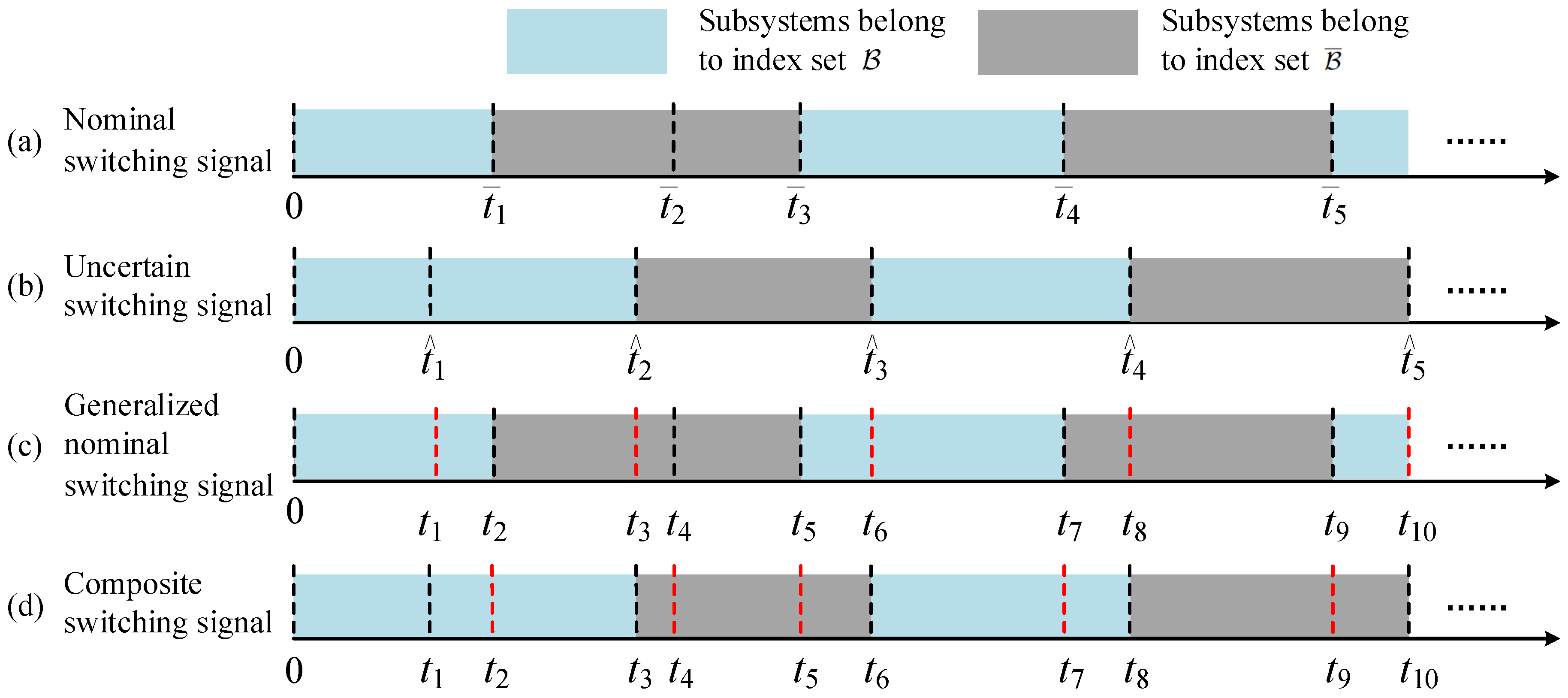
3.2. Stability Under Switching Sequence Uncertainties

This section focuses on the sequence uncertainties that satisfy (12) and (13) in Definition 2, and provides criteria for assessing the robust exponential stability of system (1) using the average dwell time approach.

Definition 4.

For any $t_R>t_L>0$, let $T_{\mathcal{B}}(t_L,t_R)$ (respectively, $T_{\overline{\mathcal{B}}}(t_L,t_R)$) denote the total running time of the modes ${\Pi }_p$, where $p\in \mathcal{B}$ (respectively, $p\in \overline{\mathcal{B}}$), over the interval $[t_L,t_R]$. If there exist positive constants ${\mathrm{N}}_0$ and ${\tau }_{\mathcal{B}}$ (respectively, ${\mathrm{N}}_{1}and{\tau }_{\overline{\mathcal{B}}}$) such that

$${\mathrm{N}}_{\overline{\sigma }}^{\mathcal{B}}(t_L,t_R)\le {\mathrm{N}}_0+{\displaystyle \frac{T_{\mathcal{B}}(t_L,t_R)}{{\tau }_{\mathcal{B}}}}$$

(32)

and

$${\mathrm{N}}_{\overline{\sigma }}^{\overline{\mathcal{B}}}(t_L,t_R)\ge {\mathrm{N}}_1+{\displaystyle \frac{T_{\overline{\mathcal{B}}}(t_L,t_R)}{{\tau }_{\overline{\mathcal{B}}}}}$$

(33)

hold, then ${\tau }_{\mathcal{B}}$ (respectively, ${\tau }_{\overline{\mathcal{B}}}$) is called the average dwell time (respectively, the average dwell time of fast switching) under $\overline{\sigma }\left(t\right)$. Without loss of generality, throughout this paper, ${\mathrm{N}}_0$ and ${\mathrm{N}}_1$ are set to zero.

Theorem 2.

Consider a switched interconnected system (1) where modes satisfy (2)–(6), $\sigma \left(t\right)$ satisfies (7), $\Sigma \left(t\right)$ satisfies (8), and $\rho \left(t\right)$ satisfies (12)–(13). If $\forall p\in \mathcal{B}$ matrix $A_p=\left(a_{ij}^p\right)$ of order $\mathtt{N}$ is a nonsingular M-matrix and

$${\displaystyle \frac{{\tau }_{\mathcal{B}}}{{\tau }_{\overline{\mathcal{B}}}}}>min\left\{{\displaystyle \frac{{\lambda }_{1}c}{\lambda (1-c)}},{\displaystyle \frac{{\lambda }_1(1-d)}{\lambda d}}\right\}$$

(34)

$$ln\kappa +(1-\mathcal{R}){\theta }_1+\mathcal{R}{\theta }_2=-ϵ<0$$

(35)

then for ${\mathit{P}}_{ij}^p\in {\mathit{P}}_{ij}^{I·p}$, ${\mathit{Q}}_{ij}^p\in {\mathit{Q}}_{ij}^{I·p}$, the switched interconnected system (1) is robustly exponentially stable. Where ${\theta }_1=\left[-\lambda (1-c){\tau }_{\mathcal{B}}+{\lambda }_{1}c{\tau }_{\overline{\mathcal{B}}}\right]$, ${\theta }_2=\left[-\lambda d{\tau }_{\mathcal{B}}+{\lambda }_1(1-d){\tau }_{\overline{\mathcal{B}}}\right]$, and

$$\begin{array}{cc}\hfill a_{ii}^p=& {\beta }_{i1}^p{\left({\alpha }_{ih}^p\right)}^{-{\displaystyle \frac{1}{2}}}-{\left({\alpha }_{il}^p\right)}^{-{\displaystyle \frac{1}{2}}}{\gamma }_i^p{L}_{ii}^p\left(∥{\mathit{P}}_{ii}^{p·*}∥+∥{\mathit{Q}}_{ii}^{p·*}∥\right),\hfill \\ \hfill a_{ij}^p=& -{\left({\alpha }_{jl}^p\right)}^{-{\displaystyle \frac{1}{2}}}{\gamma }_i^p{L}_{ij}^p\left(∥{\mathit{P}}_{ij}^{p·*}∥+∥{\mathit{Q}}_{ij}^{p·*}∥\right),i\ne j\hfill \end{array}$$

Proof of Theorem 2.

First, we will examine the system’s behavior at each switching instant $t_k$ ($k=1,2,\dots$) under $\overline{\sigma }\left(t\right)$. Let $\Delta t_{i,\mathcal{B}}$ and $\Delta t_{i,\overline{\mathcal{B}}}$, respectively, denote the ith activating period of modes ${\Pi }_p$, $p\in \mathcal{B}$, and modes ${\Pi }_q$, $q\in \overline{\mathcal{B}}$ under $\overline{\sigma }\left(t\right)$.

It follows from (27) and (31) that, for $t\in [t_k,t_{k+1})$,

$$∥{\mathit{y}}_i\left(t\right)∥<{{\kappa }_1}_p{∥{\mathit{y}}_i\left(s\right)∥}_{t_k}{e}^{-\lambda (t-t_k)/2},\mathrm{if}p\in \mathcal{B}$$

(36)

or

$$∥{\mathit{y}}_i\left(t\right)∥<{{\kappa }_2}_p{∥{\mathit{y}}_i\left(s\right)∥}_{t_k}{e}^{{\lambda }_1(t-t_k)/2},\mathrm{if}p\in \overline{\mathcal{B}}$$

(37)

where ${∥{\mathit{y}}_i\left(s\right)∥}_{t_k}=\underset{j=1,\dots ,n}{max}\left\{{sup}_{s\in \left[t_k-{\tau }^{\sigma \left(t_k\right)},t_k\right]}\left|y_{ij}\left(s\right)\right|\right\}$. Given the continuity of the system state, from (36) and (37), we obtain

$$\begin{array}{cc}\hfill & ∥{\mathit{y}}_i\left(t\right)∥<{\kappa }^{{\mathrm{N}}_{\overline{\sigma }}\left(t\right)}{e}^{-\lambda T_{\mathcal{B}}(t_0,t)+{\lambda }_1{T}_{\overline{\mathcal{B}}}(t_0,t)}{∥{\mathit{\varphi }}_i\left(s\right)∥}_{t_0}\hfill \\ \hfill =& {\kappa }^{{\mathrm{N}}_{\overline{\sigma }}\left(t\right)}{e}^{-\lambda {\sum }_{i=1}^{{\mathrm{N}}_{\overline{\sigma }}^{\mathcal{B}}\left(t\right)}\Delta t_{i,\mathcal{B}}+{\lambda }_1{\sum }_{i=1}^{{\mathrm{N}}_{\overline{\sigma }}^{\overline{\mathcal{B}}}\left(t\right)}\Delta t_{i,\overline{\mathcal{B}}}}{∥{\mathit{\varphi }}_i\left(s\right)∥}_{t_0}\hfill \end{array}$$

(38)

where $\kappa ={max}_{p\in \mathcal{A}}\{{{\kappa }_1}_p,{{\kappa }_2}_p\}$.

By comparing the generalized nominal switching signal $\overline{\Sigma }\left(t\right)$ with the composite switching signal $\overline{\sigma }\left(t\right)$, it is evident that in (38), each of the time intervals $\Delta t_{i,\mathcal{B}}$, where $i=1,2,\dots ,{\mathrm{N}}_{\overline{\sigma }}^{\mathcal{B}}\left(t\right)$, can be classified into the following two cases:

Case 1. When $t\in \Delta t_{i,\mathcal{B}}$, both $\overline{\Sigma }\left(t\right)$ and $\overline{\sigma }\left(t\right)$ belong to $\mathcal{B}$, i.e., $\forall t\in \Delta t_{i,\mathcal{B}}$, the modes ${\Pi }_p\in {\Pi }_{\mathcal{B}}$ are prescribed to be activated under $\overline{\Sigma }\left(t\right)$. In the presence of uncertainties, these modes ${\Pi }_p$ remain activated under $\overline{\sigma }\left(t\right)$. It follows from (12) that the number of these periods is no less than $(1-\mathcal{R})(1-c){\mathrm{N}}_{\overline{\sigma }}\left(t\right){\tau }_{\mathcal{B}}$.

Case 2. When $t\in \Delta t_{i,\overline{\mathcal{B}}}$, $\overline{\Sigma }\left(t\right)$ belongs to $\overline{\mathcal{B}}$, while $\overline{\sigma }\left(t\right)$ belongs to $\mathcal{B}$, i.e., $\forall t\in \Delta t_{i,\overline{\mathcal{B}}}$, the modes ${\Pi }_q\in {\Pi }_{\overline{\mathcal{B}}}$ are prescribed to be activated under $\overline{\Sigma }\left(t\right)$. However, due to switching uncertainties, the modes ${\Pi }_p\in {\Pi }_{\mathcal{B}}$ replace the modes ${\Pi }_q$ under $\overline{\sigma }\left(t\right)$. It follows from (12) that the number of these periods is no less than $\mathcal{R}d{\mathrm{N}}_{\overline{\sigma }}\left(t\right){\tau }_{\mathcal{B}}$.

One further has that

$$T_{\mathcal{B}}(t_0,t)\ge \left[(1-\mathcal{R})(1-c)+\mathcal{R}d\right]{\mathrm{N}}_{\overline{\sigma }}\left(t\right){\tau }_{\mathcal{B}}$$

(39)

Similarly, one also has from (13) that

$$T_{\overline{\mathcal{B}}}(t_0,t)\le \left[\mathcal{R}(1-d)+(1-\mathcal{R})c\right]{\mathrm{N}}_{\overline{\sigma }}\left(t\right){\tau }_{\overline{\mathcal{B}}}$$

(40)

Substituting (39) and (40) into (38) yields

$$\begin{array}{cc}\hfill & ∥{\mathit{y}}_i\left(t\right)∥\hfill \\ \hfill <& {\kappa }^{{\mathrm{N}}_{\overline{\sigma }}\left(t\right)}{e}^{-\lambda T_{\mathcal{B}}(t_0,t)+{\lambda }_1{T}_{\overline{\mathcal{B}}}(t_0,t)}{∥{\mathit{\varphi }}_i\left(s\right)∥}_{t_0}\hfill \\ \hfill \le & e^{{\mathrm{N}}_{\overline{\sigma }}\left(t\right)ln\kappa -\lambda \left[(1-\mathcal{R})(1-c)+\mathcal{R}d\right]{\mathrm{N}}_{\overline{\sigma }}\left(t\right){\tau }_{\mathcal{B}}+{\lambda }_1\left[\mathcal{R}(1-d)+(1-\mathcal{R})c\right]{\mathrm{N}}_{\overline{\sigma }}\left(t\right){\tau }_{\overline{\mathcal{B}}}}{∥{\mathit{\varphi }}_i\left(s\right)∥}_{t_0}\hfill \\ \hfill =& e^{{\mathrm{N}}_{\overline{\sigma }}\left(t\right)\left\{ln\kappa +(1-\mathcal{R})\left[-\lambda (1-c){\tau }_{\mathcal{B}}+{\lambda }_{1}c{\tau }_{\overline{\mathcal{B}}}\right]\right\}}\hfill \\ \hfill & \times e^{{\mathrm{N}}_{\overline{\sigma }}\left(t\right)\left\{\mathcal{R}\left[-\lambda d{\tau }_{\mathcal{B}}+{\lambda }_1(1-d){\tau }_{\overline{\mathcal{B}}}\right]\right\}}{∥{\mathit{\varphi }}_i\left(s\right)∥}_{t_0}\hfill \\ \hfill =& e^{{\mathrm{N}}_{\overline{\sigma }}\left(t\right)[ln\kappa +(1-\mathcal{R}){\theta }_1+\mathcal{R}{\theta }_2]}{∥{\mathit{\varphi }}_i\left(s\right)∥}_{t_0}\hfill \\ \hfill \le & e^{-{\displaystyle \frac{ϵ}{{\tau }_{\overline{\mathcal{B}}}}}(t-t_0)}{∥{\mathit{\varphi }}_i\left(s\right)∥}_{t_0}\hfill \end{array}$$

(41)

Under condition (34), three cases are considered:

Case 1: ${\displaystyle \frac{{\tau }_{\mathcal{B}}}{{\tau }_{\overline{\mathcal{B}}}}}>{\displaystyle \frac{{\lambda }_{1}c}{\lambda (1-c)}}$. There exists a small $\mathcal{R}$ that meets condition (35).

Case 2: ${\displaystyle \frac{{\tau }_{\mathcal{B}}}{{\tau }_{\overline{\mathcal{B}}}}}>{\displaystyle \frac{{\lambda }_1(1-d)}{\lambda d}}$. There exists a large $\mathcal{R}$ that meets condition (35).

Case 3: ${\displaystyle \frac{{\tau }_{\mathcal{B}}}{{\tau }_{\overline{\mathcal{B}}}}}>max\left\{{\displaystyle \frac{{\lambda }_{1}c}{\lambda (1-c)}},{\displaystyle \frac{{\lambda }_1(1-d)}{\lambda d}}\right\}$. In this case, $\mathcal{R}$ can be chosen more flexibly to meet condition (35). □

Remark 6.

In (27) and (31), the amplification factor ${\kappa }_p$ (respectively, ${\kappa }_p^{*}$) characterizes the scaling of the initial condition but does not affect the exponential decay rate λ (respectively, the exponential divergence rate ${\lambda }_1$). Due to the continuity of the system state, the amplification factor at each switching moment can be set to a constant value of 1. Consequently, Equation (41) can be transformed into

$$\begin{array}{c}\hfill ∥{\mathit{y}}_i\left(t\right)∥<{\kappa }_{t_0}{e}^{{\mathrm{N}}_{\overline{\sigma }}\left(t\right)[(1-\mathcal{R}){\theta }_1+\mathcal{R}{\theta }_2]}{∥{\mathit{\varphi }}_i\left(s\right)∥}_{t_0}={\kappa }_{t_0}{e}^{-\vartheta (t-t_0)}{∥{\mathit{\varphi }}_i\left(s\right)∥}_{t_0}\end{array}$$

(42)

where ${\kappa }_{t_0}$ is the amplification factor of the first activated mode and $\vartheta ={\displaystyle \frac{(1-\mathcal{R}){\theta }_1+\mathcal{R}{\theta }_2}{{\tau }_{\overline{\mathcal{B}}}}}$.

Remark 7.

In the study of the stability of switched systems with unstable modes, many works impose constraints on the dwell time of the switching signal, specifically $\Delta t_{min}\le t_{k+1}-t_k\le \Delta t_{max}$, $k=0,1,\dots$, with stability conditions dependent on $\Delta t_{min}$ and/or $\Delta t_{max}$. As a result, if the dwell time of any subsystem is either too short or too long, the stability criteria may fail, making the conditions overly conservative. For instance, in Theorem 2 of [51], if a single subsystem’s dwell time is too short, conditions (7) and (8) become difficult to satisfy. In this paper, we use the average dwell time ratio to determine system stability, which avoids the drawback of stability criteria failing due to excessively short or long dwell times of individual subsystems.

Remark 8.

It follows from the definitions of ${\theta }_1$ and ${\theta }_2$ that ${\theta }_1$ is proportional to c, while ${\theta }_2$ is inversely proportional to d. These relationships imply that condition (35) is satisfied when c is small (reflecting a low switching rate from stable to unstable modes) and d is large (indicating a high switching rate from unstable to stable modes).

Remark 9.

It is well known that in the stability analysis of switched systems with unstable subsystems, stability can be achieved if the activation time of the stable subsystems is sufficiently long, such that the decay of the stable subsystems to compensate for the divergence caused by the activation of the unstable subsystems [8,9,10]. When $\rho \left(t\right)\equiv 0$, i.e., $\Sigma \left(t\right)\equiv \sigma \left(t\right)$, condition (35) becomes

$$-ln\kappa +(1-\mathcal{R})\lambda {\tau }_{\mathcal{B}}-\mathcal{R}{\lambda }_1{\tau }_{\overline{\mathcal{B}}}>0.$$

(43)

This is consistent with the results presented in [8,9,10]. However, this property becomes more subtle when disturbances are present in the switching signal, as the prescribed stable modes may be replaced by unstable ones, and vice versa. Moreover, the ratios and activating times of stable and unstable modes can be adjusted to satisfy condition (35) for system stability, depending on the values of ${\theta }_1$ and ${\theta }_2$. For example, when c is sufficiently small, meaning that the ratio of change from stable to unstable modes is sufficiently small. It is possible to select a small value for $\mathcal{R}$ and set large (or small) prescribed activation times for stable (or unstable) modes to satisfy condition (35). This corresponds to the case where ${\theta }_1<0$ and ${\theta }_2>0$.

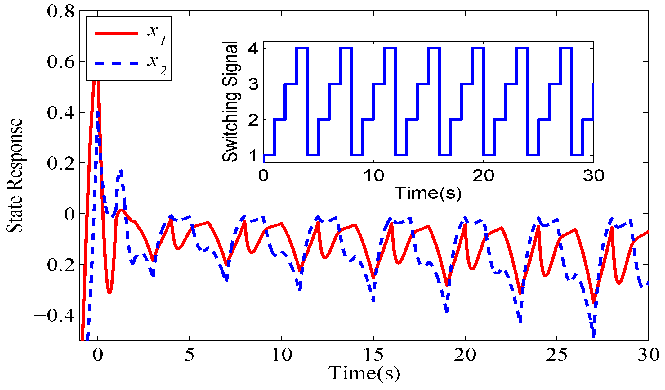
4. Numerical Example

To demonstrate the validity and applicability of the theoretical findings, we provide the following example.

Example 1.

Artificial neural networks, being typical interconnected systems, have attracted significant research interest owing to their successful applications in various fields, including dynamic optimization, associative memory, and pattern recognition. The following illustrates a model of two-neuron switched neural networks with four modes. Modes 1 and 2 are taken from [52], while modes 3 and 4 are from [53].

$${\dot{x}}_i\left(t\right)=-e_i^{\sigma \left(t\right)}{x}_i\left(t\right)+\sum _{j=1}^2{b}_{ij}^{\sigma \left(t\right)}{g}_j^{\sigma \left(t\right)}\left(x_j\left(t\right)\right)+\sum _{j=1}^2{c}_{ij}^{\sigma \left(t\right)}{g}_j^{\sigma \left(t\right)}\left(x_j\left(t-{\tau }_{ij}^{\sigma \left(t\right)}\left(t\right)\right)\right)$$

(44)

where

$$g_j^p\left(x_j\right)=0.5x_j+0.5sin{x}_j,{\tau }_{ij}^p=1,i,j,p=1,2$$

$$g_j^q\left(x_j\right)=tanh{x}_j,{\tau }_{ij}^q=e^t/(1+e^t),i,j=1,2,q=3,4;$$

$${\mathit{E}}^{I·1}=\left[\begin{array}{cc}\left[3.994.01\right]& 0\\ 0& \left[2.993.01\right]\end{array}\right],{\mathit{E}}^{I·2}=\left[\begin{array}{cc}\left[2.812.95\right]& 0\\ 0& \left[3.603.72\right]\end{array}\right],$$

$${\mathit{B}}^{I·1}=\left[\begin{array}{cc}\left[1.191.21\right]& \left[2.352.41\right]\\ \left[0.050.06\right]& \left[0.030.04\right]\end{array}\right],{\mathit{B}}^{I·2}=\left[\begin{array}{cc}\left[0.871.01\right]& \left[0.030.10\right]\\ \left[2.072.28\right]& \left[0.680.80\right]\end{array}\right],$$

$${\mathit{C}}^{I·1}=\left[\begin{array}{cc}\left[0.090.11\right]& \left[3.1403.32\right]\\ \left[-0.050.13\right]& \left[0.430.54\right]\end{array}\right],{\mathit{C}}^{I·2}=\left[\begin{array}{cc}\left[0.110.35\right]& \left[-0.020.10\right]\\ \left[2.873.00\right]& \left[0.050.13\right]\end{array}\right],$$

$${\mathit{E}}^3=\left[\begin{array}{cc}0.1& 0\\ 0& 0.1\end{array}\right],{\mathit{B}}^3=\left[\begin{array}{cc}-0.2& 1\\ 1& -0.1\end{array}\right],{\mathit{C}}^3=\left[\begin{array}{cc}-0.4& 0.3\\ 0.1& 0.6\end{array}\right],$$

$${\mathit{E}}^4=\left[\begin{array}{cc}0.1& 0\\ 0& 0.1\end{array}\right],{\mathit{B}}^4=\left[\begin{array}{cc}0.1& -1.9\\ 0.1& -2.4\end{array}\right],{\mathit{C}}^4=\left[\begin{array}{cc}0.3& -1\\ 0.3& -0.4\end{array}\right],$$

By simple calculation yields

$${\underline{\mathit{E}}}^{1·*}=\left[\begin{array}{cc}3.99& 0\\ 0& 2.99\end{array}\right],{\mathit{B}}^{1·*}=\left[\begin{array}{cc}1.21& 2.41\\ 0.06& 0.04\end{array}\right],{\mathit{C}}^{1·*}=\left[\begin{array}{cc}0.11& 3.32\\ 0.13& 0.54\end{array}\right],$$

$${\underline{\mathit{E}}}^{2·*}=\left[\begin{array}{cc}2.81& 0\\ 0& 3.60\end{array}\right],{\mathit{B}}^{2·*}=\left[\begin{array}{cc}1.01& 0.10\\ 2.28& 0.80\end{array}\right],{\mathit{C}}^{2·*}=\left[\begin{array}{cc}0.35& 0.10\\ 3.00& 0.13\end{array}\right],$$

and $A_1$ and $A_2$ are M-matrices, while $A_3$ and $A_4$ are not M-matrices. Therefore, ${\Pi }_1,{\Pi }_2\in {\Pi }_{\mathcal{B}}$ and ${\Pi }_3,{\Pi }_4\in {\Pi }_{\overline{\mathcal{B}}}$. From Equation (17), it can be estimated that $\lambda =0.92$. Additionally, based on the states of modes ${\Pi }_3$ and ${\Pi }_4$, ${\lambda }_1$ is estimated to be $0.15$. For numerical simulations, let ${\mathit{E}}^i={\underline{\mathit{E}}}^{i·*}$, ${\mathit{B}}^i={\mathit{B}}^{i·*}$, and ${\mathit{C}}^i={\mathit{C}}^{i·*}$, $i=1,2$ with initial condition $[cos(2s)-0.4,sin(2s)+0.4]$.

Figure 2, Figure 3, Figure 4 and Figure 5 show the state responses of the four modes. The simulation results verify that modes ${\Pi }_1$ and ${\Pi }_2$ are stable, while mode ${\Pi }_3$ and mode ${\Pi }_4$ are unstable. An inappropriate switching signal may cause system (44) to become unstable, as shown in Figure 6 and Figure 7.

Design a nominal switching signal $\Sigma \left(t\right)$ to stabilize the system (44), i.e., $\forall t\in [10k,2+10k]$, $\Sigma \left(t\right)=1$; $t\in [2+10k,6+10k]$, $\Sigma \left(t\right)=2$; $t\in [6+10k,8+10k]$, $\Sigma \left(t\right)=3$; $t\in [8+10k,10+10k]$, $\Sigma \left(t\right)=4$; $k=0,1,\dots$, and let $\mathcal{R}=0.5$. As depicted in Figure 8, the system rapidly converges to the equilibrium point $\mathit{x}=\mathbf{0}$ under the nominal switching signal $\Sigma \left(t\right)$.

Next, we will examine whether the nominal switching signal $\Sigma \left(t\right)$ can still stabilize system (44) in the presence of uncertain disturbances, which result in $c=0.6$, $d=0.4$, and a $0.5s$ delay in the switching signal. According to condition (34) of Theorem 2, system (44) will remain exponentially stable when ${\displaystyle \frac{{\tau }_{\mathcal{B}}}{{\tau }_{\overline{\mathcal{B}}}}}>{\displaystyle \frac{{\lambda }_1(1-d)}{\lambda d}}=0.25$. Since $c=0.6$, $d=0.4$, and $\mathcal{R}=0.5$, the stable (unstable) modes in the nominal switching signal are replaced by the unstable (stable) modes. The $0.5s$ delay in the switching signal causes the composite switching signal $\overline{\sigma }\left(t\right)$ (generalized nominal switching signal $\overline{\Sigma }\left(t\right)$) to experience twice as many switching occurrences. One further has that ${\displaystyle \frac{{\tau }_{\mathcal{B}}}{{\tau }_{\overline{\mathcal{B}}}}}={\displaystyle \frac{9.5}{19.5}}=0.49>0.25$. Therefore, it is concluded that system (44) is robustly exponentially stable. Figure 9 and Figure 10 shows that the exponential stability is still achieved under $\overline{\sigma }\left(t\right)$.

5. Conclusions

This paper proposed robust stability conditions for switched interconnected systems with unstable modes, time-varying state delays, and uncertainties in both parameters and switching. By introducing two novel concepts—the generalized nominal switching signal and the composite switching signal—along with a new index called the generalized mode changing rate, this study effectively addresses the impact of switching uncertainties on system stability. By using vector Lyapunov functions and the average dwell time method, sufficient conditions for ensuring the robust exponential stability of the system are derived. Finally, numerical examples demonstrate the effectiveness and validity of the proposed theory. The results show that the proposed theory not only accurately characterizes the robust stability of the system but also provides an effective analytical design approach for interconnected systems with switching uncertainties and time-varying delays in practical applications.

References

1. Liberzon, D.; Morse, A.S. Basic problems in stability and design of switched systems. IEEE Control Syst. Mag. 1999, 19, 59–70. [Google Scholar]
2. Daafouz, J.; Riedinger, P.; Iung, C. Stability analysis and control synthesis for switched systems: A switched Lyapunov function approach. IEEE Trans. Autom. Control 2002, 47, 1883–1887. [Google Scholar] [CrossRef]
3. Xue, H.; Xu, X.; Zhang, J.; Yang, X. Robust stability of impulsive switched neural networks with multiple time delays. Appl. Math. Comput. 2019, 359, 456–475. [Google Scholar] [CrossRef]
4. Xue, H.; Zhang, J. Robust exponential stability of interconnected switched systems with mixed delays and impulsive effect. Nonlinear Dynam. 2019, 97, 679–696. [Google Scholar] [CrossRef]
5. Li, Y.; Xue, H. Robust stability analysis of switched neural networks with application in psychological counseling evaluation system. Mathematics 2024, 12, 2097. [Google Scholar] [CrossRef]
6. Il’in, A.V.; Mosolova, Y.M.; Fomichev, V.V.; Fursov, A.S. On the problem of switched system stabilization. Moscow Univ. Comput. Math. Cybern. 2024, 48, 303–316. [Google Scholar] [CrossRef]
7. Zhai, G.; Hu, B.; Yasuda, K.; Michel, A.N. Stability analysis of switched systems with stable and unstable subsystems: An average dwell time approach. Int. J. Syst. Sci. 2001, 32, 1055–1061. [Google Scholar] [CrossRef]
8. Yang, H.; Jiang, B.; Cocquempot, V. A survey of results and perspectives on stabilization of switched nonlinear systems with unstable modes. Nonlinear Anal. Hybrid Syst. 2014, 13, 45–60. [Google Scholar] [CrossRef]
9. Yang, H.; Cocquempot, V.; Jiang, B. On stabilization of switched nonlinear systems with unstable modes. Syst. Control Lett. 2009, 58, 703–708. [Google Scholar] [CrossRef]
10. Zhang, M.; Gao, L. Input-to-state stability for impulsive switched nonlinear systems with unstable subsystems. Trans. Inst. Meas. Control 2018, 40, 2167–2177. [Google Scholar] [CrossRef]
11. Xing, J.; Wu, B.; Wang, Y.; Liu, L. Exponential stability and non-weighted L2-gain analysis for switched neutral systems with unstable subsystems. Int. J. Syst. Sci. 2025, 56, 673–689. [Google Scholar] [CrossRef]
12. Li, H.; Wei, Z. Stability analysis of discrete-time switched systems with all unstable subsystems. Discrete Contin. Dyn. Syst.-S 2024, 17, 2762–2777. [Google Scholar] [CrossRef]
13. Zhang, N.; Sun, Y. Stabilization of switched positive linear delay system with all subsystems unstable. Int. J. Robust Nonlinear Control 2024, 34, 2441–2456. [Google Scholar] [CrossRef]
14. Zhang, L.X.; Gao, H.J. Asynchronously switched control of switched linear systems with average dwell time. Automatica 2010, 46, 953–958. [Google Scholar] [CrossRef]
15. Zong, G.; Wang, R.; Zheng, W.X.; Hou, L. Finite-time stabilization for a class of switched time-delay systems under asynchronous switching. Appl. Math. Comput. 2013, 219, 5757–5771. [Google Scholar] [CrossRef]
16. Wu, X.; Tang, Y.; Cao, J.; Zhang, W. Distributed consensus of stochastic delayed multi-agent systems under asynchronous switching. IEEE Trans. Cybern. 2015, 46, 1817–1827. [Google Scholar] [CrossRef] [PubMed]
17. Liu, L.; Deng, F. Stability and stabilization of nonlinear stochastic systems with synchronous and asynchronous switching parameters to the states. IEEE Trans. Cybern. 2022, 53, 4894–4907. [Google Scholar] [CrossRef]
18. Zhang, S.; Nie, A.B. Exponential stability of fractional-order uncertain systems with asynchronous switching and impulses. Int. J. Robust Nonlinear Control 2024, 34, 7285–7313. [Google Scholar] [CrossRef]
19. Hu, B.; Xu, X.; Antsaklis, P.J.; Michel, A.N. Robust stabilizing control laws for a class of second-order switched systems. Syst. Control Lett. 1999, 38, 197–207. [Google Scholar] [CrossRef]
20. Hetel, L.; Daafouz, J.; Iung, C. Stability analysis for discrete time switched systems with temporary uncertain switching signal. In Proceedings of the 46th IEEE Conference on Decision and Control, New Orleans, LA, USA, 12–14 December 2007; pp. 5623–5628. [Google Scholar]
21. Li, Z.G.; Soh, Y.C.; Wen, C.Y. Robust stability of quasi-periodic hybrid dynamic uncertain systems. IEEE Trans. Autom. Control 2001, 46, 107–111. [Google Scholar] [CrossRef]
22. Sun, Z. Robust switching of discrete-time switched linear systems. Automatica 2012, 48, 239–242. [Google Scholar] [CrossRef]
23. Han, T.-T.; Ge, S.S.; Lee, T.H. Adaptive neural control for a class of switched nonlinear systems. Syst. Control Lett. 2009, 58, 109–118. [Google Scholar] [CrossRef]
24. Yang, H.; Jiang, B.; Tao, G.; Zhou, D. Robust stability of switched nonlinear systems with switching uncertainties. IEEE Trans. Autom. Control 2016, 61, 2531–2537. [Google Scholar] [CrossRef]
25. Zhang, L.; Boukas, E. Stability and stabilization of Markovian jump linear systems with partly unknown transition probabilities. Automatica 2009, 45, 463–468. [Google Scholar] [CrossRef]
26. Xiang, W.; Lam, J.; Li, P. On stability and H control of switched systems with random switching signals. Automatica 2018, 95, 419–425. [Google Scholar] [CrossRef]
27. Roy, S.; Baldi, S.; Ioannou, P.A. An adaptive control framework for underactuated switched Euler–Lagrange systems. IEEE Trans. Autom. Control 2021, 67, 4202–4209. [Google Scholar] [CrossRef]
28. Brodtkorb, A.H.; Værnø, S.A.; Teel, A.R.; Sørensen, A.J.; Skjetne, R. Hybrid controller concept for dynamic positioning of marine vessels with experimental results. Automatica 2018, 93, 489–497. [Google Scholar] [CrossRef]
29. Mahmoud, M.S.; AL-Sunni, F.M. Interconnected continuous-time switched systems: Robust stability and stabilization. Nonlinear Anal. Hybrid Syst. 2010, 4, 531–542. [Google Scholar] [CrossRef]
30. Long, L.; Zhao, J. A small-gain theorem for switched interconnected nonlinear systems and its applications. IEEE Trans. Autom. Control 2013, 59, 1082–1088. [Google Scholar] [CrossRef]
31. Long, L. Multiple Lyapunov functions-based small-gain theorems for switched interconnected nonlinear systems. IEEE Trans. Autom. Control 2017, 62, 3943–3958. [Google Scholar] [CrossRef]
32. Hou, Y.; Liu, Y.-J.; Tong, S. Decentralized event-triggered fault-tolerant control for switched interconnected nonlinear systems with input saturation and time-varying full-state constraints. IEEE Trans. Fuzzy Syst. 2024, 32, 3850–3860. [Google Scholar] [CrossRef]
33. Gurrala, G.; Sen, I. Power system stabilizers design for interconnected power systems. IEEE Trans. Power Syst. 2010, 25, 1042–1051. [Google Scholar] [CrossRef]
34. Li, Y.M.; Tong, S.C. Adaptive neural networks prescribed performance control design for switched interconnected uncertain nonlinear systems. IEEE Trans. Neural Netw. Learn. Syst. 2018, 29, 3059–3068. [Google Scholar] [CrossRef]
35. Zhao, Y.W.; Zhang, H.Y.; Chen, Z.Y.; Wang, H.Q.; Zhao, X.D. Adaptive neural decentralised control for switched interconnected nonlinear systems with backlash-like hysteresis and output constraints. Int. J. Syst. Sci. 2022, 53, 1545–1561. [Google Scholar] [CrossRef]
36. Zhai, D.; Liu, X.; Liu, Y.J. Adaptive decentralized controller design for a class of switched interconnected nonlinear systems. IEEE Trans. Cybern. 2020, 50, 1644–1654. [Google Scholar] [CrossRef]
37. Zhang, J.; Li, S.; Ahn, C.K.; Xiang, Z.R. Adaptive fuzzy decentralized dynamic surface control for switched large-scale nonlinear systems with full-state constraints. IEEE Trans. Cybern. 2022, 52, 10761–10772. [Google Scholar] [CrossRef]
38. Chen, Y. Fuzzy interactions compensation in adaptive control of switched interconnected systems. IEEE Trans. Autom. Sci. Eng. 2024, 21, 48–55. [Google Scholar] [CrossRef]
39. Song, Y.; Liu, Y.; Zhao, W. Approximately bi-similar symbolic model for discrete-time interconnected switched system. IEEE/CAA J. Autom. Sinica 2024, 11, 2185–2187. [Google Scholar] [CrossRef]
40. Jonsson, U.T.; Kao, C.Y.; Fujioka, H. Low dimensional stability criteria for large-scale interconnected systems. In Proceedings of the 9th European Control Conference, Kos, Greece, 2–5 July 2007; pp. 2741–2747. [Google Scholar]
41. Andersen, M.S.; Pakazad, S.K.; Hansson, A.; Rantzer, A. Robust stability analysis of sparsely interconnected uncertain systems. IEEE Trans. Autom. Control 2014, 59, 2151–2156. [Google Scholar] [CrossRef]
42. Thanh, N.T.; Phat, V.N. Decentralized stability for switched nonlinear large-scale systems with interval time-varying delays in interconnections. Nonlinear Anal. Hybrid Syst. 2014, 11, 22–36. [Google Scholar] [CrossRef]
43. Ren, H.; Zong, G.; Hou, L.; Yi, Y. Finite-time control of interconnected impulsive switched systems with time-varying delay. Appl. Math. Comput. 2016, 276, 143–157. [Google Scholar] [CrossRef]
44. Malloci, I.; Lin, Z.; Yan, G. Stability of interconnected impulsive switched systems subject to state dimension variation. Nonlinear Anal. Hybrid Syst. 2012, 6, 960–971. [Google Scholar] [CrossRef]
45. Yang, G.; Liberzon, D. A Lyapunov-based small-gain theorem for interconnected switched systems. Syst. Control Lett. 2015, 78, 47–54. [Google Scholar] [CrossRef]
46. Cao, J.; Huang, D.; Qu, Y. Global robust stability of delayed recurrent neural networks. Chaos Solitons Fractals 2005, 23, 221–229. [Google Scholar] [CrossRef]
47. Ensari, T.; Arik, S. New results for robust stability of dynamical neural networks with discrete time delays. Expert Syst. Appl. 2010, 37, 5925–5930. [Google Scholar] [CrossRef]
48. Faydasicok, O.; Arik, S. A new upper bound for the norm of interval matrices with application to robust stability analysis of delayed neural networks. Neural Netw. 2013, 44, 64–71. [Google Scholar] [CrossRef] [PubMed]
49. Siljak, D.D. Large Scale Dynamic Systems: Stability and Structure; IEEE: Amsterdam, The Netherlands, 1978. [Google Scholar]
50. Li, X.; Cao, J.; Perc, M. Switching laws design for stability of finite and infinite delayed switched systems with stable and unstable modes. IEEE Access 2018, 6, 6677–6691. [Google Scholar] [CrossRef]
51. Wang, Y.-E.; Karimi, H.R.; Wu, D. Conditions for the stability of switched systems containing unstable subsystems. IEEE Trans. Circuits Syst. II Express Briefs 2019, 66, 653–657. [Google Scholar] [CrossRef]
52. Xue, H.; Zhang, J.; Wang, H.; Jiang, B. Robust stability of switched interconnected systems with time-varying delays. J. Comput. Nonlinear Dyn. 2018, 13, 021004. [Google Scholar] [CrossRef]
53. Qi, J.; Li, C.; Huang, T.; Zhang, W. Exponential stability of switched time-varying delayed neural networks with all modes being unstable. Neural Process. Lett. 2016, 43, 553–565. [Google Scholar] [CrossRef]
Figure 1. Nominal switching signal, uncertain switching signal, generalized nominal switching signal, and composite switching signal.
Mathematics 13 01554 g001
Figure 2. State responses of mode 1 of the considered switched system.
Mathematics 13 01554 g002
Figure 3. State responses of mode 2 of the considered switched system.
Mathematics 13 01554 g003
Figure 4. State responses of mode 3 of the considered switched system.
Mathematics 13 01554 g004
Figure 5. State responses of mode 4 of the considered switched system.
Mathematics 13 01554 g005
Figure 6. Unstable switching signal for system (44).
Mathematics 13 01554 g006
Figure 7. Unstable switching signal for system (44).
Mathematics 13 01554 g007
Figure 8. Unstable switching signal for system (44).
Mathematics 13 01554 g008
Figure 9. Unstable switching signal for system (44).
Mathematics 13 01554 g009
Figure 10. Unstable switching signal for system (44).
Mathematics 13 01554 g010
Disclaimer/Publisher’s Note: The statements, opinions and data contained in all publications are solely those of the individual author(s) and contributor(s) and not of MDPI and/or the editor(s). MDPI and/or the editor(s) disclaim responsibility for any injury to people or property resulting from any ideas, methods, instructions or products referred to in the content.