Article

A Heuristic Approach for Last-Mile Delivery with Consistent Considerations and Minimum Service for a Supply Chain

by
Esteban Santana Contreras
1,
John Willmer Escobar
2,* and
Rodrigo Linfati
3,*
1
School of Industrial Engineering, Universidad del Bío-Bío, Concepción 4030000, Chile
2
Department of Accounting and Finance, Universidad del Valle, Cali 760001, Colombia
3
Departamento de Ingeniería Industrial, Universidad del Bío-Bío, Concepción 4030000, Chile
*
Authors to whom correspondence should be addressed.
Mathematics 2025, 13(10), 1553; https://doi.org/10.3390/math13101553
Submission received: 19 March 2025 / Revised: 18 April 2025 / Accepted: 20 April 2025 / Published: 8 May 2025

Abstract

:
This paper considers the problem of consistent routing with minimum service (ConVRPms). ConVRPms aims to determine the minimum cost routes for each day of a planning horizon. In particular, the goal is to satisfy all individual demands and serve every customer via a single driver, with times that do not differ by more than L time units. There is a fleet of homogeneous vehicles that start from a single depot. In this paper, a heuristic algorithm for ConVRPms is proposed. The algorithm is based on classical constructive heuristics and the tabu search metaheuristic. The proposed algorithm has been tested on benchmark instances from the literature. The experimental results show that the proposed approach produces high-quality solutions within computing times considerably less than those observed with CPLEX. The proposed algorithm can optimally solve instances with 20 customers and a planning horizon of three days, producing more economical solutions in some of the larger instances and those requiring hourly consistency ( L = 1   h ).

1. Introduction

In modern industries, companies seek to highlight their efficiency by implementing differentiation strategies. Some companies seek to develop a competitive advantage by delivering higher-quality service and developing loyalty ties with their customers. The consistency of delivery is a fundamental factor to consider in increasing the quality of service, especially for courier service companies, package distribution, health and home care, and cleaning services. Ref. [1] argued that ensuring consistent schedules and limiting the number of drivers with which a customer must interact can significantly improve customer satisfaction, facilitate reception operations, and improve trust between the company and the customer.
Researchers have proposed solution strategies to increase the quality of periodic service and minimize the impact of operational costs. Ref. [2] introduced the Consistent Vehicle Routing Problem (ConVRP), inspired by the courier and parcel delivery industry. The ConVRP is a variant of the well-known vehicle routing problem (VRP), which is focused primarily on customer satisfaction through consistent periodic service. In the ConVRP, the objective is to determine the routes to be performed with the minimum cost for a fleet of homogeneous vehicles operating daily within a planning horizon. The ConVRP seeks to satisfy all the demands, and a single driver/supplier must regularly serve each customer for multiple periodic visits.
Given its economic relevance, applicability, and complexity, the ConVRP has been studied by multiple researchers, who have proposed various variants and applications of the problem, and heuristic or exact algorithms for its solution. The ConVRP has been classified as NP-hard [2]. Ref. [2] indicates that the constraints associated with temporal consistency significantly complicate the problem’s solution since they introduce interdependencies between the routes for multiple days.
Ref. [3] introduced the Consistent Vehicle Routing Problem with Minimum Service (ConVRPms). Unlike the traditional ConVRP, the ConVRP considers that the number of vehicles is defined a priori, and that each driver/supplier must serve at least one customer on each day of the planning horizon. The ConVRPms is a combinatorial optimization problem aimed at increasing consumer satisfaction through the delivery of a periodic service through the same driver/supplier and at regular times. Ref. [3] designed a set of small, structured instances for ConVRPms, in which the efficiency of an exact branch-and-cut method was tested. ConVRPms is a problem whose application is helpful for the operational planning of the courier service and package distribution industries, determining high-quality routes and meeting the essential criteria of the ConVRP.
The main contribution of this paper is the proposal of a heuristic solution method for ConVRPms that produces high-quality solutions within short computing times for large instances. The general motivation of the paper is to introduce an efficient approach to solving several variants of the vehicle routing problem, considering the consistency of the driver and the time to be visited. This approach could be applied to several industries related to health delivery problems for medication and patient visits. In the literature review, there are no published efficient algorithms that are based on heuristic approaches for solving the ConVRPms. The former algorithm is deterministic and considers a sequential structure. The proposed approach involves constructive heuristics and local search procedures based on a tabu search (TS) metaheuristic. TS has been selected because of its excellent performance in solving several complex variants of the well-known VRP [4,5]. Indeed, the TS approach is easy to implement, and the short-term memory generates an extraordinary exploration of the search space, avoiding local optima. In addition, its intensification strategy allows the proposed approach to obtain high-quality solutions within short computing times. The proposed strategy could be extended to the solution of current and future variants of the ConVRP, contributing to a reference framework for future research.

2. Literature Review

Vehicle routing problems are a family of combinatorial optimization problems that seek to determine the routes of a set of vehicles to serve a set of customers. Generally, the objective of such problems is to minimize the total operation cost or transit time. However, the objective and its constraints depend on the specific characteristics of the problem. The ConVRP is a variant of the traditional VRP that seeks consistency in visits to customers because visits on routes must be performed by the same driver and at the same hour.
Ref. [2] introduced the Consistent Vehicle Routing Problem (ConVRP) inspired by the courier and parcel delivery industry. In this work, an arc-based mixed-integer programming model is formulated, and a two-stage heuristic method (ConRTR) is introduced. A set of routes is generated in the first instance, including all recurring customers. Then, the routes are scheduled each day from the initial routes, scheduling the daily demands of nonrecurring customers. The routes are improved via local search. A tabu search approach based on the concept of template routes ([2]) for the solution of the ConVRP was proposed by [6]. The proposed method adopts a two-level master–slave decomposition scheme. Initially, a master template is built to determine the sequence of delivered services to frequent customers for the planning horizon. An enhancement method based on tabu search modifies template routes and daily service schedules sequentially. The algorithm’s performance was compared on a set of instances introduced by [2].
Ref. [1] introduced the time-consistent vehicle routing problem (TCVRP), which focuses on transportation services for people with disabilities. This paper proposes a heuristic algorithm based on large neighborhood search (LNS), in which a VRP with time windows (VRPTW) without waiting times is solved. The performance of the LNS is compared with that of CPLEX for the set of instances designed by [2] and modified for the TCVRP.
Ref. [7] propose the generalized and multiobjective version of the ConVRP, in which the consistency constraints are relaxed, allowing a limited number of drivers per customer and the service schedule within any time window. In this work, an algorithm based on LNS is proposed for solving the problem, and 2-opt operators are applied to improve the consistency of the arrival times. On the other hand, a variable neighborhood search (VNS) for the approximate solution of the ConVRP was developed by [8]. The proposed algorithm considers two sequential phases. In the first phase, an initial solution is obtained that may be infeasible. In the second phase, the solution is repaired and improved in terms of quality. In addition, a special perturbation method has been proposed to diversify the search space. The performance of the VNS is compared with that of other previously published algorithms. The results show that the VNS performs better than the methods proposed by [2,6,7].
Ref. [9] proposes an alternative mathematical formulation for the ConVRP on the basis of sets of customers. For the solution of the model, a method based on column generation (CCG) is proposed. The CCG solves optimality instances with up to 30 customers within less than an hour, outperforming the efficiency of the arc-based model formulated by [2]. An LNS-based approach is proposed that is capable of generating higher-quality solutions within short computing times. Ref. [10] proposed the periodic vehicle routing problem with driver consistency (PVRP-DC). The problem is a variant of the PVRP, in which the same driver must serve every customer in the planning horizon. An algorithm based on branch-and-cut and a family of valid inequalities has been proposed to strengthen the linear relaxation of the problem. A set of 240 instances ranging from 10 to 70 customers is proposed, and the planning horizon varies between two and five days.
Ref. [11] introduces the ConVRP considering profits (ConVRP-Profit), whose objective is to determine the routes that maximize net profit while satisfying capacity, duration (DC), and consistency (ATC) constraints. An adaptive tabu search, which uses short- and long-term memory structures to guide the search process to solve the problem, has been proposed. The algorithm’s efficiency is tested on a set of instances taken from the literature and a new set of instances. The experimental results demonstrated the algorithm’s effectiveness, generating optimal solutions for small-size instances and achieving good performance for large-size instances.
Ref. [3] proposed a variant of the ConVRP, including minimum service constraints (ConVRPms). In this work, a mathematical model for the ConVRPms is formulated. A set of structured instances has been designed to analyze the model’s behavior concerning the number or geographic distribution of customers, the location of the depot, or the required level of consistency for arrival times. The performance of the commercial CPLEX and Gurobi solvers was compared with that of fully relaxed ATC constraints, generating solutions of equal quality and negligible differences within similar computing times.
Ref. [12] considers the consistent vehicle routing problem with time windows (ConVRPTW) motivated by the real application of a food distribution company. Unlike the original ConVRP, this variant relaxes the constraint that every customer is served regularly for the planning horizon. In particular, all the daily demands must be satisfied within the time intervals defined a priori. The objective of the problem is to reduce the total number of vehicles to be used to satisfy the demands for the planning horizon. This paper proposes a heuristic algorithm for the ConVRPTW based on an insertion heuristic to generate an initial solution and a set of heuristics for route elimination. Ref. [13] proposes a mathematical model for the ConVRP considering customers with multiple daily deliveries and other service level agreements, such as time windows and release dates. A decomposition approach is used to solve the considered problem. The proposed approach can solve large-size instances for real-life scenarios. Significant improvements in the total distance traveled and travel times are achieved.
Recently, published works addressing variants of the ConVRP have been proposed by [14,15,16,17,18,19]. A mixed-integer linear programming model and variable neighborhood search metaheuristic with several neighborhood structures for the ConVRP were proposed by [14].
A centrally organized multiperiod collaborative vehicle routing problem, where carriers can exchange customers who have to be served regularly, has been considered by [15]. This problem considers the basic aspects of the ConVRP, adding collaboration work to maintain the workload balance on routes (collaborative-consistent vehicle routing problem with workload balance—CWBConVRP). The authors propose a mathematical model including several valid inequalities for small-size instances. For large instances, an efficient iterated local search algorithm is developed. A variant of the ConVRP considering path consistency based on the underlying road network (ConVRPRN) was studied by [16]. The ConVRPRN considers a set of consistent vehicle routes within a certain period. The objective is to minimize the total travel costs while considering the discount for the paths’ consistent parts. A set-partitioning and a general-arc-flow model are proposed, which are solved by a branch-price-and-cut algorithm.
The ConVRP, with stochastic considerations of the demands, travel times, and service times, was studied by [17]. A hybrid algorithm with a large neighborhood search and simulated annealing is designed to address the proposed NP-hard problem. The Consistent Electric-Vehicle Routing problem with Backhauls and Charging Management was studied by [18]. Finally, the ConVRP considering heterogeneous fleets was introduced by [19].
The latest works considering variants of the ConVRP have been applied by [20,21,22]. Ref. [20] proposes an approach based on a real case for a company in the cleaning sector. The authors decompose the problem into two subproblems, namely, the planning and routing optimization subproblems. A large neighborhood search is applied for the considered problem. Ref. [21] proposed a POPMUSIC-based decomposition of a variable neighborhood search (VNS) scheme for a large-scale consistent vehicle routing problem. The former algorithm is constructive and consequently solves several subproblems to improve the current solution. Ref. [22] consider the problem of shops starting collaboration on urban same-day delivery by using shared vehicles and microdepots for the consolidated transportation of parcels. Consistent routes are designed to simplify the distribution process. The authors propose a two-stage stochastic model for the considered problem. The first stage determines the type of vehicle assigned, and the second optimizes the distribution of the orders.
Ref. [23] addresses a new consistent vehicle routing problem (ConVRP) by considering driver equity and flexible route consistency. For this variant, a flexible strategy to attain route consistency is introduced to traverse as many familiar routes as possible during the planning period by offering time discounts for routes crossed more than twice. A tailored adaptive large neighborhood search algorithm (ALNS) is developed to solve practical-sized problems. Ref. [24] considers stochastic aspects for customers within the ConVRP; a two-stage model, where the first stage assigns customers to drivers and in the second-stage customers are selected for each scenario. Ref. [25] proposes an exact algorithm based on a set-partitioning formulation and robust column and-cut generation for a workload-consistent vehicle routing problem with priority distribution and demand uncertainty.
The literature review revealed that no similar works have been introduced; however, efficient attempts based on heuristic algorithms for solving large-size instances of ConVRPms have been reported. The latest approaches have considered real applications for variants of the ConVRP, algorithms for large-size problems, and some exact approaches. However, exact approaches can solve small- to medium-sized problems within reasonable computing times. On the other hand, real applications are considered only to solve a specific problem, which could be difficult to extend to other variants. Finally, the approaches for solving large instances are close to being implemented for rich vehicle routing problems. We have developed an efficient approach for solving ConVRPms by combining local search procedures within a tabu search scheme.

3. Proposed Approach

3.1. Description of the ConVRPms

The ConVRP variant proposed by [3] aims to determine the minimum cost routes for each day of a planning horizon. In particular, the goal is to satisfy all individual demands and serve every customer via a single driver (DC constraint), with times that do not differ by more than L time units (ATC constraint).
There is a fleet of homogeneous vehicles. The total number of customer products requested for a day by the customers assigned to a vehicle on a given day must be at most its load capacity Q . The number of products demanded by each customer can vary on different days. Each driver must serve at least one customer on each day of the planning horizon, and each route must begin and end at a single depot. The duration of any route must be, at most, the time limit of operation of T time units. The time to deliver the service to a customer can vary within the planning horizon. Upon concluding the service delivery to the customer, the driver must move immediately to the next customer or the depot. Vehicle drivers must not continue in the middle of the route to wait.
The model for ConVRPms proposed by [3] is summarized as follows:
Sets:
  • D: Planning horizon.
  • K: Available vehicles.
  • N: Customers.
  • V: Nodes (the set N of customers plus the depot OR N0).
  • A: Arc connecting nodes.
Parameters:
  • T: Maximum operating time.
  • L: Maximum difference for the accepted arrival times.
  • Q: Load capacity of the vehicle.
  • qid: Demand of customer i for day d.
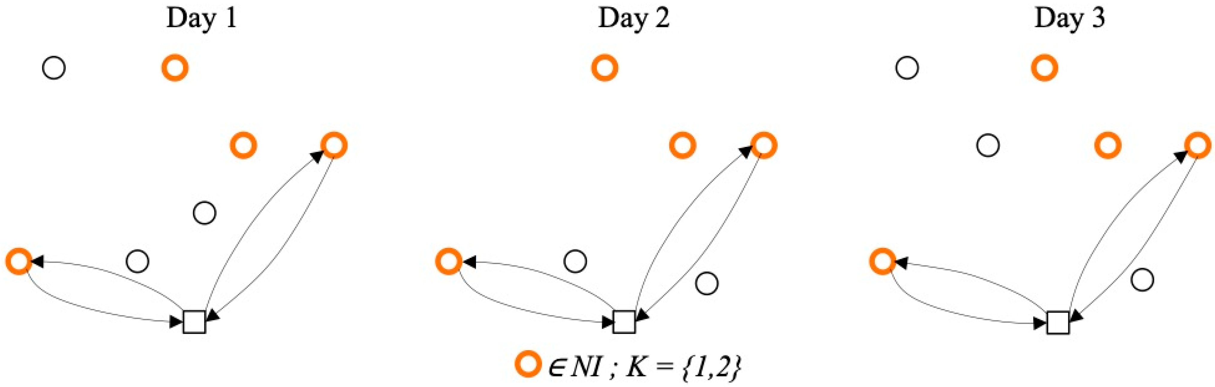
  • wid: Requested service by customer i for day d. This parameter takes a value of 1, indicating that customer i has a demand on day d.
  • tij: Travel time from node to node j.
  • sid: Service time of customer i for day d.
Decision variables:
  • x i j k d = 1   if the vehicle   k   visits the customer   j   after visiting customer   i   for the day   d 0   Otherwise .
  • y i k d = 1   if the customer   i   is served by the vehicle   k   for the day   d 0   Otherwise .
  • a i d = A r r i v a l   t i m e   o f   c u s t o m e r s i on the day d.
Objective function and constraints
min d D k K i , j A t i j x i j k d
y 0 k d = 1               k K ,   d D
a 0 d = 1               d D
k K y i k d = w i d             i N ,   d D
i N q i d y i k d Q             i N , d D , k K
i V x i j k d = y j k d             j N , k K , d D
i V x j i k d = y j k d             j N , k K , d D
w i d α + w i d β 2 = y i k d α y i k d β           d α , d β D ,   i N , k K , d α d β
w i d α + w i d β 2 = y i k d β y i k d α           d α , d β D ,   i N , k K , d α d β
a i d + x i j k d s i d + t i j 1 x i j k d T a j d           i , j A : j 1 , k K , d D
a i d + x i j k d s i d + t i j + 1 x i j k d T a j d           i , j A : j 1 , k K , d D
a i d + w i d s i d + t i 0 0           i N , d D
a i d + w i d s i d + t i 0 T w i d             i N , d D
a i d α a i d β L + T 2 w i d α w i d β           d α , d β D : d α d β , i N
a i d β a i d α L + T 2 w i d α w i d β           d α , d β D : d α d β , i N
x i j k d 0 , 1           i , j V ,   k K , d D
y i k d 0 , 1           i N , k K , d D
a i d 0           i N , d D
The objective function of Model (1) is to minimize the vehicle travel time. This metric differs from the total duration of the route by not considering the time dedicated to customer service. Constraints (2) ensure that each driver must start the route at the depot and travel to the first customer. Constraints (3) imply that every driver must serve at least one customer each day of the planning horizon. Constraints (3) require that all routes start simultaneously (time 0 as a reference). Constraints (4) determine that if a customer requires service on a particular day, then this will be fulfilled. Constraints (5) imply that the total amount of products demanded by customers served on each route must be at most the vehicle’s capacity. Constraints (6) and (7) determine that each customer has a single predecessor and successor on the route. Constraints (8) and (9) control that each customer requiring multiple services during the planning horizon is served by the same driver.
Constraints (10) and (11) determine the arrival times for each customer on each day of the planning horizon and imply that the driver must immediately move to the next node after serving a customer. Constraints (12) and (13) ensure that the duration of any route is, at most, the maximum operating time. Constraints (14) and (15) determine that every customer requesting service on multiple days must be served with a maximum difference of L units of time between different days of the planning horizon. Therefore, it is necessary to determine the service schedule for each customer on each day of the planning horizon. Constraints (16) and (17) limit the domain of the decision variables x i j k d and y i k d to binary values, and constraint (18) ensures non-negativity in the values of a i d .

3.2. Proposed Solution Method

This section describes the proposed heuristic method to solve the ConVRPms. The first section describes the main characteristics and general algorithmic structure. In subsequent sections, each of the components is described in detail.

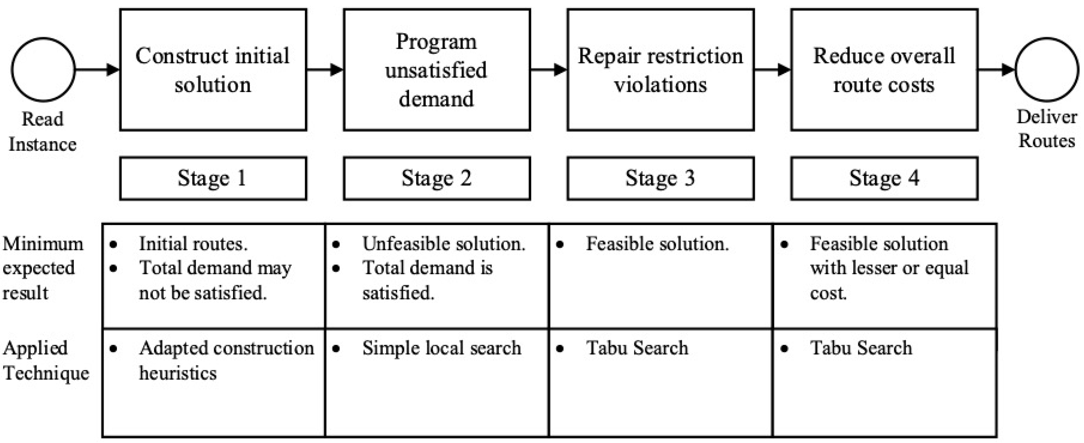
3.2.1. Description of the Proposed Algorithm

The proposed tabu search-based repair and improvement (TSRI) algorithm is a deterministic heuristic designed to solve the problem of consistent vehicle routing with minimum service (ConVRPms). The TSRI algorithm integrates construction heuristics and procedures based on a tabu search metaheuristic [26] to produce high-quality solutions within short computing times. The theoretical complexity of the proposed approach is O(n3) because local searches based on 2-opt moves indicate that the computing time of the algorithm grows cubically with the input size. However, the architecture of the former allows high-quality solutions to be obtained within short computing times.
The algorithm has a sequential structure of four stages focused on constructing an initial solution, obtaining a complete solution, addressing infeasible solutions, and reducing the total cost of the routes. Figure 1 shows a representative process diagram of the TSRI algorithm, indicating the applied techniques and the minimum expected results for each stage.
Let H e u r i s t i c be the algorithm used, λ be the value of the respective heuristics-controlled parameter, n R e p be the limit of the number of iterations of the repair process, and n M e j be the number of iterations in the improvement process. The pseudocode of the TSRI algorithm is presented below:
Pseudocode 1. Proposed TSRI Algorithm
Procedure TSRI ( I n s t a n c e , H e u r i s t i c , λ , n R e p , n M e j )
         S Construct_solution( I n s t a n c e , H e u r i s t i c , λ )
        If  d e m a n d   i s   n o t   c o m p l e t e l y   s a t i s f i e d  then
               S Schedule_unsatisfied_demand( S )
        If  s   i s   n o t   f e a s i b l e   then
                  S Repair_solution( n R e p , S )
        If  s   i s   f e a s i b l e   then
             S Improve_solution( n M e j , S )
                Output:  S     Feasible Solution
        Else
                Output:   S     Infeasible Solution
Return S

3.2.2. Stage 1: Constructing an Initial Solution

The first stage of the TSRI algorithm consists of constructing an initial solution. For the construction of the VRP, adaptations of classic heuristics, the savings heuristic of [27], and two insertion heuristics [28], are used. Ref. [28] stated that the savings heuristic produces higher-quality solutions for the VRP. On the other hand, Ref. [29] highlighted the effectiveness of the best insertion heuristic to generate feasible and low-cost solutions.

Savings Heuristic

The savings method of [27] was the first heuristic adapted to generate the initial solution. This adaptation is based on the version proposed by [9] to generate feasible initial solutions for the ConVRP. This adaptation presents substantial differences because the ConVRPms approach does not allow for unlimited vehicles.
The fundamental idea of the savings heuristic is constructing a solution using the repeated union of routes to obtain the maximum objective function reduction for each iteration. In this case, the objective function is the total travel time of the vehicles. The first procedure generates an initial route for each customer daily. The same vehicle is assigned to all the routes of the same customer to satisfy the consistency constraint of the DC driver. Then, for each iteration, the potential route junctions for each pair of vehicles are modeled, and the respective savings are calculated. Four different union types, referred to as movements, have been proposed.
Let k and l be two vehicles that serve at least one customer for the current solution. α k d and α l d are the first customers served by the respective vehicles on day d , and ω k d and ω l d are the last served customers. The four movements used to join the routes of these two vehicles are as follows:
  • The route of vehicle l is inserted after the route of vehicle k
    [ α k d , ,   ω k d ] _ α l d , ,   ω l d _ α k d , ,   ω k d , α l d , ,   ω l d _ d D :   y 0 k d = 1
    Route k of the day d Route l of the day d New route of day d
  • The route of vehicle l is inserted before the route of vehicle k
    α k d , ,   ω k d _ α l d , ,   ω l d _ α l d , ,   ω l d , α k d , ,   ω k d _ d D :   y 0 k d = 1
    Route k of the day d Route l of the day d New route of day d
  • The inverse route of vehicle l is inserted after the route of vehicle k
    α k d , ,   ω k d _ ω l d , ,   α l d _ α k d , ,   ω k d , ω l d , ,   α l d _ d D :   y 0 k d = 1
    Route k of the day d Inverse Route l of the day d New route of day d
  • The route of vehicle l is inserted after the inverse route of vehicle k
    ω k d , ,   α k d _ α l d , ,   ω l d _ ω k d , ,   α k d , α l d , ,   ω l d _ d D :   y 0 k d = 1
    Inverse Route k of the day d Route l of the day d New route of day d
Then, the total net savings are calculated from the union of the routes of k and l by means of the respective move m according to (19):
s k l d m = λ A t ω k d 0 + t α l d 0 t ω k d α l d   i f   m = 1   y 0 k d = y 0 l d = 1 λ A t α k d 0 + t ω l d 0 t α k d ω l d   i f   m = 2   y 0 k d = y 0 l d = 1 λ A t ω k d 0 + t ω l d 0 t ω k d ω l d   i f   m = 3   y 0 k d = y 0 l d = 1 λ A t α k d 0 + t α l d 0 t α k d α l d   i f   m = 4   y 0 k d = y 0 l d = 1 0             O t h e r w i s e
The total net savings for the planning horizon are as follows:
S k l m = d D s k l d m
λ A is a parameter that controls the relative weight between savings and costs incurred in the union of two routes. For values greater than 1, the connections between nodes farthest from the depot are prioritized. With values lower than 1, the connections between customers closest to the depot are prioritized.
Each joint is identified by the pair of vehicles involved and the type of movement. The joints are arranged in decreasing order of total savings S k l m , and then, the feasibility of the joints is evaluated in an orderly manner. The feasibility of each connection is evaluated by calculating the total load and route duration and the arrival time for each served customer on each day of the planning horizon. Suppose that all routes of vehicle k must transport a load less than the maximum capacity Q , have a shorter duration than T , and serve every customer with a difference of at most L units of time between arrival times. In that case, the union is feasible, and the solution is updated. In the opposite case, the subsequent union on the list is evaluated.
The initial heuristic ends once it is impossible to perform another union feasibly or if it is possible to serve all customers with K vehicles. Considering that the heuristic starts with | N | vehicles, it is possible that the number of routes cannot be served with the available fleet. In this case, the routes of daily deliveries are eliminated. If the number of vehicles used continues to exceed the available fleet, the routes that serve the fewest customers are removed. Unserved customers are addressed in stage 2 of the TSRI algorithm.

Parallel Insertion Heuristic

Insertion heuristics consist of the construction of an initial solution through the repeated inclusion of one customer at a time. In the present work, two variants of the insertion heuristic are proposed. The parallel insertion heuristic differs from its sequential alternative by evaluating the insertion of each remaining customer in the routes of all available vehicles. The heuristic of parallel insertion includes two processes: the initialization of the routes and the insertion of customers. All routes are initialized prior to the insertion of customers to satisfy the empty route constraint (14) and build potentially more economical solutions by generating dispersed initial routes, thus avoiding the inclusion of the most expensive arcs. Therefore, | K | nodes belonging to the set of N I customers that demand service every day and that maximize the total distance between them and their distances to the depot are selected. Figure 2 shows an example of an insertion heuristic.
After the routes’ initialization, the remaining customers’ insertion process begins. Given that the ConVRP is a multiday problem, all position configurations in which each customer can be inserted are evaluated. The consistency constraint of the DC driver limits the search space by defining the insertion operator consisting of the driver.
The insertion operator consisting of a DC driver includes the selection of a customer j belonging to the set of remaining nodes R N and its insertion in the route of a vehicle k on each day d that the customer j demands service ( d D : w j d = 1 ). There are multiple position configurations for each remaining customer to be inserted. The position is defined using the subsequent nodes p k d that would be served immediately after j in the routes of vehicle k for each day d , in which customer j requests service as a reference.
Once all the potential DC insertion operations are identified, the total cost of each operation is calculated. Let p k d be the node after the insertion of j in the route of vehicle k on day d . s k d is the node served before p k d in the current solution. The net cost of the insertion c j d p k d of customer j on day d between nodes s k d and p k d is defined by the following expression (21):
c j d p k d   = λ P t s k d j + t j p k d t s k d p k d ,   i f   w j d = 1 0 ,   O t h e r w i s e       d D
The total cost associated with the insertion is the sum of its daily net costs.
c j , p k 1 , p k 2 , , p k D = d D c j d p k d
The parameter λ P controls the relative weight between the cost and the savings generated from the insertion. For values of λ P greater than 1, insertions between nearby nodes are prioritized, whereas for values of λ P less than 1, insertions between distant nodes are prioritized.
The insertions are arranged in ascending order concerning total cost, and their feasibility is evaluated. The evaluation is carried out in the same way as in the savings heuristic. It is carried out upon identifying a feasible insertion, and another iteration of the insertion process is executed. The heuristic ends when all customers have been included or if it is impossible to include an additional customer without violating any constraint. Figure 3 shows an example of an insertion operator for DC. For the insertion operator, a customer is removed from route A and inserted into route B at the best location, minimizing the total travel cost (Figure 3).

Sequential Insertion Heuristic

There are specific differences between the sequential insertion heuristic and its parallel alternative. The main difference is the insertion process; only the DC insertions in the routes of a single vehicle are modeled and evaluated. As a result, a procedure is included to select the vehicle for sequential insertion.
The initialization of the routes is carried out in the same way as in the parallel insertion heuristic. The vehicle selection procedure is applied after the initialization of the routes, and on each occasion, it is impossible to insert another customer in the routes of the current vehicle. The criterion used to select the vehicle for the subsequent insertion is the minimization of the total distance between the node initially served by the vehicle and the set of customers not included in the current routes R N . Let R K be the set of vehicles not previously selected; vehicle k can be identified by evaluating the following expression for each k R K .
min k RK j N ( y j k d i R N d D w i d t j i )
In the insertion process, only the DC insertions in the routes of k are modeled and evaluated. Once all the insertion operations for vehicle k have been identified, the total cost for each operation is calculated. Analogous to calculating the total cost with the parallel insertion heuristic, a parameter λ S is incorporated to control the relative weight between the cost of the new arcs and the savings generated with each operation.
Let p k d be the node after the insertion of j on the route of the selected vehicle k on d . s k d is the node served before p k d in the current solution. The net cost of the insertion c j d p k ^ d of customer j on day d between nodes s k d and p k d is given by
c j d p k ^ d = λ S t s k ^ d j + t j p k ^ d t _ s k ^ d p k ^ d 0 ,     e . o . c .         d D
The total cost of insertion in the planning horizon is calculated via the following equation:
C j , p k ^ 1 , p k ^ 2 , , p k ^ | D | = d D c j d p k ^ d
After the operation and ordering costs are calculated according to the total cost, the operations are evaluated to search for a feasible insertion. When it is impossible to add another customer to the routes of the currently selected vehicle k , the vehicle selection procedure is applied. The sequential insertion heuristic ends when all customers have been included in the routes or if there are no additional vehicles to select ( R K = Ø ).

3.2.3. Stage 2: Scheduling Unsatisfied Demands

Stage 2 of the TSRI algorithm consists of a simple local search process that aims to schedule the remaining customers in the routes of an incomplete initial solution. For each iteration of the completion process, a new solution s n is produced that better satisfies the individual demands of a customer in its routes than the previous solution s n 1 . Indeed, given that the neighborhood N C ( s n 1 ) of s n 1 exclusively includes all the DC insertion operations of a customer not served in the solution s n 1 . Note that all the operators seek the best improvement of the following current objective function:
N C s = N i n s e r t i o n ( s )
The objective function of the local search has been designed to minimize the number of violated constraints and, in the background, the value of the objective function of the problem. Let σ l o a d s be the number of routes whose load exceeds the vehicle’s capacity in solution s , σ m i n s be the number of empty routes, σ d u r s be the number of routes whose duration exceeds the time limit, and σ a t c s be the number of customers whose service schedules are inconsistent. The following expression defines the objective function f C s of the local search.
min s N C s n f C s = σ l o a d s + σ m i n s + σ d u r s + σ a t c s + i , j , k , d x i j k d s t i j t i j
Let s 0 be the initial solution; the completion process is represented by the following pseudocode:
Pseudocode 2. Proposed Completion Process Algorithm
Procedure completion (schedule with unsatisfied demand s 0 )
         R N Unsatisfied customers in s 0
        For  n 1 : R N              s n Local_search( f C s , N C s n 1 ,   s n 1 )
Return Complete solution: s n

3.2.4. Stage 3: Repairing the Solution

The third stage of the TSRI algorithm consists of a process based on the tabu search metaheuristic, whose objective is to obtain a feasible solution through the progressive reduction of the number and type of violations. The repair process comprises three subprocesses: repairing empty routes or routes with excessive loads, repairing routes with excessive duration, and repairing routes with inconsistent arrival times. Each subprocess mentioned above has a neighborhood structure and a distinctive objective function.
The resulting solution in each iteration of the repair process is recorded in the tabu list, prohibiting the selection of the same solution again in a subsequent iteration. Let N ( s n ) be the neighborhood of s n and T L n be the set of solutions belonging to the tabu list in iteration n of the repair process. The allowed neighborhood N ^ ( s n )   is the subset of solutions that can be selected such that N ^ ( s n ) = N ( s n )   \   T L n . The tabu list is restarted at the end of each repair thread.

Repairing Empty or Overloaded Routes

This subprocess is applied if a load of at least one route exceeds the vehicle’s capacity or if at least one driver serves no customer on any given day. The DC repositioning and inter-route exchange operators define the neighborhood structure of the local search in this subprocess. Representations of these operations are presented in Figure 4.
N R 1 s = N r e l o c a t e s N i n t e r c h a n g e ( s )    
The objective function of the local search penalizes solutions with load and minimum service violations. Let B i g M be a very large number ( B i g M > 4 · | K | · | D | + 2 · | N | | ); then, the objective function of the local search in the subprocess of repairing empty routes or with excessive loads f R 1 s is presented below:
min s N ^ R 1 ( s n ) f R 1 s = B i g M ( σ l o a d s + σ m s s ) + σ d u r s + σ a t c s + i j k d x i j k d s t i j t i j
The subprocess ends when every route serves at least one customer and when the transported load is less than or equal to the capacity of vehicle σ l o a d s n + σ m s s n = 0 .

Repair Routes with Excessive Duration

The second repair subprocess is applied if at least one route violates the maximum duration constraint. The structure of the neighborhood has been defined through the DC repositioning of the 2-opt intraroute and inter-route operators.
N R 2 s = N r e l o c a t i o n s N s i n g l e 2 o p t s N e x c h a n g e ( s )  
The initial solution must respect the maximum load and minimum service constraints, and the violation of these constraints is penalized in the objective function, thus avoiding going backward in the general objective of the repair process. Let d u r a t i o n k d s be the duration of the route served by driver k on day d in solution s ; then, the objective function of the second subprocess is defined below.
min s N ^ R 2 ( s n ) f R 2 s = B i g M ( σ l o a d s + σ m s s ) + σ a t c s + σ d u r s 1 + k d d u r a t i o n k d s 2 T 2
The objective function prioritizes the solutions that minimize the number of duration violations and ATC violations. The function accompanying σ d u r s always returns a value between 1 and 2. It is used to avoid the reduction of the duration of some routes at the expense of the increase in others with already excessive durations. The subprocess ends when no route serves any customer, carries a load greater than Q , or has a duration greater than T σ d u r s n + σ l o a d s n + σ m i n s n = 0 .

Repairing Inconsistent Arrival Times

This subprocess is applied if all the constraints of the solution are satisfied except for the consistency of arrival times. The structure of the neighborhood has been defined through DC repositioning, inter-route interchange, and 2-opt multiroute operators. Please see Figure 5.
N R 3 s = N r e l o c a t i o n s N m u l t i 2 o p t s N e x c h a n g e ( s )
The objective function is designed to progressively reduce the number of ATC violations until a feasible solution is achieved.
min s N ^ R 3 ( s n ) f R 3 s = B i g M ( σ l o a d s + σ m s s + σ d u r s ) + σ a t c s + i a t c i s 2 T 2
The sum at the end of the expression prioritizes the selection of solutions whose customers are served with highly consistent schedules and penalizes solutions with irregular schedules ( a t c i s > L > 0 ). Let n R e p be the limit of iterations of the repair process. The pseudocode of the complete repair process is presented below:
Pseudocode 3. Proposed repair procedure
Procedure Repair Procedure (Non-feasible solution, s 0 , n R e p )
         n 0
         T L 0   s 0
        While  σ l o a d s + σ m s s > 0     Λ ( n < n R e p ) do
                   n   n + 1
                   s n   ← Local_search( f R 1 s , N R 1 ( s n 1 ) , T L n 1 )
                 T L n T L n 1 s n
         T L n s n
        While  σ l o a d s + σ m s s + σ d u r s > 0     Λ ( n < n R e p ) do
                   n   n + 1
                   s n   ← Local_search( f R 2 s , N R 2 ( s n 1 ) , T L n 1 )
                 T L n T L n 1 s n
         T L n s n
        While  σ l o a d s + σ m s s + σ d u r s + σ a t c s > 0     Λ ( n < n R e p ) do
                   n   n + 1
                   s n   ← Local_search( f R 3 s , N R 3 ( s n 1 ) , T L n 1 )
                 T L n T L n 1 s n
         T L n s n
        Finalize Repair process
        If  ( σ l o a d s + σ m s s + σ d u r s + σ a t c s = 0 )   then
                Output: Feasible solution: s n
        Else
                Output: Infeasible solution: s n
        Return s n  
The repairing procedure is a tabu search-based iterative process designed to reduce constraint violations in an initially infeasible solution, progressively. Following the structure of the TSRI algorithm, the procedure is divided into three sequential subprocesses, each addressing a specific type of violation through a dedicated local search. Tabu search principles guide these local searches and operate over well-defined neighborhood structures. A tabu list T L is used in each subprocess to record recently visited solutions and avoid cycling; this list is reset between subprocesses to encourage exploration of distinct regions of the solution space.
  • The neighborhood NR1 is defined by DC repositioning and inter-route exchange operators and is focused on eliminating empty or overloaded routes.
  • The neighborhood NR2 addresses violations related to excessive route durations, incorporating DC repositioning, 2-opt intraroute operators, and inter-route operators.
  • The neighborhood NR3 is designed to correct inconsistencies in customer arrival times and includes DC repositioning, inter-route exchange, and 2-opt multiroute operators.
In each stage, the local search explores the non-tabu neighborhood to find the best admissible solution, either by reducing the number of violations or increasing the overall cost. At the end of the process, the best solution identified across all stages is returned—ideally, a fully feasible solution ready for subsequent improvement.

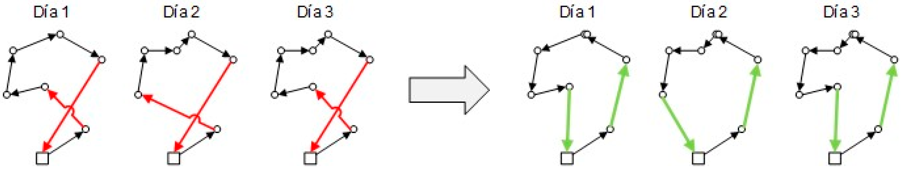
3.2.5. Stage 4: Improving the Solution

The last stage of the TSRI algorithm consists of an improvement process based on the tabu search metaheuristic, whose objective is to reduce the total displacement time of the final solution. An approach has been designed to efficiently exploit the local search in the space of feasible solutions and guide the search to subspaces of higher-quality solutions through trajectories in infeasible solutions. This approach is applied through the objective function of local search f M s .
Let f z s be a function equivalent to the objective function of the original mathematical model (1) and let s be the feasible solution with the lowest value of f z s found thus far. Then, z s u b o p t is a binary auxiliary variable that indicates whether the solution s has a value of f z s equal to or greater than f z s b e s t .
f z s = i j k d x i j k d s t i j
z s u b o p t s , s b e s t = 1 ,   i f   f z s f z s b e s t 0 ,   i f   f z s < f z s b e s t
f i n f s = σ l o a d s + σ m s s + σ d u r s 1 + k d d u r a t i o n k d s 2 T 2 + σ a t c s ( 1 + i a t c i s 2 T 2 )
The objective function f M s of the local search is presented below:
min s N ^ M f M s = f z s + B i g M f i n f s + B i g M 2 z s u b o p t ( s , s b e s t )  
The structure of the neighborhood in the improvement process is defined by the DC repositioning operators: 2-opt intraroute and inter-route interchange.
N M s = N r e l o c a t i o n s N s i n g l e 2 o p t N e x c h a n g e
Pseudocode 4. Proposed Improving Procedure
Procedure Improving Procedure (Feasible Solution, s 0 , n M e j )
         n 0
         s b e s t   s 0
         T L 0   s 0
        While  n < n M e j  do
                   n   n + 1
                   s n   ← Local_search( f M s , f z s b e s t ,   N M ( s n 1 ) , T L n 1 )
                   If f M s n < f z s b e s t    then
                   s b e s t   s n
         T L n T L n 1 s n
Output: Feasible solution: s b e s t
Return s n
The final stage of the TSRI algorithm corresponds to improving a feasible solution through a tabu search-based local search. Unlike the previous repair stage, which focuses on constraint satisfaction, this phase assumes a feasible input solution and aims to minimize travel time across all routes. The improvement procedure uses the same metaheuristic structure but shifts the objective function toward solution cost rather than feasibility.
The search is conducted within a neighborhood N M , defined by DC repositioning, 2-opt intraroute, and inter-route exchange operators. These moves are applied iteratively to explore increasingly better configurations of the existing solution. A tabu list T L is maintained throughout the process to prevent revisiting recently explored solutions. The algorithm is executed for a fixed number of iterations, defined by the parameter n M e j .

4. Computational Experiments

4.1. Experimental Environment and Hardware

The TSRI algorithm was implemented in the Julia programming language (version 1.6.1) through Visual Studio (version 1.58.2). The experiments were carried out on a computer with a Windows 10 Home 64-bit operating system, 16 gigabytes of RAM, an Intel Core i5-8300H @ 2.3 GHz quad-core processor, and eight threads. For study purposes, only one thread of the processor was used.
As a reference, the CPUmark score of this processor is 7543. In contrast, the processor used by Barros et al. [3] (Intel Xeon E5-2660 v2 @ 2.20 GHz) to solve the test instances through CPLEX has a CPUmark score of 10,409, and ten threads of the processor are used in parallel.

4.2. ConVRPM Test Instances

The instances of the problem applied in the experiments correspond to the structured instances from [3], which were synthetically designed to analyze the performance of the model against changes in the size of the instance, the geographical distribution of customers, the location of the depot, and the required level of consistency in arrival times. The set includes 33 instances whose sizes N vary between 10, 15, and 20 customers, and the geographical distribution of these customers can be uniform or in agglomerations. The depot can be located in the center or corner of the plane, and the value of the parameter L , which determines the consistency in the required arrival times, can take values of 1, 3, and T, the latter corresponding to the total relaxation of the ATC constraint.
Each instance has a planning horizon D of three days and a fleet of two or three K vehicles with a homogeneous capacity Q of fifteen units. The individual demand of each customer q i d varies uniformly between zero and three units each day, and the service time s i d   varies between zero and two time units. The locations of the customers and the depot were determined within a square plane of dimensions 10 × 10 units in length. The parameter t i j   was determined by calculating the Euclidean distance between each pair of nodes and then transforming the distance into units of time with a ratio of 1:1.

4.3. First Experiment

The first experiment consisted of the execution of the first two stages of the TSRI algorithm—construction and completion—to identify the values of the parameters λ A , λ P , and λ s that produce a more significant proportion of feasible solutions, and to analyze the efficiency of the first two stages of the algorithm in obtaining feasible solutions for different subsets of the instances, which were segmented according to the consistency in arrival times needed.
For each adapted constructive heuristic (savings, parallel insertion, and sequential insertion), 41 scenarios in which the value of the corresponding controlled parameter λ varied were defined. An initial solution was built and completed for each of the 33 instances in each scenario. The values of λ A , λ P , and λ s varied between 0.00 and 2.00 at regular intervals of 0.05.
In the first section, the results of the first experiment are presented. First, the populations of solutions generated in each scenario were analyzed, and the λ values that produced the best initial solutions with each constructive heuristic were identified. Then, the proportion of feasible solutions of the scenarios with the best-observed performance was analyzed by segmenting the instances according to the consistency in the required arrival times.
Figure 6 contains a set of three scatter plots in which the proportion of feasible solutions and the average lower-bound BKS of the population of feasible solutions produced in each scenario of the first experiment are shown.
The number of feasible solutions and their quality are sensitive to the variation in the value of the corresponding parameter λ of each constructed heuristic, and no scenario results in a proportion of feasible solutions of 100%.
The maximum proportion of feasible solutions observed when applying the savings heuristic was 60.6 percent, equivalent to 20 feasible solutions of 33 total solutions when λ A equaled 1.05. The average lower-bound BKS of the feasible solutions in this scenario was 7.8%. The maximum proportion of feasible solutions observed in the scenarios in which the parallel insertion heuristic was applied was 66.7%, with λ P values equal to 0.65, 0.70, and 1.85. The average BKS observed in these three scenarios was 8.4%, with λ P equal to 0.65. Finally, the maximum proportion of feasible solutions observed when applying the sequential insertion heuristic was 69.7 percent, obtained with values of λ S equal to 0.85, 0.95, 1.40, 1.45, and 1.50. The lowest average BKS limit observed in these scenarios was 24.0%, which was obtained with λ S equal to 0.85.
Figure 7 shows the proportions of feasible solutions of the scenarios with λ A , λ P , and λ s equal to 1.05, 0.65, and 0.85, respectively, in different subsets of the test instances, which were segmented according to the level of requirement of the ATC constraint.
The three heuristics produced initial feasible solutions in one third of the instances, with L equal to 1. The proportion of feasible solutions increased considerably for the instances with values of L equal to 3 or T . However, the construction heuristics and the completion process needed to be revised to obtain feasible solutions for all instances, even for the segment with the ATC constraint, which was relaxed. Finally, each solution produced in the first experiment was constructed and completed in an average of 0.20 s, without a significant difference when different heuristics were used.

4.4. Second Experiment

The second experiment consists of executing the four stages of the TSRI algorithm in the set of test instances in different scenarios. The observed values of λ that produced the highest proportion of feasible solutions and the lowest average lower-bound BKS in the first experiment were used. The parameter n R e p , which determines the limit number of iterations of the repair process, was set at 250. In each scenario, one of the different variants of the TSRI was used, and the value of the parameter n M e j equaled zero, ten, or fifty, which determines the number of iterations of the improvement process.
Let V a r be the set of variants { 1 = T S R I A , 2 = T S R I P , 3 = T S R I S } and M e j be the set of explored values of n M e j = { 0 , 10 , 50 } , whose combination defines the scenarios of the second experiment. Let E be the set of stages of the TSRI algorithm { 1 = C o n s t r u c t i o n ,   2 = C o m p l e t i o n ,   3 = R e p a i r ,   4 = I m p r o v e m e n t } and I be the set of test instances { 1 , 2 , 32 , 33 } . The following set of variables was measured for each solution at the end of each stage of the TSRI algorithm in each scenario of the second experiment.
  • Feasibility of the solution: F a c t i e v n { 0 , 1 }
  • Completeness of the solution: C o m p i e v n { 0 , 1 }
  • Cost value of the solution: z i e v n = f z ( s )
  • Total computing time: T . C P U i e v n
Then, for each solution, the relative bound of the cost z i e v n was calculated concerning the highest lower bound obtained with CPLEX ( L B n ) and its relative bound concerning the most economically feasible solution known for the corresponding instance ( B K S n ).
G A P i e v n L B = z i e v n L B i L B i 100 %         i I , e E , v V a r ,   n M e j
G a p i e v n B K S = z i e v n B K S i B K S i 100 %         i I , e E , v V a r , n M e j
The values of L B n and B K S n are provided in the comparative tables of the final solutions (see Appendix Section).
The statistical parameters used to analyze the performance of the algorithm in the solution of the set of test instances are calculated from the following expressions:
A v g L B e v n = i I G A P i e v n L B F a c t i e v n i I F a c t i e v n         e E , v V a r , n M e j
A v g B K S e v n = i I G a p i e v n B K S F a c t i e v n i I F a c t i e v n         e E , v V a r , n M e j
A v g T . C P U e v n = i I T . C P U i e v n F a c t i e v n i I F a c t i e v n         e E , v V a r , n M e j
% F a c t e v n = i I F a c t i e v n i I 1 100 %       e E , v V a r , n M e j
% F a c t B K S e v n = i I F a c t i e v n     i I : ( z i e v n B K S i ) i I 1 100 %       e E , v V a r , n M e j
% N o F a c t B K S e v n = i I ( C o m p i e v n F a c t i e v n )     i I 1 100 %       e E , v V a r , n M e j
( D e s v B K S e v n ) 2 = i I ( G a p i e v n B K S A v g B K S e v n   ) 2 F a c t i e v n i I F a c t i e v n       e E , v V a r , n M e j
Next, the results of the second experiment are presented. First, the final solutions obtained for each experimental scenario were described and analyzed. The individual contribution of each stage of the TSRI algorithm for the set of instances was analyzed. The performance of the TSRI algorithm was compared with the experimental results reported by [3], and the performance of the different variants of the TSRI algorithm in different segments of the set of instances was compared. Finally, the best new solutions discovered for structured instances were identified.
Table 1 shows a set of statistical parameters of the population of final solutions obtained in each scenario of the second experiment.
All the final solutions obtained with the P and S variants of the TSRI algorithm were feasible. In all the scenarios corresponding to variant A, the proportion of feasible solutions was 97.0%, which was equivalent to one infeasible solution of thirty-three total solutions. The proportion of feasible solutions with a cost z less than or equal to the cost of the best-known BKS solution was greater than 50 percent in all scenarios with fifty iterations of the improvement process and ten iterations when applying variant A of the TSRI algorithm.
The solutions generated in the scenarios with n M e j equal to 50 or 10 had a lower average value of G A P i e v n L B and G a p i e v n B K S and a lower standard deviation of B K S e v n ( D e s v B K S e v n )   than the solutions obtained in scenarios with a lower number of iterations. The average computing time with n M e j = 50 approximately quintupled the average computing time with n M e j = 10 , and the latter approximately doubled the average computing time with zero iterations of the improvement process. The average computing times required to obtain a feasible solution with variants A, P, and S of the TSRI algorithm were 12.94, 9.38, and 10.55 s, respectively. When comparing the three variants in the scenarios with n M e j   equal to 50, the TSRI-P variant produced a population of 100% feasible solutions with the lowest average values of G A P i e v n L B , G a p i e v n B K S , and total computing time.
Table 2 shows the costs (z) and total computing time (T.CPU) of the solutions generated with the different variants of the TSRI algorithm and the solutions obtained via CPLEX in Barros et al. (2020) [3] for instances 6, 8, and 9.
At least one feasible solution was discovered with a cost z lower than the BKS for each instance. The best solutions were obtained with the P variant of the TSRI algorithm. Instances 6, 8, and 9 belong to the set of instances with 20 customers and with a maximum demand in the arrival times ( L equal to 1). Appendix section shows the graphical representation of the new best solutions discovered and the solutions obtained via CPLEX in Barros et al. (2020) [3] for instances 6, 8, and 9, respectively.
Figure 8 shows the A v g L B e v n , A v g B K S e v n , and average computing time T.CPU of the final solutions generated with each variant of the TSRI algorithm and the solutions generated by the CPLEX branch-and-cut approach in Barros et al. (2020) [3].
The feasible solutions produced with the three variants of the TSRI algorithm were observed to have a higher average A v g B K S e v n than those obtained with CPLEX. On average, the solutions generated with the TSRI-P variant had a cost z 2.1 percent higher than the BKS cost of the best-known solutions obtained through CPLEX. The average BKS limit is slightly lower with the TSRI-A variant; however, not all solutions were feasible with this variant. A significant difference was observed between the average computing time of the TSRI algorithm and the average observed time of the exact method. The TSRI-P variant with 50 iterations of the improvement process took 101.6 s on average to deliver each final solution, in contrast to the 1535.9 s of CPLEX. Figure 9 shows the average computing times of the TSRI-P and CPLEX B and C variants in different instances, segmented according to the number of customers or the consistency in arrival times needed.
The average computing time observed with CPLEX was 12 s greater than that of the TSRI-P in the instances with ten customers. This difference increased to 1130 s in the instances with fifteen customers and 2898 s with twenty customers. When segmenting the instances according to the value of the parameter L , it is possible to observe that both methods took longer to compute the solutions with L equal to 1. The average T.CPU observed with the TSRI-P algorithm was lower for the instances with L equal to 3. In contrast, CPLEX took less time to compute the solutions with a fully relaxed ATC constraint ( L equal to T ). Figure 10 shows three statistics of the solutions generated with the TSRI-P variant and n M e j = 50 at the end of each of the four stages of the TSRI algorithm: construction, completion, repair, and improvement.
At the end of Stage 1 of the TSRI algorithm, feasible solutions were obtained for a fraction of the total test instances. At the end of the second stage, all the solutions were feasible or infeasible. At the end of the third stage, all the solutions were feasible. At the end of the fourth and final stages, the solutions had a lower average BKS than those obtained at the end of the third stage (repair stage). Finally, the feasible solutions obtained at the end of the fourth and final stages had a lower A v g B K S e v n than those obtained at the end of the repair stage.
Figure 11 shows the A v g B K S e v n of the final solutions for different subsets of the test instances, segmented according to the size of the instance, the distribution of customers, the location of the depot, or the consistency in arrival times needed. The solutions corresponding to instance 3 (15UC1) were excluded because the TSRI variant produced an infeasible solution.
The TSRI—A variant (savings heuristic) generated solutions of higher quality than the other two variants in the instances with the depot located in the center of the plane and the instances with a very tight or relaxed ATC constraint ( L     { 1 , T } ). When segmenting according to the customers’ geographical distribution, the P variant (parallel insertion) performed better than the other two variants did in instances with uniformly distributed customers and customers distributed in clusters. It also produced more economical solutions in instances with a moderate ATC requirement ( L = 3 ). Finally, the S variant (sequential insertion) performs better in instances with 15 or 20 customers and where the depot is located in the plane’s corner.

5. Discussion of the Results

The experimental results demonstrated the competitiveness of the TSRI algorithm over CPLEX in terms of the solution of the structured instances of the ConVRPms, generating high-quality solutions in a computing time considerably less than those reported in the literature. When comparing the solutions produced with the TSRI-P variant, the average cost was 2.1 percent higher than those generated with CPLEX. It was computed in a time equivalent to 6.6% of the average value observed with the exact method. In addition, it produced higher-quality solutions in some of the largest and time-restricted instances.
It is important to consider the disparity in the hardware used to process the solutions in the present investigation and the study carried out by [3]. It is expected that more iterations of the repair and improvement processes could be processed in less computing time with comparable resources. The main competitive advantage of the proposed method over the exact method is its speed, which is reflected in the observed computing times. The difference in the performance of both methods increased with increasing problem size and arrival time demand. In contrast, the inability to evaluate the quality of the solutions is a weakness of many heuristic methods, including the TSRI algorithm. Compared with the costs reported by [3], some solutions were up to 5.5% less expensive, and others were up to 23.6% more expensive.
Each variant of the TSRI algorithm performed better than its alternatives in terms of the quality of solutions generated in different segments of the set of instances. In conjunction with the relatively low computing times of the first two stages (construction and remaining demand schedule) compared with those of the last two stages (repair and improvement), the evaluation of multiple initial candidate solutions could considerably improve the quality of the final solution at the expense of a marginal increase in computing time. Other methodologies proposed in the literature for the solution of VRPs with consistency considerations incorporate the evaluation of multiple initial solutions prior to the metaheuristic components. The stages of the TSRI algorithm were effective in achieving their objectives. The adapted constructive heuristics could generate feasible solutions in more than half of the instances, the repair process made almost all programs with violated constraints feasible, and the improvement process considerably reduced the cost of the routes. Another relevant finding is that the TSRI algorithm took approximately 10 s to generate a first feasible solution, considerably less than the approximate 92 s required for CPLEX. The main limitation of the proposed approach is the lack of benchmarking instances for comparing efficiency. Different variants of the ConVRP have been proposed, and each one is tested on a different set of instances. Therefore, comparing effectiveness is difficult. The proposed approach has been compared with the instances proposed by [3] and CPLEX. Another limitation is related to the parameterization of the proposed approach, which affects the performance of the results.

6. Concluding Remarks

Compared with other routing problems focused exclusively on cost minimization, the methods proposed in the literature review for solving the vehicle routing problem with consistency considerations stand out for their complex algorithmic structures. These problems are challenging to solve because time consistency constraints are imposed to improve customer satisfaction.
This paper proposes a heuristic algorithm for the Consistent Vehicle Routing Problem with Minimum Service (ConVRPms). The proposed algorithm is based on classical CVRP constructive heuristics and the tabu search metaheuristic. The results show the effectiveness of the proposed method for performing feasibly, with low-cost solutions and short computing times considerably lower than those observed with CPLEX, successfully fulfilling the general objective of the present study.
The TSRI algorithm is introduced as a competitive solution methodology for the ConVRPms, which is capable of optimally solving instances with 20 customers and a three-day planning horizon, and producing better solutions than CPLEX for some large instances and the hourly consistency needed. The proposed approach could be extended to solve other variants of the ConVRP with some minor changes related to the parameters of the tabu search.
For future research, the following is proposed:
  • The adaptation of the TSRI algorithm for the solution of other variants of the ConVRP, its application for sets of instances of medium size, and the comparison of its performance concerning other heuristic methods.
  • The incorporation of an initial phase for which multiple candidate solutions are evaluated and the incorporation of random elements within the improvement process on the basis of tabu search.
  • A matheuristic solution method, which incorporates the TSRI algorithm as a higher bounding procedure, is developed prior to applying an optimization algorithm, such as branch-and-cut.
  • The performance of population-based algorithms for solving ConVRPms is high for some variants of other well-known combinatorial problems ([30,31,32,33,34,35]) to compare the performance with that of the proposed TSRI.

Author Contributions

Conceptualization, E.S.C., J.W.E. and R.L.; methodology, E.S.C., J.W.E. and R.L.; software, E.S.C.; validation, E.S.C. and R.L.; formal analysis, E.S.C., J.W.E. and R.L.; investigation, E.S.C., J.W.E. and R.L.; resources, E.S.C. and R.L.; data curation, E.S.C.; writing—original draft preparation, J.W.E. and R.L.; writing—review and editing, J.W.E. and R.L.; visualization, E.S.C.; supervision, J.W.E. and R.L.; project administration, R.L.; funding acquisition, R.L. All authors have read and agreed to the published version of the manuscript.

Funding

Projects UBIOBIO GI 2380142 and ANID FONDECYT REGULAR 1230125.

Data Availability Statement

The instance data used to support the findings of this study are available by email to the corresponding author. The data were obtained from [3].

Conflicts of Interest

No potential conflicts of interest were reported by the author(s).

Appendix A

Table A1. Final results with n M e j = 0 *.
n M e j = 0
IdInst.CPLEX Branch-and-CutTSRI—ATSRI—PTSRI—S
LBz (BKS)T.CPU [s]zT.CPU [s]zT.CPU [s]zT.CPU [s]
110UC1104.18104.1823.70120.2463.54111.650.02110.270.49
210CC161.6961.698.9491.382.3479.140.5479.250.28
315UC1132.59132.59674.72--152.07101.80152.0723.90
415CC160.0782.563600.00102.370.04124.1010.84111.042.19
515CE1122.20146.473600.00146.47299.92146.4720.69146.47157.03
620UC1109.84159.073600.00177.5211.90189.3921.12192.350.36
720UE1138.54221.453600.00228.160.11234.43121.46233.7247.49
820CC170.4398.933600.00134.3318.11100.970.31107.350.54
920CE1135.23165.473600.00175.930.32177.560.18205.880.47
1010UC381.3581.351.2081.380.0084.970.01120.180.02
1110UE3137.78137.780.57137.780.01140.340.01142.720.00
1210CC354.4754.472.6855.810.0060.820.0184.040.00
1310CE3135.08135.0825.75135.080.34139.520.21140.371.01
1415UC3120.70120.7084.62134.410.14133.220.34158.09103.79
1515UE3152.36152.361299.71171.765.63161.846.77159.024.77
1615CC366.7266.7282.5274.040.0368.230.0279.270.15
1715CE3126.81126.8160.81142.760.15141.940.02143.750.23
1820UC3111.22134.463600.00148.640.06181.100.32185.070.59
1920UE3146.58204.443600.00228.610.35244.0322.95252.040.44
2020CC372.8882.423600.0096.790.2792.540.25119.350.54
2120CE3138.06154.263600.00165.550.27178.320.11177.700.56
2210UCT81.2981.291.1581.370.0081.740.00108.670.00
2310UET136.90136.900.25136.900.01137.500.00142.890.00
2410CCT54.4754.471.9955.810.0156.130.0068.130.00
2510CET135.08135.08143.88135.080.07138.610.89138.610.72
2615UCT112.02112.025.28112.660.02113.850.04131.100.09
2715UET132.13149.603600.00163.583.14156.280.03163.580.13
2815CCT64.9664.9622.6271.690.0271.800.0278.320.28
2915CET126.32126.3213.77139.990.01141.370.02137.530.13
3020UCT129.76129.761289.33140.231.65142.730.14180.080.46
3120UET140.04192.253600.00218.992.16220.540.11249.360.48
3220CCT79.6879.68141.3890.320.0485.580.21111.510.48
3320CET140.42151.713600.00164.273.51165.390.08171.060.59
Average109.45122.341535.91133.1212.94134.979.38144.8710.55
* Bold numbers indicate that the value is the Best-Known Solution (BKS).
Table A2. Final results with n M e j = 10 *.
n M e j = 10
IdInst.CPLEX Branch-and-CutTSRI—ATSRI—PTSRI—S
LBZ
(BKS)
T.CPU [s]zT.CPU [s]zT.CPU [s]zT.CPU [s]
110UC1104.18104.1823.70104.1864.95111.551.95110.272.36
210CC161.6961.698.9481.033.8275.592.2875.591.64
315UC1132.59132.59674.72--152.07111.01152.0733.30
415CC160.0782.563600.0091.046.76115.7117.9295.227.86
515CE1122.20146.473600.00146.47308.91146.4729.38146.47165.82
620UC1109.84159.073600.00161.6340.24157.5251.13154.9424.60
720UE1138.54221.453600.00226.9531.72222.07143.30233.7290.18
820CC170.4398.933600.00100.3945.9093.5233.3898.5921.50
920CE1135.23165.473600.00165.5027.20169.9523.41169.8519.89
1010UC381.3581.351.2081.351.5481.351.3586.371.08
1110UE3137.78137.780.57137.781.76137.781.48137.781.34
1210CC354.4754.472.6854.471.5054.471.0054.470.56
1310CE3135.08135.0825.75135.082.14139.522.00139.522.41
1415UC3120.70120.7084.62131.868.17122.154.94137.29110.40
1515UE3152.36152.361299.71171.7614.80153.5811.91152.368.68
1615CC366.7266.7282.5267.015.3566.727.4966.727.73
1715CE3126.81126.8160.81126.814.86126.813.77126.813.16
1820UC3111.22134.463600.00136.5235.02145.7817.42150.1319.11
1920UE3146.58204.443600.00217.7134.57227.1837.88232.3219.38
2020CC372.8882.423600.0094.6432.1190.3330.9188.2612.97
2120CE3138.06154.263600.00160.8326.90161.327.40156.278.77
2210UCT81.2981.291.1581.291.7481.291.2781.291.06
2310UET136.90136.900.25136.901.81136.901.50136.900.80
2410CCT54.4754.471.9954.471.5054.471.3254.471.13
2510CET135.08135.08143.88135.081.89135.442.58135.442.42
2615UCT112.02112.025.28112.027.70113.198.39113.783.94
2715UET132.13149.603600.00149.745.36149.634.84149.633.25
2815CCT64.9664.9622.6264.966.1264.964.5464.964.84
2915CET126.32126.3213.77126.325.99126.323.12126.327.02
3020UCT129.76129.761289.33129.7621.58135.9935.11141.4612.68
3120UET140.04192.253600.00210.1944.92208.9317.37225.3121.90
3220CCT79.6879.68141.3879.6819.7683.0828.8382.938.82
3320CET140.42151.713600.00151.7116.09156.5015.73154.769.46
Average109.45122.341535.91125.7926.02127.2220.18128.2519.40
* Bold numbers indicate that the value is the Best-Known Solution (BKS).
Table A3. Final results with n M e j = 50 *.
n M e j = 50
IdInst.CPLEX Branch-and-CutTSRI—ATSRI—PTSRI—S
LBz (BKS)T.CPU [s]zT.CPU [s]zT.CPU [s]zT.CPU [s]
110UC1104.18104.1823.70104.1872.44104.188.67110.2710.11
210CC161.6961.698.9461.6910.3361.699.3074.199.32
315UC1132.59132.59674.72--147.67148.09147.6769.83
415CC160.0782.563600.0091.0452.12102.0249.4991.0452.26
515CE1122.20146.473600.00146.47344.83146.4764.86146.47201.42
620UC1109.84159.073600.00156.50211.14152.62214.44154.94208.57
720UE1138.54221.453600.00223.76189.83222.07322.39225.93249.93
820CC170.4398.933600.00100.39216.0893.52208.4193.52182.41
920CE1135.23165.473600.00165.50225.36165.07182.30168.62185.05
1010UC381.3581.351.2081.359.1481.358.9386.3712.63
1110UE3137.78137.780.57137.789.00137.788.63137.788.59
1210CC354.4754.472.6854.478.5754.478.1554.477.72
1310CE3135.08135.0825.75135.089.73135.088.88135.089.18
1415UC3120.70120.7084.62128.2645.82121.0245.87135.28151.50
1515UE3152.36152.361299.71171.7652.32152.3647.76152.3646.97
1615CC366.7266.7282.5267.0141.5866.7243.9866.7243.96
1715CE3126.81126.8160.81126.8141.77126.8140.88126.8139.56
1820UC3111.22134.463600.00134.46225.85143.48194.72141.43259.61
1920UE3146.58204.443600.00216.31262.55227.07207.88223.24192.44
2020CC372.8882.423600.0094.64245.1987.22206.0684.12222.16
2120CE3138.06154.263600.00160.53189.13154.26191.52154.26189.20
2210UCT81.2981.291.1581.299.5081.298.9881.298.64
2310UET136.90136.900.25136.909.27136.908.75136.907.90
2410CCT54.4754.471.9954.478.7954.478.6354.478.35
2510CET135.08135.08143.88135.089.09135.4410.01135.449.73
2615UCT112.02112.025.28112.0242.29113.1948.54112.0237.39
2715UET132.13149.603600.00149.6342.87149.6343.55149.6342.12
2815CCT64.9664.9622.6264.9643.0964.9641.4964.9641.32
2915CET126.32126.3213.77126.3243.16126.3240.01126.3244.20
3020UCT129.76129.761289.33129.76313.77135.99248.64138.24308.91
3120UET140.04192.253600.00210.19252.94208.93230.15204.08207.49
3220CCT79.6879.68141.3879.68309.5083.08224.9282.93185.63
3320CET140.42151.713600.00151.71267.37151.71218.79151.71242.69
Average109.45122.341535.91124.69119.20125.00101.63125.71105.96
* Bold numbers indicate that the value is the Best-Known Solution (BKS).
Graphic of the solutions: Instance 6
Obtained routes of variant TSRIs—P and nMej = 50
Mathematics 13 01553 i001
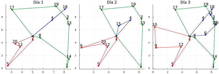
Total cost (z) = 152.62, T.CPU = 214.44 s
Lower_LB = 39.0%, Lower_BKS = −4.1%
Obtained routes with CPLEX Branch-and-Cut
Mathematics 13 01553 i002
Total cost (z) = 159.07, T.CPU = 3600.00 s
Lower_LB = 44.8%, Lower_BKS = 0.0%
Graphic of the solutions: Instance 8
Obtained routes of variant TSRIs—P and nMej = 50
Mathematics 13 01553 i003
Total cost (z) = 93.52, T.CPU = 208.41 s (each route is determined by a color)
Lower_LB = 32.8%, Lower_BKS = −5.5 p%
Obtained routes with CPLEX Branch-and-Cut
Mathematics 13 01553 i004
Total cost (z) = 98.93, T.CPU = 3600.00 s (each route is determined by a color)
Lower_LB = 40.5%, Lower_BKS = 0.0%
Graphic of the solutions: Instance 9
Obtained routes of variant TSRIs—P and  n M e j = 50
Mathematics 13 01553 i005
Total cost (z) = 165.07, T.CPU = 182.30 s (each route is determined by a color)
Lower_LB = 22.1%, Lower_BKS = − 0.2%
Obtained routes with CPLEX Branch-and-Cut
Mathematics 13 01553 i006
Total cost (z) = 165.47, T.CPU = 3600.00 s (each route is determined by a color)
Lower_LB = 22.4%, Lower_BKS = 0.0%

References

  1. Feillet, D.; Garaix, T.; Lehuédé, F.; Péton, O.; Quadri, D. A new consistent vehicle routing problem for the transportation of people with disabilities. Networks 2014, 63, 211–224. [Google Scholar] [CrossRef]
  2. Groër, C.; Golden, B.; Wasil, E. The consistent vehicle routing problem. Manuf. Serv. Oper. Manag. 2009, 11, 630–643. [Google Scholar] [CrossRef]
  3. Barros, L.; Linfati, R.; Escobar, J.W. An exact approach for the consistent vehicle routing problem (ConVRP). Adv. Prod. Eng. Manag. 2020, 15, 255–266. [Google Scholar] [CrossRef]
  4. Escobar, J.W.; Linfati, R.; Toth, P. A two-phase hybrid heuristic algorithm for the capacitated location-routing problem. Comput. Oper. Res. 2013, 40, 70–79. [Google Scholar] [CrossRef]
  5. Escobar, J.W.; Linfati, R.; Baldoquin, M.G.; Toth, P. A granular variable tabu neighborhood search for the capacitated location-routing problem. Transp. Res. Part B Methodol. 2014, 67, 344–356. [Google Scholar] [CrossRef]
  6. Tarantilis, C.D.; Stavropoulou, F.; Repoussis, P.P. A template-basedtabu search algorithm for the consistentvehicle routing problem. Expert Syst. Appl. 2012, 39, 4233–4239. [Google Scholar] [CrossRef]
  7. Kovacs, A.A.; Golden, B.L.; Hartl, R.F.; Parragh, S.N. The generalized consistent vehicle routing problem. Transp. Sci. 2015, 49, 796–816. [Google Scholar] [CrossRef]
  8. Xu, Z.; Cai, Y. Variable neighborhood search for consistent vehicle routing problem. Expert Syst. Appl. 2018, 113, 66–76. [Google Scholar] [CrossRef]
  9. Goeke, D.; Roberti, R.; Schneider, M. Exact and heuristic solution of the consistent vehicle-routing problem. Transp. Sci. 2019, 53, 1023–1042. [Google Scholar] [CrossRef]
  10. Rodríguez-Martín, I.; Salazar-González, J.J.; Yaman, H. The periodic vehicle routing problem with driver consistency. Eur. J. Oper. Res. 2019, 273, 575–584. [Google Scholar] [CrossRef]
  11. Stavropoulou, F.; Repoussis, P.P.; Tarantilis, C.D. The vehicle routing problem with profits and consistency constraints. Eur. J. Oper. Res. 2019, 274, 340–356. [Google Scholar] [CrossRef]
  12. Lespay, H.; Suchan, K. A case study of consistent vehicle routing problem with time windows. Int. Trans. Oper. Res. 2021, 28, 1135–1163. [Google Scholar] [CrossRef]
  13. Campelo, P.; Neves-Moreira, F.; Amorim, P.; Almada-Lobo, B. Consistent vehicle routing problem with service level agreements: A case study in the pharmaceutical distribution sector. Eur. J. Oper. Res. 2019, 273, 131–145. [Google Scholar] [CrossRef]
  14. Kulachenko, I.N.; Kononova, P.A. A Hybrid Local Search Algorithm for the Consistent Periodic Vehicle Routing Problem. J. Appl. Ind. Math. 2020, 14, 340–352. [Google Scholar] [CrossRef]
  15. Mancini, S.; Gansterer, M.; Hartl, R.F. The collaborative consistent vehicle routing problem with workload balance. Eur. J. Oper. Res. 2021, 293, 955–965. [Google Scholar] [CrossRef]
  16. Yao, Y.; Van Woensel, T.; Veelenturf, L.P.; Mo, P. The consistent vehicle routing problem considering path consistency in a road network. Transp. Res. Part B Methodol. 2021, 153, 21–44. [Google Scholar] [CrossRef]
  17. Yang, M.; Ni, Y.; Song, Q. Optimizing driver consistency in the vehicle routing problem under uncertain environment. Transp. Res. Part E Logist. Transp. Rev. 2022, 164, 102785. [Google Scholar] [CrossRef]
  18. Nolz, P.C.; Absi, N.; Feillet, D.; Seragiotto, C. The consistent electric-Vehicle routing problem with backhauls and charging management. Eur. J. Oper. Res. 2022, 302, 700–716. [Google Scholar] [CrossRef]
  19. Stavropoulou, F. The Consistent Vehicle Routing Problem with heterogeneous fleet. Comput. Oper. Res. 2022, 140, 105644. [Google Scholar] [CrossRef]
  20. Messaoudi, B.; Oulamara, A.; Salhi, S. A decomposition approach for the periodic consistent vehicle routeing problem with an application in the cleaning sector. Int. J. Prod. Res. 2023, 61, 7727–7748. [Google Scholar] [CrossRef]
  21. Kulachenko, I. Decomposition strategies for solving a large-scale consistent vehicle routing problem. In Proceedings of the 2023 19th International Asian School-Seminar on Optimization Problems of Complex Systems (OPCS), Novosibirsk, Russia, 14–22 August 2023; IEEE: Piscataway, NJ, USA, 2023; pp. 48–52. [Google Scholar]
  22. Ackva, C.; Ulmer, M.W. Consistent routing for local same-day delivery via microo-hubs. OR Spectr. 2024, 46, 375–409. [Google Scholar] [CrossRef]
  23. Yu, X.P.; Hu, Y.S.; Wu, P. The consistent vehicle routing problem considering driver equity and flexible route consistency. Comput. Ind. Eng. 2024, 187, 109803. [Google Scholar] [CrossRef]
  24. Alvarez, A.; Cordeau, J.F.; Jans, R. The consistent vehicle routing problem with stochastic customers and demands. Transp. Res. Part B Methodol. 2024, 186, 102968. [Google Scholar] [CrossRef]
  25. Wu, S.; Jin, C.; Bo, H. Exact solution of workload consistent vehicle routing problem with priority distribution and demand uncertainty. Comput. Ind. Eng. 2025, 202, 110940. [Google Scholar] [CrossRef]
  26. Glover, F. Tabu search—Part I. ORSA J. Comput. 1989, 1, 190–206. [Google Scholar] [CrossRef]
  27. Clarke, G.; Wright, J.W. Scheduling of vehicles from a central depot to a Number of delivery points. Oper. Res. 1964, 12, 568–581. [Google Scholar] [CrossRef]
  28. Avdoshin, S.; Beresneva, E. Constructive heuristics for Capacitated Vehicle Routing Problem: A comparative study. Proc. Inst. System. Program. RAS 2019, 31, 145–156. [Google Scholar] [CrossRef]
  29. Kouider, T.O.; Cherif-Khettaf, W.R.; Oulamara, A. Constructive Heuristics for Periodic Electric Vehicle Routing Problem. In Proceedings of the 7th International Conference on Operations Research and Enterprise Systems (ICORES 2018), Funchal, Portugal, 24–26 January 2018; pp. 264–271. [Google Scholar]
  30. Bolanos, R.; Escobar, J.; Echeverri, M. A metaheuristic algorithm for the multi-depot vehicle routing problem with heterogeneous fleet. Int. J. Ind. Eng. Comput. 2018, 9, 461–478. [Google Scholar] [CrossRef]
  31. Bolaños, R.; Echeverry, M.; Escobar, J. A multiobjective non-dominated sorting genetic algorithm (NSGA-II) for the Multiple Traveling Salesman Problem. Decis. Sci. Lett. 2015, 4, 559–568. [Google Scholar] [CrossRef]
  32. Camilo-Velandia, R.; Alvarez-Martinez, D.; Escobar, J.W. A metaheuristic algorithm based on Ant Colony Based approach for the assigning tasks problem to a workforce with different skills. Decis. Sci. Lett. 2024, 13, 729–740. [Google Scholar] [CrossRef]
  33. Escobar-Falcón, L.; Alvarez-Martinez, D.; Wilmer-Escobar, J.; Granada-Echeverri, M. A specialized genetic algorithm for the fuel consumption heterogeneous fleet vehicle routing problem with bidimensional packing constraints. Int. J. Ind. Eng. Comput. 2021, 12, 191–204. [Google Scholar] [CrossRef]
  34. Londoño, A.A.; Gonzalez, W.G.; Giraldo, O.D.M.; Willmer, J. A new matheheuristic approach based on Chu-Beasley genetic approach for the multii-depot electric vehicle routing problem. Int. J. Ind. Eng. Comput. 2023, 14, 555–570. [Google Scholar]
  35. Wang, H.; Yu, X.; Lu, Y. A reinforcement learning-based ranking teaching-learning-based optimization algorithm for parameters estimation of photovoltaic models. Swarm Evol. Comput. 2025, 93, 101844. [Google Scholar] [CrossRef]
Figure 1. Diagram of the process of the algorithm TSRI. Source: owner.
Mathematics 13 01553 g001
Figure 2. Insertion heuristic: initialize the routes. Source: owner. (nodes with color highlights the customers for which the insertion procedure is applied).
Mathematics 13 01553 g002
Figure 3. Insertion operator DC. Source: owner. Nodes are described by circles and arrows indicate the direction of the routes.
Mathematics 13 01553 g003
Figure 4. Operators: relocation, 2-opt intraroute, and inter-route exchange. Source: owner. Nodes are described by circles and arrows indicate the direction of the routes.
Mathematics 13 01553 g004
Figure 5. Multiroute operator 2-opt. Source: owner. Nodes are described by circles and arrows indicate the direction of the routes.
Mathematics 13 01553 g005
Figure 6. Feasible solutions and average lower-bound BKS. Source: owner.
Mathematics 13 01553 g006
Figure 7. Proportion of feasible solutions vs. the required consistency of schedules. Source: owner.
Mathematics 13 01553 g007
Figure 8. Performance of the different variants of the proposed approach. Source: owner.
Mathematics 13 01553 g008
Figure 9. Average computing time. Source: owner.
Mathematics 13 01553 g009
Figure 10. Statistics of the solutions vs. stage of the TSRI algorithm. Source: owner.
Mathematics 13 01553 g010
Figure 11. Average LB_BKS for the final solutions. Source: owner.
Mathematics 13 01553 g011
Table 1. Statistics of the final solutions.
ScenarioPopulation ParametersParameters of the Subset of Feasible Solutions
Variant
(Heuristic)
n M e j % Feasible Solutions %   Feasible   Sol :   z B K S Average Lower-Bound BKSDeviation Lower-Bound BKSAverage Lower BoundAverage CPU Time [s]
TSRI—A097.0%15.2%10.0%10.3%23.0%12.94
TSRI—A1097.0%51.5%3.3%6.5%15.3%26.02
TSRI—A5097.0%60.6%2.0%4.1%13.9%119.20
TSRI—P0100.0%3.0%10.5%10.5%23.4%9.38
TSRI—P10100.0%39.4%4.3%8.3%16.2%20.18
TSRI—P50100.0%60.6%2.1%5.2%13.7%101.63
TSRI—S0100.0%3.0%20.7%14.6%34.1%10.55
TSRI—S10100.0%39.4%4.7%6.3%16.6%19.40
TSRI—S50100.0%51.5%2.9%5.1%14.3%105.96
Source: owner.
Table 2. New Best-Known Solutions (BKS).
n I m p = 50
IdInst.CPLEX Branch-and-CutTSRI—ATSRI—PTSRI—S
LBz (BKS)T.CPU [s]zT.CPU [s]zT.CPU [s]zT.CPU [s]
620UC1109.84159.073600.00156.50211.14152.62214.44154.94208.57
820CC170.4398.933600.00100.39216.0893.52208.4193.52182.41
920CE1135.23165.473600.00165.50225.36165.07182.30168.62185.05
Source: Owner.
Disclaimer/Publisher’s Note: The statements, opinions and data contained in all publications are solely those of the individual author(s) and contributor(s) and not of MDPI and/or the editor(s). MDPI and/or the editor(s) disclaim responsibility for any injury to people or property resulting from any ideas, methods, instructions or products referred to in the content.

