Article

Forecasting Influenza Trends Using Decomposition Technique and LightGBM Optimized by Grey Wolf Optimizer Algorithm

1
School of Civil Engineering and Architecture, Henan University of Technology, Zhengzhou 450001, China
2
School of Civil Engineering and Environment, Zhengzhou University of Aeronautics, Zhengzhou 450046, China
3
School of Electronics and Information, Zhengzhou University of Aeronautics, Zhengzhou 450046, China
*
Author to whom correspondence should be addressed.
Mathematics 2025, 13(1), 24; https://doi.org/10.3390/math13010024
Submission received: 29 November 2024 / Revised: 20 December 2024 / Accepted: 24 December 2024 / Published: 25 December 2024

Abstract

:
Influenza is an acute respiratory infectious disease marked by its high contagiousness and rapid spread, caused by influenza viruses. Accurate influenza prediction is a critical issue in public health and serves as an essential tool for epidemiological studies. This paper seeks to improve the prediction accuracy of influenza-like illness (ILI) proportions by proposing a novel predictive model that integrates a data decomposition technique with the Grey Wolf Optimizer (GWO) algorithm, aiming to overcome the limitations of current prediction methods. Firstly, the most suitable indicators were selected using Spearman correlation coefficient. Secondly, a GWO-LightGBM model was established to obtain the residuals between the predicted and actual values. The residual sequence from the GWO-LightGBM model was then decomposed and corrected using the Complete Ensemble Empirical Mode Decomposition with Adaptive Noise (CEEMDAN) method, which led to the development of the GWO-LightGBM-CEEMDAN model. The incorporation of the Baidu Index was shown to enhance the precision of the proposed model’s predictions. The proposed model outperforms comparison models in terms of evaluation metrics such as RMSE and MAPE. Additionally, our study found that the revised Baidu Index indicators show a notable association with ILI trends.

1. Introduction

Influenza is an acute respiratory infection caused by influenza viruses [1]. It strikes rapidly, characterized by symptoms like high fever, headache, fatigue, conjunctivitis, and generalized muscle aches and pains. The disease is mainly spread through contact and airborne droplets, and is seasonally prevalent every year [2]. Compared to the common cold, influenza viruses are highly pathogenic, mutate easily, and have a greater tendency to spark outbreaks and epidemics. They also pose a higher risk of complications such as pneumonia, myocarditis, neurological damage, and even death. China, with its diverse geography and climate, experiences influenza epidemics that vary regionally. Studies have shown that influenza outbreaks are most common in winter and spring in Northern China, while in Southern China, they can occur throughout the year, peaking during summer and winter months [3].
In accordance with the World Health Organization, there are approximately 1 billion cases of seasonal influenza globally each year, including 3 to 5 million severe cases, resulting in 290,000 to 650,000 respiratory deaths annually [4]. Influenza surveillance is a crucial measure for the prevention and control of influenza, which can provide valuable epidemiological information to relevant departments and the public, and it holds immense practical significance in guiding and fostering the advancement of public health. Influenza-like illness proportion (ILI%) is an important indicator of influenza surveillance data [5]; when a certain threshold is reached, the relevant departments need to carry out influenza preventive and control measures to reduce the risk of influenza transmission. However, the inherent delay in ILI data released by the National Influenza Center of China, typically one to two weeks, necessitates the development of accurate predictive models to anticipate influenza activity and inform proactive measures [6]. By providing timely warnings, monitoring disease progression, and implementing countermeasures promptly, we can effectively mitigate the potential health risks associated with such outbreaks.

1.1. Literature Review

1.1.1. Prediction Models

The development of models serves as a valuable tool for enhancing the understanding of seasonal influenza patterns and providing practical guidance for public health departments [7]. Due to advancements in artificial intelligence, numerous models were successfully implemented to predict the proportion of influenza-like illnesses. Prediction methods are primarily categorized into three types: statistical models, machine learning models, and hybrid models. Among them, statistical models mainly encompass time series models and regression analysis models. Time series models, such as ARMA [8], ARIMA [9,10], and SARIMA [11], are widely used in influenza forecasting. For example, Qian et al. [12] utilized a seasonal autoregressive integrated moving average (SARIMA) model for forecasting the trend of the percentage of influenza-like illnesses in Shanghai. Their results demonstrated that the model was effective for medium term forecasting of ILI% in the city. This finding offers a valuable early warning system for influenza pandemics and outbreaks in Shanghai. In terms of regression modelling, Qin et al. [13] used the Joinpoint regression model to conduct a detailed analysis of the influenza incidence trends in Qinghai Province, China, and performed segmented analysis to study the long-term trends of influenza. Chen et al. [14] investigated the utility of the Least Absolute Shrinkage and Selection Operator (LASSO) model for real-time prediction of endemic infectious diseases through cross-country comparisons and explored differences in model prediction accuracy under various climatic conditions.
However, it is worth noting that time series and regression models are based on certain assumptions and have limited adaptability, which may lead to suboptimal performance when dealing with complex or non-linear data patterns. Consequently, some researchers have started employing machine learning models for influenza prediction, achieving promising results. For example, Signorini et al. [15] established a real-time tracking and prediction model for the percentage of flu cases in the United States using the support vector regression (SVR) model based on Twitter data. Tsan et al. [16] conducted empirical research using datasets with two different time spans, comparing the ARIMA and LSTM models. Finally, they proved that the LSTM model performed three to seven times better than the ARIMA model. Manohar and Das [17] developed a method for predicting the monkeypox outbreak in the USA, Germany, UK, France, and Canada by comparing different artificial neural network models (including ANN, LSTM, and GRU), with the ANN model demonstrating the best performance in prediction.
In dealing with the prediction problem however single machine learning models often exhibit disadvantages such as the tendency to fall into local minima or the phenomenon of overfitting [18]. After the predictions made by single machine learning models, a series of non-purely random and non-linear residual sequences still exist. Therefore, in terms of influenza prediction, high accuracy prediction of target values can be achieved by integrating decomposition techniques, optimization algorithms, and machine learning models into a new hybrid model, which combines the advantages of the three algorithms and improves the robustness and stability of the model. This approach has already proven successful in various fields, such as finance and energy. For instance, Liang et al. [19] used improved Complete Ensemble Empirical Mode Decomposition With Adaptive Noise method and a combined LSTM-CNN-CBAM model to realize high-precision prediction of gold futures and spot prices. In order to predict the international crude oil price, Liao [20] proposed a hybrid model combining VMD and LSTM-ELMAN. The findings from empirical research indicate that the proposed model VMD-LSTM-ELMAN has strong validity and reliability compared to others. However, models with decomposition technique are rarely applied in influenza prediction. Therefore, this study aims to utilize a decomposition model to predict influenza in Southern China.

1.1.2. Influence Factors

Recent research indicates that, in the context of the big data era, online public opinion has emerged as the primary platform for information dissemination, with internet users relying heavily on search engines as a primary source of knowledge acquisition. Therefore, big data such as online public opinion can help us in predicting influenza trends. Since 2008, web search data have gradually garnered significant attention from scholars both domestically and internationally, emerging as a thriving research topic. For instance, Ginsberg et al. [21] utilized the output data from Google health search engine software to predict influenza-like cases in the United States and verified the accuracy of the model. In China, Baidu search engine has become the primary method for searching information, and the Baidu Search Index has emerged as a unique data type. Yuan et al. [22] pioneered the use of filtered Baidu Index data for predictive modelling to forecast monthly flu cases in China, achieving commendable results.
The core objective of this study is to propose a method for predicting influenza trends based on the Baidu Index. This method employs a currently mainstream machine learning model, LightGBM, as the benchmark model, which incorporates the Grey Wolf Optimizer (GWO) to enhance predictive capabilities and introduces the Complete Ensemble Empirical Mode Decomposition with Adaptive Noise (CEEMDAN) technique to address residuals in the prediction data. Through the integration of these techniques, this study has developed a novel prediction model, namely GWO-LightGBM-CEEMDAN, which aims to provide a scientific basis for public health monitoring departments in the prediction of infectious diseases.

1.2. Gaps and Contributions

After conducting an exhaustive review of the existing literature on influenza prediction models, this study has identified several research gaps.
  • Existing research in influenza forecasting often relies solely on historical time series data or a single Baidu Index, whereas this study innovatively integrates both the Baidu Index and historical autocorrelation data to construct a more comprehensive and accurate influenza prediction model. By merging these datasets, we can capture influenza trends more holistically, enhancing the precision and reliability of our forecasts and addressing the deficiencies in current research.
  • In existing influenza prediction research using the Baidu Index, a significant gap is the neglect of feature selection. Spearman correlation analysis is essential for addressing this, as it allows for the careful screening and selection of input features, reducing dimensionality while preserving critical information, potentially enhancing model predictive accuracy.
  • Existing research indicates that the application of decomposition techniques in the field of influenza prediction is not widespread. Despite the advancements achieved by machine learning models in predicting influenza trends, they still face challenges in avoiding overfitting and escaping local minima. Consequently, the incorporation of decomposition algorithms is expected to enhance the model’s capability to capture influenza trends by providing a multiscale analysis, while simultaneously reducing the risk of overfitting.
The contributions and novelties of this study are summarized as follows:
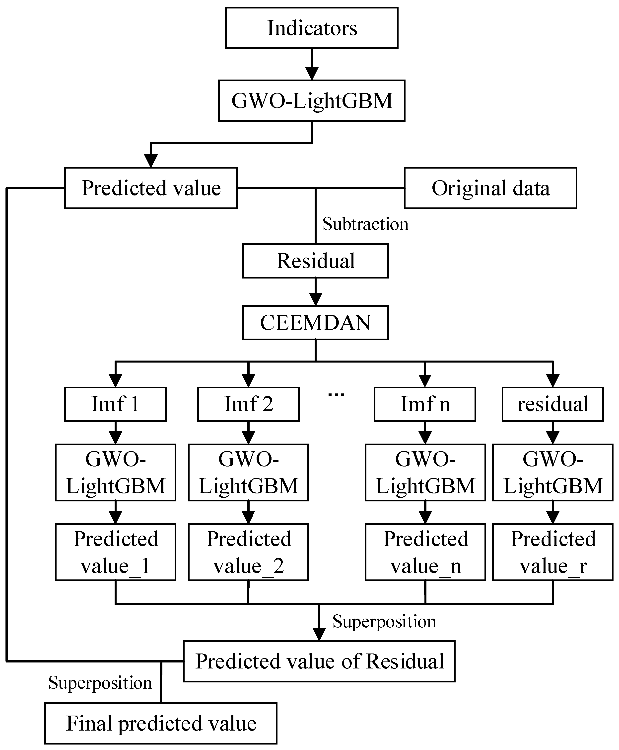
  • In this study, we propose an innovative influenza trend prediction model, GWO-LightGBM-CEEMDAN, which integrates optimization algorithms with decomposition techniques. Unlike the conventional process of most existing models that proceed with decomposition before prediction, our model adopts a unique strategy of predicting first and then decomposing. Specifically, following the initial prediction, we apply the CEEMDAN algorithm to process the residual series, addressing potential instability issues. Ultimately, experimental results confirm the practicality and superiority of this approach.
  • The Baidu Index is incorporated as an external influencing factor for prediction, realizing the application of big data in influenza prediction. This study adds Baidu Index as influencing factors on the basis of the original data and realizes the prediction with the help of internet search engine. In addition, compared to traditional big data, this study has updated the selection of the Baidu Index by adding new indices such as lymphocyte and nebulizer. The empirical analysis proves that the addition of the Baidu Index can improve the predictive ability of the model.
  • Previous studies using the Baidu Index for influenza prediction often neglected the feature selection of input data; therefore, to compensate for this deficiency, this study uses Spearman correlation analysis to filter the input features in order to reduce the dimensionality of the data and retain the most important data information, which in turn improves the prediction performance of the model.
The rest of this paper is structured as follows: Section 2 presents the experimental data and main methods covered in the research. Section 3 presents the experimental process and results. Section 4 is the discussion of the experimental results. Section 5 summarizes the main conclusions of this study and gives relevant policy recommendations and suggestions for future work.

2. Materials and Methods

2.1. Data Collection and Preprocessing

2.1.1. Data Source

An influenza-like illness is defined as a case with fever (a temperature of 38 °C or higher) accompanied by either cough or sore throat. The percentage of influenza-like illnesses in the total number of outpatient and emergency department cases is referred to as ILI%, which can reflect the development trend of influenza, and when it reaches a certain threshold, the public health authorities need to take relevant work in a timely manner in order to avoid an influenza pandemic. Therefore, in this study, we chose ILI% in Southern China as the research object, which was obtained from the Influenza Weekly Report on the website of the Chinese National Influenza Center (https://ivdc.chinacdc.cn/cnic/zyzx/, accessed on 25 February 2024).
The dataset selected for this study covers weekly data from 1 January 2019, to 31 December 2023, with a total of 261 samples. In this experiment, the first 80% of the dataset (from week 1 of 2019 to week 52 of 2022) is used as the training set, while the remaining 20% (from week 1 of 2023 to week 52 of 2023) serves as the test set. Figure 1 shows a line graph of the temporal distribution of ILI% in Southern China from week 1 of 2019 to week 52 of 2023. As can be seen from Figure 1, the ILI% values in the southern provinces were centrally distributed between 2% and 10%, with peak values occurring in the winter of 2022. Table 1 demonstrates the descriptive statistics of the experimental data.
As network information technology continues to advance, real-time monitoring of internet data has become feasible, enabling the Baidu Index to effectively capture interest and attention of users towards specific keywords. Foreign studies focus on the use of Google search engine data [21] and Twitter data, whereas in China, research primarily relies on the Baidu Index as a key data source [6]. During influenza epidemics, people turn to search engines such as Baidu to search for relevant terms and seek helpful information. Therefore, the Baidu Index is able to reflect the prevalence of a disease in its epidemic stage and can be used as an early warning system for early epidemics [23,24,25]. In this study, the external influencing factors were summarized into three categories with 37 related terms compiled: influenza prevention, symptoms and treatment by reviewing related literature [26], and collecting information. The Baidu Index data, collected on the official Baidu Index page interface (https://index.baidu.com/, accessed on 28 February 2024) through web crawler technology for the daily data from 1 January 2019, to 31 December 2023, is publicly accessible. To ensure data frequency consistency, the EViews 13 software was utilized to convert the daily data into a weekly format. Specific indicators are shown in Table 2.

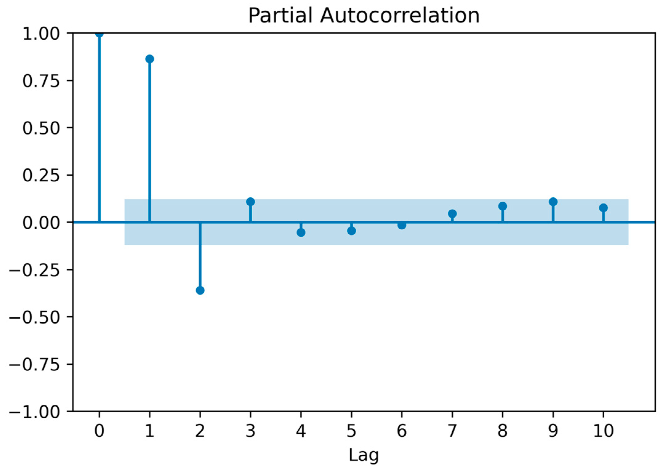
2.1.2. Data Analysis

Considering the inherent time-dependent nature of influenza incidence [7], this study tries to incorporate historical lag input features as part of the input variables for the prediction model. To evaluate the autocorrelation among historical data, the Partial Autocorrelation Function (PACF) approach was employed to select historical ILI% data as input variables [27]. Firstly, it is essential to perform an Augmented Dickey–Fuller (ADF) test [28] on the time series data; the results are presented in Table 3. Clearly, it is apparent that the ADF statistic value is –4.17 at 0th order difference, which is smaller than the critical values of 1%, 5%, and 10% level, and the p-value is 0.001, which is smaller than 0.05, presenting significance at the level of rejecting the original hypothesis. This outcome suggests that the original time series is stationary, allowing for direct analysis of its partial autocorrelation. Figure 2 demonstrates the results of the PACF for the ILI% data in Southern China. The results show that the ILI% data have second-order autocorrelation. Consequently, by letting Yi represent the output feature, the historical input variables for the dataset can include Yi-1 and Yi-2.
However, it is not necessarily the case that the more input features there are, the higher the accuracy of the model. Thirty-seven Baidu indices selected as external input features in this experiment may reduce prediction accuracy due to redundancy [29], so this study utilizes Spearman correlation to calculate and analyze the correlation between the external input features and ILI%, and then filter out the Baidu Index keywords that are most capable of influencing ILI%. This study uses the IBM SPSS Statistic 27 statistical tool for Spearman correlation analysis [30,31], and the results are shown in Table 4. It can be found that there are 32 keywords with p-value < 0.05, showing significant correlation in the indicator system of influenza-like case percentage established in this study. The p-values of X10, X17, X20, X24, and X26 exceed 0.05, suggesting no significant correlation between these five keywords and ILI%. Additionally, X21 was excluded from the model due to its p-value exceeding 0.01, aimed at enhancing prediction accuracy. Among the symptoms, considering the fact that routine blood indicators are useful for clinical disease diagnosis, elevated lymphocytes are generally indicative of viral infections [32]. Therefore, we ultimately added the key search term lymphocytes. In terms of treatment, the words selected for this study are not only specific drugs, but also added the medical device nebulizer, which can be used at home to do nebulization for symptoms such as coughing and sore throat, which was significantly correlated with the study population after Spearman correlation analysis. Therefore, in this study, the final input variables of the ILI% forecasting model are as follows: {X1, X2, X3, X4, X5, X6, X7, X8, X9, X11, X12, X13, X14, X15, X16, X18, X19, X22, X23, X25, X27, X28, X29, X30, X31, X32, X33, X34, X35, X36, X37, Yi-1, Yi-2}.

2.1.3. Data Processing

Normalizing the collected data, which exhibits varying orders of magnitude and units, is crucial to eliminate order of magnitude errors, enhance comparability, and ensure precise and reliable analysis. This serves to simplify the process of comparison and analysis, and to enhance the accuracy and efficacy of machine learning algorithms. The mathematical expression for normalization is as follows:
x * = x x m i n x m a x x m i n
where x* is the normalized value, x is the original data, xmin is the minimum value in the dataset, and xmax is the maximum value in the dataset. The normalized data falls within the range of [0,1], ensuring comparability and consistency across datasets.

2.2. Models

2.2.1. GWO Algorithm

The Grey Wolf Optimizer (GWO) algorithm was developed by Mirjalili et al. [33] in 2014 as a meta-heuristic algorithm based on group intelligence, which is inspired by the social structure of grey wolf populations. In the social hierarchy of grey wolves, there are four different ranks of grey wolves, including α-wolves, β-wolves, δ-wolves, and ω-wolves, whose social status decreases from left to right, and the superior grey wolves have absolute dominance over the inferior grey wolves.
The four levels of pack wolves represent the four solutions searched by the GWO optimization process, with α-wolf representing the optimal solution, β-wolf and δ-wolf as the two suboptimal solutions, and ω-wolf as the candidate solution. The top three most outstanding wolves are designated as α, β, and δ wolves, who lead the other wolves in their pursuit towards achieving the objective. Meanwhile, the remaining wolves are categorized as ω wolves, who adjust their position in relation to α, β, or δ wolves. This includes steps such as the social hierarchy of grey wolves, encirclement, hunting, and attacking prey, as described below.
1.
Social class of grey wolf
Calculate and assess the fitness of each member of the population. The three grey wolves with the highest fitness were labelled α, β, and δ, respectively.
2.
Surrounding
During the hunt, grey wolves employ specific position update formulas to effectively encircle their prey.
D = C · X p t X t
t + 1 = X p t A · D
where D represents the distance between the grey wolf and its prey; A and C are coefficient vectors; t is the number of iterations; and X p t and X t are the position vectors of the prey and the grey wolf, respectively, after t iterations. A and C are calculated as follows:
A = 2 a · r 1 a
C = 2 · r 2
a = 2 2 t T m a x
where a denotes the convergence factor and it decreases linearly from 2 to 0 as the iterations progress; r 1 and r 2 are random vectors in the range [0,1]; and T m a x is the maximum number of iterations.
3.
Hunting
Once the grey wolf identifies the location of its prey, it leads the pack to encircle the target under the guidance of α, β, and δ wolves. The mathematical model describing an individual grey wolf’s tracking of the prey’s location is outlined as follows:
D α = C 1 · X α X
D β = C 2 · X β X
D δ = C 3 · X δ X
where D α , D β , and D δ denote the distances between α, β, and δ and other individuals, respectively; X α , X β , and X δ represent the current positions of α, β, and δ, respectively; C 1 , C 2 , and C 3 are random vectors; and X is the current position of the grey wolf.
X 1 = X α A 1 · D α
X 2 = X β A 2 · D β
X 3 = X δ A 3 · D δ
X t + 1 = X 1 + X 2 + X 3 3
X 1 , X 2 , and X 3 denote the positions affected by α-layer wolves, β-layer wolves, and δ-layer wolves, respectively, and Equation (13) is the position of an ω grey wolf individual that needs to be adjusted. X t + 1 denotes the updated position of the grey wolf after the tth iteration, which corresponds to the initial position of the grey wolf at the (t+1)th iteration. The algorithm keeps iterating until there is no significant change in the position of the grey wolf between two consecutive iterations, indicating that the grey wolf has successfully captured the prey, and the algorithm stops iterating.
4.
Attacking prey
In the process of constructing the model of attacking prey, the decrease in a value will lead to the fluctuation of a value. The grey wolf mainly relies on the information of α, β, and δ to find prey.
When addressing optimization problems using GWO, it is imperative to possess an objective function, as the primary goal of the algorithm is to identify the solution that optimizes the value of this function. In the context of our experiments, the objective function is the fitness function, which aims to calculate the mean absolute error (MAE). The optimal solution corresponds to the set of parameters that yield the minimum MAE. Furthermore, GWO can be applied to both minimization and maximization problems; however, the algorithm employed in this research is based on the minimization of the problem. The pseudocode of the GWO algorithm is detailed in Algorithm 1.
Algorithm 1. GWO algorithm pseudocode.
Inputs: Grey wolf population Xi; maximum number of iterations Imax
Output: The best agent position Xα
Process:
Initialize Xi, (i = 1, 2, …, n), a, A and C
Calculate the fitness of each Xi to choose the best three solutions Xα, Xβ and Xδ
While (t < Imax)
 for each Xi
  Update the position of the current search agent
 end for
 Update a, A and C
 Calculate the fitness of all search agents
 Update Xα, Xβ and Xδ
 t = t + 1
End while
Return Xα

2.2.2. LightGBM Model

Light Gradient Boosting Machine (LightGBM) [34] is a gradient boosting decision tree based on a gradient boosting decision tree [35] released by Microsoft in 2017 of an improved iterative boosting tree system, similar in principle to GBDT. The method constructs a fresh decision tree by employing the negative gradient of the loss function as an approximation of residuals relative to the existing decision tree. During each iteration, the original model remains intact while new functions are incorporated to progressively minimize the discrepancy between predicted and measured values.
Suppose a set of datasets M = x i , y i 1 N , where x = x 1 ,   x n are input features and y is the label. F(x) is the model function and L (y, F(x)) is the model loss function. The key aspect of gradient boosting is the adoption of the negative gradient of the loss function L, given the current value of the model function F(x), as an alternative approach to residuals. Let gij be the negative gradient of the jth iteration, then we can obtain the following:
g i j = L y i , F x i F x i F x = F j 1 x
Designating h(x) as the weak learner, we utilize it to match the negative gradient of the loss function, ultimately determining the most appropriate fit value as follows: g i = arg m i n g   L y i , F j 1 x i + g h j x i . At this point the model update equation is F j x = F j 1 x + g i h j x .
In the aforementioned manner, gradient boosting undergoes iterative updates, training individual weak learners sequentially. Upon completion of the iteration process, the weak learners are linearly combined to yield the strong learners.
LightGBM uses a histogram-based approach to approximate the selection of the best decision tree splits to reduce computational complexity. Meanwhile, a leaf-wise growth strategy is used to select the node with the largest gradient for splitting each time to quickly generate deeper trees. The parallelization technique enables LightGBM to take full advantage of multi-core processors and distributed computing environments to speed up training.

2.2.3. CEEMDAN Algorithm

Complete Ensemble Empirical Mode Decomposition with Adaptive Noise (CEEMDAN) is a novel data decomposition technique introduced by Torres et al. [36] in 2011, which aims to solve the problem of the noise introduced by the Ensemble Empirical Mode Decomposition (EEMD) algorithm corrupting the original signal, and it better solves the phenomenon of mode aliasing in empirical mode decomposition. The CEEMDAN algorithm adjusts the noise coefficients adaptively in each stage of the EMD decomposition of the signal thus introducing Gaussian noise with different signal-to-noise ratios into the signal to be decomposed, avoiding the problem of mode aliasing and eliminating the false information interference simultaneously. Noise in the signal to be decomposed can simultaneously help avoid the modal aliasing problem and eliminate false information interference. Since the decomposition of this method is complete, the original signal can be reconstructed accurately by summing the IMFs.
The principle of CEEMDAN algorithm is as follows:
Step1: The positive and negative Gaussian white noise of N pairs are added to the original signal x(t) to obtain N new signals. After adding Gaussian white noise for ith time, the new signal is as follows:
x 0 i ( t ) = x t + ε 0 ω i ( t )
where ε 0 is the noise standard deviation and ω i is the ith Gaussian white noise satisfying the standard normal distribution.
Srep2: Let E(*) be the sequence after EMD decomposition, and the ith component IMF1 can be obtained by decomposition of i times; the formula is as follows:
E x 0 i ( t ) = I M F 1 i t + r i t
where I M F 1 i t is the ith IMF1 component; and r i t is the ith residual component.
Step3: The N IMF1 components obtained by decomposition are summed and averaged to obtain the final IMF1(t) as follows:
I M F 1 ( t ) = 1 N i = 1 N I M F 1 i ( t )
Step4: The first residual term r1(t) is calculated according to the formula as follows:
r 1 t = x t I M F 1 ( t )
Step5: Add Gaussian white noise to r1(t) to obtain a new signal, and EMD decomposition is performed on the new signal. Let Eh(*) be the nth modal component after EMD decomposition, then the new signal after adding auxiliary noise for the ith time is as follows:
x 1 i ( t ) = r 1 t + ε 0 E 1 ω i ( t )
By decomposing the new signal for the ith time, the ith IMF2 component is obtained, and the decomposition result is as follows:
E x 1 i ( t ) = I M F 1 i t + r i t
Summing the N IMF2s obtained by decomposition and take the average value to obtain IMF2(t) as follows:
I M F 2 ( t ) = 1 N i = 1 N I M F 2 i ( t )
Calculating the second residual component, we can obtain r2(t) in the following equation:
r 2 ( t ) = r 1 t I M F 2 ( t )
Step6: Repeat the above steps until the obtained residual term can no longer proceed with EMD decomposition and the algorithm ends. Let the number of eigenmode components be K, then the original signal x(t) is decomposed as follows:
x t = k = 1 K I M F k t + r k ( t )
After decomposing the original series by using CEEMDAN, each eigenmode function component along with the trend term undergoes individual prediction by employing an appropriate prediction model. Subsequently, the outcomes obtained from each individual component are linearly merged to generate the ultimate residual prediction.

2.2.4. GWO-LightGBM-CEEMDAN Model

A GWO-LightGBM-CEEMDAN model is proposed in this study as a means of improving the prediction of the influenza-like illness consultation rate. It combines GWO, LightGBM, and CEEMDAN algorithms in order to create a more accurate prediction. Figure 3 presents a detailed overview of the model introduced in this study, outlined as follows:
Step 1: Make preliminary projections. The LightGBM model is established, and its parameters are optimized using the GWO algorithm. Subsequently, the model that was just optimized is utilized to obtain initial prediction of ILI%.
Step 2: Obtain the residual. Subtract the original data from the initial predicted value to obtain the residual sequence.
Step 3: Decompose the residual. The residual sequence of the GWO-LightGBM model was decomposed using the CEEMDAN technique, resulting in multiple intrinsic modal components and a trend component.
Step 4: Obtain the predicted value of the residual. Each of these components, including the residual, was then predicted separately using the GWO-LightGBM model. The predictions were summed up to obtain the predicted value of the residual.
Step 5: Obtain the final predicted value. The initial prediction obtained from the GWO-LightGBM model is summed with the predicted value of the residual to arrive at the final predicted value of the proposed model in this research.
It should be noted that the input data used to acquire the initial prediction values were 31 Baidu indices and ILI% historical data, while the input data used for the second prediction after residual decomposition was only historical lag data.

2.3. Evaluation Indicators

To visually assess the predictive capabilities of each model, this study employs multiple evaluation metrics, including root mean square error (RMSE), mean absolute error (MAE), mean absolute percentage error (MAPE), and R-squared (R2). RMSE is the square root of the average of the squared differences between the predicted and actual values, and is used to measure the magnitude of prediction error; MAE is the average of the absolute differences between the predicted and actual values, and is used to measure the average magnitude of the prediction error; MAPE is the average of the absolute differences between the predicted and actual values as a percentage of the actual values, and is used to measure the relative magnitude of the prediction error; and R² represents the proportion of the variance in the dependent variable that is explained by the independent variables in a regression model, and is used to measure the goodness of fit of the model [37,38,39,40]. Collectively, these metrics offer a comprehensive understanding of model performance. Specifically, a model is considered more accurate when MAE, RMSE, and MAPE values are low and the R2 value is high [41,42]. The mathematical formulas for each metric are outlined as follows:
R M S E = 1 n i = 1 n ( y ^ i y i ) 2
M A E = 1 n i = 1 n ( y ^ i y i )
M A P E = 100 % n i = 1 n y ^ i y i y i
R 2 = 1 i = 1 n y ^ i y i 2 i = 1 n y ¯ i y i 2
where n represents the number of samples, y i denotes the actual value of ILI%, y ^ i denotes the predicted value of ILI%, and y ¯ i denotes the mean value of ILI%.

3. Empirical Analysis and Results

In this study, the GWO-LightGBM algorithm was used to predict each modal component after decomposition separately, and the final prediction value of ILI% was obtained by accumulating the prediction values of each component with the residuals. The proposed model is validated using the percentage data of influenza-like illness cases in Southern China. For the purpose of demonstrating the superiority of the GWO-LightGBM-CEEMDAN model in predicting ILI%, five different models are also constructed in this paper to compare with the proposed model, which are XGBoost, LightGBM, WOA-LightGBM, GWO-LightGBM, and GWO-LightGBM-EEMD.

3.1. Experimental Environment and Parameter Settings

This research is in the virtual environment of Python 3.10 on Anaconda 2.4.0, using a Windows11 system laptop with an Intel Core i5-13500H CPU, Intel(R) Iris(R) Xe Graphics GPU, and 16G RAM.
In this study, multiple models were used as comparisons. For the single model, XGBoost and LightGBM are used for comparison and analysis; in the combined model, WOA and GWO are first used for comparison, followed by EEMD and CEEMDAN. The following explains the rationale behind certain parameter settings. The two single machine learning models chosen in this experiment are widely popular algorithms in recent years. As they are used as benchmark experiments in this study, their parameters are set to default values. The predictive performance of LightGBM is primarily affected by n_estimators, num_leaves, learning_rate, and max_depth [43,44], so we choose to optimize the four parameters. Figure 4 illustrates the fitness convergence curves of the WOA and GWO algorithms in solving this experimental problem. The results indicate that GWO achieved a rapid reduction in fitness within the first 13 iterations and stabilized approximately, whereas WOA begins to stabilize after 19 iterations. GWO ultimately attained a lower fitness value compared to WOA at the termination of iterations, indicating its superior performance in identifying the optimal solution for this study. For the sake of fairness, we set the same parameters for the two optimization algorithms. According to the previous study [45], the optimization algorithm parameters for this experiment are set to 30 iterations and a population size of 20.
Table 5 provides the parameter settings of each algorithm in this experiment, where WOA-LightGBM and GWO-LightGBM show the parameter values of both after their respective optimizations. Figure 5 shows the resulting images of the CEEMDAN decomposition from the experiment.

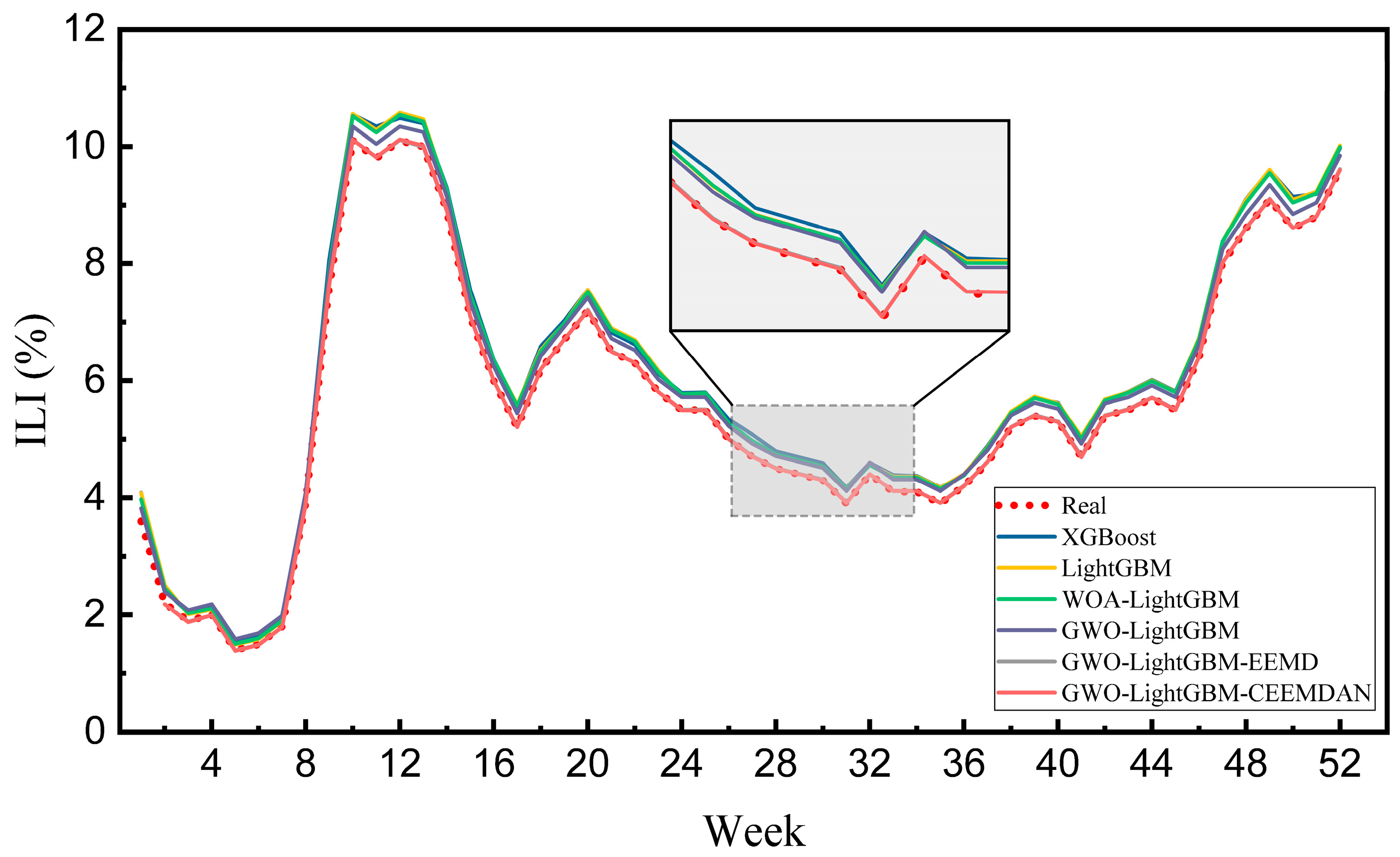
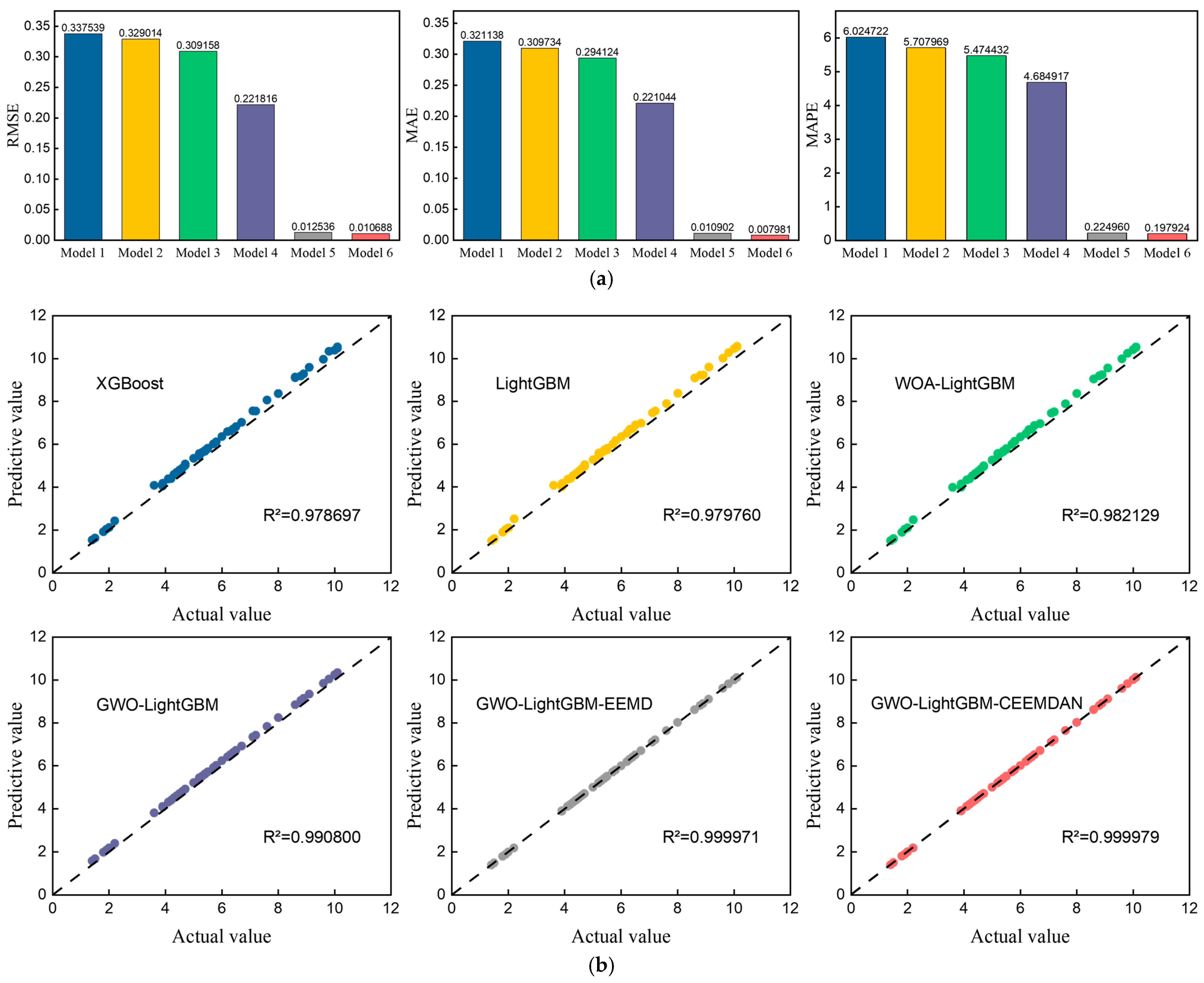
3.2. Experimental Results

Among the benchmark models chosen in this study, XGBoost, LightGBM, WOA-LightGBM, and GWO-LightGBM serve as prediction models that do not incorporate decomposition techniques, while GWO-LightGBM-EEMD and GWO-LightGBM-CEEMDAN are models that integrate distinct decomposition methods. The GWO-LightGBM-EEMD model first predicts the original ILI% data with GWO-LightGBM, the residuals are obtained by differencing the original data and the prediction results of this model, then this residual is decomposed to obtain multiple components using the EEMD method, and then the residuals are decomposed again with the GWO-LightGBM model for each IMF component of the residuals. Each IMF component of the residual is then predicted again using the GWO-LightGBM model and summed up to compute the predicted residual value; the predicted value of the residual is ultimately summed up with the values of the data predicted by the GWO-LightGBM to form the final prediction result. The GWO-LightGBM-CEEMDAN model operation steps are the same as above, except that the decomposition technique uses the CEEMDAN technique. The characteristics of all models are presented in Table 6.
The real value and predicted values of the six models are shown in Figure 6. The specific prediction results of each model are shown in Table 7 and Figure 7. The empirical results of the study demonstrate that, in contrast to other benchmark models, the GWO-LightGBM-CEEMDAN model demonstrates superior predictive performance for ILI% prediction in Southern China. After comparing the empirical results, we can draw some conclusions.
First, in the single prediction model results, the LightGBM model has better prediction performance than the XGBoost model. Although both models are based on the gradient boosting decision tree algorithm, the fact that LightGBM employs a histogram-based decision tree algorithm enables it to have better computational efficiency when dealing with large data, in contrast to XGBoost, which uses a pre-order-based decision tree algorithm, which makes it slower when dealing with large datasets. In addition, LightGBM uses a leaf-wise growth strategy that helps to find more accurate models, which improves the performance of the model to some extent.
Second, the prediction accuracies of MSE, MAE, and RMSPE are improved after adding the Whale Optimization Algorithm and Grey Wolf Optimization to the LightGBM model compared to the unoptimized model. The results suggest that optimization algorithms can help to identify the optimal parameter values for the base model thereby enhancing the predictive accuracy of the model. In addition, GWO is able to find better model parameters than WOA in this study.
Third, the models with the decomposition technique show a great improvement in accuracy in all the metrics. Compared to GWO-LightGBM, the predictive accuracy of GWO-LightGBM-EEMD is greatly improved, RMSE and MAE are improved by 94.35% and 95.07%, and R2 has improved by 0.93%, while the RMSE and MAE of the model with CEEMDAN technique are improved by 95.18% and 96.39%, respectively. This indicates that the residual term contains rich data information, decomposition techniques can simplify the intricacy of the data series, and the overall prediction performance of the model can be improved by decomposing the residuals.
In addition, by comparing Model 5 and Model 6, it can be found that the CEEMDAN technique is superior to EEMD in terms of decomposition methods. Compared to Model 5, the RMSE, MAE, and MAPE of Model 6 are improved by 14.74%, 26.79%, and 12.02%, respectively, and it can be concluded that CEEMDAN has a stronger ability.

3.3. Experiment II: Comparison of Model Proposed in This Paper with Different Input Indicators

In order to demonstrate the importance of the added external influences (Baidu Index), this study conducted another experiment (Experiment II) to illustrate the superiority of the proposed model. Therefore, we set up a new model, GWO-LightGBM-CEEMDAN’, in Experiment II, and the input data of this model is based on the data of the first experiment but without 31 Baidu indices. It should be pointed out that GWO-LightGBM-CEEMDAN’ did not delete Yi-1 and Yi-2 or change the values of each algorithm parameter. The detailed prediction results are shown in Table 8. It can be known that after deleting the Baidu Index, the evaluation indicators of the six models worsened. Therefore, it can be concluded that the addition of the Baidu Index has important and positive significance for predicting the ILI%.

4. Discussion

The monitoring and prediction of influenza are crucial tasks for public health departments. However, due to delays in the release of official data reports, public health departments cannot promptly assess the evolving trend of influenza, necessitating the prediction of ILI%. Most scholars primarily rely on time series models for prediction, overlooking the relevance of search-related terms on the internet. Relevant studies suggest that with the advent of information technology, individuals often seek medical information through search engines, such as symptoms, prevention, and treatment methods for the flu. As a result, changes in online search patterns can serve as indicators of the prevalence of infectious diseases. Given this, Baidu Index can serve as an influencing factor in predicting the trend of influenza, which is confirmed in this study.
Based on the experimental results presented above, we performed a comparative analysis of adjacent progressive hierarchical models, dividing them into four hierarchical groups. The improvement percentage of the models is shown in Table 9. The experimental findings clearly demonstrate that the proposed model outperforms all the comparative models. Furthermore, the incorporation of decomposition algorithms significantly improves the predictive performance of the model. Additionally, CEEMDAN exhibits superior decomposition effectiveness compared to EEMD, as evidenced by improvements between adjacent hierarchical levels. According to Spearman correlation analysis, it is evident that there is a strong correlation between most Baidu indices and ILI%. Furthermore, Table 9 demonstrated that incorporating the Baidu Index into the dataset can also improve the performance of the model.
Due to the large geographical and climatic differences between the south and the north, the peak of flu incidence in the two regions is different. Therefore, the model introduced in this research exhibits a robust predictive capability in determining the trend of influenza incidence in Southern China. Currently in the new crown post epidemic era, people’s health awareness is becoming stronger and their concern for diseases is increasing day by day. In addition, the epidemic has prompted the public health sector to accelerate its digital transformation, and the use of machine learning models to analyze historical epidemiological data as well as to learn from seasonal changes, network data, and other factors can be used to more quickly and accurately predict future trends in the spread of the disease. Public health departments can use the relevant models to predict future ILI% values in advance. When the ILI% rises to a certain threshold, the relevant departments will need to formulate preventive and control measures in a timely manner and send out early warning messages to the public, in the hope of reducing the spread of influenza. The current era is full of challenges and opportunities for the public health sector. Epidemiological surveillance departments need to continuously detect the spread of epidemics and utilize AI technology to improve the prevention and control system as well as prevention and control capabilities.

5. Conclusions

An influenza prediction model for Southern China is proposed in this study, which integrates external factors and historical data by using a data decomposition method and a feature engineering selection technique. To corroborate the efficacy of the introduced model, we conducted an empirical study on the ILI% data of Southern China from 2019 to 2023, and systematically and comprehensively validated the reasonableness and validity of the GWO-LightGBM-CEEMDAN model by means of five comparative models, four evaluative indicators, and two experiments. Therefore, we believe that the framework formulated in this paper provides a valuable model to predict influenza epidemic trends. The findings of this study can be briefly summarized as follows:
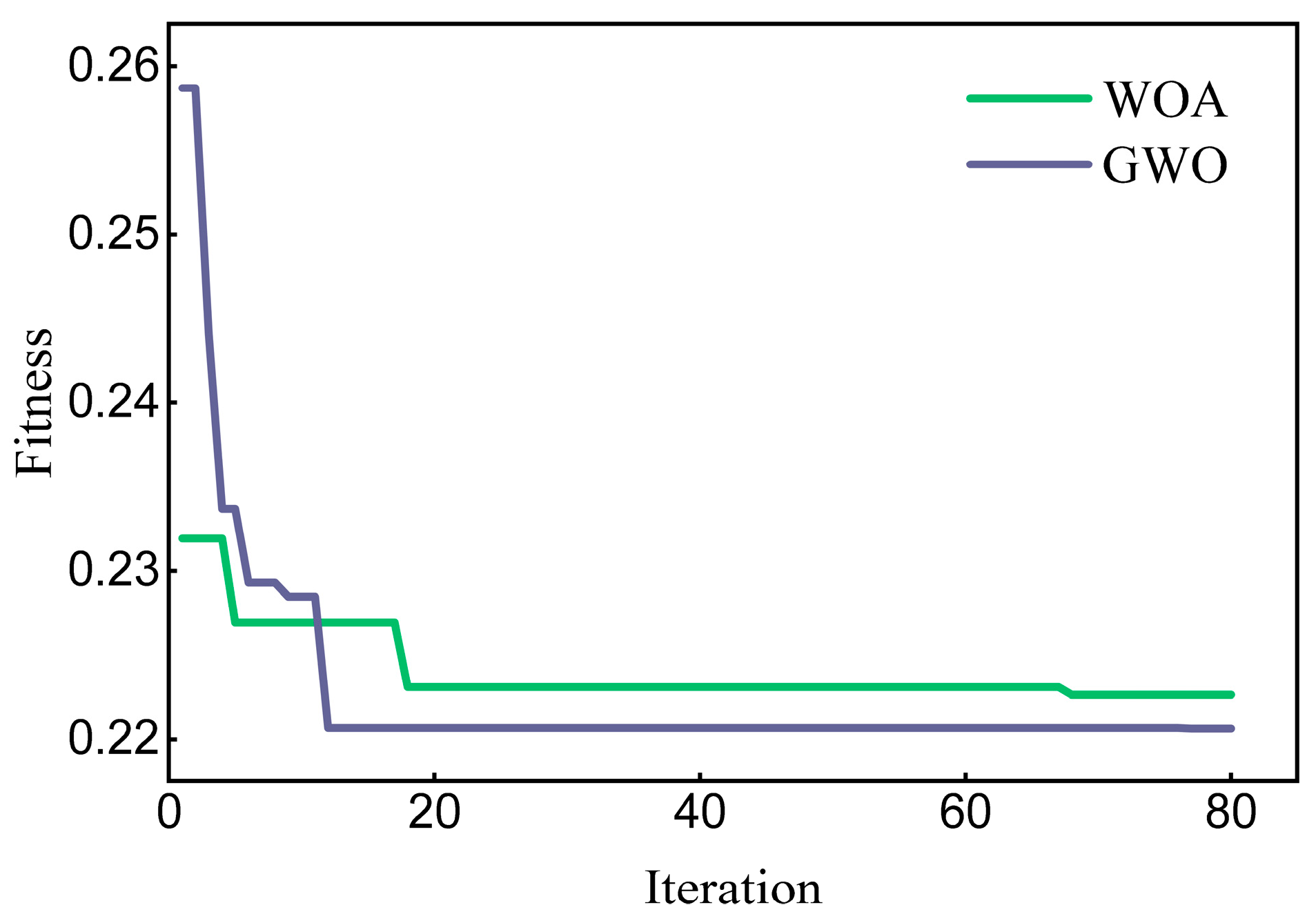
  • Intelligent optimization algorithms help the base model find suitable parameters, reduce the trial-and-error time, and improve the efficiency of model operation. In this study, the GWO algorithm has demonstrated superiority over WOA in finding the optimal parameters for LightGBM, leading to more accurate prediction outcomes in the experimental set up.
  • The residual term contains rich data signals, and decomposing the residual sequence can decompose the non-smooth, non-linear sequence into multiple regular subsequences, which in turn greatly improves the prediction degree of precision of the model. Compared to EEMD, CEEMDAN is more capable of decomposing residuals.
  • Suitable input feature indicators are crucial for model prediction. As the internet develops, people today increasingly tend to seek help online after becoming ill. Thus, the Baidu Index can provide abundant information about a certain disease.
Given that the Chinese National Influenza Center generally releases ILI% data several days after the deadline for reporting data with a certain lag, the combined model proposed in this study has strong applicability and is able to predict ILI% values one week in advance, which is of great relevance as it helps public health authorities make timely warnings about the risk of influenza transmission. While the model presented in this paper offers a high level of precision in forecasting trends of influenza trends, there are still aspects that require improvement.
  • Although multiple Baidu Index metrics influence the variability trends of influenza-like illness, it is inevitable in our research to subjectively select relevant Baidu Index metrics for analysis. However, in order to enhance objectivity and reliability in future studies, a more scientific and systematic approach to screening Baidu Index metrics can be explored in subsequent work, with the aim of refining the model and thereby providing more robust data support for influenza surveillance and early warning.
  • This study introduces a model that is specifically tailored for predicting the percentage of influenza-like illness in the southern region of China. However, the limitation in obtaining detailed data from individual provinces and cities within Southern China impeded our ability to accurately evaluate the model’s performance at these more granular geographical levels. Hence, the applicability of the model across specific regions in Southern China remains an open question for further investigation. Future research should concentrate on this issue to determine whether the model possesses predictive accuracy at more detailed regional levels.
  • Despite significant improvements with the proposed model, integrating GWO, LightGBM, and CEEMDAN, there is still ample room for further refinement. Future research endeavours could fruitfully investigate the incorporation of an ensemble learning strategy into the GWO-LightGBM model, followed by the application of a decomposition technique, to ascertain whether this approach can yield superior predictive outcomes.

Author Contributions

Conceptualization, Y.D. and C.L.; Data Curation, C.L.; Formal Analysis, Y.D.; Investigation, Y.G.; Methodology, C.L. and Y.G.; Software, X.W.; Validation, X.W. and H.W.; Visualization, X.W.; Writing—Original Draft, Y.D. and C.L.; Writing—Review and Editing, Y.D., C.L., Y.G. and H.W. All authors have read and agreed to the published version of the manuscript.

Funding

The authors are grateful for financial support from the National Natural Science Foundation of China (No. 81973791).

Data Availability Statement

In this study, ILI data were collected from the Influenza Weekly Report published on the Chinese National Influenza Center website (https://ivdc.chinacdc.cn/cnic/zyzx/, accessed on 25 February 2024), while Baidu Index data were obtained from the Baidu Index interface. The datasets used during this study are available from the corresponding author on reasonable request.

Conflicts of Interest

The authors declare no conflicts of interest.

References

  1. Krammer, F.; Smith, G.J.D.; Fouchier, R.A.M.; Peiris, M.; Kedzierska, K.; Doherty, P.C.; Palese, P.; Shaw, M.L.; Treanor, J.; Webster, R.G.; et al. Influenza. Nat. Rev. Dis. Primers 2018, 4, 3. [Google Scholar] [CrossRef]
  2. Li, H.; Ge, M.; Wang, C. Spatio-temporal evolution patterns of influenza incidence and its nonlinear spatial correlation with environmental pollutants in China. BMC Public Health 2023, 23, 1685. [Google Scholar] [CrossRef]
  3. Lei, H.; Yang, L.; Wang, G.; Zhang, C.; Xin, Y.; Sun, Q.; Zhang, B.; Chen, T.; Yang, J.; Huang, W.; et al. Transmission Patterns of Seasonal Influenza in China between 2010 and 2018. Viruses 2022, 14, 2063. [Google Scholar] [CrossRef]
  4. World Health Organization. Influenza (Seasonal). Available online: https://www.who.int/news-room/fact-sheets/detail/influenza- (accessed on 6 March 2024).
  5. Qian, C.; Dai, Q.G.; Xu, K.; Deng, F.; Huo, X. Application of the moving epidemic interval method in assessing the intensity of influenza epidemics in Jiangsu Province, China. Chin. J. Health Stat. 2020, 37, 10–13+17. [Google Scholar]
  6. Xue, H.; Zhang, L.; Liang, H.; Kuang, L.; Han, H.; Yang, X.; Guo, L. Influenza trend prediction method combining Baidu index and support vector regression based on an improved particle swarm optimization algorithm. AIMS Math 2023, 8, 25528–25549. [Google Scholar] [CrossRef]
  7. Amendolara, A.B.; Sant, D.; Rotstein, H.G.; Fortune, E. LSTM-based recurrent neural network provides effective short term flu forecasting. BMC Public Health 2023, 23, 1788. [Google Scholar] [CrossRef]
  8. Hu, X.; Hu, X.j. Comparative study of forecasting models for H1N1 influenza A epidemic in Xinjiang. Chin. J. Health Stat. 2011, 28, 342–343. [Google Scholar]
  9. Dai, H.; Zhou, N.; Ren, X.; Luo, P.; Yi, S.; Quan, M.; Zha, W.; Lv, Y. Epidemiologic characteristics and prediction of incidence trend of all types of influenza based on ARIMA model. Dis. Surveill. 2022, 37, 1338–1345. [Google Scholar]
  10. He, Z.; Tao, H. Epidemiology and ARIMA model of positive-rate of influenza viruses among children in Wuhan, China: A nine-year retrospective study. Int. J. Infect. Dis. 2018, 74, 61–70. [Google Scholar] [CrossRef] [PubMed]
  11. Chen, Y.; Leng, K.; Lu, Y.; Wen, L.; Qi, Y.; Gao, W.; Chen, H.; Bai, L.; An, X.; Sun, B.; et al. Epidemiological features and time-series analysis of influenza incidence in urban and rural areas of Shenyang, China, 2010–2018. Epidemiol. Infect. 2020, 148, e29. [Google Scholar] [CrossRef]
  12. Qian, C.S.; Jiang, C.Y.; Xia, H.; Zheng, Y.X.; Liu, X.H.; Yang, M.; Xia, T. Time series analysis and prediction modeling of the percentage of influenza-like illness visits in Shanghai, China. Shanghai J. Prev. Med. 2023, 35, 116–121. [Google Scholar]
  13. Qin, S.; Zhao, J.; Deng, P.; Zhang, Y.; Jiang, Y. Application of Joinpoint regression analysis in the trend of influenza incidence in Qinghai Province from 2005 to 2023. Chin. J. Dis. Control. Prev. 2024, 28, 1295–1300+1307. [Google Scholar] [CrossRef]
  14. Chen, Y.; Chu, C.W.; Chen, M.I.C.; Cook, A.R. The utility of LASSO-based models for real time forecasts of endemic infectious diseases: A cross country comparison. J. Biomed. Inform. 2018, 81, 16–30. [Google Scholar] [CrossRef]
  15. Signorini, A.; Segre, A.M.; Polgreen, P.M. The Use of Twitter to Track Levels of Disease Activity and Public Concern in the U.S. during the Influenza A H1N1 Pandemic. PLoS ONE 2011, 6, e19467. [Google Scholar] [CrossRef] [PubMed]
  16. Tsan, Y.-T.; Chen, D.-Y.; Liu, P.-Y.; Kristiani, E.; Nguyen, K.L.P.; Yang, C.-T. The Prediction of Influenza-like Illness and Respiratory Disease Using LSTM and ARIMA. Int. J. Environ. Res. Public Health 2022, 19, 1858. [Google Scholar] [CrossRef] [PubMed]
  17. Manohar, B.; Das, R. Artificial Neural Networks for the Prediction of Monkeypox Outbreak. Trop. Med. Infect. Dis. 2022, 7, 424. [Google Scholar] [CrossRef] [PubMed]
  18. Liu, C.L.; Hu, C.; Wang, P.; Hong, D.h.; Zhang, T.Z. Research on Multidimensional Credit Evaluation Model for Electricity Customers Based on Marketing Big Data. J. Southwest Univ. 2022, 44, 198–208. [Google Scholar] [CrossRef]
  19. Liang, Y.; Lin, Y.; Lu, Q. Forecasting gold price using a novel hybrid model with ICEEMDAN and LSTM-CNN-CBAM. Expert Syst. Appl. 2022, 206, 117847. [Google Scholar] [CrossRef]
  20. Liao, J.W. Research on Artificial Intelligence Forecasting of International Crude Oil Prices Based on VMD-LSTM-ELMAN Models. J. Chengdu Univ. Technol. 2024, 51, 164–180. [Google Scholar]
  21. Ginsberg, J.; Mohebbi, M.H.; Patel, R.S.; Brammer, L.; Smolinski, M.S.; Brilliant, L. Detecting influenza epidemics using search engine query data. Nature 2009, 457, 1012–1014. [Google Scholar] [CrossRef]
  22. Yuan, Q.; Nsoesie, E.O.; Lv, B.; Peng, G.; Chunara, R.; Brownstein, J.S. Monitoring Influenza Epidemics in China with Search Query from Baidu. PLoS ONE 2013, 8, e64323. [Google Scholar] [CrossRef]
  23. Li, Z.; Liu, T.; Zhu, G.; Lin, H.; Zhang, Y.; He, J.; Deng, A.; Peng, Z.; Xiao, J.; Rutherford, S.; et al. Dengue Baidu Search Index data can improve the prediction of local dengue epidemic: A case study in Guangzhou, China. PLoS Negl. Trop. Dis. 2017, 11, e0005354. [Google Scholar] [CrossRef] [PubMed]
  24. Wang, Y.; Zhou, H.; Zheng, L.; Li, M.; Hu, B. Using the Baidu index to predict trends in the incidence of tuberculosis in Jiangsu Province, China. Front. Public Health 2023, 11, 1203628. [Google Scholar] [CrossRef] [PubMed]
  25. Huang, R.; Luo, G.; Duan, Q.; Zhang, L.; Zhang, Q.; Tang, W.; Smith, M.K.; Li, J.; Zou, H. Using Baidu search index to monitor and predict newly diagnosed cases of HIV/AIDS, syphilis and gonorrhea in China: Estimates from a vector autoregressive (VAR) model. BMJ Open 2020, 10, e036098. [Google Scholar] [CrossRef] [PubMed]
  26. Dai, S.; Han, L. Influenza surveillance with Baidu index and attention-based long short-term memory model. PLoS ONE 2023, 18, e0280834. [Google Scholar] [CrossRef] [PubMed]
  27. Mestre, G.; Portela, J.; Rice, G.; Muñoz San Roque, A.; Alonso, E. Functional time series model identification and diagnosis by means of auto- and partial autocorrelation analysis. Comput. Stat. Data Anal. 2021, 155, 107108. [Google Scholar] [CrossRef]
  28. Gianfreda, A.; Maranzano, P.; Parisio, L.; Pelagatti, M. Testing for integration and cointegration when time series are observed with noise. Econ. Model. 2023, 125, 106352. [Google Scholar] [CrossRef]
  29. Duan, Y.; Zhang, J.; Wang, X.; Feng, M.; Ma, L. Forecasting carbon price using signal processing technology and extreme gradient boosting optimized by the whale optimization algorithm. Energy Sci Eng 2024, 12, 810–834. [Google Scholar] [CrossRef]
  30. Jiang, J.; Zhang, X.; Yuan, Z. Feature selection for classification with Spearman’s rank correlation coefficient-based self-information in divergence-based fuzzy rough sets. Expert Syst. Appl. 2024, 249, 123633. [Google Scholar] [CrossRef]
  31. Eden, S.K.; Li, C.; Shepherd, B.E. Nonparametric Estimation of Spearman’s Rank Correlation with Bivariate Survival Data. Biometrics 2022, 78, 421–434. [Google Scholar] [CrossRef] [PubMed]
  32. Zhong, M.X.; Xie, X.R. Clinical characterization of diabetic ketoacidosis combined with novel coronavirus pneumonia. Tianjin Med. J. 2023, 51, 1378–1381. [Google Scholar]
  33. Mirjalili, S.; Mirjalili, S.M.; Lewis, A. Grey Wolf Optimizer. Adv. Eng. Softw. 2014, 69, 46–61. [Google Scholar] [CrossRef]
  34. Ke, G.; Meng, Q.; Finley, T.; Wang, T.; Chen, W.; Ma, W.; Ye, Q.; Liu, T.-Y. LightGBM: A highly efficient gradient boosting decision tree. In Proceedings of the 31st International Conference on Neural Information Processing Systems, Long Beach, CA, USA, 4 December 2017; pp. 3149–3157. [Google Scholar]
  35. Friedman, J.H. Greedy function approximation: A gradient boosting machine. Ann Statist 2001, 29, 1189–1232. [Google Scholar] [CrossRef]
  36. Torres, M.E.; Colominas, M.A.; Schlotthauer, G.; Flandrin, P. A complete ensemble empirical mode decomposition with adaptive noise. In Proceedings of the 2011 IEEE International Conference on Acoustics, Speech and Signal Processing (ICASSP), Prague, Czech Republic, 22–27 May 2011; pp. 4144–4147. [Google Scholar]
  37. Cai, X.; Li, D.; Feng, L. Enhanced Carbon Price Forecasting Using Extended Sliding Window Decomposition with LSTM and SVR. Mathematics 2024, 12, 3713. [Google Scholar] [CrossRef]
  38. Hodson, T.O. Root-mean-square error (RMSE) or mean absolute error (MAE): When to use them or not. Geosci. Model Dev. 2022, 15, 5481–5487. [Google Scholar] [CrossRef]
  39. Zhang, X.-x.; Gu, L.-l.; Chen, H.; Jia, G.-z. Study on the influence of surrounding urban SO, NO, and CO on haze formation in Beijing based on MF-DCCA and boosting algorithms. Concurr. Comput. Pract. Exp. 2020, 32, e5921. [Google Scholar] [CrossRef]
  40. Chicco, D.; Warrens, M.J.; Jurman, G. The coefficient of determination R-squared is more informative than SMAPE, MAE, MAPE, MSE and RMSE in regression analysis evaluation. PeerJ Comput. Sci. 2021, 7, e623. [Google Scholar] [CrossRef] [PubMed]
  41. Shaik, N.B.; Jongkittinarukorn, K.; Bingi, K. XGBoost based enhanced predictive model for handling missing input parameters: A case study on gas turbine. Case Stud. Chem. Environ. Eng. 2024, 10, 100775. [Google Scholar] [CrossRef]
  42. Ihssan, S.; Shaik, N.B.; Belouaggadia, N.; Jammoukh, M.; Nasserddine, A. Enhancing PEHD pipes reliability prediction: Integrating ANN and FEM for tensile strength analysis. Appl. Surf. Sci. Adv. 2024, 23, 100630. [Google Scholar] [CrossRef]
  43. Tian, L.; Feng, L.; Yang, L.; Guo, Y. Stock price prediction based on LSTM and LightGBM hybrid model. J. Supercomput. 2022, 78, 11768–11793. [Google Scholar] [CrossRef]
  44. Guo, J.; Yun, S.; Meng, Y.; He, N.; Ye, D.; Zhao, Z.; Jia, L.; Yang, L. Prediction of heating and cooling loads based on light gradient boosting machine algorithms. Build. Environ. 2023, 236, 110252. [Google Scholar] [CrossRef]
  45. Duan, Y.; Zhang, J.; Wang, X. Henry Hub monthly natural gas price forecasting using CEEMDAN–Bagging–HHO–SVR. Front. Energy Res. 2023, 11, 1323073. [Google Scholar] [CrossRef]
Figure 1. ILI% in Southern China from 2019 to 2023.
Mathematics 13 00024 g001
Figure 2. The PACF results of ILI%.
Mathematics 13 00024 g002
Figure 3. Framework of ILI% prediction based on GWO-LightGBM-CEEMDAN.
Mathematics 13 00024 g003
Figure 4. Fitness function convergence curves of WOA and GWO.
Mathematics 13 00024 g004
Figure 5. CEEMDAN decomposition result for residual.
Mathematics 13 00024 g005
Figure 6. Performance of different models.
Mathematics 13 00024 g006
Figure 7. Forecasting results of each model. (a) RMSE, MAE, MAPE; (b) R2.
Mathematics 13 00024 g007
Table 1. Descriptive statistics of experimental data.
CountMeanStdMin25%50%75%Max
Training set2093.7511.2812.2003.0003.5004.00013.000
Testing set525.7062.3351.4004.2755.4507.12510.100
Table 2. Baidu Index classification.
CategoryKeywords
Common wordsCold(X1), influenza(X2), A influenza(X3), B influenza(X4), virus infection(X5), respiratory tract infection(X6), influenza virus(X7)
PreventionPrevent the flu(X8), vaccination(X9), influenza vaccine(X10), mask(X11), alcohol(X12), disinfectant(X13), hand sanitizer(X14)
SymptomsFever(X15), high fever(X16), headache(X17), sore throat(X18), run at the nose(X19), sneeze(X20), nasal obstruction(X21), cough(X22), bronchitis(X23), diarrhea(X24), white lung(X25), leucocyte(X26), lymphocyte(X27)
TreatmentNebulizer(X28), febrifuge(X29), ibuprofen(X30), Kuaike cold medication(X31), GanKang cold medication(X32), Tylenol(X33), oseltamivir(X34), ribavirin(X35), Suhuang Zhike Capsule(X36), antiviral oral liquid(X37)
Table 3. ADF test of ILI%.
VariableDifference Ordertp-Value1%5%10%
ILI%0−4.170.001−3.456−2.873−2.573
1−8.770.000−3.457−2.873−2.573
Table 4. Spearman correlation of each index.
VariableCorrelation Coefficientp-ValueVariableCorrelation Coefficientp-Value
X10.4220.000X200.0390.532
X20.4040.000X210.1480.017
X30.7240.000X220.4500.000
X40.6740.000X230.5670.000
X50.6420.000X24−0.0340.585
X60.6770.000X250.3490.000
X70.3220.000X260.0090.880
X80.4160.000X270.2920.000
X9−0.3680.000X280.5640.000
X100.0880.155X290.6750.000
X11−0.3890.000X300.4320.000
X12−0.2740.000X310.4550.000
X13−0.3810.000X320.4950.000
X14−0.2590.000X330.5640.000
X150.7210.000X340.7500.000
X160.6420.000X350.6500.000
X17−0.0670.278X360.5580.000
X180.4800.000X370.7050.000
X190.2380.000
Table 5. Parameters setting of related algorithms.
Algorithm NameParameters Setting
XGBoostDefault
LightGBMDefault
WOA-LightGBMIterations = 30; noposs = 20;
n_estimators = 38; num_leaves = 19; learning_rate = 0.082047; max_depth = 6
GWO-LightGBMIterations = 30; noposs = 20;
n_estimators = 10; num_leaves = 9; learning_rate = 0.020407; max_depth = 6
Table 6. Characteristics of different models.
ModelsParameter OptimizationDecomposition Technique
XGBoost (Model 1)
LightGBM (Model 2)
WOA-LightGBM (Model 3)
GWO-LightGBM (Model 4)
GWO-LightGBM-EEMD (Model 5)
GWO-LightGBM-CEEMDAN (Model 6)
Table 7. Evaluation indicators. Optimal values given in bold.
ModelsRMSEMAEMAPER2
XGBoost0.3375390.3211386.0247220.978697
LightGBM0.3290140.3097345.7079690.979760
WOA-LightGBM0.3091580.2941245.4744320.982129
GWO-LightGBM0.2218160.2210444.6849170.990800
GWO-LightGBM-EEMD0.0125360.0109020.2249600.999971
GWO-LightGBM-CEEMDAN0.0106880.0079810.1979240.999979
Table 8. Comparison between proposed model and contrast model. Optimal values given in bold.
ModelRMSEMAEMAPER2
GWO-LightGBM-CEEMDAN (Model 6)0.0106880.0079810.1979240.999979
GWO-LightGBM-CEEMDAN’ (Model 7)0.0126960.0100010.2139150.999970
Table 9. The improvement percentage of the models.
Benchmark Model Comparative ModelRMSEMAEMAPE
1LightGBMVS.GWO-LightGBM32.58%28.63%17.92%
2GWO-LightGBMVS.GWO-LightGBM-EEMD94.35%95.07%95.20%
3GWO-LightGBM-EEMDVS.GWO-LightGBM-CEEMDAN14.74%26.79%12.02%
4GWO-LightGBM-CEEMDAN’VS.GWO-LightGBM-CEEMDAN15.82%20.20%7.48%
Disclaimer/Publisher’s Note: The statements, opinions and data contained in all publications are solely those of the individual author(s) and contributor(s) and not of MDPI and/or the editor(s). MDPI and/or the editor(s) disclaim responsibility for any injury to people or property resulting from any ideas, methods, instructions or products referred to in the content.

