Abstract
The evaluation of low-degree hypergeometric polynomials to zero defines algebraic hypersurfaces in the affine space of the free parameters and the argument of the hypergeometric function. This article investigates the algebraic surfaces defined by the hypergeometric equation with or . As a captivating application, these surfaces parametrize certain families of genus 0 Belyi maps. Thereby, this article contributes to the systematic enumeration of Belyi maps.
MSC:
33C05; 57M12; 14J27
1. Introduction
The systematic cataloging of Belyi maps is an active research undertaking [1,2,3]. Contributing to this venture, this article considers comprehensively Belyi maps of the form
or
where is a polynomial of degree m without multiple roots, and
asymptotically. This implies . The powers are allowed to be positive or negative integers, and they are assumed to be different. If the powers are positive integers, then is a polynomial. Recall that polynomial Belyi maps are called Shabat polynomials ([4] §2.2) or generalized Chebyshev polynomials [5]. We are particularly interested in Belyi maps defined over .
Assuming that the point is above , the distinct points in the three canonical fibers are as follows:
- Two roots of or , of branching order or , above or depending on the signs of ;
- The roots of , of branching order , above ;
- The point , of branching order or , respectively, for the two forms, above ;
- The point , of branching order , above ;
- non-branching points above , where d is the degree of .
In total, we count
distinct points in the three fibers, which is the minimal number of points in three fibers for a covering by the Riemann–Hurwitz formula ([6] Theorem 5.9), and the number of points that Belyi maps of genus 0 must have in the three fibers. This will be recapped in Lemma 3.
As it turns out, the considered families of Belyi maps are parametrized by the zero sets of hypergeometric polynomial equations, namely
for the Belyi maps of the form (1), and
for the form (2). These hypergeometric equations were derived earlier by Adrianov ([5] Propositions 3.5, 3.8) in the context of Shabat polynomials. The equations give the generic number of distinct Belyi maps (up to Möbius transformations) of the considered branching patterns, namely, for fixed in the form (1), or for fixed in the form (2). As we show in Lemmas 1 and 2, this number is smaller when one of the quotients , is a larger negative integer. It appears that the hypergeometric polynomials in (5), (6) are irreducible over typically, giving the maximal Galois orbits of Belyi maps with the considered branching patterns.
The considered Belyi maps constitute a borderline easy case that continues extensively the examples in ([4] §2.2) and [7]. The new examples and methodology will not be radically novel for active readers of [4,7]. In particular, we encounter new families of Belyi maps defined over that are parametrized by the following:
- Rational points on an elliptic curve, as in ([4] §2.2.4.3); see Examples 8, 13 and 14 here.
- Integer solutions of Pell’s equation, as in ([7] Ch. 10); see Example 18.
- Rational points on a cubic surface or a cubic pencil; see Examples 4, 5.
- Integral points on elliptic curves or elliptic surfaces; see Example 9.
The investigation of this article starts with recalling the relevant properties of hypergeometric functions. Section 2 introduces the hypergeometric -function, the Pochhammer symbol , and the key properties of hypergeometric polynomials that we use. Section 3 and Section 4 consider the algebraic surfaces defined by the equation
with or . We modify the lower parameter to , so that after clearing the denominators, we have the symmetric identity
of the same hypergeometric summation in the opposite directions. The parameters are, thereby, interchangeable in combination with the Möbius transformation . These equations with define algebraic surfaces in the affine space defined by the parameters as coordinates. Further symmetries of these hypergeometric polynomials are presented in (11)–(14).
The technical contribution of this article is the careful consideration of the hypergeometric polynomial equations, including their degenerations, and analysis of their algebraic structure and elliptic fibrations. The algebraic surfaces defined by the cubic or quartic Equation (7) are investigated in Section 3 and Section 4, respectively. As Belyi maps are defined for and (but preferably for us, ), we are particularly interested in the rational points and elliptic fibrations on these algebraic surfaces.
The later sections describe the Belyi maps of the forms (1) and (2). Section 5 presents the easy examples of Belyi maps that the considered two forms generalize. These easy examples are largely covered in ([4] §2.2). Section 6 considers Belyi maps of the form (1) using rational parametrizations of the examined surfaces (7). The cases with fewer than N Belyi maps in Examples 8 and 9 are parametrized by particular elliptic curves on the same surfaces. Section 7 considers Belyi maps of the form (2). This leads to considering rational or integral points on some other elliptic curves on the same surfaces. Our thorough investigation of algebraic surfaces (7) allows to refine the examples in ([4] §2.2.4.3) and ([7] Ch. 10), and to explore beyond them.
2. Hypergeometric Details
The Gauss hypergeometric function ([8] Ch. 2) is defined by the series
Here, denotes the Pochhammer symbol, or the “raising” variant of the factorial. Using the -function ([8] Ch. 1) we can write
The standard analytic continuation of the -function is onto . This function is undefined when c equals zero or a negative integer.
2.1. Hypergeometric Polynomials
If well defined, the hypergeometric series (9) is a polynomial in z when a or b are non-positive integers. In addition to (8), we have these symmetries of hypergeometric polynomials:
where . The following expression defines a polynomial of degree for any integer :
If c is a non-negative integer but a or b is a non-negative integer , the hypergeometric summation (9) can be considered a polynomial of degree or . This interpretation is often used in theory of orthogonal polynomials [9]. We adopt this interpretation of hypergeometric functions like
with integer . The well-known identities
of Pfaff and Euler ([8] Th. 2.2.5) should not be automatically applied then; see ([10] Lemma 3.1). Yet these identities are valid when all three numbers are non-negative integers, and ; see ([10] §9).
2.2. Distinctive Roots of Hypergeometric Polynomials
The distinctiveness of the roots of hypergeometric polynomials is easily proved by using contiguous relations ([8] §2.5, §3.7) of -functions. In particular, we use the observations in the following two lemmas. Complementarily, one may consider the relation of hypergeometric polynomials to classical orthogonal polynomials [9] and the interlacing properties of the zeroes of orthogonal polynomials ([8] §5.4).
Lemma 1.
Consider the sequence of hypergeometric polynomials
with some . Suppose that for a positive integer k, we have , , and . Then, we have the following:
- (i)
- The polynomials and do not have common roots.
- (ii)
- The polynomial has k distinct roots.
- (iii)
- is not a root of .
Proof.
The sequence satisfies the recurrence relation
This follows from the contiguous relations [11], or by applying Zeilberger’s algorithm ([8] §3.11), or by checking the series expansion. We apply the recurrence with decreasing k, and use the assumption that . The recurrence implies that a common root of and is either , which conflicts with the hypergeometric values 1 at , or it would be a common root of , and of contradictorily.
The second statement follows from the degree of k of thanks to , and the fact that another contiguous relation
implies that a multiple root of would be also a root of , leading to the established first statement.
The last statement follows from the Chu–Vandermonde identity ([8] p. 67)
giving the value for evaluated at . □
Lemma 2.
Consider the sequence of hypergeometric polynomials
with some . Suppose that for a positive integer k we have and . Then, we have the following:
- (i)
- The polynomials and do not have common roots.
- (ii)
- The polynomial has distinct roots.
- (iii)
- is not a root of .
Proof.
The sequence satisfies the recurrence relation
Under the assumption that , the recurrence shows that a common root of and is either the rejectable , or it would be a common root of , , and of contradictorily.
The second statement follows from the degree of k of , thanks to , and the fact that another contiguous relation
implies that a multiple root of would be also a root of , leading to the established first statement.
The last statement follows from applying the Chu–Vandermonde identity (22). The evaluation at is
for both even and odd k. □
3. Cubic Hypergeometric Polynomials
After clearing the denominators in the equation , we obtain
or rather more compactly,
Let denote the algebraic surface defined by (27), of degree 6.
Fixing z leads to a cubic equation in . For , the equation factorizes into three linear factors. For , it factorizes into quadratic and linear parts. For other fixed z, we obtain an irreducible cubic curve of genus 0. Here is a parametrization of those cubic curves by :
This also gives a birational parametrization of by z and e. If in the denominators, then the polynomial in (27) can be factored as
Both numerators in (29) equal 0 as well at the exceptional three points . The three points are blown up to these lines on :
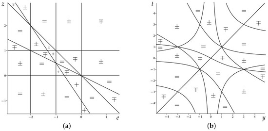
We are interested in the points on with both being positive, while and . The dependence of the signs of on the parameters by the parametrization (29) is depicted in Figure 1a. There are two regions marked by + where b and c are positive; they are delineated by
The exceptional lines (30) do not apply to this interest.
3.1. Complete Factorization for Some
Suppose that the parameters have the form (29) for some and . Considering (27) as a cubic polynomial in z, it then has the root . For generic values of , the other two roots solve the quadratic equation
We are interested when those other roots are in as well. For that, the discriminant
must be a full square. We apply the birational transformation
and the discriminant becomes
The values should therefore determine a -rational point on the cubic surface
This cubic surface has three singularities . By intersecting this surface with the pencil of lines , through the singularity , we obtain this birational parametrization by :
This translates to
and ultimately to
This parametrizes the cases when the cubic polynomial (27) factors completely. The special case gives the following neat family:
The algebraic map (39) is 2-to-1 generically, as the central symmetry keeps invariant and permutes the roots of (33). Up to this symmetry, the inverse map to (39) is
There is no point where both b and c are positive by the parametrization (40); see Figure 1b, and note that the only points where both are undetermined by (40) give in (39) and hence are rejectable in (29).
3.2. Elliptic Fibration by b or c
For fixed , Equation (27) defines a cubic curve of genus 1. Its j-invariant equals
We can consider as an elliptic surface ([12] III.11) over . We are interested in its basic -arithmetic properties [6,12]. The following propositions give an isomorphic Weierstrass form for the elliptic surface, and a characterization of rational curves on it in terms of the Mordell–Weil group.
Proposition 1.
Proof.
It is straightforward to check the isomorphism (46). The inverse map is given as
As a side note, the elliptic involution corresponds to the hypergeometric symmetry (11) under this isomorphism.
The canonical Weierstrass form can be obtained by applying the shift in (45). The discriminant ([12] III.1) of the elliptic surface equals . By considering and the j-invariant in (44), we can use ([13] Table 5.1) and conclude that the singular fibers have the Kodaira types IV, I3, I2, I3, respectively. By [13] (Fig. 5.1–5.2), they have, respectively, irreducible components in the Kodaira–Neron model. By the Shioda–Tate formula ([13] Corollary 6.7), the Mordell–Weil rank equals , as the Neron–Severi rank is 10 for rational elliptic surfaces ([13] §7.2). By [13] (Theorem 8.33), the Mordell–Weil group is generated by polynomial points with , . Direct computation with undetermined coefficients gives eight possibilities for such u:
The points with are flex points with the tangents ; hence, they are 3-torsion points. An investigation of the group relations between all candidate points shows that we can take a point with , , for a free generator. □
Taking in (45) gives an elliptic curve over , with the same Mordell–Weil group typically ([12] III.11). But the Mordell–Weil group group over could be larger than the projected set of points from the elliptic surface. For example, gives the Mordell–Weil group , as we will consider in Example 8.
It is instructive to consider several of the simplest sections on , parametrized by b, and map them to the original surface defined by (27). Here are a few obtained non-degenerate c-values of low degree in b:
After substituting these values into (27), there is a linear factor in z. That parametrizes fully the corresponding section in on .
If we have a root described by (46) of the cubic hypergeometric polynomial with fixed c (and possibly b), the other two roots are equal to
To seek the rationality of these roots, we may replace and obtain a family of hyperelliptic curves of genus 2. One may go through a limited list of Mordell–Weil points on (be it specialized, with for example) and check that apparently, the complete factorization of the cubic polynomial happens generically only in degenerate cases such as . We need b to be expressible as in (40). The family (41) corresponds to the infinite point on the elliptic surface.
4. Quartic Hypergeometric Polynomials
A compact polynomial form of the equation is
Let us denote this surface by . We will associate two elliptic surfaces and to it.
4.1. Elliptic Fibration by z
For fixed z, the curve has genus 1 generically. We identify directly as an elliptic surface. As such, it is isomorphic to
where . The j-invariant is rather untidy in the denominator:
An isomorphism is given by
with
where
The infinite point on (52) is mapped to the central point among the degenerations. The parametric expression for simplifies to
As we consider in the next subsection, is a rational elliptic surface. Its Mordell–Weil group has no torsion, and the maximal rank 8 for elliptic surfaces over , as is evident ([13] §7.3) from the irreducible degree 12 denominator of the j-invariant (53), meaning that the surface has 12 singular fibers of Kodaira type . By [13] (Theorem 7.12 (i)), there are 240 candidate points with a polynomial coordinate of degree to generate the Mordell–Weil group. Computations show that 60 of them are defined over . They have
or can be obtained by further applying the hypergeometric symmetries (8), (11)–(14), generated by and . Further, the two points with are defined over , and the points with are defined over . Additionally, 64 points have , 64 points have , and 48 points have . The Mordell–Weil group over has rank 6. It is generated by points with . Examples of simpler rational sections on the original surface (51) have these non-degenerate values of b:
The corresponding -coordinate is obtained from a linear factor of (51) that arises after substituting b. Due to the hypergeometric symmetry (8), some possible values for c can be obtained by substituting in (59).
4.2. The Rational Surface
The discriminant of the elliptic surface (52) is of degree 12 in z; see the denominator of (53). Therefore, it is a rational surface ([13] §7.5) that can be obtained from a pencil of cubic curves in (linearly parametrized by z) by blowing up the nine intersection points of the pencil. Rather equivalently [14], it is a del Pezzo surface in the weighted projective space with weights , of degree 1.
The surface is birational to the elliptic surface (52) in the Weierstrass form; hence, it can also be obtained from the pencil of cubic curves in . To obtain a rational parametrization of , we first notice the simpler defining equation
in the coordinates
The new equation defines a del Pezzo surface in the weighted projective space with weights , of degree 2. It contains four lines in the hyperplane . Choosing the line to blow down, we apply a standard step (called unprojection in ([14] §5)) in resolving del Pezzo surfaces by introducing the coordinate
We can eliminate f straightaway and obtain the following non-singular cubic surface in :
Subsequently, we can blow down one of the lines on the plane , or apply a classical parametrization recipe ([13] §10.5.3) using two skew lines on the cubic surface, say, and . Eventually, a suitable simplified cubic pencil is defined by , where
A parametrization of is given by and
The inverse map is given by
Computations with two versions of in (64)–(66) show that the hypergeometric symmetries (8), (11)–(14) are realized by non-linear Cremona [15] transformations of the parameters . For example, (8) is realized by
while (11) is realized by
4.3. The Fibration by b
Equation (51) with fixed b defines a quartic curve of the generic genus 3. We can reduce the genus to 1 by factoring out the hypergeometric symmetry (11). This gives an elliptic surface isomorphic to
The symmetry invariants are parametrized as follows:
where . The inverse projection is given by
Rational points on the quartic curves can be found by trying to lift from the rational fibers on the elliptic surface. Its Mordell–Weil group can be determined similarly to the proof of Proposition 1. The discriminant of the elliptic surface equals , and the j-invariant equals
Using ([13] Table 5.1), we conclude that the singular fibers have the Kodaira types III, I4, I2, I3, respectively. They have, respectively, irreducible components. The Mordell–Weil rank equals . The candidates for the generators have
The Mordell–Weil group is isomorphic to . The group is generated by the 2-torsion point and a point having . The point
can be taken as a free generator.
The discriminant of the quadratic Equation (73) for z equals
on . To find rational sections on the genus 3 curve, we need the denominator
to be a full square on . The point leads to
A rational section is obtained after the base change .
5. Belyi Maps
Recall that Belyi maps are algebraic coverings that branch in the three fibers . We consider Belyi of genus 0 only. The following characteristic property of Belyi maps of genus 0 follows from the Riemann–Hurwitz formula.
Lemma 3.
A Belyi map of genus 0 and degree d has exactly distinct points in the 3 fibers .
As summed up in (4), the considered maps (1) and (2) satisfy the condition of this lemma. The degree of (1) equals
while the degree of (2) equals . Without loss of generality, we may assume .
Easy Maps
The simplest Belyi maps are the power functions . They have just two points in the two fibers and . Our considered rational maps can be viewed as a close neighborhood of this exemplar in the landscape of Belyi maps.
Example 1.
The Belyi maps with exactly three points in two fibers are easy to find; see [7] §6.6.2 with . These maps necessarily have two points with some branching orders in one fiber (say, ) and one point (say, ) of branching order in the other fiber (say, ). There must be then distinct points in the third fiber by Lemma 3; hence, there, we have exactly one branching point, of order two. The most compact expression for the Belyi map is obtained after choosing this branching point to be :
This form matches the case , of (1), where we take to be positive, and rescale .
Example 2.
Consider Belyi maps of the more general form
where is a polynomial or degree m, as in [7] §6.6.2. If are positive integers, then these maps have one point of order p, m points of order q above , a single point of order above , and a branching point of order above . The other points above are non-branching by Lemma 3. By the equality of (86) and (87), we have
This means that the polynomial equals the truncated Taylor series of at . Explicitly,
Following our interpretation of hypergeometric polynomials (16), we can write
Remark 1.
Remark 2.
If we take or , then we have (rather than ) points in the two fibers . The branching order of can be at most m then, and (88) should be modified to . We obtain the Belyi maps , after scaling x additionally.
Example 3.
Now we look at the Belyi maps of the form
with . This is the case of (1). The series expansion of (91) starts with
The coefficients to must vanish. Eliminating λ, we obtain a quadratic equation for μ. Its discriminant equals ; hence, the Belyi maps are expressed with the radical . Explicitly,
These Belyi maps with the definition field are obtained in [4] (Example 2.2.25). If are positive integers, the definition field is an imaginary quadratic extension of . But the Belyi maps could be defined over if both positive and negative powers are prescribed. For example, here is a nice family of paired Belyi maps with , , :
A general rational parametrization of the triples with is obtained by parametrizing the singular cubic surface , identifying , . Here is such a parametrization by , , up to the simultaneous scaling of :
Then, . After rescaling x in the two forthcoming Belyi maps, we obtain the expressions
which are to be raised to a common power so as to make the three powers integral. The cases with fall outside the considered shape (91), and the cases with coalescing branching points require special attention. In the latter situation, we have .
Remark 3.
If in the last example, then . Taking gives the trivial function . Taking gives
In the cases or , we also have just one Belyi map analogously. If simultaneously , both candidate functions collapse to .
6. Belyi Maps of the Form (1)
Belyi maps of the shape (1) generalize Example 3 from . We assume that the numbers are non-zero such that there are indeed distinct points above and . The points , , and their branching orders p, q, are permutable. We also assume , , , as these cases are considered in Section 7 with the smallest field of definition.
The condition (3) translates into the power series relation
The power series term with has to equal 0 then. The polynomial is determined uniquely by the power series
truncated at the -th term.
Proof.
The left-hand side of (100) is the polynomial under the stated conditions. When , the polynomial is forced to be of a smaller degree than m. If , then has the undue roots , . □
The coefficients in (100) can be expressed as follows:
or
We must have , which leads to Equation (5), generically.
6.1. Full Sets of Belyi Maps
Here we consider examples of the generic case (104) with Belyi maps. We are interested in the cases and . The degenerate value would coalesce the points of branching order p and q, but this point is excluded by Lemma 1 (iii). By Lemma 1 (ii), the hypergeometric polynomial has distinct roots when
The condition is equivalent to
underscoring the symmetry of the branching orders p, q, and .
The following examples investigate the Belyi maps with and . The case is considered in Example 3.
Example 4.
In the case , we consider Equation (27) specialized by , , :
The discriminant
is proportional to , and it indeed vanishes only when we have fewer than three distinct roots, and those roots as in Lemma 1 .
Belyi maps defined over can be found using the parametrization (29), identifying , , and . Polynomial Belyi maps defined over are obtained from the + regions (32) in Figure 1a. For example, and produce these Shabat polynomials, respectively:
Their companions with the same are defined, respectively, over and . There are no triples of Shabat polynomials defined over , as there is no point giving positive values for and by Figure 1b. The family (41) with provides most of the triples of Belyi maps defined over with small absolute values of . For example, gives the case with these three Belyi maps defined over :
Here are a few projective ratios giving three Belyi maps defined over outside the family (41):
Families of Belyi maps can be obtained from sections on the elliptic surface , particularly from the c-values in (48). Taking with the reparametrization and independent rescaling of x and of the powers gives
Similarly, taking and gives
Or one may employ the whole two-parameter uniformizations (29) or (41).
Example 5.
Similarly, for , we obtain the surface in (51) with , , . We can use the full parametrization (66) and (67), or a section of the elliptic surface in (52). For example, the first b-value from (59) gives the family
with . Here are some values of , with one of them being a positive integer, found by an extensive search through the parametrization (66):
The negative integer values of are considered in Example 9. Here are some other found values of , excluding the values with reference to Examples 15 and 16:
6.2. Cases with Fewer Belyi Maps
The number of Belyi maps (1) with is smaller than when at least one of the conditions (104) is not satisfied. Indeed, if for a positive integer , the polynomial has the degree ℓ rather than , as the terms with in (101) vanish then. If for a positive integer , then the first terms in (101) vanish, and
The factor reduces the number of relevant roots to ℓ. If for a positive integer but and , then we apply Euler’s transformation (18) to the hypergeometric polynomial and obtain
The factor reduces the number of relevant roots to . If and , then these possibilities may combine, giving a lower degree of and multiple undue roots and . Figure 2 depicts the regions and line segments or rays on the integer lattice for the values of and where the number of Belyi maps (1) is fixed . Lemma 4 applies to the visible triangle inside the dark middle region.
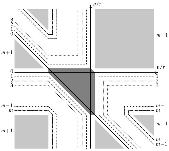
Figure 2.
The number of Belyi maps (1) for integer values of and . The dark region in the middle, and the lines emanating from it, represent the cases with no Belyi maps. The light grey regions represent Belyi maps; the dashed lines—unique Belyi maps; the dense dotted lines—pairs of Belyi maps; the sparser dotted lines—triples of maps; the two kinds of dashed–dotted lines: or m maps.
Let us consider the cases of reduced sets of distinct Belyi maps of size at most 4. Let us use and for shorthand.
Example 6.
The cases of single Belyi maps are represented by some lattice points on the lines , , or , , in Figure 2. It is enough to consider two cases, that is, one from both displayed triples of lines, due to the hypergeometric symmetries (8), (11)–(14). When and , the hypergeometric polynomial is linear in λ. It gives . Following (99), consider the power series
The term with indeed vanishes, and the earlier terms define .
When and , then (115) reads
The hypergeometric polynomial on the right-hand side is linear, and gives . The implication for the power series of
is remarkable: the k-th term is divisible by when . Here is a revealing form of the starting terms:
Example 7.
Here, we consider the cases with two Belyi maps. They are represented by some lattice points on the lines , , and or , , and in Figure 2. It is enough to consider two cases. When and , the hypergeometric polynomial is quadratic in λ:
The two solutions are
We have two Belyi maps that are defined over when
for some . Then, the λ-values are . The power series then looks like this:
Note that if then , and we have just one Belyi map with , which is a special case of (118).
Example 8.
Now we consider the cases with larger m that have three Belyi maps. Suppose that . Then, the hypergeometric polynomial (114) for defines a cubic relation between λ and . This cubic relation defines a curve of genus 1 as stated in Proposition 1. The elliptic curve has the Mordell–Weil group isomorphic to for general m. The isomorphism (46) has to be adjusted with
Analysis with the database [16] found the examples with giving the Mordell–Weil group , though the cases are not in the database yet. In particular, the elliptic curve for the case has the label 39690.bj2 in [16]. The equation specialized from (45) is
Besides the specialized generators and of Proposition 1, its Mordell–Weil group has also the generator over . This extra generator corresponds to the hypergeometric evaluation
and the Belyi map
It is interesting to observe that the expanded polynomial does not have the terms with (as we just used) and with , . Therefore, we can obtain two more Belyi maps by extending the numerator of (129) to polynomials of degree or . This phenomenon is typical for integer points on our hypergeometric surfaces as the next example suggests.
Example 9.
Here we look at the cases with larger m that have four Belyi maps. For , the parametrization (66) and (67) has to be adjusted by (126). We seek negative values of b or due to the hypergeometric symmetries (8), (11)–(14). Here are some cases for being found:
Of particular interest are the points with both negative integers. Found instances are
They give two Belyi maps though for different cases of . For example, the first instance gives the hypergeometric evaluations
They both lead to consider the polynomial
as a power series without the terms or .
Remark 4.
The cases like (128), (132) of hypergeometric equations with integer parameters can be expressed in terms of Krawtchouk polynomials ([9] §9.11):
Following (11), hypergeometric polynomials in (128), (132) are identified by
Finding the integer roots of Krawtchouk polynomials is an active field of research ([17,18] §7.2) with special implications for graph and coding theories [19], algebraic geometry [20], Padé approximations ([21] §2.2), and quantum entanglement [22].
7. Belyi Maps of the Form (2)
The form (2) of Belyi maps is the compacted case of the form (1), where is replaced by the aggregate power . This grouping of points with the same branching order is routinely used to maximally simplify the field of definition of Belyi maps [4]. Similarly, here we are not interested in the case . These maps correspond to the cases of Remark 2, with a quadratic factor of separated.
Let us denote . The condition (3) translates into the power series relation
The power series term with has to equal 0. The polynomial is determined uniquely by the power series
truncated at the -the term. The power series of can be computed by expanding in
Explicitly,
If and , we have the hypergeometric expression
Distinct Belyi maps correspond to the roots of , identified up to the -weighted homogeneous action of scaling x. There is a Belyi map with when m is even. It is obtained from Example 2 after the substitution , (with over there equal to the current ).
The following degeneratated cases are encountered:
- There are no Belyi maps when for a positive integer because then , and possibly of lesser degree than m.
- If for a positive integer satisfying , then the first terms for the sum (139) for are zero, and has the degenerate root of that multiplicity. After shifting the summation index by ,There are proper Belyi maps then, including the case for even m.
- If for a positive odd integer , thenby Euler’s Formula (18). The root corresponds to the degeneration of to a full square. The transformed hypergeometric sum can be identified as with the substituted . There are then Belyi maps, including the case for even m. In particular, there are no Belyi maps when the odd , and there is only the map with when the odd .
Otherwise, that is when for all positive and for all positive odd , the -factor in (140) for gives distinct values with by Lemma 2. Together with , in total, we then have Belyi maps.
7.1. Full Sets of Belyi Maps
Let us explore Belyi maps of the form (2) with . We are principally interested in Belyi maps defined over .
Example 10.
For , there is a Belyi map defined with . When , there is another map. We can scale x to obtain
Example 11.
For , the Belyi maps are defined by
where . There are no Belyi maps for . For or , we have single Belyi maps, respectively:
The cases when are parametrized as
Example 12.
For , the Belyi maps with are defined by
where . There are no Belyi maps for . For or , we have single Belyi maps, respectively:
The cases when are parametrized as
Example 13.
The case is considered in ([4] §2.2.4.3). The cubic hypergeometric relation
can be analyzed within the context of Section 3.2 with , , and . We combine Proposition 1 with a simple transformation
The obtained elliptic curve is the same as in [4]:
The isomorphism obtained from (46) is simpler than that in ([4] pg. 105):
The database of elliptic curves [16] identifies this curve by the label 4050.y2, and confirms that the Mordell–Weil group of is isomorphic to . Any -rational point on can be expressed using the addition law on the elliptic curve as
Several of the rational points correspond to the degenerate cases of no Belyi maps, of single maps, and of coupled maps. The elliptic involution represents the hypergeometric identity (11), and acts as
There are rational points with . Here are some other values of that give Belyi maps defined over :
This list has only one positive value, representing a Shabat polynomial defined over . A rarity of positive values for is observed in [4]. Here are the next few:
Following (153), the positivity region in Figure 3a is cut out by the lines and . We have three separate small regions on between these lines, the one with being especially tiny. The rational points are distributed ergodically on , with the density proportional to invariant holomorphic differential . The whole measure is the real period over the finite oval or the infinite piece. It can be computed avoiding numeric issues near or by integrating between points that differ by a three-torsion point, and then multiplying by three. For example,
The integrals over the three small regions could be stably computed by shifting the integration range by a three-torsion point. The two integrals on the finite oval evaluate to . After division by , we can compute the percentage and conclude that positive values of asymptotically occur about less frequently than the negative ones on the finite oval. The points (154) with give 46 and 43 positive values in the two regions. This is within the rounding error from the asymptotic prediction. The tiny integral on the infinite branch is . This gives the odds ratio for positive values. The points (154) with give 3 positive values of , with . Their denominators have 736, 6640 or 8944 decimal digits, respectively. The same search looks for complete factorizations of the cubic polynomial in z, but only predictable degenerations are found. By (50) and (151), we need for those factorizations.


Example 14.
Similarly, for , we can investigate the cubic relation
between and by applying Proposition 1 with , . Additionally, we apply the simple transformation
and derive the elliptic curve
with the isomorphism
The database of elliptic curves ([16] 13230.dp1) tells that the Mordell–Weil group is here as well. The generators of -rational points are and a torsion point . The elliptic involution acts as
Here are some values of that give Belyi maps defined over :
Positive values appear more frequently than in the case. Besides the discardable representing a quadratic factor of in , we see as well. Here are the next few positive values:
Following (160), the positivity region in Figure 3b is cut out by the lines and . Again, we have three separate small regions on between these lines. The whole real period can be computed to be
The two integrals on the finite oval evaluate to . After division by , we can compute the odds ratio for positive to be for a rational point with . The small integral on the infinite branch is , giving the odds ratio . For a complete factorization of the cubic polynomial we need , but only a few predictable degenerations are found.
Example 15.
The case gives a genus 3 polynomial relation
between and . The Faltings theorem [23] implies that the genus 3 curve has only finitely many -rational points. Section 4.3 implies that it could be projected to an elliptic curve (72) with , which is
The database of elliptic curves ([16] 94080.el2) tells that the Mordell–Weil group of this curve has rank two and is isomorphic to . Besides the 2-torsion point and the generator specialized from (80), another free generator is . To obtain rational points on the genus 3 curve, we need rational points on giving a full square in (82). That means must be a full square. An extensive search through points on gives the following 12 values of , paired by (74):
The value 1 should be discarded along with the degenerate , . The positive value 10 gives the Shabat polynomial
Example 16.
Similarly, the case gives a genus 3 polynomial relation
between and . Section 4.3 implies that this curve could be projected to an elliptic curve (72) with , which is
The database of elliptic curves ([16] 40320.bf2) tells that the Mordell–Weil group is isomorphic to . Besides the generator specialized from (80), another free generator is . We need rational points on giving a full square in (82). That means must be a full square. An extensive search through points on gives these 13 pertinent values of from (74):
The positive value gives the Shabat polynomial
7.2. Cases with Fewer Belyi Maps
Let us explore reduced sets of Belyi maps (2). We look at the cases when the hypergeometric polynomials in (141) or (142) have degree at most 4 in .
Example 17.
We start with sampling linear hypergeometric polynomials in (141) or (142). For odd , we obtain a single Belyi map when, respectively,
Indeed, setting in (141) gives . Then, up to x-scaling. According to (136), the terms to in the power series
must be divisible by . Setting in (142) gives . Here as well, the terms to in the power series
must be hypnotically divisible by . For even , we obtain isolated Belyi maps when
We obtain then or from (141) or (142), respectively. The terms to in the following power series must be divisible by :
Example 18.
Here, we look at the cases when the hypergeometric polynomials in (141) or (142) are quadratic in . For odd m, we then have
Setting in (141) gives this equation for :
It has roots in when the discriminant is a square. An equivalent condition is the existence of integer solutions of the Pell equation
as observed in ([7] Ch. 10). These solutions correspond to the units in the field , which are generated by . We should express them as
leading to two integer values of for suitable m. For , we obtain the suitable values . The case gives two Belyi maps with defined , with or .
Setting in (142) gives this equation for :
It has the same discriminant as (178), leading to the same Pell Equation (179). The case gives two Belyi maps with defined , with or .
For even m, we have
Setting in (141) gives this equation for :
It has roots in when the discriminant is a square. An equivalent condition is the existence of integer solutions of the equation
If m is divisible by 3 (and thus by 6), we have a reduction to Pell’s equation
The solutions correspond to units in the field , which are generated by . We should express the solutions as
leading to two integer values of for suitable m. But the norm of in is rather than 1; thus n should be even. Further, m is prescribed to be even (while gives , for example). For that, we need n to be divisible by 4. The smallest possibility gives .
If m is not divisible by 3, Equation (184) is solved by considering the numbers of the norm 9 in :
The two options correspond to the fact that is not a unique factorization domain; its class number equals 2. In the first case, we need mod 4 for even m; the smallest gives . In the second case, we need mod 4; the smallest interesting gives .
Example 19.
Let us consider hypergeometric polynomials (141) of degree 3 or 4. Note that the lower parameter is supposed to be a positive integer for . With odd m and , we are considering
Comparing with (150), we conclude that we need integer values of Example 13 satisfying . That excludes the discarded , again. The number of points on that give integer values of (or any other regular function) is finite by Siegel’s theorem ([6] IX.3). In this case, there appear to be no relevant integer values.
Similarly, the consideration of integer in (141) leads to the hypergeometric polynomials
comparable to (157), (163), and (167), respectively. We need sufficiently negative integer values of from Examples 14–16. Only the value of Example 16 suits us. The pivotal hypergeometric evaluation is
This gives , and . The expansion of misses the term with accordingly. The polynomial is defined by the lower-degree terms:
The terms with are missed as well. The broken symmetry around the term with is notable. The Belyi map is .
Example 20.
Hypergeometric polynomials (142) of degree 3 or 4 are considered similarly. The consideration of odd in (142) leads to the hypergeometric polynomials
comparable to (150), (157), (163), and (167), respectively. The relation with of Examples 13–16 is always . We look for positive half-integer values . Again, only Example 16 provides an instance: . This gives , , and also . The expansion of misses the term with indeed. We have
For some reason, the coefficients 2394 and repeat twice consequently. The Belyi map is .
Funding
This research received no external funding.
Data Availability Statement
The original contributions presented in the study are included in the article; further inquiries can be directed to the corresponding author.
Conflicts of Interest
The author declares no conflicts of interest.
References
- Musty, M.; Schiavone, S.; Sijsling, J.; Voight, J. A database of Belyi maps. In Proceedings of the ANTS XIII Symposium, Goa, India, 16–19 December 2019; Scheidler, R., Sorenson, J., Eds.; The Open Book Series 2. Mathematical Sciences Publishers: Berkeley, CA, USA, 2019; pp. 375–392. [Google Scholar]
- Adrianov, N.M.; Shabat, G.B. Calculating complete lists of Belyi pairs. Mathematics 2022, 10, 258. [Google Scholar] [CrossRef]
- Van Hoeij, M.; Vidunas, R. Belyi functions for hyperbolic hypergeometric-to-Heun transformations. J. Algebra 2015, 441, 609–659. [Google Scholar] [CrossRef]
- Lando, S.K.; Zvonkin, A.K. Graphs on Surfaces and Their Applications; Encyclopedia of Mathematical Sciences 141; Springer: Berlin/Heidelberg, Germany, 2004. [Google Scholar]
- Adrianov, N.M. On the generalized Chebyshev polynomials corresponding to plane trees of diameter 4. J. Math. Sci. 2009, 158, 11–21. [Google Scholar] [CrossRef]
- Silverman, J. The Arithmetic of Elliptic Curves; Graduate Texts in Mathematics 106; Springer: Berlin/Heidelberg, Germany, 2009. [Google Scholar]
- Adrianov, N.M.; Pakovich, F.; Zvonkin, A.K. Davenport-Zanier Polynomials and Dessins d’Enfant; Mathematical Surveys and Monographs 249; American Mathematical Society: Providence, RI, USA, 2020. [Google Scholar]
- Andrews, G.A.; Askey, R.; Roy, R. Special Functions; Cambridge University Press: Cambridge, UK, 1999. [Google Scholar]
- Koekoek, R.; Lesky, P.A.; Swarttouw, R. Hypergeometric Orthogonal Polynomials and Their q-Analogues; Springer: Berlin/Heidelberg, Germany, 2010. [Google Scholar]
- Vidunas, R. Degenerate Gauss hypergeometric series. Kyushu J. Math. 2007, 61, 109–135. [Google Scholar] [CrossRef]
- Vidunas, R. Contiguous relations of hypergeometric series. J. Comput. Appl. Math. 2003, 153, 507–519. [Google Scholar] [CrossRef]
- Silverman, J. Advanced Topics in the Arithmetic of Elliptic Curves; Graduate Texts in Mathematics 151; Springer: Berlin/Heidelberg, Germany, 1994. [Google Scholar]
- Schütt, M.; Shioda, T. Mordell-Weil Lattices; A Series of Modern Surveys in Mathematics 70; Springer: Berlin/Heidelberg, Germany, 2019. [Google Scholar]
- Schicho, J. Elementary theory of Del Pezzo surfaces. In Computational Methods for Algebraic Spline Surfaces; Dokken, T., Jüttler, B., Eds.; Springer: Berlin/Heidelberg, Germany, 2006; pp. 77–94. [Google Scholar]
- Alberich-Carramiñana, M. Geometry of the Plane Cremona Maps; Lecture Notes in Mathematics 1769; Springer: Berlin/Heidelberg, Germany, 2002. [Google Scholar]
- LMFDB: The L-Functions and Modular Forms Database, Elliptic Curves over Number Fields. Available online: https://www.lmfdb.org/EllipticCurve/Q/ (accessed on 26 November 2024).
- Krasikov, I.; Litsyn, S. On integral zeros of Krawtchouk polynomials. J. Comb. Theory 1996, 74, 71–99. [Google Scholar] [CrossRef]
- Stroeker, R.; de Weger, B. Solving elliptic Diophantine equations: The general cubic case. Acta Arith. 1999, 87, 339–365. [Google Scholar] [CrossRef][Green Version]
- Habsieger, L. Integer zeros of q-Krawtchouk polynomials in classical combinatorics. Adv. Appl. Math. 2001, 27, 427–437. [Google Scholar] [CrossRef]
- Cilleruelo, J.; Sols, I. The Severi bound on sections of rank two semistable bundles on a Riemann surface. Ann. Math. 2001, 154, 739–758. [Google Scholar] [CrossRef][Green Version]
- Zhedanov, A.S. Padé interpolation table and biorthogonal rational functions. In Elliptic Integrable Systems; Noumi, M., Takasaki, K., Eds.; Rokko Lectures in Mathematics 18; Kobe University: Kobe, Japan, 2005; pp. 323–363. [Google Scholar]
- Heo, J.; Kiem, Y.-H. On characterizing integral zeros of Krawtchouk polynomials by quantum entanglement. Linear Algebra Its Appl. 2019, 567, 167–179. [Google Scholar] [CrossRef]
- Bombieri, E. The Mordell conjecture revisited. Ann. Scuola Norm. Sup. Pisa Cl. Sci. 1990, 90, 615–640. [Google Scholar]


Disclaimer/Publisher’s Note: The statements, opinions and data contained in all publications are solely those of the individual author(s) and contributor(s) and not of MDPI and/or the editor(s). MDPI and/or the editor(s) disclaim responsibility for any injury to people or property resulting from any ideas, methods, instructions or products referred to in the content. |
© 2025 by the author. Licensee MDPI, Basel, Switzerland. This article is an open access article distributed under the terms and conditions of the Creative Commons Attribution (CC BY) license (https://creativecommons.org/licenses/by/4.0/).