Abstract
The discrete null-field equation method (DNFEM) was proposed based on the null-field equation (NFE) of Green’s representation formulation, where only disk domains were discussed. However, the study of the DNFEM for bounded simply connected domains S is essential for practical applications. Since the source nodes must be located outside of a solution domain S, the first issue in computations is how to locate them. It includes two topics—Topic I: The source nodes must be located not only outside S but also outside the exterior boundary layers. The width of the exterior boundary layers is derived as , where N is the number of unknowns in the DNFEM. Topic II: There are numerous locations for source nodes outside the exterior boundary layers. Based on the sensitivity index, several better choices of pseudo-boundaries are studied for bounded simply connected domains. The advanced study of Topics I and II needs stability and error analysis. The bounds of condition numbers (Cond) are derived for bounded simply connected domains, and they are similar to those of the method of fundamental solutions (MFS). New error bounds are also provided for bounded simply connected domains. The thorough study of determining better locations of source nodes is also valid for the MFS and the discrete boundary integral equation method (DBIEM). The development of algorithms based on the NFE lags far behind that of the traditional boundary element method (BEM). Some progress has been made by following the MFS, and reported in this paper. From the theory and computations in this paper, the DNFEM may become a competent boundary method in scientific/engineering computing.
Keywords:
null-field equation; discrete null-field equation method; interior boundary layers; exterior boundary layers; conformal mapping; method of fundamental solutions; Laplace’s equation; stability analysis; error analysis; locations of source nodes; pseudo-boundaries; sensitivity index MSC:
65F35; 65N80
1. Introduction
Consider Laplace’s equation in 2D with the Dirichlet condition,
where S is a bounded simply connected domain and is its smooth boundary. From the BEM theory (see [1,2]), Green’s representation formulas are given via different locations of the source nodes Q:
where node , and denotes the outward normal derivative at . We use the null-field equation (NFE) from the third equation of Equation (2):
Let be divided into small with the mesh spacings , i.e., . We assume that the mesh spacings are quasi-uniform satisfying , where C is a constant independent of N. Denote by the middle node of . By using the central rule to approximate Equation (3), we have the collocation equations
where the unknown at node , is known from the Dirichlet boundary condition in Equation (1), and at . Equation (4) is called the discrete null-field equation method (DNFEM). The traditional boundary element method (BEM) is based on the second equation of Equation (2):
For in Equation (5), the troubles result from the singularity of the fundamental solution (FS) when .
Once the exterior normal derivatives on have been obtained from Equations (4) and (5), the solutions at can be obtained from the first equation of Equation (2),
Similarly, by the central rule, from Equation (6), we have
Equation (7) is also called the native scheme in Barnett [3], and it is accurate enough only for the solutions as outside the interior boundary layers. A further discussion is given in Section 3.
Equation (4) is denoted as
where the matrix , the vector , and . The condition number and the effective condition number (Cond_eff) are given by
where is the Euclidean norm, and and are the maximal and the minimal singular values of the matrix in Equation (8), respectively.
In [4], the discussion for the DNFEM as Equation (4) was confined to disk domains. The early algorithms from the NFE were called the null-field equation method (NFEM) in [5,6,7]. In this paper, we will study the DNFEM for bounded simply connected domains S. More challenging problems arise: How do errors and ill-conditioning behave? How do we choose the source nodes outside S? In [4], the bounds of the condition number were derived only for disk domains, and only circular pseudo-boundaries were chosen. In fact, the main effort in [4] was devoted to dealing with the near singularity of Equation (6), and all numerical results were confined to disk domains.
The troubles from singularity in the integrals of Equation (5) hinder the BEM in practical applications. In contrast, no such troubles exist for Equations (3) and (4) because the derivatives of FS, such as , are highly smooth. The DNFEM and the BEM can be regarded as twins because they are based on Equations (3) and (4). It is expected that the DNFEM should be more advanced than the BEM. Unfortunately, little progress has been made for bounded simply connected domains in the existing literature. By following the method of fundamental solutions (MFS) in [8], some progress in the DNFEM has been made, and it is reported in this paper.
The source nodes are located not only outside S but also outside the exterior boundary layers to reach small numerical errors by the DNFEM, as in the MFS. This is the first topic to be studied in numerical computations. In this paper, the width of the exterior boundary layers is proved. The other topic is how to choose better pseudo-boundaries for the source nodes. The preliminary study of the MFS in [8] is valid for the DNFEM. To complete its study, we choose conformal mapping as in Katsurada and Okamoto [9], where the Fourier series in [4] was also used. Numerical comparisons are made for conformal mapping with other types of pseudo-boundaries, as in [8]. The sensitivity index is chosen as the criterion for better locations of source nodes, and it is closely related to the bounds of errors and condition numbers. A comprehensive study for better choices of source nodes is provided, and it is also valid for the MFS and the discrete boundary integral equation method (DBIEM). Hence, this paper is a continued study of the DNFEM in [4] but at an advanced level.
This paper is organized as follows. In the next section, a stability analysis is performed for bounded simply connected domains by linking the DNFEM to the MFS, and the error bounds are provided (proofs will appear elsewhere). In Section 3, the width of the exterior boundary layers is sought, and the conformal mapping using the Fourier series in [4] is employed for the pseudo-boundaries of source nodes. In Section 4, numerical experiments are carried out for peanut-like domains to support the algorithms proposed and the analysis performed. In Section 5, different types of pseudo-boundaries are tested numerically, and some comparisons are made for better numerical performance using the sensitivity index. In the last section, some concluding remarks are provided.
2. Stability and Error Analysis
2.1. Bounds of Conditions Between the DNFEM and MFS
The stability analysis performed in [4] was only for disk domains. In this section, the stability analysis is extended for bounded simply connected domains. We also link the DNFEM to the MFS and derive the bounds of the condition number (Cond). Below, we briefly describe the MFS. The solution is approximated by the linear combination of FS
where the source nodes and is called the pseudo-boundary. Choose as the middle nodes of , and the mesh spacings are defined similarly as in Equation (4). We can obtain the collocation equations from the Dirichlet condition in Equation (1):
where are weights. Equation (11) is called the MFS in [8,10,11] based on the collocation Trefftz method [11]. Once the coefficients have been obtained from Equation (11), the exterior normal derivatives on are also obtained from Equation (10)
Since Equation (10) is valid in the entire solution domain S, it is simple to evaluate interior solutions in S using the MFS.
Equation (11) leads to an over-determined system:
where matrix , and vectors and . Similar to Equation (9), the condition number and the effective condition number are given by
where and are the maximal and the minimal singular values of the matrix in Equation (13), respectively.
For disk domains S, we cite the results from [4] below.
Proposition 1.
For disk domains, let the collocation and the source nodes be located uniformly on concentric circles. When , the condition numbers of the DNFEM and the MFS are exactly the same.
We now study a bounded simply connected domain S. Let and the non-uniform partitions , where is the boundary length of . Equation (11) in the MFS is rewritten as
Also, Equation (4) in the DNFEM is rewritten as
Theorem 1.
Proof.
Corollary 1.
Let the conditions in Theorem 1 hold. For quasi-uniform partitions , there exist the bounds
where and C are two constants independent of N.
Below, we review the bounds of the condition number for the MFS, which are valid for the DNFEM as well. First, consider a circular boundary with radius , and choose a circular pseudo-boundary with radius . There exists the bound from [8] (p. 59),
For a non-circular boundary , denote . Suppose that there exists a positive constant independent of N such that
where is the set from Equation (10) and C is a constant independent of N. The following bounds are derived in [8] (Chapter 6) as
where is a constant independent of N. For circular pseudo-boundaries, the condition is given from Equations (23) and (25) for the discrete matrix from the MFS. Otherwise, multiple solutions occur, and the degenerate scales are called.
For the non-circular/non-elliptic pseudo-boundary , the stability analysis is given in [8] (Chapter 15). Suppose that the domain boundary is star-like, which can be denoted by a single-valued function , where are polar coordinates. The outside pseudo-boundary can also be chosen as the other single-valued function (. Denote and . Suppose that for the pseudo-boundary , no degenerate scales occur. Then, we have the following bounds of the MFS from [8] (Theorem 15.3.2):
where and is also a constant independent of N.
Proposition 2.
Let . Suppose that the quasi-uniform partition is chosen. For the DNFEM, the numerical solutions are small, to have
Proof.
Since , where , we have
which gives and completes the proof of Proposition 2. □
2.2. Error Bounds of DNFEM
To differentiate from the stability analysis, the analytical approaches of the error analysis of the MFS in the existing literature are invalid for the DNFEM. A new error analysis for the DNFEM is explored by following the BEM using Galerkin approaches. Some key results are addressed. First, consider the pseudo-boundaries outside , but not very close to its boundary , called the exterior boundary layers. We use piecewise polynomials of low degree, as in the BEM [2], and propose new algorithms called the discrete NFE method (DNFEM). The error bounds are derived, leading to polynomial convergence rates with low orders, as in the BEM. We may restate the algorithms from the DNFEM as the Galerkin approaches, as in [2] (p. 193). The Galerkin problem states the following: Let and seek the solution such that
where is the Sobolev norm and
For simplicity, assume that S and are polygons with , and is outside but not very close to . Let and , where the subsections are quasi-uniform with the maximal length . There exists the bound, , where C is a constant independent of N. Define by the collection of piecewise p-degree interpolation polynomials, as in the finite-element method (FEM) in Ciarlet [12]. For , the constant is chosen on each ; for , the linear interpolation polynomial is given by the values at two boundary nodes of , and for , the simple interpolation formulas can be found in [12] (p. 69) for uniform nodes on each . Since the construction of high p-degree interpolation polynomials is complicated, low-degree is then confined, as in the FEM in [12] and the BEM in Sauter and Schwab [2]. We choose as the piecewise p-degree polynomials, but and as the piecewise -degree polynomials. Note that in each , the functions are highly smooth. Consider the Dirichlet problem with the known u on . For the DNFEM, the Galerkin problem states the following: Seek such that
where denotes the piecewise p-degree interpolation polynomials from the known Dirichlet values. When the integrals involve numerical approximations, Equation (32) restates the following: Seek such that
where
where and are the numerical approximations of and , respectively.
For the bilinear form in Equation (29), suppose that the inf-sup conditions hold:
and
From Babuška and Aziz [13] and Sauter and Schwab [2] (p. 40), under Equations (36) and (37), there exists the unique solution ,
where and C are two constants. Note that when , Equations (29)–(38) lead to the corresponding equations of the BEM in [2] (p. 151).
The new inf-sup condition is proved and error bounds are derived elsewhere. Assume that . The optimal convergence rates are obtained:
when h is the maximal boundary length of the quasi-uniform partition of . Moreover, when numerical integrations are involved, we choose the quadrature rules with an accuracy of order p. The numerical solutions also have the optimal convergence rates:
In computation, we choose the central rule (or the trapezoidal rule), which can be regarded as the linear element (i.e., ). Then, from Equation (40), we have
Numerical results are provided in Section 5 to verify the error bounds in Equation (42).
Consider disk domains with radius a, and choose larger circular pseudo-boundaries with radius . Also, the trapezoidal rule is used. Based on [8] (Chapter 2), finite terms of Fourier expansions of degree n are used:
where , and and are expansion coefficients. Denote by the collection of functions defined by Equation (43). For u and , we also choose finite terms of Fourier expansions of degree n, and denote by and their respective collections. The Galerkin problem from Equation (33) involving numerical integration is rewritten as follows: Let and seek such that
Suppose that the trapezoidal rule is used to approximate the NFE. For the solutions from Equation (44), the following error bounds can be derived:
When N is chosen to satisfy
the optimal convergence rates can be achieved:
For the error in the zero-norm, we have
Under Equation (46), Equation (48) leads to
3. Locations of Source Nodes
3.1. Width of Exterior Boundary Layers
In the DNFEM and the MFS, the source nodes are located not only outside S but also outside the exterior boundary layers , which are similar to the interior boundary layers for the boundary layer computation in Section 4.4. One may ask, what is the width of the boundary layers of ? It is shown below that . Since the maximal N in numerical computations is still finite, the source nodes must be located at a larger distance of to . In Section 4.4, the solutions in the interior boundary layers can only be computed after the in Equation (4) with a given N are obtained. Since the widths of the interior and exterior boundary layers are similar, the width study in this subsection is more important for the DNFEM.
To explore the width of the exterior boundary layers, we need the error analysis in Section 2.2. For simplicity, we consider a disk domain with radius a and choose an outside circle with radius . The radius is given to bypass the degenerate scales (see Equations (23) and (25)). Suppose that the solution is highly smooth with large p. In the error bounds of Equation (48), the second term is dominant:
where we choose and denote . For large N, we have
From Equations (50) and (51), we find large errors, as .
Next, suppose that small errors of , where , are required for precision. Then, we may choose a slightly larger circle with radius . We have
where . Hence, we have
In contrast, from Equations (52) and (53), we obtain small errors, as .
We summarize the above results as a proposition.
Proposition 3.
Consider disk domains with radius a and use the circular pseudo-boundaries with radius in the DNFEM. Suppose that the solution is highly smooth with large p. When choosing the circular pseudo-boundaries with radius , large errors of may occur. However, when choosing circular pseudo-boundaries with a slightly larger radius , small errors of , where , can be achieved. Hence, the width of the exterior boundary layers is determined as .
Consider the MFS, where the solution in Equation (10) is given from Equation (11). From [8] (Chapter 2), we have the error bounds:
When , the second dominant term leads to
Based on Equation (55), we can similarly prove the following corollary for the MFS.
Corollary 2.
Consider disk domains with radius a and use the circular pseudo-boundaries with radius in the MFS. When radius , we have . When radius , we have . The same width of the exterior boundary layers is also found for the MFS.
Define the boundary and domain errors for the DNFEM and the MFS by
where , , and and are obtained from the DNFEM and the MFS, respectively.
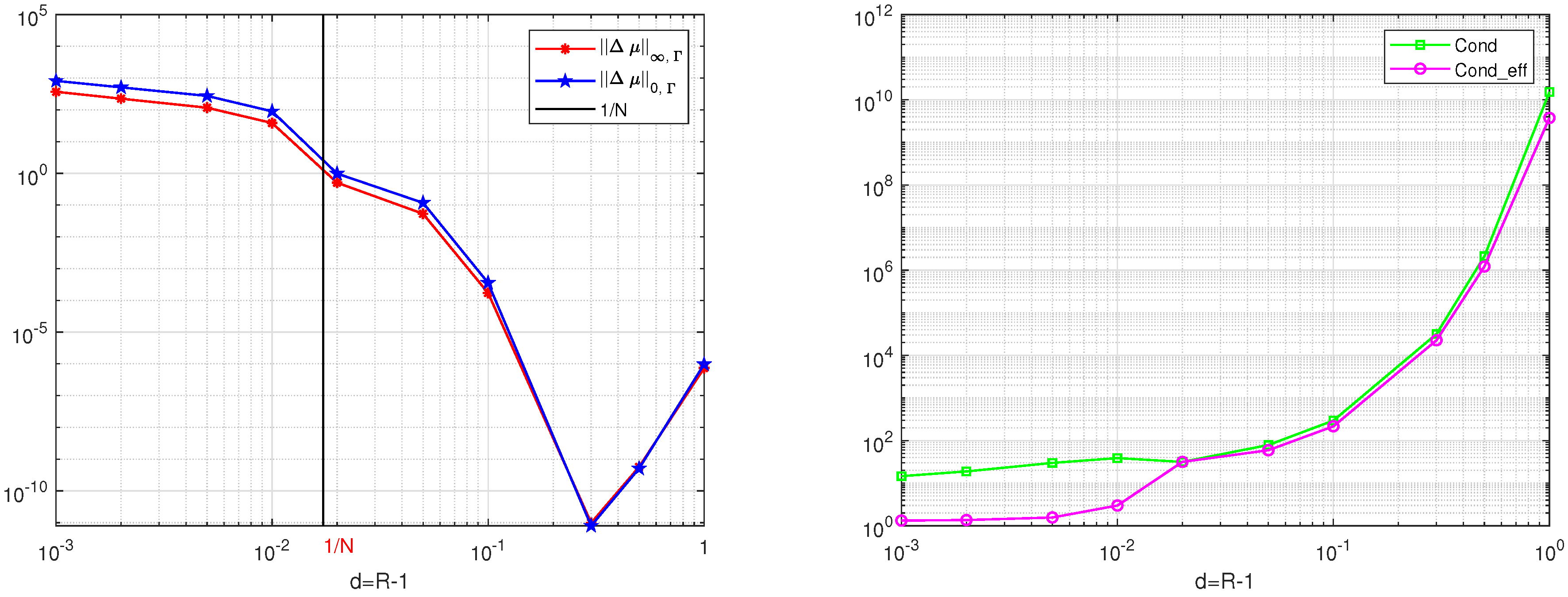
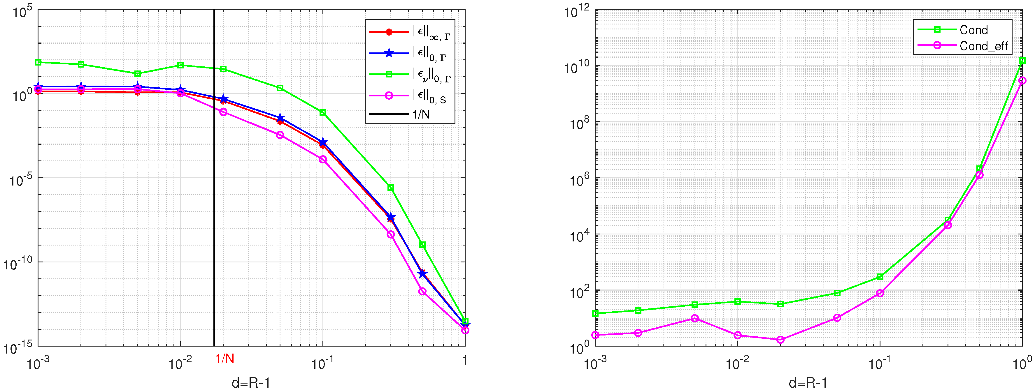
To evaluate the width of the exterior boundary layers, we choose the solution . The results are given in Table 1 and Table 2. The curves based on the results in Table 1 and Table 2 are given in Figure 1 and Figure 2. For , we have . In Table 1 and Table 2, the large errors of are given for in agreement with Proposition 3 and Corollary 2. Next, for the errors , from Proposition 3, we use , where the theoretical width . Hence, when and , we have

Table 1.
The errors and condition numbers for the DNFEM using the circular pseudo-boundaries with radius and for in the unit disk domain.
Table 2.
The errors and condition numbers for the MFS using circular pseudo-boundaries with radius and for in the unit disk domain.
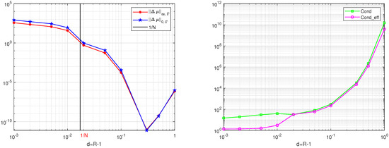
Figure 1.
The curves via R from the results in Table 1 for for the DNFEM, for , (L), and for the Cond and the Cond_eff (R).
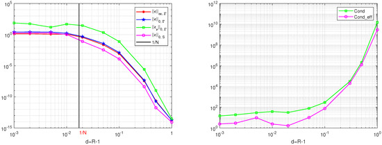
Figure 2.
The curves via R from the results in Table 2 for for the MFS, for , , and (L), and for the Cond and the Cond_eff (R).
Since on , we find from Equation (56). In Table 1, small errors of are shown for , which also supports the convergence results in Proposition 3. To achieve higher accuracy, the rule was proposed by Barnett [3]. Later, more computations were carried out for the source nodes outside the exterior boundary layers (i.e., at least at a distance larger than ).
Next, for the DNFEM, when the source nodes are as far as , the errors become larger (see Table 1 and Figure 1) due to ill-conditioning. Hence, for the DNFEM, the source nodes should be chosen not too far from (i.e., ). However, for the MFS, source nodes far from for are beneficial (see Table 2 and Figure 2). The locations of source nodes relative to in the DNFEM are more sensitive than those in the MFS.
The term “boundary layers" originated from fluid mechanics, and the thickness (i.e., width) has been studied. In this paper, we also use the “boundary layers" resulting from the singularity of the FS: as . The exterior boundary layers occur for both the DNFEM and the MFS, but the interior boundary layers occur only for the DNFEM. In [3], the width of the interior boundary layers was studied for the boundary integral equation method (BIEM). In this paper, we explore the width of the exterior boundary layers for the DNFEM and the MFS, which is consistent with [3].
3.2. Pseudo-Boundaries from Conformal Mapping
For Jordan domains, conformal mapping was employed by Katsurada and Okamoto [9] to transform both the domain boundary and the pseudo-boundary into concentric circles. Then, exponential convergence rates were obtained for analytic solutions using the MFS. We use conformal mapping for the DNFEM (as well as the MFS) to find suitable pseudo-boundaries. We can express the coordinate functions using the Fourier series, as shown in [4]:
Let and denote the uniform nodes on the unit circle with . Also, denote the boundary nodes . The conformal mapping T from the unit circle to in Equation (57) at can be defined, where the coefficients were obtained from [4]:
Let the boundary be defined by , where is a function in polar coordinates. In Equations (58) and (59), we choose and with . The pseudo-boundary of the source nodes can be determined using Equation (57) with small . For , we choose the Fourier series:
The conformal mapping T from to with , is given by Equations (60) and (61) for , where the Fourier coefficients are
and
where and with .
For disk domains S with radius a, the conformal mapping from a unit circle to a circle with radius a is given in Equations (57), (60) and (61) for , where , while all other coefficients are zero. In the general case, where is defined by , nonzero coefficients arise. The conformal mappings in Equations (57), (60) and (61) are valid only for small values of and not for large values of L.
Proposition 4.
Let denote the conformal mapping, and suppose that the -periodic function with . For Fourier expansions in Equation (57), small values of and not large values of n (i.e., not large L) are required in applications. One necessary condition is
where is a bounded constant independent of ρ and n. For the given n, the condition in Equation (66) leads to
Proof.
To find the conditions for the conformal mapping, we consider as an example. The function can be expressed using a Fourier series as follows:
where and are the true expansion coefficients. Then, we have
where the coefficients in Equation (58) are determined by
Under the assumption with , we have the bounds for the coefficients in Equations (68) and (70):
From Equation (71), we have
Since is bounded, the last term, , in the series from Equation (72) must also be bounded, which leads to the necessary condition in Equation (66). Hence, small vallues of and not large values of n are required in applications. For a given n, the condition in Equation (67) follows directly from Equation (66). This completes the proof of Proposition 4. □
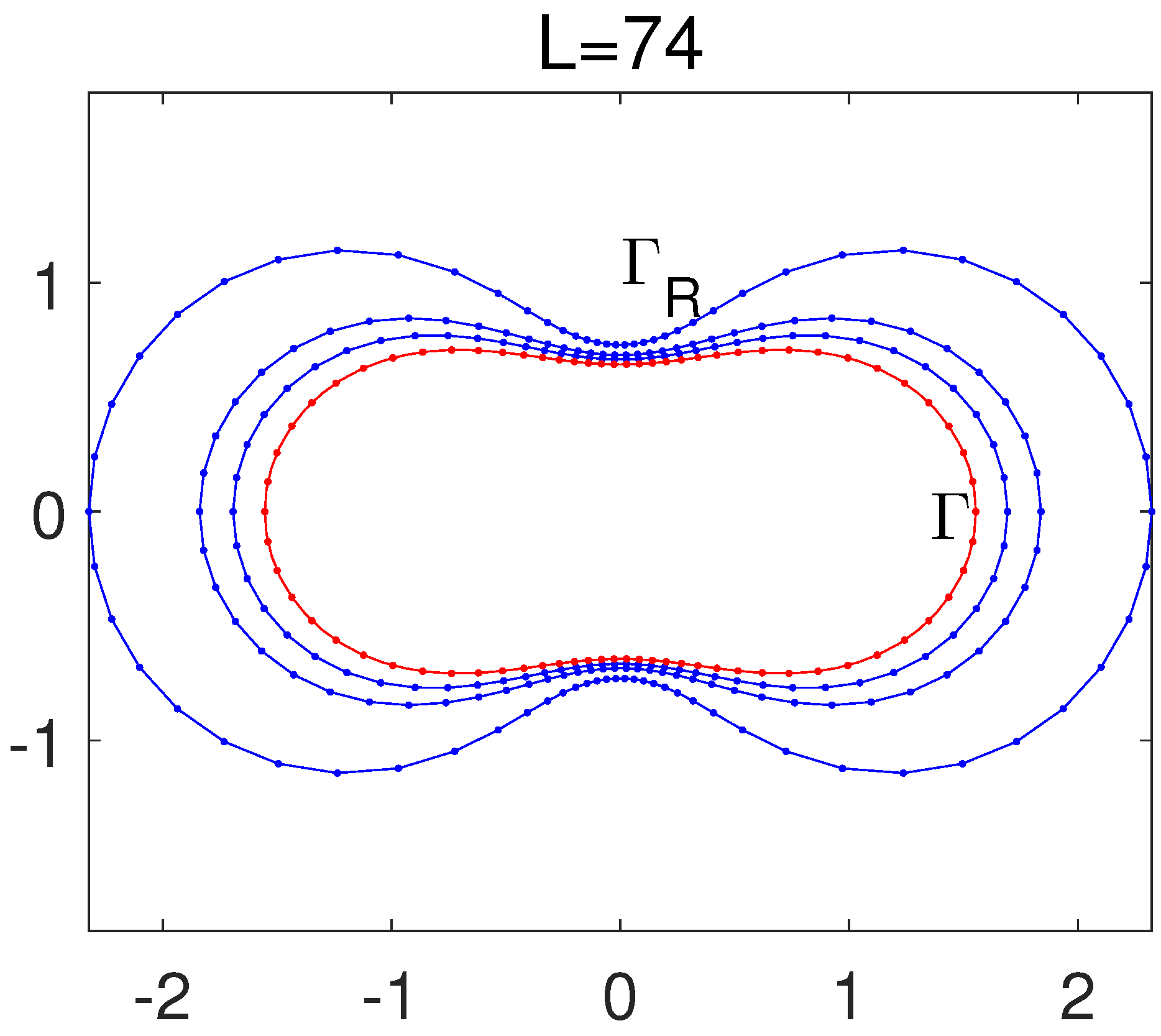
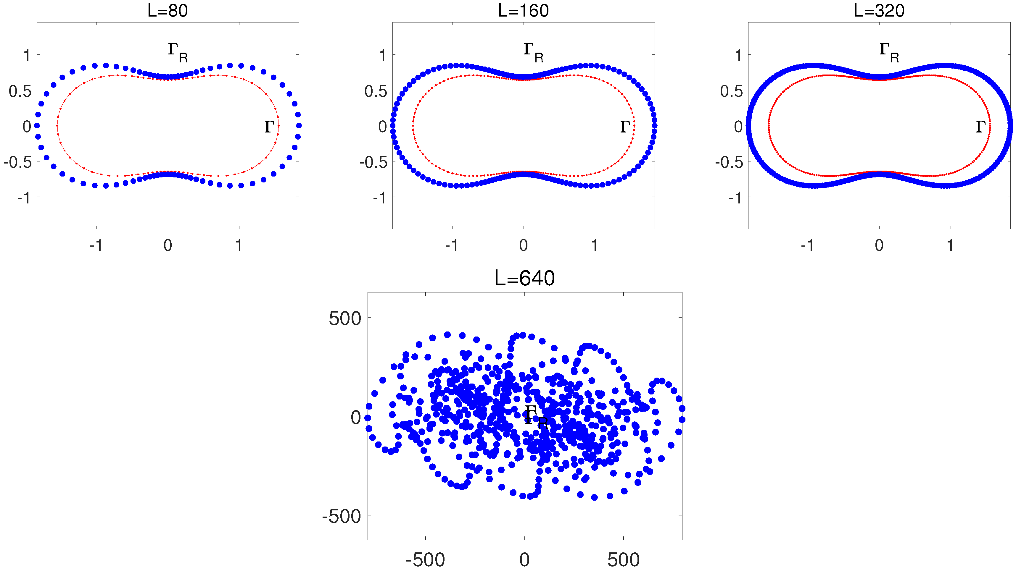
When , the Fourier expansions in Equations (60) and (61) are used. We take the peanut-like domain in Equation (85) below for testing purposes. Equations (60) and (61) work well when and , as shown in Figure 3, where only source nodes on are shown. Other source nodes can also be obtained from the same pseudo-boundary defined by Equations (60) and (61). When , the source nodes at are illustrated in Figure 4. The source nodes at are useless, and some of them at are unacceptable. Several source nodes are too close to each other at and even located inside at . Figure 4 displays a failure of the conformal mapping for . To test the failure of the conformal mapping for large , we choose the same as shown in Figure 3. In Figure 5, failure occurs for , thus verifying the necessary condition in Proposition 4.
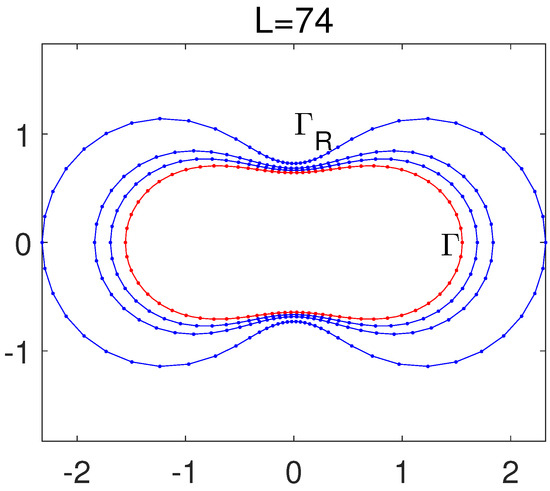
Figure 3.
The boundary of Equation (85) and the pseudo-boundaries are plotted in Cartesian coordinates, with L source nodes given by the conformal mapping when , and .
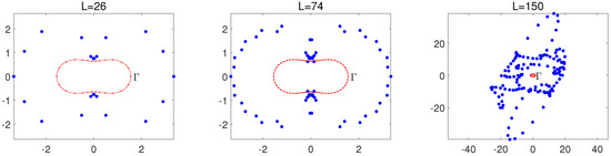
Figure 4.
The boundary of Equation (85) is plotted in Cartesian coordinates, with L source nodes given by the conformal mapping when and .

Figure 5.
The boundary of Equation (85) is plotted in Cartesian coordinates, with L source nodes given by the conformal mapping when and .
In [9], the conformal mapping was carried out using complex functions. Let , and choose the complex transformation
where the complex function with and . The complex coefficients with . Choose the complex variable . From Equation (73), we have
Then, from Equation (74), we have
where the coefficients are given by
When , the conformal mapping in Equation (75) from [9] is equivalent to Equation (57) using the Fourier series (see [14], p.178). However, for , the two algorithms are slightly different. Hence, the pseudo-boundaries from [9] are also slightly different. Under some stronger analytic assumptions for the boundary and the function f in Equation (1) (i.e., the analytic Jordan curve and the analytic function f), the distance must be small but N may be large. Then, the fast Fourier transformation (FFT) can be used for large to save CPU time. The algorithms are given in [9] (p. 128).
Remark 1.
In this paper, the number L is different from N, which is used in the DNFEM and the MFS. The L is confined to not be large (e.g., for or for for the peanut-like domain in Equation (85)), which may be smaller than N (even ) for some applications. For large N, we can use the known continuous curve in Figure 3 with and . The source nodes can be obtained directly from Equations (60) and (61) by (e.g., ) (see Section 5.2). Such algorithms are simple since the FFT in [9] can be bypassed. Hence, the small is only one key necessary condition of Proposition 4. Let us check the condition in Equation (66) again. If the boundary Γ is highly smooth with , where q is large, both ρ and n in Equation (66) could be larger. When Γ is polygons or piecewise smooth curves, we have only. The conformal mapping fails because only is allowed from Equation (66) at .
Remark 2.
In Section 3.1, the width of the exterior boundary layers is studied for disk domains with circular pseudo-boundaries. In this remark, we seek the width of the exterior boundary layers for smooth domains when the pseudo-boundaries are obtained from the conformal mapping. For the conformal mapping, the width of the exterior boundary layers can also be determined using the error estimates of the DNFEM. Consider both Γ and to be highly smooth Jordan curves. By a one-by-one conformal mapping , Γ and are, respectively, converted to a real axis and a parallel line in the complex plane (see Barnett ([3], Figure 2.1):
For the analytic solutions from the DNFEM, using the trapezoidal rule, we have the following error bounds:
When , from Equation (79). Thus, the DNFEM diverges. To achieve small , a slightly larger may be required to satisfy . This yields
The width is again found to coincide with Proposition 3 and Corollary 2 at .
The conformal mapping in Equation (77) is based on the Schwarz function in Davis [15]. In the complex plane, let and , and we have and . A closed highly smooth contour can be denoted by the analytic function , where g can be also regarded as a -periodical function in . Thus, the boundary Γ of S is denoted by with and (see [15], Chapters 2 and 5). We can relate the above mapping to the conformal mapping used here. Denote the other one-to-one conformal mapping by . From Equation (77), we have
Equation (81) also denotes circles with radii . When , we have . By the composite conformal transformation , the boundary Γ and the pseudo-boundary are converted to a unit circle and a concentric circle with radius , as shown in this section. Hence, the width, , of the exterior boundary layer is again confirmed. Hence, by using , Equation (57) is rewritten as
Remark 3.
The study in this paper can be extended to n-dimensional (nD) Laplace’s equation in Equation (1). First, consider the 3D case. Since the FS is , the Green’s representation formula in Equation (2) is modified as follows (see Atkinson [16], p.430):
where the node . The NFE from the third equation of Equation (82) is given by
For D, since the FS is given by (see Chen and Zhou [17], p.214), the NFE is given by
The algorithms of the DNFEM can be formulated similarly, where the source nodes are located outside the boundary Γ. Since the conformal mapping in Section 3.2 can be extended to nD, the techniques for locating in this paper can be developed further. Let us take the 3D case as an example. The conformal mapping in 3D is given in [8] (Section 13.2). The smooth surface Γ is converted using the conformal mapping T into a unit sphere with radius . Then, the pseudo-surface is obtained from the larger sphere with radius by applying its inverse transformation . For spheres, a distribution of good nodes is illustrated in ([8], p. 326). The collocation nodes on Γ and the source nodes on can be found using . For the conformal mapping in Section 3.2, the techniques are simple and straightforward without solving linear algebraic equations. Such a remarkable advantage remains for the conformal mapping in 3D. For the DNFEM in 3D, the stability and error analysis in Section 2 needs to explored, and the width of the boundary layers in Section 3.1 can then be discussed similarly.
4. Numerical Experiments for Non-Disk Domains
4.1. Peanut-like Domains
Denote a peanut-like domain with the boundary in polar coordinates by
We have , which yields . Denote , and . The DNFEM solution and the MFS solution can be obtained from Equations (4) and (11), respectively. Suppose that the errors and the condition have exponential rates:
Define the sensitivity index of the condition via errors by [8] (p. 345):
The index indicates the severity of the ill-conditioning. The smaller is, the better the stability and numerical performance are achieved.
4.2. Numerical Results from the DNFEM and the MFS
We choose the source function in [8] (p. 376)
where the far node is outside as . The solution is highly smooth due to being far from (see Figure 6). We choose the conformal mapping for the pseudo-boundaries, as shown in Figure 3, and list the results from the DNFEM in Table 3. In Table 3, we can see that for ,
For ,
For ,
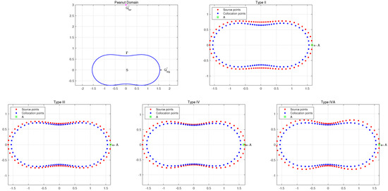
Figure 6.
The boundary with node and in Equation (88), and four pseudo-boundaries of Types II-IV and IVA with , bypassing . All boundaries are plotted in Cartesian coordinates.
Figure 6.
The boundary with node and in Equation (88), and four pseudo-boundaries of Types II-IV and IVA with , bypassing . All boundaries are plotted in Cartesian coordinates.
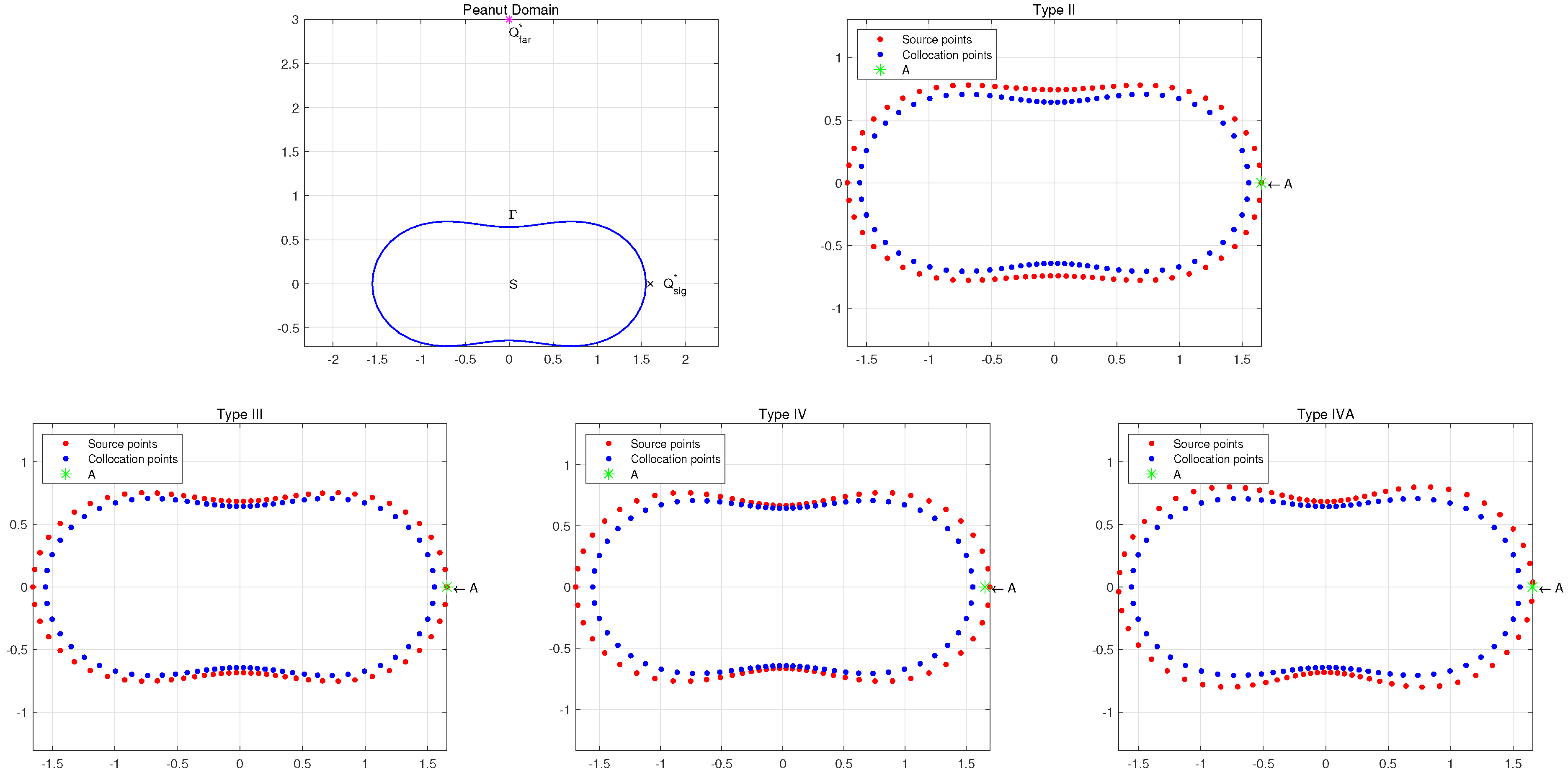
Table 3.
The errors and condition numbers for the DNFEM with using the pseudo-boundaries from Equations (60) and (61) at for the peanut-like domain, where with , and the solution given by Equation (88) with is chosen.
| N | Cond | Cond_eff | |||||
|---|---|---|---|---|---|---|---|
| 6 | |||||||
| 34 | |||||||
| 1.06 | 50 | ||||||
| 58 | |||||||
| 74 | |||||||
| 6 | |||||||
| 26 | |||||||
| 1.13 | 34 | ||||||
| 50 | |||||||
| 58 | |||||||
| 74 | |||||||
| 6 | |||||||
| 26 | |||||||
| 1.32 | 34 | ||||||
| 50 | |||||||
| 58 | |||||||
| 74 |
We can see the errors , at , respectively, and they coincide with the error estimate in Equation (40). The polynomial convergence rates of low degree are confirmed numerically, thus supporting the error analysis. Moreover, the errors , at , respectively, and they are consistent with the exponential convergence rates in Equation (79), where larger values of result in smaller errors .
For the MFS, the results are listed in Table 4. In Table 4, we can see that for ,
For ,
For ,
The DNFEM and the MFS exhibit similar numerical performance due to similar sensitivity index . The key errors in Table 3 and Table 4 for are as follows:
The DNFEM yields better accuracy for normal derivatives than the MFS. The same numerical conclusion was drawn in [4].
Let us discuss the width of the exterior boundaries in the DNFEM. For the conformal mapping, we find the width of the boundary layers as in Remark 2. Hence, for , we need We cite Equation (80) as
From Equation (104), we have at . Equation (107) leads to
Then, we require the pseudo-boundaries from the conformal mapping at . When , the numerical errors in Equation (105) are smaller, noting that . This examination supports the width study of the exterior boundary layers in Remark 2. For the pseudo-boundaries outside the exterior boundary layers, we must choose to be larger than . Note that the width of the exterior boundary layers depends on . In computations, for the given pseudo-boundaries outside , a large N will be tested to achieve small errors. If such a goal can be fulfilled, the pseudo-boundaries are already outside the exterior boundary layers.
4.3. Verification of Proposition 2 and Theorem 1
First, let us examine the norm of of the coefficients and from Table 3 and Table 4. By using and , we have the following growth rates for :
The results in Equation (109) verify that from the DNFEM in Proposition 2. Note that from Equation (110), from the MFS is even smaller. However, for singularity solutions, such as in Motz’s problem, the from the MFS is large (even huge) (see [8], Chapter 1).
Second, let us scrutinize the constants in Theorem 1. The non-uniform is given by
where . Since and , there exist the bounds
Then, we have
Hence, from Theorem 1, we have
On the other hand, we find from Table 5, that numerically,
Equation (113) coincides perfectly with Equation (112), thus verifying Theorem 1.
4.4. Computations for Solutions in the Interior Boundary Layers
The DNFEM suffers from difficulties in evaluating the solutions in the boundary layers, similar to the BEM. Note that the native algorithm in Equation (7) is ineffective for the solutions in the interior boundary layers. More efforts were made in [4] to seek simple algorithms for satisfactory solutions in the interior boundary layers. We briefly introduce them below.
Let and suppose that the solution and the derivatives from Equation (4) are known, where is the exterior normal to at . Let , and denote by the interior normal of . Also, denote the distance . From Taylor’s formula with first-order expansion at the center , we choose the interpolation solutions in the interior boundary layers from [4]:
where degree interpolations are obtained from the known solutions in Equation (4). Denote the errors of from Equation (4) by
Let , , and Equation (115) be given. For Equation (114), we have the bound from [4]:
where C is a bounded constant independent of N and .
Moreover, for high accuracy of the interpolation solutions in the interior boundary layers, we can employ the Fourier expansions, as in [4]:
where the Fourier coefficients
with , and are given from Equation (4). The interpolation in Equation (114) is modified by
Let , , and Equations (117)–(120) be given. From the solutions from the DNFEM, suppose that
For Equation (121), we have the bound (see [4])
Remark 4.
We can also replace in Equation (114) with the piecewise interpolation polynomials based on at to give the second-kind approximation
where are the piecewise q-degree interpolation polynomials. Also, we apply the Fourier series for both the solutions and their derivatives and modify Equation (121) as
The error bounds are given in [4].
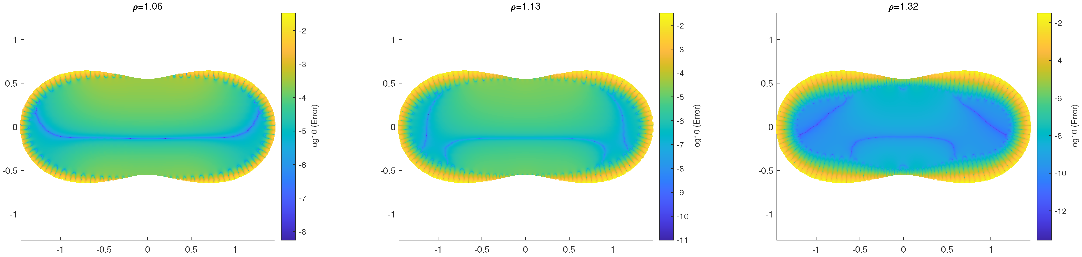
We first consider the simple algorithm in Equation (7), where the nodes Q may be located on the conformal mapping in Equations (60) and (61). We do not list the outputs in detail but provide only the errors of via Q in S in Figure 7. For the interior and exterior boundaries, the width of the interior boundaries was also given as in Remark 2. From Figure 7, the errors of the solutions in the interior boundary layers given by the native algorithms in Equation (7) are too large. On the other hand, the interpolation techniques in Section 4.4 for the computation of the interior boundary layers can be employed to give good solutions with small errors. In Figure 7, a few blue curves display higher accuracy in the numerical solutions. Unfortunately, we cannot explain the exact reasons for these outcomes (maybe due to the cancellation of rounding errors).
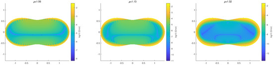
Figure 7.
The errors in S using the simple algorithm in Equation (7) are shown, with colors based on u and on from the DNFEM for , for the peanut-like domain with (L), (M), and (R). The three boundaries are plotted in Cartesian coordinates.
The normal direction is given by (see [18])
where and are the unit vectors along the X and the Y axes, respectively. For the peanut-like domain, the interior boundary is given by
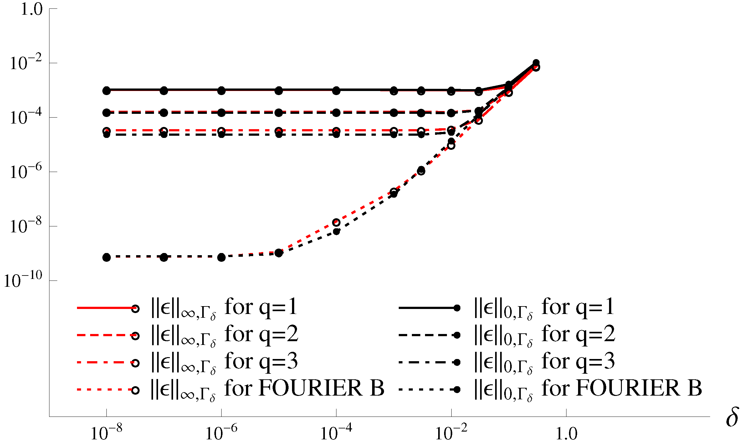
Piecewise interpolation polynomials with low degrees and Fourier series, as presented in [4], are also used to approximate by using at . The results are given in Table 6, where the second-kind approximations in Equation (123) and FOURIER B in Equation (125) from [4] are used. The error curves are shown in Figure 8, based on Table 6. When , the additional errors are dominant, as shown in [4]. Since , the Fourier series in Equation (125) yields better numerical performance. Figure 8 illustrates the importance of using Fourier series for solutions in the interior boundary layers. The numerical results of the techniques obtained with the Fourier series are consistent with the error analysis. Note that Table 6 and Figure 7 are based on Table 3 for . Hence, the width of the interior boundary layers is more important than that of the exterior boundary layers in the DNFEM.
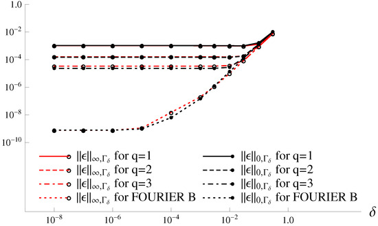
Figure 8.
The error curves based on the results in Table 6.
5. Numerical Results for Different Pseudo-Boundaries Using the DNFEM
For bounded simply connected domains, choosing optimal pseudo-boundaries is an important computational topic. We refer readers to the study of the MFS in [8]. There are two kinds of pseudo-boundaries outside of S: Case A is a closed contour, and Case B consists of two radial lines [8] (Chapter 17). In this paper, we only choose the closed contour. In this section, we re-examine the conformal mapping in Section 3.2 and employ the pseudo-boundaries with equal distances/ratios discussed in [8] (Part III). Numerical comparisons are provided for both smooth and singular solutions.
By following [8] (Chapter 15), we choose the pseudo-boundaries with equal distances/ratios to via the radial direction:
where is given in Equation (85). We consider four types of pseudo-boundaries via :
The angles may be chosen uniformly via the arc length, and the numerical results did not show better numerical performance as that for amoeba-like domains in [8] (Chapter 16), where the boundary has sharp changes of curvature. The details are omitted here. We only report the results for the DNFEM via equal angles as .
5.1. Numerical Results for Smooth Solutions
Choose the highly smooth solution in Equation (88) with . Since Type I of the circular pseudo-boundary is less efficient, we only choose Types II-IV and IVA to pass through the same node (see Figure 6). For comparison, in this paper, we restrict node to remain relatively close to the boundary because the DNFEM is more sensitive to ill-conditioning than the MFS (see Remark 5). To evaluate the numerical performance using the sensitivity index, we only evaluate the key results of the errors and Cond. The results of the DNFEM are given in Table 7. In Table 7, we can see that for Type II (equal distance) with ,
For Type III (equal ratio) with ,
For Type IV (conformal mapping) with ,
Type III (equal ratio) exhibits the best numerical performance due to the smallest sensitivity index . However, Type IVA [9] yields the smallest errors with . The key errors and conditions from Table 7 with are as follows:
Type IVA yields the smallest error ; the other three types yield similar errors . For stability, Type II yields the largest , but Type III yields the smallest .
Table 7.
The errors and condition numbers for the DNFEM using Types II-IV and IVA [9] with for the peanut-like domain, where the smooth solution in Equation (88) with is chosen.
5.2. Numerical Results for Singular Solutions
Choose the singular solution in Equation (88) with (see Figure 6). Since Type II is less effective, as seen in Section 5.1, we only use Types III, IV, and IVA passing through . For singular solutions, the pseudo-boundaries should be chosen close to (see [8], Part III). We carried out the computations with and . The results with are slightly better than those with . We only report the numerical performance with . The results are given in Table 8. In Table 8, is used for the conformal mapping. From Remark 1, we use the known continuous curve in Figure 3 with and , and the source nodes can be obtained from Equations (60) and (61) when at . For Type IVA [9], the same techniques as above are chosen for without using the FFT in [9]. In Table 8, we can see the following:
A comparison of different pseudo-boundaries is given in Table 9. Types III, IV, and IVA [9] exhibit similar numerical performance. Note that the highly smooth domain boundary is required for conformal mapping. For a polygonal or a piecewise smooth curved boundary , however, the conformal mapping fails (see Remark 1), but Types II and III work well. Types IV and IVA (conformal mappings) are rather complicated; they are beneficial for the error analysis of the analytic solutions (see Equation (79)), thus enriching the DNFEM and the MFS in wide applications.
Table 9.
Summary of the sensitivity index for the DNFEM using Types II-IV and IVA.
Table 8.
The errors and the condition numbers for the DNFEM using Types III, IV, and IVA [9] with for the peanut-like domain, where the singular solution in Equation (88) with is chosen.
Table 8.
The errors and the condition numbers for the DNFEM using Types III, IV, and IVA [9] with for the peanut-like domain, where the singular solution in Equation (88) with is chosen.
| N | Cond | Cond_eff | |||||
|---|---|---|---|---|---|---|---|
| Type III | 40 | ||||||
| Equal ratio | 80 | ||||||
| 160 | |||||||
| 320 | |||||||
| Type IV | 40 | ||||||
| Conformal | 80 | ||||||
| 160 | |||||||
| 320 | |||||||
| Type IVA | 40 | ||||||
| Conformal [9] | 80 | ||||||
| 160 | |||||||
| 320 |
Remark 5.
In Section 3.1, the DNFEM was more sensitive to ill-conditioning than the MFS. To achieve optimal convergence rates, regularization is often needed to remove severe ill-conditioning. In this paper, we do not use regularization and report numerical comparisons for the near node from Γ in this section. For far nodes and , however, regularization (such as truncated singular-value decomposition (TSVD)) is needed for the DNFEM. The details are reported elsewhere. On the other hand, good numerical solutions are given in Table 3 for three nodes , , and , where the DNFEM via the conformal mapping is chosen without regularization. The conformal mapping is more promising. The reason for this is that the ill-conditioning of the conformal mapping is similar to that in [4], where Γ and are co-circles. Good numerical solutions are given in [4] for the DNFEM without regularization.
6. Concluding Remarks
Some novelties of this paper are as follows:
- The discrete null-field equation method (DNFEM) was proposed in [4], where the discussions and computations were confined only to disk domains. It is imperative to apply the DNFEM to bounded simply connected domains, which is the goal of this paper. A stability and error analysis is performed, and better locations of source nodes are studied thoroughly (see [8], Part III).
- For bounded simply connected domains, the bounds of the condition numbers are derived and given in Theorem 1. Both the DNFEM and the MFS share similar bounds of the condition numbers. The error analysis is performed using the Galerkin approaches of the BEM in [2]. Error bounds are provided in Section 2.2, while detailed proofs are given elsewhere. The stability and error analysis provides a theoretical foundation for the DNFEM.
- In the DNFEM and the MFS, the source nodes are located not only outside S but also outside the exterior boundary layers. The width of the exterior boundary layers is derived as in Section 3.1 for the disk domains and in Remark 2 for conformal mapping. The width of the exterior boundary layers is also valid for the interior boundary layers, as shown in Section 4.4. The width study of the exterior and interior boundary layers is imperative to the DNFEM.
- For smooth boundaries of Jordan domains, the conformal mapping in [9] is proposed to find the pseudo-boundaries, where the Fourier series in [4] is applied. The algorithms are provided and the necessary conditions are given in Proposition 4. The pseudo-boundaries from the conformal mapping must be near (i.e., small ), and the number of Fourier series terms in Equation (57) is also restricted from being large.
- For peanut-like domains, the pseudo-boundaries are formulated from the conformal mapping, and numerical experiments are carried out for the DNFEM and the MFS in Section 4. The stability and error analysis in Section 2 (as well as Equation (79)) is confirmed, and the new techniques in Section 4.4 are efficient for the solutions of the DNFEM in the interior boundary layers.
- Comparisons between the conformal mapping and other pseudo-boundaries are made in Section 5, as in [8] (Chapter 16). Numerical comparisons are reported for peanut-like domains, where all pseudo-boundaries are passed through a near node to . Types IV and IVA offer similar numerical performance to Type III with equal ratios. The conformal mapping is beneficial for the error analysis of analytic solutions, and it can be extended to 3D (see Remark 3). Note that the conformal mapping fails for polygonal or piecewise curved boundaries, while Types II and III do not have such limitations.
- In summary, the algorithms of the DNFEM are much simpler than the traditional BEM. Based on the analysis, various choices of better locations of source nodes and good numerical computations, the DNFEM may become a new competent boundary method for scientific/engineering computing.
Author Contributions
Methodology & Investigation, L.-P.Z.; Writing—original draft, Z.-C.L.; Writing—review & editing, H.-T.H., M.-G.L. and A.L.K. All authors have read and agreed to the published version of the manuscript.
Funding
This work was supported by the Ministry of Science and Technology of Taiwan project 109-2923-E-216-001-MY3, and the Russian Foundation for Basic Research project number 20-51-S52003.
Data Availability Statement
I do not have any research data outside the submitted manuscript file.
Acknowledgments
We gratefully thank the reviewers for their valuable comments and suggestions.
Conflicts of Interest
The authors declare that they have no conflicts of interest.
References
- Brebbia, C.A.; Telles, J.C.F.; Wrobel, L.C. Boundary Element Techniques, Theory and Applications in Engineering; Springer: Berlin/Heidelberg, Germany; New York, NY, USA, 1984. [Google Scholar]
- Sauter, S.A.; Schwab, C. Boundary Element Methods; Springer: New York, NY, USA, 2011. [Google Scholar]
- Barnett, A.H. Evaluation of layer potentials close to the boundary for Laplace and Helmholtz problems on analytic planar domains. SIAM J. Sci. Comput. 2014, 36, A427–A451. [Google Scholar] [CrossRef]
- Zhang, L.P.; Li, Z.C.; Lee, M.G.; Huang, H.T. Discrete null field equation methods for solving Laplace’s equation; Boundary layer computation. Numer. Methods PDE 2024, 40, e23092. [Google Scholar] [CrossRef]
- Christiansen, S.; Meister, E. Condition number of matrices derived from two classes of integral equations. Math. Meth. Appl. Sci. 1981, 3, 364–392. [Google Scholar] [CrossRef]
- Doicu, A.; Mishchenko, M.I. An overview of the null-field method. I: Formulation and basic results. Phys. Open 2020, 5, 100020. [Google Scholar] [CrossRef]
- Doicu, A.; Mishchenko, M.I. An overview of the null-field method. II: Convergence and numerical stability. Phys. Open 2020, 3, 100019. [Google Scholar] [CrossRef]
- Li, Z.C.; Huang, H.T.; Wei, Y.; Zhang, L.P. The Method of Fundamental Solutions: Theory and Applications; EDP Sciences: Les Ulis, France; Science Press: Beijing, China, 2023. [Google Scholar]
- Katsurada, M.; Okamoto, H. The collocation points of the fundamental solution method for the potential problem. Comput. Math. Appl. 1996, 31, 123–137. [Google Scholar] [CrossRef]
- Dou, F.; Zhang, L.P.; Li, Z.C.; Chen, C.S. Source nodes on elliptic pseudo-boundaries in the method of fundamental solutions for Laplace’s equation; selection of pseudo-boundaries. J. Comp. Appl. Math. 2020, 377, 112861. [Google Scholar] [CrossRef]
- Li, Z.C.; Lu, T.T.; Hu, H.Y.; Cheng, A.H.-D. Trefftz and Collocation Methods; WIT Press: Southampton, UK; Billerica, MA, USA, 2008. [Google Scholar]
- Ciarlet, P.G. Basic error estimates for elliptic problems. In Handbook of Numerical Analysis; Ciarlet, P.G., Lions, J.L., Eds.; Elsevier B.V.: Amsterdam, The Netherlands, 1991; Volume II, pp. 17–351. [Google Scholar]
- Babuška, I.; Aziz, A.Z. Survey lectures on the mathematical foundations of the finite element. In The Mathematical Foundations of the Finite Element with Application to Partial Differential Equations; Aziz, A.Z., Ed.; Academic Press: New York, NY, USA, 1972; pp. 3–359. [Google Scholar]
- Atkinson, K.E. An Introduction to Numerical Analysis, 2nd ed.; John Wiley & Sons: New York, NY, USA, 1989. [Google Scholar]
- Davis, P.J. The Schwarz Function and Its Applications; The Carus Mathematical Monographs, No. 17; The Mathematical Association of America: Buffalo, NY, USA, 1974. [Google Scholar]
- Atkinson, K.E. The Numerical Solution of Integral Equations of the Second Kind; Cambridge University Press: Cambridge, UK, 1997. [Google Scholar]
- Chen, G.; Zhou, J. Boundary Element Methods; Academic Press: New York, NY, USA, 1992. [Google Scholar]
- Li, M.; Chen, C.S.; Karageorghis, A. The MFS for the solutions of harmonic boundary value problems with non-harmonic boundary conditions. Comput. Math. Appl. 2013, 66, 2400–2424. [Google Scholar] [CrossRef]

Disclaimer/Publisher’s Note: The statements, opinions and data contained in all publications are solely those of the individual author(s) and contributor(s) and not of MDPI and/or the editor(s). MDPI and/or the editor(s) disclaim responsibility for any injury to people or property resulting from any ideas, methods, instructions or products referred to in the content. |
© 2024 by the authors. Licensee MDPI, Basel, Switzerland. This article is an open access article distributed under the terms and conditions of the Creative Commons Attribution (CC BY) license (https://creativecommons.org/licenses/by/4.0/).