ADeFS: A Deep Forest Regression-Based Model to Enhance the Performance Based on LASSO and Elastic Net

Abstract

In tree-based algorithms like random forest and deep forest, due to the presence of numerous inefficient trees and forests in the model, the computational load increases and the efficiency decreases. To address this issue, in the present paper, a model called Automatic Deep Forest Shrinkage (ADeFS) is proposed based on shrinkage techniques. The purpose of this model is to reduce the number of trees, enhance the efficiency of the gcforest, and reduce computational load. The proposed model comprises four steps. The first step is multi-grained scanning, which carries out a sliding window strategy to scan the input data and extract the relations between features. The second step is cascade forest, which is structured layer-by-layer with a number of forests consisting of random forest (RF) and completely random forest (CRF) within each layer. In the third step, which is the innovation of this paper, shrinkage techniques such as LASSO and elastic net (EN) are employed to decrease the number of trees in the last layer of the previous step, thereby decreasing the computational load, and improving the gcforest performance. Among several shrinkage techniques, elastic net (EN) provides better performance. Finally, in the last step, the simple average ensemble method is employed to combine the remaining trees. The proposed model is evaluated by Monte Carlo simulation and three real datasets. Findings demonstrate the superior performance of the proposed ADeFS-EN model over both gcforest and RF, as well as the combination of RF with shrinkage techniques.

1. Introduction

One of the most critical challenges in deep learning-based models is the number of hyperparameters. Automatically reducing them can enhance the performance of DL-based models and reduce computational load. Reducing the number of hyperparameters can lead to (1) improving the performance of the model, (2) enhancing accuracy, and (3) reducing computational load. To obtain more accurate predicting performance, numerous intelligent predicting algorithms based on DL in artificial intelligence have been employed. Additionally, recently introduced hybrid models demonstrate superior performance compared to individual models [1,2,3,4,5].

Automatically reducing the number of parameters using shrinkage techniques has been shown to be effective in reducing the overfitting and computational load [6,7,8]. Parameter regularization approaches in both traditional machine learning (ML) and more recently in DL algorithms, along with tree reduction methods in tree-based algorithms, are highly effective in enhancing prediction accuracy, reducing overfitting, and decreasing computational load. This reduction typically involves removing trees that have less contribution to prediction.

Deep learning (DL) [9] is a sub-field of ML that employs deep neural networks (DNNs). DNNs have recently gained considerable popularity in different fields [10,11,12]. Although DNNs are powerful, they have many defects. The most important defect is the large number of parameters. This indicates the strong dependence of these algorithms on tuning parameters. The large number of parameters refers to overfitting and computational load challenges in which the complexity of DL models becomes high and it can cause overfitting. To control overfitting, the computational load and model’s complexity should be reduced. Sometimes, DNN models are excessively complex and require pruning to reduce their complexity and simplify their operations. In this study, forest pruning is carried out in the last layer of the cascade forest step by reducing the number of forests using shrinking methods.

Considering the above-mentioned problems, a new DL-based deep forest (DF) algorithm has recently been proposed by Zhou et al. [13] called gcforest, as an alternative to DNNs. Gcforest is an ensemble algorithm based on trees with a DF structure that incorporates the DNN and DL theory in the prediction process [14]. The DF algorithm is a combination of the ML and DL algorithms. DL part is referred to convolutional neural network (CNN) [15] which has a two-step structure. In the first stage, convolutional layers are used to extract features from raw data, while the second stage involves fully connected layers for making the final prediction. It means DF acts more like CNN [16]. In addition, DF, due to its forest and ensemble structure, works similarly to random forest (RF) [17] and leads to final prediction by ensembling the results obtained from individual trees [18].

Increasing the number of forests in the gcforest leads to a higher error rate and computational load, resulting in decreased model performance. In the present research, a hybrid DL model is proposed to enhance the performance of the gcforest algorithm. Our approach involves the use of shrinkage techniques to reduce the number of forests in the cascade forest step of the gcforest. This method focuses on improving the accuracy of the model by targeting low-performing trees, especially those with low accuracy and efficiency. The aim is to improve model performance in two ways. First, the number of gcforest forests and trees within them are reduced by eliminating low-performing forests using shrinkage techniques, as having a large number of forests can negatively impact model performance. Second, the computational load is reduced during the prediction step. The proposed model achieves significant results by removing forests and trees within them in the last layer of the cascade forest. Additionally, model performance is improved by replacing deep forest instead of RF.

This research proposes a novel approach called Automatic Deep Forest Shrinkage (ADeFS) that combines shrinkage techniques and deep forest algorithm to enhance the performance of the gcforest algorithm. Instead of using RF, the method employs deep forest as a predictor. The deep forest consists of some RFs within each layer, which increases the accuracy of gcforest compared to RF. The proposed model involves four steps. The first step, the multi-grained scanning (MGS) step, generates various feature vectors by slicing the input data under different windows. Following that, the feature vectors are inputted into the forests of this step. The produced trees in the MGS step are concatenated and enter the cascade forest (CF) step. The second step consists of multiple levels, each level containing several random forests as well as completely random forests that are extracted in the last level of cascade forests. The CRFs and RFs are used as predictors in the next step. The third one is the shrinkage step in which the produced forests in the previous step are reduced by the use of shrinkage techniques including LASSO, EN, Group Lasso (GL), and Adaptive Lasso (AL). These reducers remove the trees from the model, decrease computational load, and finally improve gcforest performance. The final step is the ensemble step in which the remaining forests from the previous step are aggregated by the simple average ensemble method. The contribution of this paper can be summarized in the following main aspects:

➢

By integrating DL algorithms with shrinkage techniques, we have devised a model aimed at reducing the number of trees within the DF. This reduction not only decreases the computational load during the prediction phase but also boosts the overall performance of the model.

➢

To the best of our knowledge, no prior research has been performed on the combination of statistical methods with the DF algorithm to enhance the performance of the gcforest algorithm.

➢

To enhance the performance of gcforest, shrinkage techniques are employed to select appropriate trees and remove some trees to reduce their number.

➢

Given the tendency of random forest to overfit, in this paper, RF is replaced with DF.

The rest of this paper is organized as follows: Section 2 includes a review of previous research, primarily focusing on the research status and existing problems associated with deep forests. In Section 3, an overview of the gcforest algorithm is provided, along with the compression techniques utilized in this study. Section 4 outlines the architecture and summarizes the proposed approach. The outcomes of the simulation study and the evaluation of the proposed model are presented in Section 5. Finally, a summary of the results and conclusions is presented in Section 6.

2. Related Works

This section presents a summary of the literature on DL-based deep forests, with a focus on ML and DL models that use statistical methods to reduce overfitting and computational load. The reviewed papers highlight prediction models based on RF and CNN. Furthermore, recent DF models are discussed, particularly those related to the early detection of COVID-19, drug combination prediction, and strategies for overcoming overfitting.

Each part of the RF and CNN algorithms has its own deficiencies, leading to the proposed gcforest. One of these deficiencies is overfitting, which occurs when the size of training data is relatively small and the number of trees in RF is relatively large. Even when the correlation between RF trees is high, it can still lead to overfitting. To address this problem in the RF algorithm, Farhadi. Z et al. [7] presented the RARTEN framework. This framework combines shrinkage techniques with RF to decrease the number of trees. It achieves this by selecting efficient trees using shrinkage techniques like Lasso and elastic net. Through this approach, the RARTEN framework enhances the original RF model by controlling overfitting and reducing computational load. In addition, in another study, the authors introduced ECAPRAF [6], considered a hybrid model that leveraged k-means clustering to homogenize input data and reduce the number of trees within clusters. Similarly to the previous model, ECAPRAF achieved notable results compared to the original RF. In these papers, to select the RF trees in order to reduce the number of them, the feature selection property of shrinkage techniques is used.

In certain scenarios, the extensive utilization of learners in ensemble learning can significantly increase both computational load and overfitting, creating challenges to model performance. Ensembling emerges as a powerful technique to effectively address these issues. Farhadi et al. [8] recently introduced the Ensemble of Reduced Deep Regression (ERDeR) model as a novel approach This model leverages deep regressions, shrinkage techniques, and ensemble approaches as learners, aggregators, and reducers, respectively. This innovative combination aims to enhance the model’s performance by leveraging shrinkage techniques such as LASSO and EN to effectively decrease the number of learners. In [19], other types of feature selection methods were employed as a combinatorial optimization problem, which improved the performance of the Forest Optimization Algorithm [20] by removing irrelevant and redundant features. In the present paper, through combining gcforest with shrinkage techniques, the performance of the gcforest is enhanced by removing ineffective forests and trees inside of the forests using LASSO and elastic net.

The DF algorithm is utilized in various fields, including drug combination [21,22,23], the chemical industry [24,25], disease diagnosis [26,27,28], image processing [29,30,31], etc. One instance is its use in age estimation from facial images through the gcforest algorithm in [32]. Another example is the application of the cascade DF algorithm in the classification of cancer types based on gene expression data in [33]. The researchers made improvements to the gcforest algorithm and proposed a new algorithm called BCDForest. It incorporated a multi-class and diversity-based scanning strategy to promote diversity in the collection. The strategy involved using different training data and enhancing important features at each layer of the cascade forest. In [34], the AFS-DF algorithm was introduced, which aimed to classify individuals with COVID-19 based on their chest CT images. The method extracted the location’s specific features. A DF model was then utilized to learn high-level representations of characteristics.

In recent years, there have been many improvements in the algorithms of deep forests. In 2022, Zhang Wei et al. [35] published the paper “EC-DFR: an enhanced cascade-based deep forest model for drug combination prediction”, wherein the authors proposed an improved deep forest regression algorithm for drug combination. In 2021, Heng Xia et al. [36] published a paper introducing an improved algorithm for DF regression with the structural model without changing. RF, CRF [37], GBDT, and XGBoost were used as sub-forests at each layer to enhance the variety. There are also numerous studies showing the performance of deep forest algorithms [38,39,40]. A summary of studies using DF in the literature is given in Table 1.

Table 1. Summary of related work on various DL-based approaches for deep forest.

Ref.	Approach	Objective	Challenges of the Approach
[27]	DL-based DF model	A transfer learning method and a deep forest-based model are employed for detecting COVID-19 infection from chest X-ray (CXR) images.	X-ray image features are extracted using a widely recognized deep transfer learning model, which offers the advantage of requiring fewer parameter settings compared to deep CNNs. Following feature extraction, a DF model is employed to predict COVID-19 infection in patients. This DF model, based on ensemble learning, is known for its minimal requirement for hyperparameter tuning.
[41]	Deep forest	Design an intelligent CTG classification model based on Deep Forest for antepartum fetal monitoring.	To address the challenge of distinguishing between normal and suspicious classes in antepartum cardiotocography (CTG) classification, this study employed principal component analysis (PCA) and visualization techniques to analyze the distribution characteristics of CTG data. Following data preprocessing, a DF multi-granularity scanning approach was utilized to explore the interconnections among different characteristics. Subsequently, the CF phase was implemented, integrating various classifiers such as RF, Weighted Random Forest (WRF), CRF, and Gradient Boosting Decision Tree (GBDT), to perform deep iterations and achieve the optimal model performance.
[42]	Deep forest ensemble learning	A novel computational method, called DFELMDA, was proposed for predicting miRNAs associated with diseases. This method utilized a set of DF-based models built on autoencoders for feature learning.	A novel feature representation strategy is presented in this study, designed to obtain diverse features for each miRNA-disease relationship. Two types of low-dimensional feature representations are extracted using two deep autoencoders in this approach. These representations are then utilized to predict miRNA-disease associations. The final prediction scores are generated using a deep random forest, and these scores are combined to produce the ultimate prediction results. The performance comparison of the proposed method, DFELMDA, with several classical methods is conducted by the use of the Human microRNA Disease Database (HMDD) dataset.
[43]	Composition of deep forest and Bayesian optimization	Developing the deep forest model for rockburst prediction	To address the challenges of overfitting and hyperparameter tuning in selecting a base classifier for predicting rockburst, this study uses the combination of Bayesian optimization (BO) and DF. BO is utilized to fine-tune the hyperparameters of a deep forest model, which shows to be effective in rockburst prediction. By constructing a probabilistic model of the objective function, BO intelligently selects the hyperparameter configuration to determine the next point, thereby enhancing the deep forest model’s performance in predicting rockburst events.
[44]	Combination of deep forest and EN to predict protein–protein interactions	The objective of this model was to accurately predict protein–protein interactions (PPIs) using advanced feature extraction and a deep forest ensemble learning approach to improve prediction accuracy and reliability.	A novel method for predicting protein–protein interactions (PPIs) using a deep-forest-based approach was introduced. Key features were extracted using PAAC, Auto, MMI, CTD, AAC-PSSM, and DPC-PSSM. These features were then optimized with elastic net to improve prediction accuracy. The XGBoost, random forest, and extremely randomized trees were ensembled to construct the GcForest-PPI model.
[45]	Active preference-based deep forest	The objective of this model is to enhance survival prediction accuracy by integrating doctors’ empirical knowledge using deep forest and active preference learning.	A survival prediction expert system was developed, integrating deep forest and active preference learning to incorporate doctors’ empirical knowledge. Firstly, feature dimensionality was reduced with doctor input for clinical relevance. Secondly, estimators were trained to simulate clinical predictions, and doctors provided preferences based on their experience. Finally, a recursive radial basis function learned these preferences and assigned weights to the estimators.

3. Materials and Methods

3.1. Deep Forest Regression

The deep forest algorithm, also known as gcforest [13], follows a structure similar to deep learning and employs an ensemble learning technique involving decision trees. Like DNNs, this algorithm leverages representation learning and has a layered structure in which each layer consists of multiple forests. This model is composed of two main components: the first part is multi-grained scanning, in which the raw features are segmented via a sliding window technique with varying window sizes, obtaining feature vectors. Finally, these vectors are employed to train both CRF and RF. Each forest includes several decision trees and their results are concatenated together and fed into the next step. The second part consists of a cascade structure with different levels, called cascade forest. Each level receives the information and features processed by the preceding. The number of levels is automatically determined based on the raw input data. The forests within each level can be any tree-based method, such as RF, CRF, XGboost [46], etc. The number of forests per layer and the number of trees in each forest are hyperparameters. In the last layer, the output of the forests is the average of the produced trees, which are ensembled together to obtain the final prediction.

In DF, within each layer, RFs are substituted by neurons in original DNNs, allowing the algorithm to perform representation learning. In other words, like RF, the structure of this algorithm is based on decision trees, which are ensembled eventually. Using decision trees in gcforest allows the algorithm to handle non-linear relationships between inputs. Furthermore, leveraging RFs in the cascade forest step allows the algorithm to easily handle high-dimensional input data. In general, the gcforest algorithm provides an alternative approach to traditional DNNs which are more efficient in handling specific types of data. Nonetheless, like any ML algorithm, gcforest has specific pros and cons and may not be the best choice for every type of data or task.

3.2. Shrinkage Techniques

Shrinkage techniques are a group of techniques that can perform feature selection, tree selection [6,7], and penalization model [47,48] as a part of the model-building process. These methods, as a part of statistical methods, are widely employed in machine learning. The most common shrinkage techniques include LASSO, EN, AL, and GL. In the following, each of these methods will be briefly reviewed, and their strengths and weaknesses will be examined. To enhance the accuracy of the gcforest algorithm and reduce computational load during prediction, the deep forest algorithm is combined with shrinkage techniques. Clearly, selecting an appropriate shrinkage technique for tree selection is crucial in improving the algorithm’s performance. Therefore, we propose combining statistical and artificial intelligence methods to enhance the efficacy of the DF.

LASSO: Lasso regression technique, introduced by Tibshirani in 1996 [49], is a popular technique for variable selection. It is particularly useful in situations with a high number of predictors or when collinearity exists among them. This technique aims to minimize both the Residual Sum of Squares (RSS) and prediction error. It achieves this by applying an ${\mathcal{l}}_1$-norm penalty on the absolute sum of the regression coefficients, resulting in an automatic reduction in certain coefficients to zero during the variable selection process. The remaining variables with non-zero coefficients are then used in the final prediction. However, similar to any other technique, it has specific advantages and disadvantages. One of the disadvantages is that the maximum number of selected variables is limited by the number of samples, and another is its inability to select variables as a group [50].

In LASSO estimation, the ${\mathcal{l}}_1$-norm is applied as part of the penalized least squares, defined as follows:

$${\widehat{\beta }}^{lasso}=\begin{array}{c}argmin\\ \beta ϵ{\mathbb{R}}^p\end{array}\left\{{\displaystyle \frac{1}{2}}{‖Y-X\beta ‖}_2^2+{\lambda ‖\beta ‖}_1\right\}$$

(1)

where ${‖\beta ‖}_1$ and $\lambda \ge 0$ are penalty functions under ${\mathcal{l}}_1$-norm and tuning parameters to control the shrinkage rate, respectively.

Elastic Net: Elastic net regression is a variable selection technique used to overcome some of the limitations of ridge and lasso methods. The technique was first introduced by Zou and Hastie [51] in 2005 and has since become a popular approach in the analysis of high-dimensional data. It combines the advantages of both ridge and lasso techniques by employing a linear combination of ${\mathcal{l}}_2$- and ${\mathcal{l}}_1$-norm penalties to minimize the loss function. Automatic variable selection and continuous shrinkage are provided by EN with the ability of selecting groups of correlated variables. The main objective is to minimize coefficients and estimate a model based on non-zero coefficients.

The EN penalty is formed by combining two penalties, namely ${\mathcal{l}}_2$- and ${\mathcal{l}}_1$-norm, which objective function can be defined as follows:

$${\widehat{\beta }}^{elastic}=\begin{array}{c}argmin\\ \beta \end{array}\left\{{\displaystyle \frac{1}{2}}{‖y-X\beta ‖}^2+\lambda \left[{\displaystyle \frac{1}{2}}\left(1-\alpha \right){‖\beta ‖}_2^2+\alpha {‖\beta ‖}_1\right]\right\}$$

(2)

where ${‖\beta ‖}_1=\sum _{j=1}^p\left|{\beta }_j\right|$ and ${‖\beta ‖}_2^2=\sum _{j=1}^p{\beta }_j^2$ are ${\mathcal{l}}_1$-norm and ${\mathcal{l}}_2$-norm, respectively. α and $\lambda \ge 0$ are a hyper parameter and tuning parameter that determine the balance between the ${\mathcal{l}}_1$ and ${\mathcal{l}}_2$ penalties. For α = 1, the EN penalty is equivalent to the ${\mathcal{l}}_1$ penalty [49] (Lasso), and for α = 0, it is equivalent to the ${\mathcal{l}}_2$ penalty [52] (ridge).

Adaptive Lasso: Adaptive Lasso [53] is a modified form of the Lasso method with its own advantages, capable of reducing some coefficients to zero. This technique performs variable selection and shrinkage by weighting the penalty function. The weight vector is defined as $\widehat{w}={\displaystyle \frac{1}{{\left|{\widehat{\beta }}_{ols}\right|}^{\gamma }}}$, where ${\widehat{\beta }}_{ols}$ is the ordinary least squares (OLS) estimate of the i-th regression coefficient. The tuning parameter $\gamma$ controls the degree of shrinkage. One advantage of AL is its ability to perform variable selection even in cases where the number of predictors is substantially larger than the sample size. This is because the AL can reduce some coefficients to zero exactly, effectively removing the corresponding predictors from the model. If the number of predictors (p) is greater than observations (n), ($p>n$), the ridge estimator ${\widehat{\beta }}_{ridge}$ can be used instead of the ordinary least squares estimator $\widehat{\beta }\left(ols\right)$.

The AL estimator is defined as follows:

$${\widehat{\beta }}^{Alasso}=\begin{array}{c}argmin\\ \beta \end{array}\left\{{‖y-X\beta ‖}^2+\lambda \sum _{j=1}^p{w}_j\left|{\beta }_j\right|\right\}$$

(3)

where y is the response variable, X is the design matrix of predictors, $\beta$ is the vector of coefficients, parameter $\lambda$ controls the overall strength of the penalty, and $w_j$ is the weight assigned to the j-th coefficient in the penalty term.

Group Lasso: The Group Lasso estimator, proposed by Yuan and Li [54] in 2006, is a shrinkage technique that extends the Lasso method to perform variable selection at the group level. It is used to select groups of related variables in high-dimensional data as well as to identify groups of variables. In our proposed model, Group Lasso selects trees as a group and applies shrinkage to them. This means that all the coefficients within a group become either zero or non-zero together. The trees with non-zero coefficients remain in the model as a group, while the rest of the predictor variables are removed. To achieve this grouping, the parameter vector β is divided into groups ${\mathcal{G}}_1,{\mathcal{G}}_2,\dots ,{\mathcal{G}}_q$ where $\bigcup _{j=1}^q{\mathcal{G}}_j=\left\{\mathrm{1,2},\dots ,p\right\}$. The vector β is then modified based on this grouping.

$$\beta =\left({\beta }_{{\mathcal{G}}_1},{\beta }_{{\mathcal{G}}_2},\dots ,{\beta }_{{\mathcal{G}}_q}\right),{\beta }_{{\mathcal{G}}_j}=\left\{{\beta }_r;r\in {\mathcal{G}}_j\right\}$$

The Group Lasso penalty is formulated as follows:

$${\widehat{\beta }}^{glasso}=\begin{array}{c}argmin\\ \beta \end{array}\left\{{{\displaystyle \frac{1}{2}}‖y-{\beta }^{T}X‖}^2+\lambda \sum _{j=1}^q{m}_j\left|{\beta }_{{\mathcal{G}}_j}\right|\right\}$$

(4)

where $m_j$ balances between groups of different sizes. This is because if the groups have different numbers of variables, then the penalty term would have a stronger effect on the groups with fewer variables. To address this issue, the coefficient $m_j$ is defined as follows:

$$m_j=\sqrt{T_j}$$

where $T_j$ indicates the number of variables in the j-th group.

4. Structure of the Proposed Model

To enhance the DF accuracy and reduce computational load, a novel approach is proposed that combines the gcforest algorithm with shrinkage techniques, as depicted in Figure 1. This model comprises four key steps. Firstly, the sliding window method, known as MGS, is employed to capture the relationships among raw input features. The second step, known as cascade forest (CF), is structured by its level-by-level structure. The number of levels and complexity of this step are determined based on the input dataset. Within each CF level, low-level and high-level features are combined. RF and CRF are embedded in each level, each consisting of several DTs. Some of these trees may perform well and have high accuracy and precise output, while others may not. Therefore, a shrinkage step is added to the model to remove the poorly performing forests. The third step, known as the shrinkage step, involves techniques such as LASSO, EN, GL, and AL, which reduce the number of trees in the last level of the CF. These techniques automatically keep the forests that perform well in the model and remove the others with poor performance. Finally, in the last step, the remaining forests from the previous step are aggregated using an ensemble method for the final prediction.

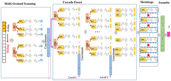
Figure 1. Overall architecture of our proposed model (ADeFS).

First step (Multi-Grained Scanning): MGS step is a crucial component of the gcforest algorithm, constructed to extract significant features from the input data. It employs a sliding window approach with various window sizes to scan the raw input features, generating a feature vector for each window. These feature vectors are then used to create RF and CRF. CRF is similar to RF, with the only difference being that it selects only one feature from all the available features, while RF selects $\sqrt{p}$ features (where p is the number of input features). Each forest comprises multiple trees, and the performance of these forests varies based on the number of trees. Following the sliding operation, the generated feature vectors are fed by the forests. Finally, the outputs of forests are concatenated at this step. Figure 2 illustrates the architecture of the MGS step.

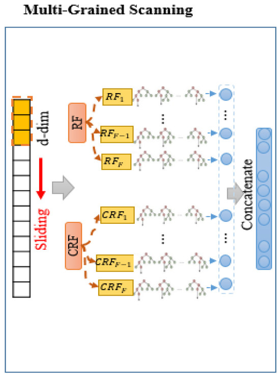
Figure 2. Architecture of the multi-grained scanning (MGS) step in the proposed model.

Second step (Cascade Forest): In the cascade forest (CF) step, a hierarchical structure is employed, where each level integrates information from the previous level with new features. At each level, two types of forests are used: RF and CRF, each consisting of F forests and M trees. The value of F is a hyperparameter that can be determined based on the specific context. DTs form the basis of CF’s operations. To make a prediction within each forest, the average of the leaf node values in the decision tree is computed. The output of each forest at each level is a prediction vector, which is then concatenated with the original input and utilized as input for the next level. The architecture of the CF step is depicted in Figure 3.

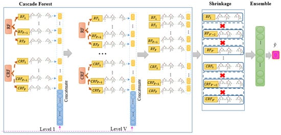
Figure 3. Architecture of the cascade forest (CF) step in the proposed model.

Let $\left\{\left({\mathit{x}}_1,y_1\right),\dots ,\left({\mathit{x}}_N,y_N\right)\right\}$ be a dataset that is divided into a training set $D=\left\{\left({\mathit{x}}_1,y_1\right),\dots ,\left({\mathit{x}}_k,y_k\right)\right\}$ and a test set $Z=\left\{\left({\mathit{x}}_{\mathrm{k}+1},y_{\mathrm{k}+1}\right),\dots ,\left({\mathit{x}}_N,y_N\right)\right\}$. The forests, each consisting of M trees, are trained. The trees within each forest are expressed as follows:

$$T^f=\left[{\mathrm{T}}_1^f,{\mathrm{T}}_2^f,\dots ,{\mathrm{T}}_{M_f}^f\right];\hspace{1em}\hspace{1em}\hspace{1em}f=\mathrm{1,2},\dots ,F$$

(5)

The obtained prediction for the f-th forest is equal to the following:

$$P^f\left(\mathit{x}\right)={\displaystyle \frac{1}{M_f}}\sum _{m=1}^{M_f}O\left({\mathrm{T}}_m^f,\mathit{x}\right)$$

(6)

where $M_f$ represents the number of DTs in the f-th forest.

For all the forests in the v-th cascade level, the distribution of predicted values is obtained as follows:

$$P_v\left(\mathit{x}\right)=\left\{{\mathrm{P}}_v^1\left(\mathit{x}\right),{\mathrm{P}}_v^2\left(\mathit{x}\right),\dots ,{\mathrm{P}}_v^{F^{*}}\left(\mathit{x}\right)\right\}$$

(7)

The final prediction for sample Z is equal to the following:

$$\widehat{y}\left(\mathit{x}\right)=avg\left({\mathrm{P}}_v\left(\mathit{x}\right)\right)$$

(8)

Third step (Shrinkage): In tree-based algorithms, the excessive number of trees can lead to issues like overfitting, high computational load, increasing error rates, and decreasing algorithmic performance. Since the gcforest algorithm employs RF, a type of tree-based approach, for data training at different levels, having too many trees can negatively impact the model’s performance. To counteract this issue, shrinkage techniques such as LASSO, EN, GL, and AL are employed to reduce the number of trees in the last level of the gcforest algorithm. This reduction is aimed at retaining the most influential trees while enhancing the model by removing the less effective ones. Finally, the number of forests in the last CF layer will be decreased from $\left\{{\mathrm{P}}_v^1\left(\mathit{x}\right),{\mathrm{P}}_v^2\left(\mathit{x}\right),\dots ,{\mathrm{P}}_v^F\left(\mathit{x}\right)\right\}$ to $\left\{{\mathrm{P}}_v^1\left(\mathit{x}\right),{\mathrm{P}}_v^2\left(\mathit{x}\right),\dots ,{\mathrm{P}}_v^{F^{*}}\left(\mathit{x}\right)\right\}$, where $F^{*}<F$ and $F^{*}$ shows the remaining forests after shrinkage. The structure of the shrinkage step is depicted in Figure 4.

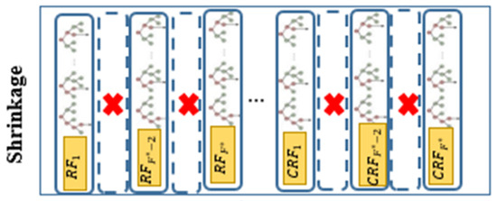
Figure 4. Architecture of shrinkage step in the proposed model.

Fourth step (Ensembling): The gcforest algorithm is designed as an ensemble method, utilizing forests as learners at different levels of the CF. The learners encompass a range of tree-based algorithms, such as RF, CRF, and XGBoost. In the present work, RF and CRF are specifically utilized. Various ensemble methods exist, with the simple average method chosen for this research. In our approach, shrinkage techniques are employed to prune trees in the former step. Afterward, the remaining forests are aggregated using the simple average method.

5. Experimental Results

In this section, our experimental research is conducted on three real datasets and one Monte Carlo simulation dataset. These datasets include the Boston housing price, real estate valuation, and Gold price per ounce. The performance evaluation of our proposed model is based on these datasets. Further details regarding these datasets are presented in Table 2.

Table 2. Details of datasets used for experimental evaluation.

Dataset	No. of Observations	No. of Features	No. of Training Samples	No. of Test Samples
Boston Housing Prices	506	13	407	99
Real Estate Valuation	414	5	332	82
Gold Price per Ounce	698	80	558	140
Simulation Data	500	7	400	100

5.1. Simulation Study Design

In the present study, a combination of DL-based algorithms and statistical techniques is proposed to reduce the number of forests in the cascade forest step. This is aimed at enhancing the performance of the gcforest algorithm while reducing computational load. The proposed model consists of four steps: (1) multi-grained scanning to extract the relationship between input features, (2) cascade forest to generate forests as predictors, (3) shrinkage techniques as a reducer to decrease the number of forests and improve the performance of the model, and (4) ensembling to aggregate the remaining forests in the model. To evaluate the performance of this method, three criteria MSE, RMSE, and MAE are used, as shown in Equations (10)–(12).

In this study, a simulation dataset is examined, comprising n = 500 random samples and p = 7 independent variables, as shown in Table 3. The original dataset is assumed to be generated from a standard normal distribution $N\left(\mathrm{0,1}\right)$ for the variables $x_1,x_2,x_3,x_4,x_5,x_6,x_7$. The corresponding linear regression model for these variables is presented as follows:

$$\begin{array}{c}y={\beta }_0+{\beta }_1{\mathrm{x}}_1+{\beta }_2{\mathrm{x}}_2+{\beta }_3{\mathrm{x}}_3+{\beta }_4{\mathrm{x}}_4+{\beta }_5{\mathrm{x}}_5+{\beta }_6{\mathrm{x}}_6+{\beta }_7{\mathrm{x}}_7+\epsilon \\ y=3-5.5{\mathrm{x}}_1+7.3{\mathrm{x}}_2+9{\mathrm{x}}_3+10.3{\mathrm{x}}_4-7{\mathrm{x}}_5+1.5{\mathrm{x}}_6+0.9{\mathrm{x}}_7\end{array}$$

(9)

where $\epsilon$ follows a normal distribution $N(0,{\mathsf{\sigma }}^2)$, where ${\mathsf{\sigma }}^2$ is equal to ${\displaystyle \frac{1}{3}}$ of the standard deviation of $y_1$.

Table 3. Hyperparameters and settings for the experimental evaluation of the proposed model (AdeFS).

Hyper-Parameters	Description	Setting
Sample size	Total number of observations	n = 500
Features	No. of independent variables for the linear model	p = 7
No. of DT in MGS step	No. of decision trees in the multi-grained scanning step	30, 100, 200
No. of total cascade forest	No. of forests in the cascade level	200, 300, 500
No. of random forest	No. of RFs in cascade level	100, 150, 250
No. of cascade trees	No. of DTs in the RF and CRF	101
Iteration	No. of repetitions of simulation	100

The simulation dataset is partitioned into training and test sets, comprising 80% and 20% of the data, respectively. To train the model, the relationships between the raw input features are extracted in the MGS step using a sliding window with a size of six. Each slide generates a feature vector that is fed by four forests, consisting of two RFs and two CRFs. The 30, 100, and 200 DT are employed in these forests. The obtained predictions from these trees are then concatenated to form the input for the next step.

The CF step comprises various levels and forests, with the number of layers and model complexity determined based on the dataset. Each level includes two types of forests, namely RF and CRF with 100, 150, and 250 forests for each type. In total, there are 200, 300, and 500 forests in this step. The number of forests is a hyperparameter that can influence the model’s performance. In each forest, 101 decision trees are embedded, which is a constant value in all considered states. The outputs of forests at each cascade level are concatenated, and after merging with the main input vector, they are fed into the next cascade level. This process continues until the final output of the last level is obtained.

The shrinkage step, which is the main and innovative aspect of this paper, employs Lasso, EN, GL, and AL techniques to reduce the number of forests and trees within them in the last layer of the CF. This reduction is aimed at improving the model’s performance while decreasing the computational load. Notably, the forests are automatically selected without prior choice at the last level. Subsequently, a subset of these forests and trees is removed to estimate a new model based on the remaining forests. The final prediction results from aggregating the remaining forests using the SA method.

Simulation Results

In evaluating the proposed model, evaluation criteria such as Mean Squared Error (MSE), Root Mean Squared Error (RMSE), and Mean Absolute Error (MAE) are employed, as described in Equations (10)–(12). The results are obtained through 100 iterations. The gcforest algorithm is implemented using the scikit-learn package in Python 3.9.16 environment. Moreover, the glmnet and gglasso packages are accomplished to execute the shrinkage step in the R environment (R 4.2.2).

$$MSE={\displaystyle \frac{\sum _{i=1}^N{\left(y_i-{\widehat{y}}_i\right)}^2}{N}}$$

(10)

$$RMSE=\sqrt{{\displaystyle \frac{\sum _{i=1}^N{\left(y_i-{\widehat{y}}_i\right)}^2}{N}}}$$

(11)

$$MAE={\displaystyle \frac{\sum _{i=1}^N\left|y_i-{\widehat{y}}_i\right|}{N}}$$

(12)

where ${\widehat{y}}_i$ is the predicted value, $y_i$ is the true value of the $i$-th sample, and N is the sample size.

Table 4 presents a comparative analysis of the obtained results from the five proposed models on the simulation dataset. The findings indicate that the gcforest model shows poor performance compared to the ADeFS-EN, ADeFS-Lasso, and ADeFS-GL models. This is primarily due to the high computational load caused by the presence of an extensive number of trees. Additionally, the ADeFS-AL model demonstrates poor performance compared to the other proposed hybrid models. This is because unlike ADeFS-EN, ADeFS-AL cannot do the shrinkage and selection of the forests as a group.

Table 4. Comparison of the ADeFS model under different combinations with other models on the simulation dataset.

		Models	MSE	RMSE	MAE
Mgstree = 30	Nforest = 200	Deep forest	58.4175072	7.643134645	5.668985288
		ADeFS-Lasso	58.4342965	7.618246664	5.854352756
		ADeFS-EN	58.32221661	7.611073122	5.850385868
		ADeFS-GL	58.41499258	7.617109686	5.853935636
		ADeFS-AL	58.58886025	7.628993075	5.860551531
	Nforest = 300	Deep forest	58.42288448	7.617751383	5.853055381
		ADeFS-Lasso	58.44991175	7.619516167	5.854756839
		ADeFS-EN	58.34280487	7.612447326	5.851069723
		ADeFS-GL	58.38047359	7.614932779	5.851584431
		ADeFS-AL	58.51349501	7.624166237	5.855814061
	Nforest = 500	Deep forest	58.42921441	7.618031163	5.854221498
		ADeFS-Lasso	58.42012727	7.613306043	5.856743962
		ADeFS-EN	58.30868323	7.609971365	5.849130452
		ADeFS-GL	58.38011166	7.614736951	5.850954442
		ADeFS-AL	58.54463049	7.626003869	5.858456836
Mgstree = 100	Nforest = 200	Deep forest	55.06064158	7.395262037	5.668985288
		ADeFS-Lasso	55.0596443	7.395082597	5.669253641
		ADeFS-EN	54.97142809	7.389325963	5.666076956
		ADeFS-GL	54.9927392	7.390668778	5.665596699
		ADeFS-AL	55.17368665	7.402706035	5.673729011
	Nforest = 300	Deep forest	55.04456379	7.39428072	5.66784631
		ADeFS-Lasso	55.03951478	7.396467347	5.66941
		ADeFS-EN	54.97193943	7.389243266	5.665533439
		ADeFS-GL	55.0189224	7.392280185	5.667182953
		ADeFS-AL	55.16258795	7.402464331	5.67128765
	Nforest = 500	Deep forest	55.05866766	7.395128323	5.668464048
		ADeFS-Lasso	55.03459187	7.397524132	5.670835265
		ADeFS-EN	54.95737152	7.388013098	5.66560682
		ADeFS-GL	5.666190351	5.666190351	5.666190351
		ADeFS-AL	5.666190351	5.666190351	5.666190351
Mgstree = 200	Nforest = 200	Deep forest	54.29732321	7.36867174	5.628111031
		ADeFS-Lasso	54.2908372	7.344580727	5.628567167
		ADeFS-EN	54.22730118	7.340138933	5.625353631
		ADeFS-GL	54.25581053	7.342379317	5.626654473
		ADeFS-AL	54.40444283	7.352360178	5.633182315
	Nforest = 300	Deep forest	54.31676807	7.346515811	5.629874399
		ADeFS-Lasso	54.29116049	7.368253558	5.628848659
		ADeFS-EN	54.17177806	7.336604221	5.623356083
		ADeFS-GL	54.23178701	7.340624995	5.625896699
		ADeFS-AL	54.43149882	7.354640483	5.632853026
	Nforest = 500	Deep forest	54.28331313	7.344324078	5.627701377
		ADeFS-Lasso	54.2965706	7.345252955	5.628026003
		ADeFS-EN	54.18360049	7.337364968	5.623966245
		ADeFS-GL	54.21860559	7.339811549	5.623412413
		ADeFS-AL	54.41033466	7.352955636	5.632416737

Secondly, the performance of the ADeFS-EN outperforms the gcforest. This can be attributed to the removal of forests from the model and reduction in computational load. The performance of shrinkage techniques is attributed to their capability to eliminate inefficient forests and trees in the model.

Thirdly, it is observed that the EN approach demonstrates better performance compared to other shrinkage techniques. This shows that the number of removed forests from the model is not a critical factor in achieving better performance. In fact, the number of removed forests from the model may be less than the other models, but it results in lower error. Finally, the combination of shrinkage techniques and gcforest results in three models: ADeFS-Lasso, ADeFS-EN, and ADeFS-GL, which improve the performance of gcforest and thus increase its efficiency.

As mentioned earlier, the results show that ADeFS-EN outperforms gcforest based on the evaluation criteria. Specifically, ADeFS-EN achieves lower MSE, RMSE, and MAE of 54.1836, 7.3373, and 5.6236, respectively, compared to gcforest with an MSE of 54.2833, RMSE of 7.3443, and MAE of 5.6277. Additionally, the ADeFS-GL approach achieves the best performance, with MSE, RMSE, and MAE values of 54.2186, 7.3398, and 5.6234, respectively, using 500 forests in the cascade forest step and 200 decision trees in the MGS step. As a result, the proposed model achieves significantly less error and computational load in the prediction step. Ineffective trees can lead to forests with higher error, resulting in a reduction in the model’s efficiency.

The findings presented in Figure 5 demonstrate a comparative analysis of four proposed models against gcForest on the simulation dataset. This evaluation includes 500 forests in the CF step, while the number of DTs in the MGS step varies between 30, 100, and 200. The performance of the proposed models improves as the number of DTs in the MGS step increases. This improvement is attributed to the extraction of a larger number of relationships, leading to enhanced accuracy.

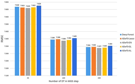
Figure 5. Comparison between the five proposed models on the simulation dataset. In each model, 500 forests with 250 trees are used in the CF step, and 30, 100, and 200 DTs in the MGS step. This comparison includes shrinkage and non-shrinkage techniques. The RMSE is computed for various numbers of decision trees in the multi-grained scanning step.

As illustrated in Figure 6, among the four shrinkage techniques applied to gcforest to decrease trees in the cascade forest step, the EN method demonstrates superior performance. Despite removing fewer trees compared to other shrinkage methods techniques, EN outperforms GL. For this reason, EN selects groups of related trees without grouping them, while the GL method groups the forest. Meanwhile, the AL method has the worst performance due to assigning weight to the penalty function and using the ridge estimator in its weight vector.

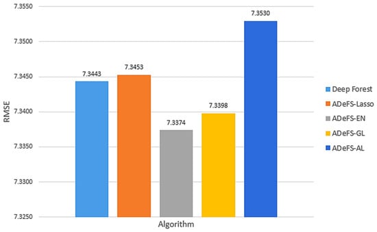
Figure 6. Comparison between the five proposed models on the simulation dataset generated from the linear regression model. In each model, 500 forests with 250 trees are used in the CF step and 200 DTs in the MGS step. This comparison includes shrinkage and non-shrinkage techniques. The RMSE is computed for various numbers of decision trees in the multi-grained scanning step.

5.2. Description of Real Data

The efficacy of the proposed models will be assessed in the current research by using three actual datasets, and the outcomes will be explained. Table 2 provides information on the observations, features, training set, and test set for each dataset. Further details on each dataset are provided below:

Boston Housing Price dataset: This dataset contains information collected by the U.S Census Service concerning housing in the area of Boston Mass. It contains 506 observations and 13 variables with the target variable being the Median value of owner-occupied homes in USD 1000s (MEDV), originally published by Harrison and Rubinfeld [55]. It can also be accessed through the MASS package in R (https://cran.r-project.org/package=MASS (accessed on 7 May 2021)).

Real Estate Valuation dataset: This dataset, sourced from the UCI Machine Learning Repository and originally compiled by Yeh and Hsu [56], includes seven features. Five of these features, namely house age, distance to the nearest MRT station, number of convenience stores in the living circle on foot, latitude, and longitude, along with the transaction date, are selected as independent variables. The target variable is the house price per unit area. The dataset is split into training and test sets, with the training set comprising 332 samples (80%) and the test set comprising 82 samples (20%).

Gold Price per Ounce dataset: The dataset, accessible on GitHub (https://github.com/cominsys/Data_GPPO_01 (accessed on 8 October 2022)), comprises 717 observations and includes four features: high price, low price, open price, and close price. The dataset is treated as time series data. To convert it into a supervised learning problem, the sliding window method [57] is employed. The sliding window method is implemented in several steps. First, the window size, denoted by length k, is determined. Next, the window is slid forward by one unit. This sliding process continues, shifting the window until calculations are conducted window-by-window. This method allows for the sequential analysis of the dataset, facilitating the transformation of the data into a format suitable for supervised learning.

In this study, a window size of 20 is selected, resulting in 80 independent variables and 697 observations. For data preprocessing, the standardization strategy is initially applied. This involves standardizing each feature by subtracting the mean and dividing by the standard deviation:

$$x_{stand}={\displaystyle \frac{x-mean\left(x\right)}{sd\left(x\right)}}$$

(13)

where x represents the sample, mean(.) denotes the mean, and sd(.) illustrates the standard deviation of x. Subsequently, the dataset is split into training and test sets, with the training set comprising 567 samples (80%) and the test set containing 140 samples (20%).

Result of Real Data Analysis

To assess the efficacy of the shrinkage techniques in gcforest, the proposed model is applied to three datasets: Boston housing price, Gold price per ounce, and real estate valuation. For the Boston housing price dataset, which comprises 13 features, the window size in the MGS step is set to 11. In the Gold price per ounce dataset, which includes 80 features, and in the real estate valuation dataset, which contains 5 features, the window sizes are set to 11 and 4, respectively. The number of DTs in the MGS step for all three datasets is set to 30, 100, and 200 trees, and the total number of forests in the CF step is assumed to be 200, 300, and 500 forests. Additionally, 100, 150, and 250 forests are used for each RF and CRF, respectively. The comparison results of the proposed models are presented in Table 5, Table 6 and Table 7, Figure 7a–c and Figure 8a–c.

Table 5. Comparison of the ADeFS model under different combinations with other models on the Boston housing price dataset.

		Models	MSE	RMSE	MAE	Selected Forests
Mgstree = 30	Nforest = 200	Deep forest	10.79664592	3.285824998	2.382859197	200
		ADeFS-Lasso	10.76700983	3.281312211	2.375429196	32
		ADeFS-EN	10.73382078	3.276251026	2.390047538	141
		ADeFS-GL	10.76845759	3.281532812	2.38672813	40
		ADeFS-AL	10.78851201	3.284587039	2.390060198	12
	Nforest = 300	Deep forest	10.76279261	3.280669538	2.380122764	300
		ADeFS-Lasso	10.74056605	3.277280282	2.380369176	33
		ADeFS-EN	10.72747121	3.275281852	2.38187739	163
		ADeFS-GL	10.7324373	3.27603988	2.389402566	40
		ADeFS-AL	10.84499476	3.293173965	2.391307467	11
	Nforest = 500	Deep forest	10.75709129	3.279800496	2.379448729	500
		ADeFS-Lasso	10.73035883	3.275722642	2.387708157	50
		ADeFS-EN	10.67605555	3.267423381	2.37115005	182
		ADeFS-GL	10.72815771	3.27538665	2.375684764	40
		ADeFS-AL	10.85222914	3.294272171	2.388784036	17
Mgstree = 100	Nforest = 200	Deep forest	9.491320519	3.080798682	2.300916575	200
		ADeFS-Lasso	9.489601432	3.080519669	2.326561935	29
		ADeFS-EN	9.447042255	3.073604115	2.297375981	133
		ADeFS-GL	9.488253361	3.080300856	2.302459698	30
		ADeFS-AL	9.763056281	3.124588978	2.341522341	11
	Nforest = 300	Deep forest	9.502236191	3.082569738	2.300884	300
		ADeFS-Lasso	9.49849967	3.081963606	2.301136847	33
		ADeFS-EN	9.479157303	3.078824013	2.302319722	133
		ADeFS-GL	9.481043117	3.079130253	2.339691671	50
		ADeFS-AL	9.680705953	3.111383286	2.311356568	7
	Nforest = 500	Deep forest	9.590581987	3.096866479	2.311685511	500
		ADeFS-Lasso	9.514455975	3.084551179	2.308141017	39
		ADeFS-EN	9.434366409	3.071541373	2.301218161	232
		ADeFS-GL	9.470197823	3.077368652	2.303264279	40
		ADeFS-AL	9.628256009	3.10294312	2.328763889	16
Mgstree = 200	Nforest = 200	Deep forest	9.696804389	3.113969234	2.330913222	200
		ADeFS-Lasso	9.658178965	3.107761086	2.328510577	31
		ADeFS-EN	9.196777517	3.032618921	2.282109635	104
		ADeFS-GL	9.640027169	3.104839315	2.336902901	40
		ADeFS-AL	9.832384856	3.135663384	2.356816707	10
	Nforest = 300	Deep forest	9.706702886	3.115558198	2.329715122	300
		ADeFS-Lasso	9.685857676	3.112211059	2.328584879	38
		ADeFS-EN	9.644626915	3.105579964	2.323499107	128
		ADeFS-GL	9.658178965	3.107761086	2.328510577	30
		ADeFS-AL	9.903258334	3.146944285	2.361301516	9
	Nforest = 500	Deep forest	9.762566823	3.124510653	2.342055087	500
		ADeFS-Lasso	9.689173624	3.112743745	2.334335384	33
		ADeFS-EN	9.59499333	3.097578624	2.323703672	147
		ADeFS-GL	9.672964717	3.110139019	2.331798058	60
		ADeFS-AL	10.03872964	3.168395436	2.376118102	20

Table 6. Comparison of the ADeFS model under different combinations with other models on the Gold price per ounce dataset.

		Models	MSE	RMSE	MAE	Selected Forests
Mgstree = 30	Nforest = 200	Deep forest	0.005088953	0.071336895	0.051698454	200
		ADeFS-Lasso	0.005049879	0.071062498	0.051632094	6
		ADeFS-EN	0.005022097	0.070866758	0.05153941	150
		ADeFS-GL	0.005048572	0.071053303	0.051549264	30
		ADeFS-AL	0.005089575	0.071341257	0.051961681	15
	Nforest = 300	Deep forest	0.005092228	0.071359852	0.051518032	300
		ADeFS-Lasso	0.00506438	0.071164461	0.051610533	6
		ADeFS-EN	0.005046128	0.071036106	0.051559583	216
		ADeFS-GL	0.005056664	0.071110223	0.05167736	30
		ADeFS-AL	0.005117177	0.071534449	0.051955438	16
	Nforest = 500	Deep forest	0.005052299	0.071079525	0.051558663	500
		ADeFS-Lasso	0.005031436	0.070932618	0.051412692	5
		ADeFS-EN	0.005018062	0.070838279	0.051394187	335
		ADeFS-GL	0.005027495	0.07090483	0.051664349	20
		ADeFS-AL	0.005203993	0.072138703	0.051363712	24
Mgstree = 100	Nforest = 200	Deep forest	0.005033754	0.07094895	0.051283147	200
		ADeFS-Lasso	0.005014434	0.070812669	0.051442807	7
		ADeFS-EN	0.004982789	0.070588874	0.051443754	130
		ADeFS-GL	0.005011008	0.070788473	0.051405811	40
		ADeFS-AL	0.005229999	0.072318735	0.052099837	19
	Nforest = 300	Deep forest	0.005072845	0.071223907	0.05092396	300
		ADeFS-Lasso	0.005043856	0.071020112	0.051555775	6
		ADeFS-EN	0.004998525	0.070700249	0.051303172	163
		ADeFS-GL	0.005034941	0.070957321	0.051507318	40
		ADeFS-AL	0.005109748	0.071482498	0.051532747	17
	Nforest = 500	Deep forest	0.005039008	0.070985971	0.051501527	500
		ADeFS-Lasso	0.005078818	0.071265824	0.051722793	9
		ADeFS-EN	0.004991239	0.070648703	0.05081159	140
		ADeFS-GL	0.005020482	0.070855362	0.051505664	50
		ADeFS-AL	0.005139964	0.071693541	0.051856166	18
Mgstree = 200	Nforest = 200	Deep forest	0.005058494	0.07112309	0.051732536	200
		ADeFS-Lasso	0.00505218	0.071078692	0.051659189	6
		ADeFS-EN	0.005030576	0.070926555	0.051470238	176
		ADeFS-GL	0.005051513	0.071073996	0.051677736	30
		ADeFS-AL	0.005112947	0.071504874	0.052009983	15
	Nforest = 300	Deep forest	0.005090297	0.071346317	0.051969626	300
		ADeFS-Lasso	0.005089528	0.07134093	0.051966418	9
		ADeFS-EN	0.005041552	0.071003886	0.051572782	186
		ADeFS-GL	0.005049189	0.071057646	0.0517376	30
		ADeFS-AL	0.005162974	0.071853837	0.051246741	19
	Nforest = 500	Deep forest	0.005046643	0.071039731	0.051724809	500
		ADeFS-Lasso	0.005045004	0.07102819	0.05194221	11
		ADeFS-EN	0.005035997	0.07096476	0.051855762	217
		ADeFS-GL	0.005037518	0.070975473	0.051709537	60
		ADeFS-AL	0.005077337	0.071255433	0.051084327	19

Table 7. Comparison of the ADeFS model under different combinations with other models on the real estate valuation dataset.

		Models	MSE	RMSE	MAE	Selected Forests
Mgstree = 30	Nforest = 200	Deep forest	31.21329454	5.586885943	4.18779841	200
		ADeFS-Lasso	31.20524607	5.586165596	4.187668722	41
		ADeFS-EN	30.98465652	5.566386307	4.16904536	109
		ADeFS-GL	31.11342701	5.577941109	4.176917527	40
		ADeFS-AL	31.26858715	5.591832182	4.21386215	16
	Nforest = 300	Deep forest	31.04979611	5.57224466	4.188160332	300
		ADeFS-Lasso	31.04879681	5.572134454	4.190314497	49
		ADeFS-EN	30.92550847	5.561070802	4.193493422	122
		ADeFS-GL	31.02130065	5.569676889	4.191075998	50
		ADeFS-AL	31.07623278	5.574606065	4.18375101	19
	Nforest = 500	Deep forest	31.09472813	5.576264712	4.194908917	500
		ADeFS-Lasso	31.03552387	5.570953587	4.187729141	48
		ADeFS-EN	30.7947445	5.549301263	4.196798411	237
		ADeFS-GL	30.86627945	5.555742925	4.186367565	40
		ADeFS-AL	31.29315788	5.59402877	4.171925183	18
Mgstree = 100	Nforest = 200	Deep forest	32.93931402	5.73927818	4.345550696	200
		ADeFS-Lasso	32.89762888	5.73564546	4.335513676	45
		ADeFS-EN	32.87191329	5.73340329	4.349156282	62
		ADeFS-GL	32.8792486	5.73404295	4.346583843	50
		ADeFS-AL	32.90043853	5.73589039	4.331290279	13
	Nforest = 300	Deep forest	33.2270951	5.764294849	4.354197238	300
		ADeFS-Lasso	32.9459494	5.739856218	4.348453524	50
		ADeFS-EN	32.67427974	5.716142033	4.334556292	177
		ADeFS-GL	32.92069902	5.737656231	4.347547327	40
		ADeFS-AL	33.1667478	5.759057892	4.378162328	14
	Nforest = 500	Deep forest	33.09941777	5.753209345	4.356595739	500
		ADeFS-Lasso	33.02598134	5.746823587	4.357942156	53
		ADeFS-EN	32.71775085	5.719943256	4.329941517	220
		ADeFS-GL	32.2787384	5.681438057	4.33582318	40
		ADeFS-AL	33.40171361	5.779421564	4.369489994	17
Mgstree = 200	Nforest = 200	Deep forest	28.31477232	5.321162685	4.163856615	200
		ADeFS-Lasso	28.2847825	5.318343962	4.161216924	58
		ADeFS-EN	28.21039753	5.311346113	4.163218212	140
		ADeFS-GL	28.25655969	5.315689955	4.170575129	60
		ADeFS-AL	28.58312519	5.346318844	4.196550904	13
	Nforest = 300	Deep forest	28.39429433	5.328629686	4.165342895	300
		ADeFS-Lasso	28.204044	5.31074797	4.157510565	50
		ADeFS-EN	27.99934435	5.291440668	4.1440135	139
		ADeFS-GL	28.20152376	5.310510687	4.153345482	30
		ADeFS-AL	28.3956606	5.328757886	4.151699603	15
	Nforest = 500	Deep forest	28.3160343	5.321281265	4.147863948	500
		ADeFS-Lasso	28.16257631	5.306842404	4.15521972	77
		ADeFS-EN	28.14859982	5.305525405	4.14459601	196
		ADeFS-GL	28.15036776	5.305692015	4.149334811	40
		ADeFS-AL	28.32922216	5.322520283	4.141166132	18

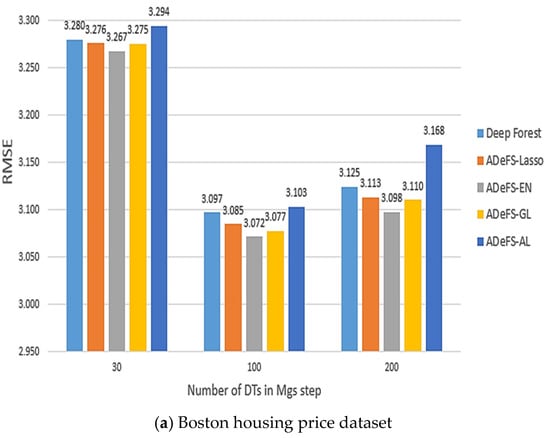
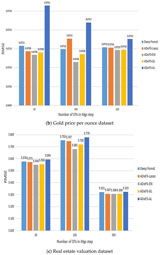
Figure 7. Comparison between the five proposed models on the simulation dataset. In each model, 500 forests are used in the CF step and 30, 100, and 200 DTs in the MGS step. This comparison includes shrinkage and non-shrinkage techniques.

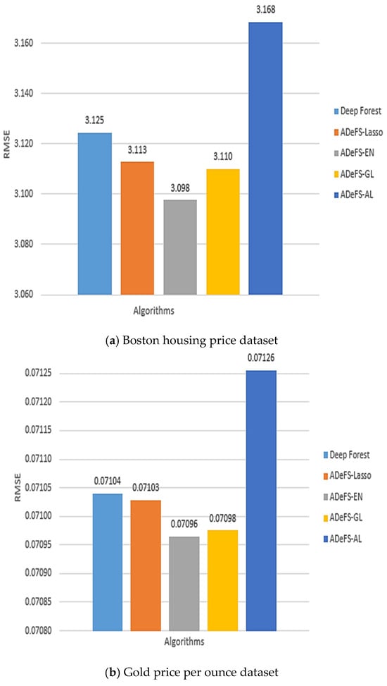
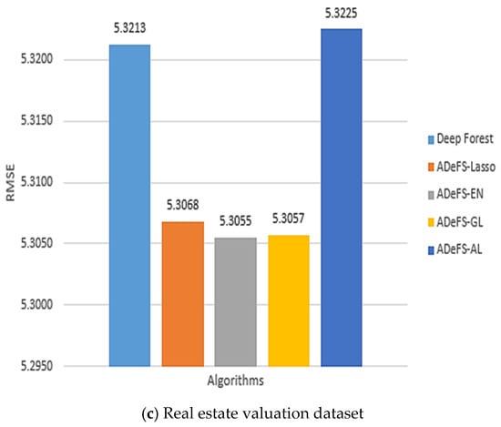
Figure 8. Comparison between the five proposed models on the simulation dataset generated from the linear regression model. In each model, 500 forests are used in the CF step and 200 DTs in the MGS step. This comparison includes shrinkage and non-shrinkage techniques.

According to Table 5, Table 6 and Table 7, which show the comparison results of the proposed model on the Boston housing price, Gold price per ounce, and real estate valuation datasets, respectively, applying EN to reduce the number of forests in CF step in gcforest algorithm outperforms. Table 5 shows the obtained results of the Boston housing price dataset. Increasing the number of DTs from 30 trees to 200 trees in the MGS step, the MSE, RMSE, and MAE decrease from 10.6760, 3.2674, and 2.3711 to 9.5949, 3.0975, and 2.3237 in the ADeFS-EN model, respectively. When 500 forests are used in the CF step, the ADeFS-AL model, which has the worst performance among the proposed models, achieves a decrease in error values based on the MSE, RMSE, and MAE criteria from 10.8522, 3.2942, and 2.3887 to 10.038, 3.1683, and 2.3761, respectively. Meanwhile, in the other two datasets used in this study, ADeFS-EN outperforms the other models.

Figure 8a–c depict the outcomes of the proposed model, specifically focusing on the RMSE metric, utilizing 200 DTs in the MGS step and 500 forests in the CF step. The plots illustrate that the ADeFS-EN model outperforms other models in all three datasets in terms of RMSE, while the ADeFS-AL model presents the worst performance. This means that not only applying shrinkage techniques on the forests of the last layer in the CF step can improve the performance, but also the type of shrinkage technique is effective in further reducing the error. For example, the EN method, which simultaneously shrinks and selects the forests and performs group selection, outperforms. Although the ADeFS-EN model keeps more forests in the model, it still achieves better performance. This can be attributed to the penalty function, which combines the characteristics of ridge and LASSO regression. It receives both the shrinkage property from ridge and the property of removing them from Lasso. On the other hand, the GL method carries out group selection but does not perform better than EN. This is because the grouping of forests may lead to removing an effective group of forests from the model, resulting in higher model error.

As previously discussed, increasing the number of DTs in the MGS step enhances our model’s performance, whereas increasing the number of forests in the CF step, from 200 to 500, results in an increase in the error rate. For example, in the Boston housing price dataset, the gcforest error rises from 9.6968, 3.1139, and 2.3309 to 9.7625, 3.1245, and 3.3420 based on the MSE, RMSE, and MAE criteria, respectively. However, by applying the methods and automatically reducing the number of trees, the error rate in the proposed ADeFS-EN model increases from 9.1967, 3.0326, and 2.02821 to 9.5949, 3.0975, and 2.3237. Despite an increase in error as the number of trees grows following the application of shrinkage techniques, the resulting error remains lower compared to the model without shrinkage techniques.

6. Discussion

Deep neural networks have a significant number of hyperparameters, and the learning performance is highly dependent on the careful tuning of these parameters. The complexity and computational load are reduced by decreasing the number of hyperparameters. Currently, deep forest regression architecture has shown remarkable success in prediction. One notable advantage of DF is its ability to integrate the DL and RF theory in the prediction process. Another advantage is its adaptive determination of the number of cascade levels, automatically setting the model’s complexity while the number of trees and forests are selected by the user. Users can leverage various types of algorithms, such as RF, CRF, LightGBM, Extra trees, and XGboost, in cascade forests. In the present study, a new hybrid deep forest was proposed, utilizing shrinkage techniques to automatically remove ineffective forests and trees. This not only increased prediction accuracy but also reduced the model’s complexity and computational load by minimizing hyperparameters. In previous research, shrinkage techniques were utilized to decrease the number of trees in RF, while in the present research, shrinkage techniques were employed to automatically decrease the number of forests in the DF algorithm.

The proposed model’s performance is assessed by comparing its results on the three datasets with those obtained by previous models. The results are given in Table 8, Table 9 and Table 10 with 500 trees in RF and 500 forests in the CF step and 200 trees in the MGS step of DF. According to Table 8, in the Boston housing price dataset, the proposed ADeFS-EN model, which was a combination of the gcforest algorithm and shrinkage techniques, achieved the highest accuracy compared to RARTEN, ECAPRAF, and PBRF which was a combination of the RF algorithm and shrinkage techniques. Similarly, in the real estate valuation and Gold price per ounce datasets, as shown, respectively, in Table 9 and Table 10, the current proposed model performed significantly better than the other three methods. In all the previous models as well as in the new proposed model, the combination of machine learning and deep learning algorithms with the EN shrinkage technique outperformed the original algorithms because EN can keep the most effective trees in the model by combining the ridge and lasso methods. On the other hand, due to the presence of the ridge estimator in the denominator of the weight vector, the penalty function in AL is increased, leading to an error rise. Therefore, combining the EN method with algorithms like RF and DF provided better performance than the other combined models.

Table 8. Comparison results of the ADeFS model with previous models on the Boston housing price dataset.

Models	MSE	RMSE	MAE	No. of Selected Trees
PBRF [58]	9.815481693	3.132966915	2.122203605	85
RARTEN [7]	9.735025589	3.120100253	2.090654468	120
ECAPRAF-EN [6]	10.55174201	3.248344504	2.157154185	106
ADeFS-EN(Ours)	9.59499333	3.097578624	2.323703672	147

Table 9. Comparison results of the ADeFS model with previous models on the real estate valuation dataset.

Models	MSE	RMSE	MAE	No. of Selected Trees
PBRF [58]	105.5873882	10.2755724	5.250650213	200
RARTEN [7]	105.303779	10.26176296	5.281261517	66
ECAPRAF-EN [6]	30.33592275	5.507805621	4.207588771	111
ADeFS-EN(Ours)	28.14859982	5.305525405	4.14459601	196

Table 10. Comparison results of the ADeFS model with previous models on the Gold price per ounce.

Models	MSE	RMSE	MAE	No. of Selected Trees
PBRF [58]	0.006211212	0.078811245	0.054854592	57
RARTEN [7]	0.006209254	0.078798823	0.054633005	171
ECAPRAF-EN [6]	0.005327555	0.072990105	0.049057753	234
ADeFS-EN(Ours)	0.005035997	0.07096476	0.051855762	217

The results of comparing three data with 500 trees, as presented in Table 8, Table 9 and Table 10, indicate that the ECAPRAF model performed better than PBRF and RARTEN. Furthermore, the ADeFS-EN achieved an error rate that outperformed ECAPRAF-EN and PBRF. Although ECAPRAF-EN performed better than the PBRF and RARTEN models, it had lower performance compared to our proposed model in this paper. Since the new proposed model uses DF instead of RF, its performance is better than RF. The new proposed model can compete with recent models by achieving the lowest error.

7. Conclusions

To reduce computational load and minimize errors in the prediction phase, a hybrid model can be created by combining statistical methods and artificial intelligence algorithms. In this study, a model consisting of four steps was developed, which performs better than previous models. In the first step, a sliding window was employed to extract the relationship between input features which led to the production of feature vectors. These vectors were used to construct RF and CRF. In the second step, the CF was divided into different levels based on the extracted features from the previous step. Within each level, multiple random forests were used to perform prediction at this step. Considering a large number of forests, gcforest does not have appropriate performance. Therefore, its performance was improved by reducing the number of forests through the use of shrinking methods. The shrinkage techniques that were employed to reduce the number of forests include Lasso, EN, GL, and AL. The remaining trees were aggregated, and ensembling was performed for the final prediction using simple average methods. The performance of our proposed model was evaluated by three real datasets and one simulated dataset. Then, the results were compared based on the MSE, RMSE, and MAE criteria. The findings indicated that the ADeFS-EN model, which is a combination of gcforest and EN, outperforms the other models. Moreover, as the number of MGS step DT and CF step increases, ADeFS-EN continues to outperform the other models.

References

- Li, G.; Ma, H.-D.; Liu, R.-Y.; Shen, M.-D.; Zhang, K.-X. A Two-Stage Hybrid Default Discriminant Model Based on Deep Forest. Entropy 2021, 23, 582. [Google Scholar] [CrossRef]
- Zeng, Y.; Chen, H.; Xu, C.; Cheng, Y.; Gong, Q. A hybrid deep forest approach for outlier detection and fault diagnosis of variable refrigerant flow system. Int. J. Refrig. 2020, 120, 104–118. [Google Scholar] [CrossRef]
- He, D.; Li, C.; Chen, Y.; Li, X. Prediction of thermal conductivity of hybrid nanofluids based on deep forest model. Heat Transf. Res. 2022, 53, 55–71. [Google Scholar] [CrossRef]
- Dong, Y.; Yang, W.; Wang, J.; Zhao, J.; Qiang, Y. MLW-gcForest: A Multi-Weighted gcForest Model for Cancer Subtype Classification by Methylation Data. Appl. Sci. 2019, 9, 3589. [Google Scholar] [CrossRef]
- Dong, Y.; Yang, W.; Wang, J.; Zhao, J.; Qiang, Y.; Zhao, Z.; Kazihise, N.G.F.; Cui, Y.; Yang, X.; Liu, S. MLW-gcForest: A multi-weighted gcForest model towards the staging of lung adenocarcinoma based on multi-modal genetic data. BMC Bioinform. 2019, 20, 578. [Google Scholar] [CrossRef]
- Farhadi, Z.; Bevrani, H.; Feizi-Derakhshi, M.R.; Kim, W.; Ijaz, M.F. An Ensemble Framework to Improve the Accuracy of Prediction Using Clustered Random-Forest and Shrinkage Methods. Appl. Sci. 2022, 12, 10608. [Google Scholar] [CrossRef]
- Farhadi, Z.; Bevrani, H.; Feizi-Derakhshi, M.R. Improving random forest algorithm by selecting appropriate penalized method. Commun. Stat.-Simul. Comput. 2022, 53, 4380–4395. [Google Scholar] [CrossRef]
- Farhadi, Z.; Feizi-Derakhshi, M.R.; Bevrani, H.; Kim, W.; Ijaz, M.F. ERDeR: The combination of statistical shrinkage methods and ensemble approaches to improve the performance of deep regression. IEEE Access 2024, 12, 33361–33383. [Google Scholar] [CrossRef]
- Goodfellow, I.; Bengio, Y.; Courville, A. Deep Learning; MIT Press: Cambridge, MA, USA, 2016; ISBN 978-0262035613. [Google Scholar]
- Al-Tameemi, I.K.S.; Feizi-Derakhshi, M.-R.; Pashazadeh, S.; Asadpour, M. Interpretable Multimodal Sentiment Classification Using Deep Multi-View Attentive Network of Image and Text Data. IEEE Access 2023, 11, 91060–91081. [Google Scholar] [CrossRef]
- Gawlikowski, J.; Tassi, C.R.N.; Ali, M.; Lee, J.; Humt, M.; Feng, J.; Kruspe, A.; Triebel, R.; Jung, P.; Roscher, R.; et al. A survey of uncertainty in deep neural networks. Artif. Intell. Rev. 2023, 56, 1513–1589. [Google Scholar] [CrossRef]
- Reyad, M.; Sarhan, A.M.; Arafa, M. A modified Adam algorithm for deep neural network optimization. Neural Comput. Appl. 2023, 35, 17095–17112. [Google Scholar] [CrossRef]
- Zhou, Z.H.; Feng, J. Deep forest. Natl. Sci. Rev. 2019, 6, 74–86. [Google Scholar] [CrossRef]
- Datta, D.; Mallick, P.K.; Reddy, A.V.N.; Mohammed, M.A.; Jaber, M.M.; Alghawli, A.S.; Al-qaness, M.A.A. A Hybrid Classification of Imbalanced Hyperspectral Images Using ADASYN and Enhanced Deep Subsampled Multi-Grained Cascaded Forest. Remote Sens. 2022, 14, 4853. [Google Scholar] [CrossRef]
- Choi, K.S.; Shin, J.S.; Lee, J.J.; Kim, Y.S.; Kim, S.B.; Kim, C.W. In vitro trans-differentiation of rat mesenchymal cells into insulin-producing cells by rat pancreatic extract. Biochem. Biophys. Res. Commun. 2005, 330, 1299–1305. [Google Scholar] [CrossRef] [PubMed]
- Krizhevsky, A.; Sutskever, I.; Hinton, G.E. ImageNet classification with deep convolutional neural networks. Commun. ACM 2017, 60, 84–90. [Google Scholar] [CrossRef]
- Breiman, L. Random Forests. Mach. Learn. 2001, 45, 5–32. [Google Scholar] [CrossRef]
- Wang, H.; Tang, Y.; Jia, Z.; Ye, F. Dense adaptive cascade forest: A self-adaptive deep ensemble for classification problems. Soft Comput. 2020, 24, 2955–2968. [Google Scholar] [CrossRef]
- Ghaemi, M.; Feizi-Derakhshi, M.-R. Feature selection using Forest Optimization Algorithm. Pattern Recognit. 2016, 60, 121–129. [Google Scholar] [CrossRef]
- Ghaemi, M.; Feizi-Derakhshi, M.-R. Forest Optimization Algorithm. Expert Syst. Appl. 2014, 41, 6676–6687. [Google Scholar] [CrossRef]
- Zhang, W.; Xue, Z.; Li, Z.; Yin, H. DCE-DForest: A Deep Forest Model for the Prediction of Anticancer Drug Combination Effects. Comput. Math. Methods Med. 2022, 2022, 8693746. [Google Scholar] [CrossRef]
- Wu, L.; Gao, J.; Zhang, Y.; Sui, B.; Wen, Y.; Wu, Q.; Liu, K.; He, S.; Bo, X. A hybrid deep forest-based method for predicting synergistic drug combinations. Cell Rep. Methods 2023, 3, 100411. [Google Scholar] [CrossRef] [PubMed]
- Jin, W.; Stokes, J.M.; Eastman, R.T.; Itkin, Z.; Zakharov, A.V.; Collins, J.J.; Jaakkola, T.S.; Barzilay, R. Deep learning identifies synergistic drug combinations for treating COVID-19. Proc. Natl. Acad. Sci. USA 2021, 118, e2105070118. [Google Scholar] [CrossRef] [PubMed]
- Ding, J.; Luo, Q.; Jia, L.; You, J. Deep Forest-Based Fault Diagnosis Method for Chemical Process. Math. Probl. Eng. 2020, 2020, 5281512. [Google Scholar] [CrossRef]
- Jiao, Z.; Hu, P.; Xu, H.; Wang, Q. Machine Learning and Deep Learning in Chemical Health and Safety: A Systematic Review of Techniques and Applications. ACS Chem. Health Saf. 2020, 27, 316–334. [Google Scholar] [CrossRef]
- AlJame, M.; Imtiaz, A.; Ahmad, I.; Mohammed, A. Deep forest model for diagnosing COVID-19 from routine blood tests. Sci. Rep. 2021, 11, 16682. [Google Scholar] [CrossRef] [PubMed]
- Singh, D.; Kumar, V.; Kaur, M.; Kumari, R. Early diagnosis of COVID-19 patients using deep learning-based deep forest model. J. Exp. Theor. Artif. Intell. 2023, 35, 365–375. [Google Scholar] [CrossRef]
- Modi, P.; Kumar, Y. Smart detection and diagnosis of diabetic retinopathy using bat based feature selection algorithm and deep forest technique. Comput. Ind. Eng. 2023, 182, 109364. [Google Scholar] [CrossRef]
- Yin, L.; Sun, Z.; Gao, F.; Liu, H. Deep Forest Regression for Short-Term Load Forecasting of Power Systems. IEEE Access 2020, 8, 49090–49099. [Google Scholar] [CrossRef]
- Wu, T.; Zhao, Y.; Liu, L.; Li, H.; Xu, W.; Chen, C. A novel hierarchical regression approach for human facial age estimation based on deep forest. In Proceedings of the 2018 IEEE 15th International Conference on Networking, Sensing and Control (ICNSC), Zhuhai, China, 27–29 March 2018; pp. 1–6. [Google Scholar] [CrossRef]
- Simonyan, K.; Zisserman, A. Very deep convolutional networks for large-scale image recognition. In Proceedings of the 3rd International Conference on Learning Representation, ICLR 2015, San Diego, CA, USA, 7–9 May 2015; pp. 1–14. [Google Scholar]
- Shen, W.; Guo, Y.; Wang, Y.; Zhao, K.; Wang, B.; Yuille, A. Deep Regression Forests for Age Estimation. In Proceedings of the IEEE Conference on Computer Vision and Pattern Recognition (CVPR), Salt Lake City, UT, USA, 18–23 June 2018; pp. 2304–2313. Available online: http://hdl.handle.net/1721.1/115413 (accessed on 22 December 2024).
- Guo, Y.; Liu, S.; Li, Z.; Shang, X. BCDForest: A boosting cascade deep forest model towards the classification of cancer subtypes based on gene expression data. BMC Bioinform. 2018, 19, 118. [Google Scholar] [CrossRef] [PubMed]
- Sun, L.; Mo, Z.; Yan, F.; Xia, L.; Shan, F.; Ding, Z.; Song, B.; Gao, W.; Shao, W.; Shi, F.; et al. Adaptive Feature Selection Guided Deep Forest for COVID-19 Classification with Chest CT. IEEE J. Biomed. Health Inform. 2020, 24, 2798–2805. [Google Scholar] [CrossRef] [PubMed]
- Lin, W.; Wu, L.; Zhang, Y.; Wen, Y.; Yan, B.; Dai, C.; Liu, K.; He, S.; Bo, X. An Enhanced Cascade-Based Deep Forest Model for Drug Combination Prediction. Brief. Bioinform. 2022, 23, bbab562. [Google Scholar] [CrossRef]
- Xia, H.; Tang, J. An Improved Deep Forest Regression. In Proceedings of the 2021 3rd International Conference on Industrial Artificial Intelligence (IAI), Shenyang, China, 8–11 November 2021; pp. 1–6. [Google Scholar]
- Liu, F.T.; Ting, K.M.; Zhou, Z.H. Isolation forest. In Proceedings of the 2008 Eighth IEEE International Conference on Data Mining, Pisa, Italy, 15–19 December 2008; pp. 413–422. [Google Scholar] [CrossRef]
- Zhou, Y.; Chen, J.; Yu, Z.J.; Li, J.; Huang, G.; Haghighat, F.; Zhang, G. A novel model based on multi-grained cascade forests with wavelet denoising for indoor occupancy estimation. Build. Environ. 2020, 167, 106461. [Google Scholar] [CrossRef]
- Chen, C.; Liu, Y.; Sun, X.; Di Cairano-Gilfedder, C.; Titmus, S. Automobile Maintenance Modelling Using gcForest. In Proceedings of the 2020 IEEE 16th International Conference on Automation Science and Engineering (CASE), Hong Kong, China, 20–21 August 2020; pp. 600–605. [Google Scholar] [CrossRef]
- Chu, Y.; Kaushik, A.C.; Wang, X.; Wang, W.; Zhang, Y.; Shan, X.; Salahub, D.R.; Xiong, Y.; Wei, D.-Q. DTI-CDF: A cascade deep forest model towards the prediction of drug-target interactions based on hybrid features. Brief. Bioinform. 2021, 22, 451–462. [Google Scholar] [CrossRef] [PubMed]
- Chen, Y.; Guo, A.; Chen, Q.; Quan, B.; Liu, G.; Li, L.; Hong, J.; Wei, H.; Hao, Z. Intelligent classification of antepartum cardiotocography model based on deep forest. Biomed. Signal Process. Control. 2021, 67, 102555. [Google Scholar] [CrossRef]
- Liu, W.; Lin, H.; Huang, L.; Peng, L.; Tang, T.; Zhao, Q.; Yang, L. Identification of miRNA–disease associations via deep forest ensemble learning based on autoencoder. Brief. Bioinform. 2022, 23, bbac104. [Google Scholar] [CrossRef] [PubMed]
- Li, D.; Liu, Z.; Armaghani, D.J.; Xiao, P.; Zhou, J. Novel Ensemble Tree Solution for Rockburst Prediction Using Deep Forest. Mathematics 2022, 10, 787. [Google Scholar] [CrossRef]
- Yu, B.; Chen, C.; Wang, X.; Yu, Z.; Ma, A.; Liu, B. Prediction of protein–protein interactions based on elastic net and deep forest. Expert Syst. Appl. 2021, 176, 114876. [Google Scholar] [CrossRef]
- Li, Q.; Wang, Y.; Du, Z.; Li, Q.; Zhang, W.; Zhong, F.; Wang, Z.J.; Chen, Z. APDF: An active preference-based deep forest expert system for overall survival prediction in gastric cancer. Expert Syst. Appl. 2024, 245, 123131. [Google Scholar] [CrossRef]
- Chen, T.; Guestrin, C. XGBoost: A scalable tree boosting system. In Proceedings of the 22nd ACM SIGKDD International Conference on Knowledge Discovery and Data Mining, San Francisco, CA, USA, 13–17 August 2016; pp. 785–794. [Google Scholar] [CrossRef]
- Farhadi, Z.; Arabi Belaghi, R.; Gurunlu Alma, O. Analysis of Penalized Regression Methods in a Simple Linear Model on the High-Dimensional Data. Am. J. Theor. Appl. Stat. 2019, 8, 185–192. [Google Scholar] [CrossRef]
- Hirose, K.; Terada, Y. Sparse and Simple Structure Estimation via Prenet Penalization. Psychometrika 2023, 88, 1381–1406. [Google Scholar] [CrossRef] [PubMed]
- Tibshirani, R. Regression Shrinkage and Selection via the Lasso. J. R. Stat. Society. Ser. B (Methodol.) 1996, 58, 267–288. Available online: http://www.jstor.org/stable/2346178 (accessed on 22 December 2024). [CrossRef]
- Liu, X.; Meng, X.; Wang, X. Carbon Emissions Prediction of Jiangsu Province Based on Lasso-BP Neural Network Combined Model. IOP Conf. Ser. Earth Environ. Sci. 2021, 769, 022017. [Google Scholar] [CrossRef]
- Zou, H.; Hastie, T. Regularization and variable selection via the elastic net. J. R. Stat. Soc. Ser. B Stat. Methodol. 2005, 67, 301–320. [Google Scholar] [CrossRef]
- Hoerl, A.E.; Kennard, R.W. Ridge Regression: Biased Estimation for Nonorthogonal Problems. Technometrics 1970, 12, 55–67. [Google Scholar] [CrossRef]
- Zou, H. The adaptive lasso and its oracle properties. J. Am. Stat. Assoc. 2006, 101, 1418–1429. [Google Scholar] [CrossRef]
- Yuan, M.; Lin, Y. Model selection and estimation in regression with grouped variables. J. R. Stat. Soc. Ser. B Stat. Methodol. 2006, 68, 49–67. [Google Scholar] [CrossRef]
- Harrison, D.; Rubinfeld, D.L. Hedonic housing prices and the demand for clean air. J. Environ. Econ. Manag. 1978, 5, 81–102. [Google Scholar] [CrossRef]
- Yeh, I.-C.; Hsu, T.-K. Building real estate valuation models with comparative approach through case-based reasoning. Appl. Soft Comput. 2018, 65, 260–271. [Google Scholar] [CrossRef]
- Chu, C.-S.J. Time series segmentation: A sliding window approach. Inf. Sci. 1995, 85, 147–173. [Google Scholar] [CrossRef]
- Wang, H.; Wang, G. Improving random forest algorithm by Lasso method. J. Stat. Comput. Simul. 2020, 91, 353–367. [Google Scholar] [CrossRef]
Disclaimer/Publisher’s Note: The statements, opinions and data contained in all publications are solely those of the individual author(s) and contributor(s) and not of MDPI and/or the editor(s). MDPI and/or the editor(s) disclaim responsibility for any injury to people or property resulting from any ideas, methods, instructions or products referred to in the content. |
© 2024 by the authors. Licensee MDPI, Basel, Switzerland. This article is an open access article distributed under the terms and conditions of the Creative Commons Attribution (CC BY) license (https://creativecommons.org/licenses/by/4.0/).