Isolation Number of Transition Graphs

Abstract

Let $G=(V,E)$ be a graph and $\mathcal{F}$ be a family of graphs; a subset ($S\subseteq V\left(G\right)$) is said to be an $\mathcal{F}$-isolating set if $G[V\left(G\right)\setminus N_G\left[S\right]]$ does not contain F as a subgraph for all $F\in \mathcal{F}$. The $\mathcal{F}$-isolation number of G is the minimum cardinality of an $\mathcal{F}$-isolating set (S) of G, denoted by $\iota (G,\mathcal{F})$. When $\mathcal{F}=\left\{K_{1,k+1}\right\}$, we use ${\iota }_k\left(G\right)$ to define the $\mathcal{F}$-isolation number ($\iota (G,\mathcal{F})$). In particular, when $k=0$, we use the short form of $\iota \left(G\right)$ instead of ${\iota }_0\left(G\right)$. A subset ($S\subseteq V\left(G\right)$) is called an isolating set if $V\left(G\right)\setminus N_G\left[S\right]$ is an independent set of G. The isolation number of G is the minimum cardinality of an isolating set, denoted by $\iota \left(G\right)$. In this paper, we mainly focus on research on the isolation number and $\mathcal{F}$-isolation number of a $B\left(G\right)$ graph, total graph and central graph of graph G.

1. Introduction

For graph theoretic terminology, we refer to [1,2,3,4]. Let $G=(V,E)$ be a graph with a vertex set ($V=V\left(G\right)$) of order $n\left(G\right)=\left|V\right|$ and an edge set ($E=E\left(G\right)$) of size $m\left(G\right)=\left|E\right|$. For $X,Y\subseteq G$, let $E(X,Y)$ be the number of edges between X and Y in G. Let $G\left[X\right]$ denote the induced subgraph of X in G. For each vertex ($v\in V\left(G\right)$), the degree ($d_G\left(v\right)$) of v is the number of neighbors of v in G. $\Delta \left(G\right)$ ($\delta \left(G\right)$) denotes the maximum (minimum) degree of G. The open neighborhood ($N\left(v\right)$) of a vertex (v) in G is the set of neighbors of v, and the closed neighborhood ($N\left[v\right]$) of v is $N\left(v\right)\cup \left\{v\right\}$. For a subset ($S\subseteq V\left(G\right)$), the open neighborhood of S is the set expressed as $N\left(S\right)={\displaystyle \bigcup _{v\in S}}{N}_G\left(v\right)$, and the closed neighborhood of S is the set expressed as $N\left[S\right]=N\left(S\right)\cup S$. $G\setminus S$ represents the subgraph of G obtained by deleting the vertices of S and all edges incident to all vertices of S. The path, the cycle, the star and the complete graph of order n are written as $P_n$, $C_n$, $S_n$ and $K_n$, respectively. The complete bipartite graph and the complete multipartite graph are written as $K_{m,n}$ and $K_{1,2,\dots k}$, respectively.

For a vertex subset (S) of G, S is a $dominating$ $set$ of G if $N_G\left[S\right]=V\left(G\right)$. The $domination$ $number$ ($\gamma \left(G\right)$) of G is the minimum cardinality of a dominating set of G, that is, $\gamma \left(G\right)=min\left\{\right|S|:SisadominatingsetofG\}$.

For an integer (k), if $\mathcal{F}=\left\{K_k\right\}$, the size of a minimum $K_k$-isolating set of G is denoted by $\iota (G,k)$. The k-$isolation$ $number$ is the minimum cardinality of an $\mathcal{F}$-isolating set (S) of G if $\mathcal{F}=\left\{K_{1,k+1}\right\}$, denoted by ${\iota }_k\left(G\right)$. In particular, a subset ($S\subseteq V$) is called an $isolating$ $set$ of G if $G[V\setminus N_G\left[S\right]]$ has no edge. We define set $R\left(S\right)$ as set $V\left(G\right)\setminus N_G\left[S\right]$. Therefore, a set ($S\subseteq V$) is said to be an isolating set if $R\left(S\right)$ is an independent set of G. The $isolation$ $number$ is the minimum cardinality of an isolating set (S) of G, denoted by $\iota \left(G\right)$. Obviously, if $\mathcal{F}=\left\{K_1\right\}$, S is a dominating set of G.

In 1958, Berge [1] first proposed the concept of the domination number. Many scholars have great research interest in domination theory in graphs, mostly due to its application in many research fields, such as genetics [5], chemistry [6], computer communication networks [7], facility location [8], social networks [9], etc. With the deepening of research, scholars have found that although classical domination theory can solve many practical problems, many solutions that rely only on dominating sets are not optimal solutions to solve problems. As a result, various domination variants are constantly proposed. Partial domination is one of the more widely used approaches. The study of isolating sets was introduced by Caro and Hansberg. In 2015, Caro and Hansberg [10] extended domination to partial domination and proposed the concept of an $\mathcal{F}$-isolating set of graphs for the first time. Results of research on the isolation number can be found in [11,12,13,14,15,16,17,18,19,20]. On the basis of this research, in this paper, we mainly focus on research on the isolation number and $\mathcal{F}$-isolation number of a $B\left(G\right)$ graph, total graph and central graph of graph G.

Definition 1. 

Given a graph (G) with a vertex set of $V\left(G\right)$ = $\left\{v_1,v_2,\dots ,v_n\right\}$, we define a bipartite graph ($B\left(G\right)$) of G in the following way. Let $V_1=\left\{v_1^1,v_2^1,\dots ,v_n^1\right\}$ and $V_2=\left\{v_1^2,v_2^2,\dots ,v_n^2\right\}$ be two partite sets of $B\left(G\right)$, and for $i,j\in \left\{1,2,\dots ,n\right\}$, let $v_i^1$ be adjacent to $v_j^2$ if and only if either $i=j$ or $v_i$ is adjacent to $v_j$ in G. Note that $\left|V\right(B\left(G\right)\left)\right|=2n$, |E(B(G))|=3n − 2 and $d_G\left(v^1\right)=d_G\left(v^2\right)=d_G\left(v\right)+1$ for each $v\in V\left(G\right)$ (Figure 1).

Definition 2 

([21]). Let G be a graph with vertex set $V\left(G\right)$ and edge set $E\left(G\right)$; a total graph ($T\left(G\right)$) of G is a graph in which vertex set $V\left(T\right(G\left)\right)$ is $V\cup E$ and two vertices in $T\left(G\right)$ are adjacent whenever they are either adjacent or incident in G. In the proof below, let $V\left(G\right)=\{v_1,v_2,\dots ,v_n\}$ and $V\left(T\left(G\right)\right)=V\left(G\right)\cup V^{\prime }$ comprise the vertex set of $T\left(G\right)$ in which $V^{\prime }=\left\{v_{ij}\right|v_i{v}_j\in E\left(G\right)\}$ for $1\le i\le j\le n$ (Figure 2).

Definition 3 

([22]). For a graph ($G=(V,E)$) with order n and size m, the central graph of G denoted by $C\left(G\right)$ is a graph of order $n+m$ and size $\left({\displaystyle \genfrac{}{}{0pt}{}{n}{2}}\right)+m$, which is obtained by subdividing each edge of G exactly once and joining all the non-adjacent vertices of G in $C\left(G\right)$. In this section, assume that $V\left(G\right)=\{v_1,v_2,\dots ,v_n\}$ is the vertex set of G and $V\left(C\right(G\left)\right)=V\left(G\right)\cup \mathcal{C}$ is the vertex set of $C\left(G\right)$, where $\mathcal{C}=\left\{c_{ij}\right|v_i{v}_j\in E\left(G\right)\}$ (Figure 3).

Definition 4. 

A spanning tree of a graph G is said to be a BFS tree rooted at a vertex r if and only if, for any vertex (u) of G, the shortest distance between r and u in G is equal to the shortest distance between r and u in the spanning tree. It starts at the root and searches all vertices of G at the current depth level before moving on to the vertex at the next depth level (Figure 4).

The BFS tree is also a breadth-first search tree, which is essentially a spanning tree of the graph. In fact, the purpose of the BFS tree is to determine a vertex from the graph and traverse all vertices of the graph layer by layer from this vertex. Each connected graph has a BFS tree.

Lemma 1 

([23]). Let G be an n-vertex graph with a minimum degree of $\delta \left(G\right)$. If $\delta \left(G\right)\ge 1$, then $\gamma \left(G\right)\le {\displaystyle \frac{n}{2}}$.

Lemma 2 

([10]). For any graph (G), let $\left|V\right(G\left)\right|=n$ and $\mathcal{F}$ and ${\mathcal{F}}^{\prime }$ be two families of graphs. If $F_1,F_2\in \mathcal{F}$ such that $F_1\subseteq F_2$ and ${\mathcal{F}}^{\prime }=\mathcal{F}\setminus \left\{F_2\right\}$, then $\iota (G,{\mathcal{F}}^{\prime })=\iota (G,\mathcal{F})$.

2. Main Results

2.1. Isolation Number of a $B\left(G\right)$ Graph

In this section, we describe some bounds on $\iota \left(B\right(G\left)\right)$.

Theorem 1. 

Let G be a path ($P_n$) or a cycle ($C_n$); then, $\iota \left(B\left(G\right)\right)=⌈{\displaystyle \frac{n}{3}}⌉$.

Proof. 

Let $\iota \left(B\left(P_n\right)\right)=1=⌈{\displaystyle \frac{1}{3}}⌉=⌈{\displaystyle \frac{2}{3}}⌉$ for n= 1 or 2. For $n\ge 3$, let $V\left(P_n\right)=\{v_1,v_2,\dots ,v_n\}$; then, $V\left(B\left(P_n\right)\right)=V_1\cup V_2=\left\{v_1^1,v_2^1,\dots ,v_n^1\right\}\cup \left\{v_1^2,v_2^2,\dots ,v_n^2\right\}$, and $v_i^1(i=2,3,\dots ,n-1)$ is adjacent to $v_i^2,v_{i-1}^2$ and $v_{i+1}^2$. For $i=1$ and n, $v_1^1$ is adjacent to $v_1^2$ and $v_2^2$, and $v_n^1$ is adjacent to $v_n^2$ and $v_{n-1}^2$. Hence, $v_i^1(i=2,3,\dots ,n-1)$ can dominate three vertices in $V_2$. If $n\equiv 0\left(mod3\right)$, let $S=\{v_2^k\in V_2|k=2+3i\}$ for $0\le i\le {\displaystyle \frac{n-3}{3}}$. Clearly, S is an isolating set of $B\left(P_n\right)$. Therefore, $\iota \left(B\left(P_n\right)\right)\le \left|S\right|=⌈{\displaystyle \frac{n}{3}}⌉$. On the other hand, if $|S^{\prime }|={\displaystyle \frac{n}{3}}-1$, since deleting one vertex and its closed neighborhood results in, at most, 9 edges being deleted in $B\left(G\right)$ and 9(${\displaystyle \frac{n}{3}}$ − 1) < 3n − 2 = $\left|E\right(B\left(G\right)\left)\right|$, $S^{\prime }$ can no longer be said to be an isolating set, so $\iota \left(B\left(P_n\right)\right)>\left|S\right|-1={\displaystyle \frac{n}{3}}-1$, that is, $\iota \left(B\left(P_n\right)\right)\ge {\displaystyle \frac{n}{3}}$. In conclusion, we have $\iota \left(B\left(P_n\right)\right)=⌈{\displaystyle \frac{n}{3}}⌉$ for $n\equiv 0\left(mod3\right)$. If $n\equiv 1\left(mod3\right)$, $v_i^1(i=2,3,\dots ,n-1)$ can dominate three vertices in $V_2$. Let $S=\{v_2^k\in V_2|k=2+3i\}$ for $0\le i\le {\displaystyle \frac{n-4}{3}}$ and $S^{\prime }=S\cup \left\{v_n^2\right\}$. Clearly, $S^{\prime }$ is an isolating set of $B\left(P_n\right)$. Therefore, $\iota \left(B\left(P_n\right)\right)\le \left|S^{\prime }\right|={\displaystyle \frac{n-1}{3}}+1={\displaystyle \frac{n+2}{3}}=⌈{\displaystyle \frac{n}{3}}⌉$ for $n\equiv 1\left(mod3\right)$. On the other hand, if $|S^{\prime }|={\displaystyle \frac{n-1}{3}}$, since deleting one vertex and its closed neighborhood results in, at most, 9 edges being deleted in $B\left(G\right)$ and 9(${\displaystyle \frac{n-1}{3}}$) < 3n − 2 = $\left|E\right(B\left(G\right)\left)\right|$. Then, $S^{\prime }$ can no longer be said to be an isolating set, so $\iota \left(B\left(P_n\right)\right)>\left|S^{\prime }\right|-1={\displaystyle \frac{n-1}{3}}$, that is, $\iota \left(B\left(P_n\right)\right)\ge ⌈{\displaystyle \frac{n}{3}}⌉$. If $n\equiv 2\left(mod3\right)$, let $S=\{v_2^k\in V_2|k=2+3i\}$ for $0\le i\le {\displaystyle \frac{n-2}{3}}$. Clearly, S is an isolating set of $B\left(P_n\right)$. Therefore, $\iota \left(B\left(P_n\right)\right)\le \left|S\right|={\displaystyle \frac{n-2}{3}}+1={\displaystyle \frac{n+1}{3}}=⌈{\displaystyle \frac{n}{3}}⌉$ for $n\equiv 2\left(mod3\right)$. On the other hand, if $\left|S\right|={\displaystyle \frac{n-2}{3}}$, since deleting one vertex and its closed neighborhood results in, at most 9, edges being deleted in $B\left(G\right)$ and 9(${\displaystyle \frac{n-2}{3}}$) < 3n − 2 = $\left|E\right(B\left(G\right)\left)\right|$, S can no longer be said to be an isolating set, so $\iota \left(B\left(P_n\right)\right)>\left|S\right|-1={\displaystyle \frac{n-2}{3}}$, that is, $\iota \left(B\left(P_n\right)\right)\ge ⌈{\displaystyle \frac{n}{3}}⌉$. Then, we have $\iota \left(B\left(P_n\right)\right)=⌈{\displaystyle \frac{n}{3}}⌉$ for $n\equiv 1,2\left(mod3\right)$. In conclusion, $\iota \left(B\left(P_n\right)\right)=⌈{\displaystyle \frac{n}{3}}⌉.$

For the isolation number of $B\left(C_n\right)$, $\iota \left(B\left(C_n\right)\right)=1=⌈{\displaystyle \frac{1}{3}}⌉=⌈{\displaystyle \frac{2}{3}}⌉$ for n = 1 or 2. For $n\ge 3$, assume that $V\left(C_n\right)=\{v_1^{\prime },v_2^{\prime },\dots ,v_n^{\prime }\}$; then, $V\left(B\left(C_n\right)\right)=V_1\cup V_2=\left\{v_1^{\prime 1},v_2^{\prime 1},\dots ,v_n^{\prime 1}\right\}\cup \left\{v_1^{\prime 2},v_2^{\prime 2},\dots ,v_n^{\prime 2}\right\}$ and $v_i^{\prime 1}(i=2,3,\dots ,n-1)$ is adjacent to $v_i^{\prime 2},v_{i-1}^{\prime 2}$ and $v_{i+1}^{\prime 2}$. For $i=1$ and n, $v_1^{\prime 1}$ is adjacent to $v_1^{\prime 2}$, $v_2^{\prime 2}$ and $v_n^{\prime 2}$, and $v_n^{\prime 1}$ is adjacent to $v_n^{\prime 2}$, $v_{n-1}^{\prime 2}$ and $v_1^{\prime 2}$. Therefore, we select $v_1^{\prime 1}$ or $v_n^{\prime 1}$ and can achieve three vertices in $V_2$ in isolation. We can think about the rest of the vertices in terms of $B\left(P_n\right)$ according to the above proof of $P_n$, i.e., $\iota \left(B\left(P_n\right)\right)=⌈{\displaystyle \frac{n-3}{3}}⌉$; therefore, for a cycle ($C_n$), $\iota \left(B\left(C_n\right)\right)=1+⌈{\displaystyle \frac{n-3}{3}}⌉=⌈{\displaystyle \frac{n}{3}}⌉$. □

Theorem 2. 

Let G be a graph with n vertices. Then, $\iota \left(B\left(G\right)\right)=\gamma \left(G\right)\le \iota \left(G\right)+\left|R\left(S\right)\right|$.

Proof. 

For the first equation, let $V\left(G\right)=\{v_1,v_2,\dots ,v_n\}$. Then, according to the definition of $B\left(G\right)$, we have $V\left(B\left(G\right)\right)=V_1\cup V_2=\left\{v_1^1,v_2^1,\dots ,v_n^1\right\}\cup \left\{v_1^2,v_2^2,\dots ,v_n^2\right\}$. Let D be a $\gamma$ set of G. Without loss of generality, let $D=\left\{v_1,v_2,\dots ,v_k\right\}$. Let $H=\left\{v_1^{\prime 1},v_2^{\prime 1},\dots ,v_k^{\prime 1}\right\}$. Since $N\left[D\right]=V\left(G\right)$, according to the definition of $B\left(G\right)$, we can obtain $N\left(H\right)=V_2$. Hence, $R_{B\left(G\right)}\left(H\right)=V_1\setminus H$. Obviously, $R_{B\left(G\right)}\left(H\right)$ is an isolating set, so H is an isolating set of $B\left(G\right)$; then, $\iota \left(B\left(G\right)\right)\le \left|H\right|=\left|D\right|=\gamma \left(G\right)$. On the other hand, let $H^{\prime }$ be a minimum isolating set of $B\left(G\right)$; then, let $R_{B\left(G\right)}\left(H^{\prime }\right)=V\left(B\left(G\right)\right)\setminus N_{B\left(G\right)}\left[H^{\prime }\right]$ be an independent set of $B\left(G\right)$. Let $D^{\prime }=\{v_i\in V\left(G\right)|v_i^j\in H^{\prime },j=1,2\}$. Let $v_k$ be a any vertex in $V\left(G\right)\setminus D^{\prime }$. Then, $v_k^j\notin H^{\prime },j=1,2$. Therefore, $v_k^1$ is adjacent to $v_k^2$ in $B\left(G\right)$. Since $H^{\prime }$ is an isolating set of $B\left(G\right)$, either $v_k^1$ or $v_k^2$ is not in $V\left(B\left(G\right)\right)\setminus N_{B\left(G\right)}\left[H^{\prime }\right]$, such as $v_k^2$. Then, $v_k^2\in N_{B\left(G\right)}\left(H^{\prime }\right)$. Hence, $v_k^2$ has a neighbor in $H^{\prime }$, that is, $v_k$ has a neighbor in $D^{\prime }$. Then, $D^{\prime }$ is a dominating set of G. Hence, we can get $\iota \left(B\left(G\right)\right)=\left|H^{\prime }\right|\ge \left|D^{\prime }\right|\ge \gamma \left(G\right)$. In conclusion, $\gamma \left(G\right)=\iota \left(B\right(G\left)\right)$. For the second inequality, let S be an $\iota$ set of G. Let $T=S\cup R\left(S\right)$; then, T is a dominating set of G. According to the proof of the above equation, T is also an isolating set of $B\left(G\right)$. Then, $\left|T\right|=\left|S\right|+\left|R\left(S\right)\right|=\iota \left(G\right)+\left|R\left(S\right)\right|\ge \iota \left(B\left(G\right)\right).$ □

Theorem 3. 

Let G be a connected graph with n vertices; then, $\iota \left(B\left(G\right)\right)\le ⌈{\displaystyle \frac{2n}{3}}⌉$.

Proof. 

We prove $\iota \left(B\left(G\right)\right)\le ⌈{\displaystyle \frac{2n}{3}}⌉$ by induction on $2n$. For $n=1or2$, the result is obvious. If $n=3$, then $\iota \left(B\left(G\right)\right)=1\le ⌈{\displaystyle \frac{2n}{3}}⌉$. Let G be a connected graph on $n>3$ vertices and T be a BFS tree of $B\left(G\right)$ by choosing a vertex ($r\in V\left(B\right(G\left)\right)$) as the root of T. Let $L\left(T\right)$ be the set of leaves of T. Let $V_0=\left\{r\right\}$ and $V_i$ be the set of vertices with distance i from r. Let l denote the last generation of vertices in T. Then, $V\left(B\left(G\right)\right)=V_0\cup V_1\cup \dots \cup V_l$, since $n>3,l\ge 1$. If $l=1$, choose $\left\{r\right\}$ as the isolating set of $B\left(G\right)$, and the conclusion is clearly valid. Therefore, assume that $l\ge 2$. For some $k\le l-1$, there exists a vertex ($u\in V_k$) such that $N=N_T\left(u\right)\cap V_{k+1}\subseteq L\left(T\right)$ and $\left|N\right|\ge 2$. Let $U=\left\{u\right\}\cup (N_T\left(u\right)\cap V_{k+1})$ and $B^{\prime }\left(G\right)=B\left(G\right)-U$. If $U=V\left(B\right(G\left)\right)$, then, clearly, u is an isolating set of $B\left(G\right)$ and $\iota \left(B\left(G\right)\right)=1\le ⌈{\displaystyle \frac{2n}{3}}⌉$ holds. Then, suppose $U\ne V\left(B\right(G\left)\right)$, that is, $V\left(B\right(G\left)\right)\setminus U\ne Ø$. If $\left|V\right(B^{\prime }\left(G\right)\left)\right|\le 2$, then u is also an isolating set of $B\left(G\right)$ and $\iota \left(B\left(G\right)\right)=1\le ⌈{\displaystyle \frac{2n}{3}}⌉$. If $\left|V\right(B^{\prime }\left(G\right)\left)\right|\ge 3$, then, according to the induction hypothesis, there exists an isolating set ($S^{\prime }$) of $B^{\prime }\left(G\right)$ with $\left|S^{\prime }\right|\le \lceil {\displaystyle \frac{2n-\left|U\right|}{3}}\rceil$. Therefore, $S\cup \left\{u\right\}$ is an isolating set of $B\left(G\right)$. Since $\left|U\right|\ge 3$, $\iota \left(B\left(G\right)\right)\le \lceil {\displaystyle \frac{2n-\left|U\right|}{3}}\rceil +1\le ⌈{\displaystyle \frac{2n}{3}}⌉$.

For any $k\le l-1$ and each vertex ($u\in V_k\setminus L\left(T\right)$) either u has only one child v and $v\in L$ or u has grandchildren. Since $l\ge 2$, there is a vertex ($u\in V_{l-2}$) that has grandchildren. Consider the following cases.

Case 1: u has only one child (v) in T.

Since $v\in V_{l-1}$ and v has no grandchildren, according to the above assumption, v has only one child (w), which is a leaf in T. Let $B^{\prime }\left(G\right)=B\left(G\right)-\left\{u,v,w\right\}$. Consider the following subcases.

Subcase 1.1: $V\left(B^{\prime }\left(G\right)\right)\le 2$.

In this case, $2n\le 5$, and it is easy to prove the result.

Subcase 1.2: $V\left(B^{\prime }\left(G\right)\right)\ge 3$.

By induction we find that there exists an isolating set ($S^{\prime }$) of $B^{\prime }\left(G\right)$ with $|S^{\prime }|\le ⌈{\displaystyle \frac{2n-3}{3}}⌉$. According to the definition of $B\left(G\right)$, $S^{\prime }\cup \left\{v\right\}$ is an isolating set of G; then, we have $\iota \left(B\left(G\right)\right)\le ⌈{\displaystyle \frac{2n-3}{3}}⌉+1=⌈{\displaystyle \frac{2n}{3}}⌉$.

Case 2: u has at least two children in T.

Let X be the set of children of u and Y be the set of grandchildren of u in T. Assume that $U=\left\{u\right\}\cup X\cup Y$, $Y_1=\{x\in Y\mid N_{B\left(G\right)}\left(x\right)\cap (V\setminus U)=Ø\}$ and $Y_2=Y\setminus Y_1$. Let $U^{\prime }=U\setminus Y_2$ and I be the set of independent vertices in $G\left[Y_1\right]$. Now, we consider the following subcases.

Subcase 2.1: $Y_1\setminus I=Ø$.

In this case, $\left\{u\right\}$ is an isolating set of $B\left(G\right)\left[U^{\prime }\right]$. Now, let $B^{\prime }\left(G\right)=B\left(G\right)-U^{\prime }$. Clearly, $B^{\prime }\left(G\right)$ is either an empty graph or a connected graph. If $Y_2=Ø$, then $B^{\prime }\left(G\right)$ consists of the vertices from $T-U^{\prime }$, which is a tree with one leaf in the father of u. If $Y_2\ne Ø$, then by definition, all its vertices are adjacent to some vertex of tree $T-U$, which is also a tree with one leaf in the father of u. Now, we consider two different subcases.

Subcase 2.1.1: $V\left(B^{\prime }\left(G\right)\right)\le 2$.

If $V\left(B^{\prime }\left(G\right)\right)=0$, then $Y_2=Ø$ and $\left\{u\right\}$ is an isolating set of $B\left(G\right)$. If $V\left(B^{\prime }\left(G\right)\right)=1$, all the vertices of $Y_2$ have a neighbor in $V\left(B\right(G\left)\right)-U$, again forcing $Y_2=Ø$. Hence, $\left\{u\right\}$ is still an isolating set of $B\left(G\right)$. Hence, in both cases, we have $\iota \left(B\left(G\right)\right)=1\le ⌈{\displaystyle \frac{2n}{3}}⌉$. If $n\left(B^{\prime }\left(G\right)\right)=2$, then let $V\left(B^{\prime }\left(G\right)\right)=\{x,y\}$ and x be the father of u in T. If $N_G\left(y\right)\cap Y_1=Ø$, then $Y_1\cup \left\{y\right\}$ is an independent set. Since u dominates $X\cup \left\{x\right\}$, $\left\{u\right\}$ is an isolating set of $B\left(G\right)$; thus, $\iota \left(B\left(G\right)\right)=1\le ⌈{\displaystyle \frac{2n}{3}}⌉$. Finally, suppose that $N_{B\left(G\right)}\left(y\right)\cap Y_1\ne Ø$. Then, $|Y_1|\ge 1$, $\left|X\right|\ge 2$ and $V\left(B^{\prime }\left(G\right)\right)\ge 2$, and we have $2n\ge 6$. Clearly, $\{u,x\}$ is an isolating set of $B\left(G\right)$; then, $\iota \left(B\left(G\right)\right)\le 2\le ⌈{\displaystyle \frac{2n}{3}}⌉$.

Subcase 2.1.2: $V\left(B^{\prime }\left(G\right)\right)\ge 3$.

Let $S^{\prime }$ be a minimum isolating set of $B^{\prime }\left(G\right)$. According to the induction hypothesis, $|S^{\prime }|\le \lceil {\displaystyle \frac{2n-|U^{\prime }|}{3}}\rceil$. Moreover, since $N_{B\left(G\right)}\left(Y_1\right)\cap V\left(B^{\prime }\left(G\right)\right)=Ø$ and $Y_1$ is an independent set in $B\left(G\right)$, $S^{\prime }\cup \left\{u\right\}$ is an isolating set of $B\left(G\right)$. Hence, $\iota \left(B\left(G\right)\right)\le |S^{\prime }\cup \left\{u\right\}|\le \lceil {\displaystyle \frac{2n-|U^{\prime }|}{3}}\rceil +1\le \lceil {\displaystyle \frac{2n}{3}}\rceil$.

Subcase 2.2: $Y_1\setminus I\ne Ø$.

In this case, $\delta \left(B\left(G\right)[Y_1\setminus I]\right)\ge 1$ and $|Y_1\setminus I|\ge 2$. Let $y,z\in Y_1$ be two adjacent vertices in $B\left(G\right)$ and $x\in X$ be the father of y in T. We define $B^{\prime }\left(G\right)=B\left(G\right)-\{x,y,z\}$. Note that, by assumption and since $x\in V_{l-1}$, x can have only one child, which is y. Now, we consider the following subcases.

Subcase 2.2.1: $V\left(B^{\prime }\left(G\right)\right)=2$.

Since u has at least two children in T and $\left|X\right|=2$, let $X=\{x,v\}$. Clearly, $V\left(B^{\prime }\left(G\right)\right)=\{u,v\}$. Since z has a father in X different from x, let $P=tyxuvz$ represent six paths. It follows that $B\left(G\right)=P+vx$. Hence, $\{x,y\}$ is an isolating set and $\iota \left(B\left(G\right)\right)=2\le \lceil {\displaystyle \frac{2n}{3}}\rceil$.

Subcase 2.2.2: $V\left(B^{\prime }\left(G\right)\right)\ge 3$.

According to the induction hypothesis, there is an isolating set ($S^{\prime }$) of $B^{\prime }\left(G\right)$ with $|S^{\prime }|\le \lceil {\displaystyle \frac{n-3}{3}}\rceil$. Then, $S^{\prime }\cup \left\{y\right\}$ is an isolating set of $B\left(G\right)$, that is, $\iota \left(B\left(G\right)\right)\le |S^{\prime }|+1\le \lceil {\displaystyle \frac{2n-3}{3}}\rceil +1=\lceil {\displaystyle \frac{2n}{3}}\rceil$.

In conclusion, we obtain $\iota \left(B\left(G\right)\right)\le ⌈{\displaystyle \frac{2n}{3}}⌉$. □

Observation 1. 

Let G be a complete graph or a star graph with n vertices; then, $\iota \left(B\left(G\right)\right)={\iota }_k\left(B\left(G\right)\right)=1$ for $0\le k\le 2$.

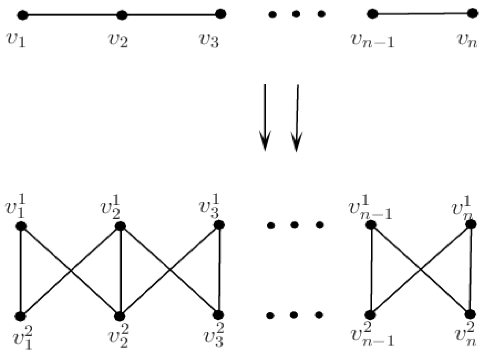
2.2. Isolation Number of the Total Graph

In this section, we describe some bounds on $\iota \left(T\right(G\left)\right)$.

For a graph (G) and a set ($\mathcal{F}$) of graphs, $G_1,G_2,\dots ,G_n$ denote the set of components of G. Let $G_i(i=1,2,\dots ,n)$ denote the component of G. For $i=1,2,\dots ,n$, $\iota (G_i,\mathcal{F})$ denotes the $\mathcal{F}$-isolation number of $G_i$.

Observation 2. 

If G is a graph and $\mathcal{F}$ is a family of graphs, then

$$\iota (G,\mathcal{F})=\sum _{i=1}^n\iota (G_i,\mathcal{F}).$$

Theorem 4. 

Let G be a path ($P_n$); then, $\iota \left(T\left(G\right)\right)=\lceil {\displaystyle \frac{n-1}{3}}\rceil$.

Proof. 

Let $V\left(P_n\right)=\{v_1,v_2,\dots ,v_n\}$; then according to the definition of $T\left(G\right)$, $V\left(T\left(P_n\right)\right)=\{v_1,v_2,\dots ,v_n\}\cup \left\{v_{ij}\right|v_i{v}_j\in E\left(P_n\right)\}$, and $v_{ij}(i\ne 1,n-1;j\ne 2,n)$ is adjacent to $v_i,v_j,v_{(i-1)\left(i\right)}and{v}_{\left(i\right)(i+1)}$. For $i=1,j=2$ and $i=n-1,j=n$, $v_{12}$ is adjacent to $v_1,v_2$ and $v_{23}$, and $v_{(n-1)\left(n\right)}$ is adjacent to $v_{n-1},v_n$ and $v_{(n-2)(n-1)}$. For $n=1or2$, the result is easily proven. Let $n\ge 3$, and if $n\equiv$0 (mod 3), let $S=\left\{v_{ij}\right|i=3k+2,j=i+1\}$ for $k=0,1,2,\dots ,{\displaystyle \frac{n-3}{3}}$. At the moment, $R\left(S\right)=\left\{v_i\right|i=3k+1\}$ for $k=0,1,2,\dots ,{\displaystyle \frac{n-3}{3}}$. According to the structure of $T\left(P_n\right)$, $R\left(S\right)$ is an independent set. Hence, S is an isolating set of $T\left(P_n\right)$; then, $\iota \left(T\left(P_n\right)\right)\le \left|S\right|={\displaystyle \frac{n}{3}}$. On the other hand, let S be an $\iota$ set of $T\left(P_n\right)$. According to the structure of $T\left(P_n\right)$, $\Delta \left(T\left(P_n\right)\right)=4$; then, $4\left|S\right|\ge V\left(T\left(P_n\right)\right)-\left|S\right|\ge 2n-1-\left|S\right|$, that is, $4\iota \left(T\left(P_n\right)\right)\ge 2n-1-\iota \left(T\left(P_n\right)\right)$, $\iota \left(T\left(P_n\right)\right)\ge {\displaystyle \frac{2n-1}{5}}$, as ${\displaystyle \frac{2n-1}{5}}\ge {\displaystyle \frac{n}{3}}$ for $n\ge 3$. Then, $\iota \left(T\left(P_n\right)\right)\ge {\displaystyle \frac{n}{3}}$. Hence, $\iota \left(T\left(P_n\right)\right)={\displaystyle \frac{n}{3}}=\lceil {\displaystyle \frac{n-1}{3}}\rceil$ for $n\equiv$0 (mod 3).

For $n\equiv 1,2\left(mod3\right)$, let $S^{\prime }=\left\{v_{ij}\right|i=3k+2,j=i+1\}\cup \left\{v_n\right\}$ for $k=0,1,2,\dots ,{\displaystyle \frac{n-3}{3}}$. At the moment, $R\left(S^{\prime }\right)=\left\{v_i\right|i=3k+1\}$ for $k=0,1,2,\dots ,{\displaystyle \frac{n-3}{3}}$. According to the structure of $T\left(P_n\right)$, $R\left(S^{\prime }\right)$ is an independent set. Hence, $S^{\prime }$ is an isolating set of $T\left(P_n\right)$; then, $\iota \left(T\left(P_n\right)\right)\le \left|S^{\prime }\right|=\left[{\displaystyle \frac{n}{3}}\right]+1=\lceil {\displaystyle \frac{n}{3}}\rceil$. On the other hand, if $n\equiv$ 1 or 2(mod 3), we prove $\iota \left(T\left(P_n\right)\right)\ge \lceil {\displaystyle \frac{n-1}{3}}\rceil$ by induction on n. For n = 4 or 5, $\iota \left(T\left(P_4\right)\right)=1\ge \lceil {\displaystyle \frac{4-1}{3}}\rceil$ and $\iota \left(T\left(P_5\right)\right)=2\ge \lceil {\displaystyle \frac{5-1}{3}}\rceil$. Therefore, suppose $n>5$ and assume that $\iota \left(T\left(P_{n-1}\right)\right)>\lceil {\displaystyle \frac{n-1-1}{3}}\rceil -1$ is valid for $5<n-1<n$. We now consider the following cases.

Case 1: $n\equiv$1 (mod 3).

In this case, $n-1\equiv$ 0 (mod 3). According to the proof presented above for $n\equiv$0 (mod 3), we have $\iota \left(T\left(P_{n-1}\right)\right)={\displaystyle \frac{n-1}{3}}$. According to the structure of $T\left(P_n\right)$, we have $\iota \left(T\left(P_n\right)\right)=\iota \left(T\left(P_{n-1}\right)\right)$ for $n\equiv$1 (mod 3). Since $n\equiv$1 (mod 3), ${\displaystyle \frac{n-1}{3}}=\lceil {\displaystyle \frac{n-1}{3}}\rceil =\lceil {\displaystyle \frac{n-2}{3}}\rceil$. Hence, according to the above assumption, $\iota \left(T\left(P_n\right)\right)=\iota \left(T\left(P_{n-1}\right)\right)>\lceil {\displaystyle \frac{n-1-1}{3}}\rceil -1=\lceil {\displaystyle \frac{n-2}{3}}\rceil -1=\lceil {\displaystyle \frac{n-1}{3}}\rceil -1$, so $\iota \left(T\left(P_n\right)\right)>\lceil {\displaystyle \frac{n-1}{3}}\rceil -1$, that is, $\iota \left(T\left(P_n\right)\right)\ge \lceil {\displaystyle \frac{n-1}{3}}\rceil$.

Case 2: $n\equiv$2 (mod 3).

In this case, $n-1\equiv$ 1 (mod 3). According to the structure of $T\left(P_n\right)$, we have $\iota \left(T\left(P_n\right)\right)=\iota \left(T\left(P_{n-1}\right)\right)+1$ for $n\equiv$2 (mod 3). Hence, according to the above assumption, $\iota \left(T\left(P_n\right)\right)=\iota \left(T\left(P_{n-1}\right)\right)+1>\lceil {\displaystyle \frac{n-1-1}{3}}\rceil -1+1=\lceil {\displaystyle \frac{n-2}{3}}\rceil >\lceil {\displaystyle \frac{n-4}{3}}\rceil =\lceil {\displaystyle \frac{n-1}{3}}\rceil -1$, so $\iota \left(T\left(P_n\right)\right)>\lceil {\displaystyle \frac{n-1}{3}}\rceil -1$, that is, $\iota \left(T\left(P_n\right)\right)\ge \lceil {\displaystyle \frac{n-1}{3}}\rceil$.

Hence, $\iota \left(T\left(P_n\right)\right)=\lceil {\displaystyle \frac{n-1}{3}}\rceil$ for $n\equiv$1,2 (mod 3).

In conclusion, $\iota \left(T\left(P_n\right)\right)=\lceil {\displaystyle \frac{n-1}{3}}\rceil$. □

Theorem 5. 

Let G be a cycle ($C_n(n\ge 3)$); then, $\iota \left(T\left(G\right)\right)=\lceil {\displaystyle \frac{n}{3}}\rceil$.

Proof. 

Let $V\left(C_n\right)=\{v_1,v_2,\dots ,v_n\}$. According to the definition of $T\left(G\right)$, $V\left(T\left(C_n\right)\right)=\{v_1,v_2,\dots ,v_n\}$ $\cup \left\{v_{ij}\right|v_i{v}_j\in E\left(C_n\right)\}$, and $v_{ij}(i\ne 1,n-1;j\ne 2,n)$ is adjacent to $v_i,v_j,v_{(i-1)\left(i\right)}and{v}_{\left(i\right)(i+1)}$. For $i=1,j=2$ and $i=n-1,j=n$, $v_{12}$ is adjacent to $v_1,v_2$, $v_{23}$ and $v_{1n}$, and $v_{(n-1)\left(n\right)}$ is adjacent to $v_{n-1},v_n$, $v_{(n-2)(n-1)}$ and $v_{1n}$. Let $V_i=\left\{v_i,v_{i+1},v_{i+2},v_{i(i+1)},v_{(i+1)(i+2)},v_{(i+2)(i+3)}\right\}$ and $T_i=T\left(C_n\right)\left[V_i\right]$ be a component of $T\left(C_n\right)$ for $i=3k+1,k=1,2,\dots ,({\displaystyle \frac{n}{3}}-2)$. Let the last component of $T\left(C_n\right)$ be $T_{n-2}=T\left(C_n\right)\left[V_{n-2}\right]$, where $V_{n-2}=\{v_{n-2},v_{n-1},v_n,v_{(n-2)(n-1)},v_{(n-1)\left(n\right)}\}$. Clearly, $\iota \left(T_i\right)=1$ for $i=3k+1,k=1,2,\dots ,({\displaystyle \frac{n}{3}}-1)$. According to $Lemma2.3$, for $k=1,2,\dots ,({\displaystyle \frac{n}{3}}-2)$, $\iota \left(T\left(C_n\right)\right)={\displaystyle \sum _{i=1}^{3k+1}}\iota \left(T_i\right)+\iota \left(T_{n-2}\right)={\displaystyle \frac{2n-6}{6}}+1={\displaystyle \frac{n}{3}}$. Since $\iota \left(T\left(C_n\right)\right)$ is an integer, $\iota \left(T\left(C_n\right)\right)=\lceil {\displaystyle \frac{n}{3}}\rceil$ for $n\equiv 1,2\left(mod3\right)$. Hence, $\iota \left(T\left(C_n\right)\right)=\lceil {\displaystyle \frac{n}{3}}\rceil$ for $n\ge 3$. □

Corollary 1. 

The following statements hold.

(i) 

$\iota \left(T\left(S_n\right)\right)=1.$

(ii) 

$\iota \left(T\left(K_n\right)\right)=\lfloor {\displaystyle \frac{n}{2}}\rfloor .$

(iii) 

$\iota \left(T\left(K_{k_1,k_2,\dots ,k_n}\right)\right)=\iota \left(T\left(K(m,n)\right)\right)=2.$

Theorem 6. 

Let G be a connected graph on n vertices and m edges with a maximum degree of Δ; then,

(i) 

$\iota \left(T\left(G\right)\right)\ge \iota \left(G\right)\ge {\displaystyle \frac{m}{{\Delta }^2}}.$

(ii) 

$\iota \left(T\left(G\right)\right)\le {\displaystyle \frac{n-2\Delta +1}{2}}.$

Proof. 

(i) Let $G=(V,E)$; then, according to the definition of $T\left(G\right)$, let $T\left(G\right)=(V\cup E,E^{\prime })$ and $S^{\prime }$ be a minimum isolating set of $T\left(G\right)$. Let $S^{\prime }=A\cup B=\left\{v_{ij}\right|v_i{v}_j\in E\left(G\right)and{v}_{ij}\in S^{\prime }for1\le i,j\le n\}\cup \left\{v_k\right|v_k\in V\left(G\right)and{v}_k\in S^{\prime }for1\le k\le n\}$. Let $H=\{v_i,v_k|v_{ij}\in S^{\prime },v_k\in S^{\prime }for1\le i,j,k\le n\}$; then, $\left|H\right|=|S^{\prime }|$. Clearly, $R_G\left(H\right)$ is an independent set of G. Hence, H is an isolating set of G. Then, $\iota \left(G\right)\le \left|H\right|=|S^{\prime }|=\iota \left(T\left(G\right)\right)$. For the right-hand inequality, we start with the edge bound of G to prove it. Let S be a minimum isolating set of G. Since G has a maximum degree of $\Delta$, $E(S,N(S\left)\right)\le \Delta \left|S\right|$. On the other hand, the vertices of $N\left(S\right)$ have at least one neighbor in S, so we have $E\left(N\right(S),V\setminus S)\le (\Delta -1)\left|N\right(S\left)\right|\le (\Delta -1)\Delta \left|S\right|$, that is, $E\left(G\right)\le \Delta \left|S\right|+(\Delta -1)\Delta \left|S\right|={\Delta }^2\left|S\right|={\Delta }^2\iota \left(G\right)$. Hence, $\iota \left(G\right)\ge {\displaystyle \frac{m}{{\Delta }^2}}$. In conclusion, we have $\iota \left(T\left(G\right)\right)\ge \iota \left(G\right)\ge {\displaystyle \frac{m}{{\Delta }^2}}.$

$\left(ii\right)$ Let G be a graph with n vertices and m edges and a maximum degree of $\Delta$. According to the definition of $T\left(G\right)$, we have $V\left(T\right(G\left)\right)=m+n$ and $\Delta \left(T\right(G\left)\right)=2\Delta$. Let v be the vertex of $T\left(G\right)$ with a maximum degree of $2\Delta$ and $V\left(T{\left(G\right)}^{*}\right)=V\left(T\left(G\right)\right)-N_{T\left(G\right)}\left[v\right]$. Let I be the independent set of $T{\left(G\right)}^{*}$ and $H=T{\left(G\right)}^{*}-I$. For the dominating set (D) of H, we have $\left|D\right|\le {\displaystyle \frac{V\left(T{\left(G\right)}^{*}\right)-\left|I\right|}{2}}\le {\displaystyle \frac{V\left(T{\left(G\right)}^{*}\right)}{2}}={\displaystyle \frac{m+n-2\Delta -1}{2}}$. Clearly, $D\cup \left\{v\right\}$ is an isolating set of $T\left(G\right)$; then, $\iota \left(T\left(G\right)\right)\le \left|D\right|+1\le {\displaystyle \frac{m+n-2\Delta +1}{2}}$. □

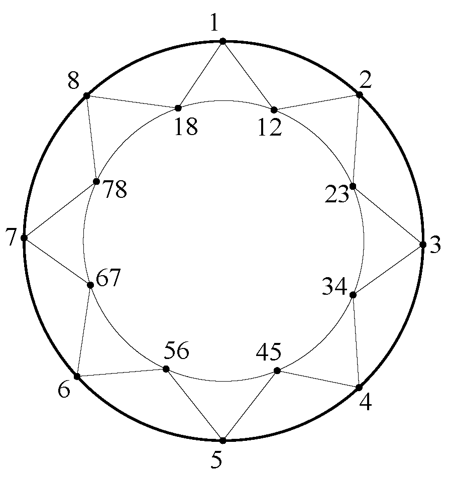
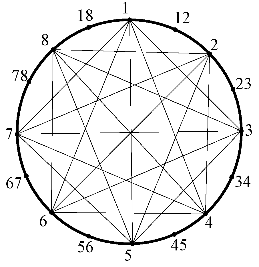
2.3. Isolation Number of Central Graph

In this section, we describe some bounds on $\iota \left(C\right(G\left)\right)$.

Theorem 7. 

For a complete bipartite graph ($K_{m,n}$) that is not $K_{1,1}$, $\iota \left(C\left(K_{m,n}\right)\right)=2$.

Proof. 

Let $V\left(K_{m,n}\right)=\{v_1^1,v_2^1,\dots ,v_m^1\}\cup \{v_1^2,v_2^2,\dots ,v_n^2\}$ and $E\left(K_{m,n}\right)=\left\{v_i^1{v}_j^2\right|1\le i\le m,1\le j\le n\}$. According to the definition of $C\left(G\right)$, $V\left(C\left(K_{m,n}\right)\right)=V\left(K_{m,n}\right)\cup \left\{v_{ij}\right|v_i^1{v}_j^2\in E\left(K_{m,n}\right)\}$. For any two vertices ($v_i^1(1\le i\le m)$ and $v_j^2(1\le j\le n)$) from $V\left(C\left(K_{m,n}\right)\right)$, and let $S=\{v_i^1,v_j^2\}$. Since $v_i^1$ is adjacent to $v_j^1(1\le j\le mandj\ne i)$ and $v_j^2$ is adjacent to $v_j^2(1\le i\le nandi\ne j)$, $R\left(S\right)=V\left(C\left(K_{m,n}\right)\right)\setminus N_{C\left(K_{m,n}\right)}\left[S\right]$. Hence, we have S is an isolating set of $C\left(K_{m,n}\right)$. Thus, $\iota \left(C\left(K_{m,n}\right)\right)\le 2$. In addition, we have $\iota \left(C\left(K_{m,n}\right)\right)\ge 1$.

Now, we show $\iota (C\left(K_{m,n}\right)\ne 1$. Let S be an isolating set of $C\left(K_{m,n}\right)$ and $\left|S\right|=1$. If $S\subseteq V\left(K_{m,n}\right)$, then $S=\left\{v_i^1\right\}$ or $\left\{v_j^2\right\}$. Without loss of generality, assume that $S=\left\{v_i^1\right\}$. Then, there exist edges $v_i^1{v}_l^2(1\le j,l\le n)$ and edges $v_j^2{v}_{ij}(1\le i\le m,1\le j\le n)$ in $R\left(S\right)$. Thus, S is not an isolating set of $C\left(K_{m,n}\right)$. If $S\subseteq \left\{v_{ij}\right|v_i^1{v}_j^2\in E\left(K_{m,n}\right),1\le i\le m,1\le j\le n\}$, clearly, $R\left(S\right)$ is not an independent set; then, S is not an isolating of $C\left(K_{m,n}\right)$, si $\iota \left(C\left(K_{m,n}\right)\right)>1$. Hence, $\iota \left(C\left(K_{m,n}\right)\right)=2$. □

Theorem 8. 

Let G be a connected graph with n vertices and m edges; then, ${\iota }_1\left(C\left(G\right)\right)\le {\displaystyle \frac{m+3}{3}}$.

Proof. 

Let G be a graph with n vertices and m edges. According to the definition of $C\left(G\right)$, the maximum degree ($\Delta$) of $C\left(G\right)$ is $n-1$. Assume that v is a vertex with a maximum degree of $\Delta$ in $C\left(G\right)$ and $C{\left(G\right)}^{*}=C\left(G\right)-N_{C\left(G\right)}\left[v\right]$. Let $X\subseteq V\left(C{\left(G\right)}^{*}\right)$ be the set of vertices of all components of, at most, two vertices in $C{\left(G\right)}^{*}$, and let Y be the set of vertices of all $C_5$ components of $C{\left(G\right)}^{*}$ and H be a minimum $\left\{K_{1,2}\right\}$-isolating set of $C\left(G\right)\left[Y\right]$. Clearly, we have $\left|H\right|={\displaystyle \frac{\left|Y\right|}{5}}$. Let S be a minimum isolating set of $C{\left(G\right)}^{*}-(X\cup Y)$. In particular, if $V\left(C{\left(G\right)}^{*}\right)-(X\cup Y)=Ø$, we say $S=Ø$. It is obvious that $\left\{v\right\}\cup H\cup S$ is a $\left\{K_{1,2}\right\}$-isolating set of $C\left(G\right)$. According to Theorem 2.3, we have $\left|S\right|\le {\displaystyle \frac{V\left(C{\left(G\right)}^{*}\right)-\left|X\right|-\left|Y\right|}{3}}$. Hence,

$$\begin{array}{cc}\hfill {\iota }_1\left(C\left(G\right)\right)& \le 1+\left|X\right|+\left|Y\right|\hfill \\ \hfill & \le 1+{\displaystyle \frac{\left|Y\right|}{5}}+{\displaystyle \frac{V\left(C{\left(G\right)}^{*}\right)-\left|X\right|-\left|Y\right|}{3}}\hfill \\ \hfill & \le 1+{\displaystyle \frac{\left|Y\right|}{3}}+{\displaystyle \frac{V\left(C{\left(G\right)}^{*}\right)-\left|Y\right|}{3}}\hfill \\ \hfill & =1+{\displaystyle \frac{|V\left(C\left(G\right)\right)-N_{C\left(G\right)}\left[v\right]|}{3}}\hfill \\ \hfill & =1+{\displaystyle \frac{n+m-(n-1)-1}{3}}\hfill \\ \hfill & ={\displaystyle \frac{m+3}{3}}\hfill \end{array}$$

(1)

□

3. Conclusions

In this paper, we introduced the concepts of partial domination–isolation in graphs and researched the isolation numbers of several classes of transformed graphs. The main contents include an upper bound on the isolation number of the B(G) graph of a connected graph, upper and lower bounds on the isolation number of the total graph of a connected graph with respect to the maximum degree of the graph and an upper bound on the $K_{1,2}$-isolation number of the center graph of a connected graph with respect to the number of edges.

For the isolation number of several types of transition graphs studied in this paper, here are some issues that can be further studied and discussed:

Question 1: What isolation numbers of transition graphs can also be studied in graph theory?

Question 2: What is the relationship between the isolation number and $\mathcal{F}$-isolation number of various conversion graphs and other parameters of the original graph?

References

1. Berge, C. Theory of Graphs and Its Applications; Dunod: Paris, France, 1958. [Google Scholar]
2. Hansberg, A.; Meierling, D.; Volkmann, L. A general method in the theory of domination in graphs. Int. J. Comput. Math. 2010, 87, 2915–2924. [Google Scholar] [CrossRef]
3. Haynes, T.; Hedetniemi, S.; Slater, P. Fundamentals of Domination in Graphs; CRC Press: New York, NY, USA, 1998. [Google Scholar]
4. West, D. Introduction to Graph Theory; Longman: London, UK, 1985. [Google Scholar]
5. Hao, G.S.; Lim, M.H.; Ong, Y.S.; Huang, H.; Wang, G.G. Domination landscape in evolutionary algorithms and its applications. Soft Comput. 2019, 23, 3563–3570. [Google Scholar] [CrossRef]
6. Stephen, S.; Rajan, B.; Ryan, J.; Grigorious, C.; William, A. Power domination in certain chemical structures. J. Discret. Algorithms 2015, 33, 10–18. [Google Scholar] [CrossRef]
7. Rajan, R.S.; Anitha, J.; Rajasingh, I. 2-Power Domination in Certain Interconnection Networks. Procedia Comput. Sci. 2015, 57, 738–744. [Google Scholar] [CrossRef]
8. Corcoran, P.; Gagarin, A. Heuristics for k-domination models of facility location problems in street networks. Comput. Oper. Res. 2021, 133, 53–68. [Google Scholar] [CrossRef]
9. Zhu, X.; Yu, J.; Lee, W. New dominating sets in social networks. J. Glob. Optim. 2010, 48, 633–642. [Google Scholar] [CrossRef]
10. Caroa, Y.; Hansbergb, A. Partial domination-the isolation number of a graph. Filomath 2017, 31, 3925–3944. [Google Scholar] [CrossRef]
11. Favaron, O.; Kaemawichanurat, P. Inequalities between the Kk-isolation number and the independent Kk-isolation number of a graph. Discret. Appl. Math. 2021, 289, 93–97. [Google Scholar] [CrossRef]
12. Peter, B.; Kurt, F.; Pawaton, K. Isolation of k-cliques. Discret. Math. 2020, 343, 111879. [Google Scholar]
13. Shin-ichi, T.; Thiradet, J.; Pawaton, K. Isolation number of maximal outerplanar graphs. Discret. Appl. Math. 2019, 267, 215–218. [Google Scholar]
14. Zhang, G.; Wu, B. K1,2-isolation in graphs. Discret. Appl. Math. 2021, 304, 365–374. [Google Scholar] [CrossRef]
15. Magdalena, L.; María José, S.; Adriana, D.; Francisco, J.V. Isolation Number versus Domination number of trees. Mathematics 2021, 9, 1325. [Google Scholar] [CrossRef]
16. Peter, B. Isolation of Cycles. Graphs Comb. 2020, 36, 631–637. [Google Scholar]
17. Peter, B. Isolation of connected graphs. Discret. Appl. Math. 2023, 339, 154–165. [Google Scholar]
18. Chen, J.; Xu, S. P5-isolation in graphs. Discret. Appl. Math. 2023, 340, 331–349. [Google Scholar] [CrossRef]
19. Zhang, G.; Wu, B. A note on the Cycle Isolation Number of Graphs. Bull. Malays. Math. Sci. Soc. 2024, 47, 57. [Google Scholar] [CrossRef]
20. Zhang, G.; Wu, B. Cycle Isolation of Graphs with Small Girth. Graphs Comb. 2024, 40, 38. [Google Scholar] [CrossRef]
21. Yang, Z.; Arockiaraj, M.; Prabhu, S.; Arulperumjothi, M.; Liu, J.N. Second Zagreb and Sigma Indices of Semi and TotalTransformations of Graphs. Complexity 2021, 2021, 6828424. [Google Scholar] [CrossRef]
22. Kalpana, M.; Vijayalakshmi, D. On b-coloring of central graph of some graphs. Commun. Fac. Sci. Univ. Ank. Ser. A1 Math. Stat. 2019, 68, 1229–1239. [Google Scholar] [CrossRef]
23. Peter, B.; Kurt, F.; Pawaton, K. Isolation of k-cliques II. Discret. Appl. Math. 2022, 345, 112641. [Google Scholar]
Figure 1. The bipartite graph ( B ( P n ) ).
Mathematics 13 00116 g001
Figure 2. The total graph ( T ( C 8 ) ).
Mathematics 13 00116 g002
Figure 3. The central graph ( C ( C 8 ) ).
Mathematics 13 00116 g003
Figure 4. A BFS tree of the Petersen graph.
Mathematics 13 00116 g004
Disclaimer/Publisher’s Note: The statements, opinions and data contained in all publications are solely those of the individual author(s) and contributor(s) and not of MDPI and/or the editor(s). MDPI and/or the editor(s) disclaim responsibility for any injury to people or property resulting from any ideas, methods, instructions or products referred to in the content.