Analysis of High-Order Bright–Dark Rogue Waves in (2+1)-D Variable-Coefficient Zakharov Equation via Self-Similar and Darboux Transformations

Abstract

This paper conducts an in-depth study on the self-similar transformation, Darboux transformation, and the excitation and propagation characteristics of high-order bright–dark rogue wave solutions in the (2+1)-dimensional variable-coefficient Zakharov equation. The Zakharov equation is instrumental for studying complex nonlinear interactions in these areas, with specific implications for energy transfer processes in plasma and nonlinear wave propagation systems. By analyzing bright–dark rogue wave solutions—phenomena that are critical in understanding high-energy events in optical and fluid environments—this research elucidates the intricate dynamics of energy concentration and dissipation. Using the self-similar transformation method, we map the (2+1)-dimensional equation to a more tractable (1+1)-dimensional nonlinear Schrödinger equation form. Through the Lax pair and Darboux transformation, we successfully construct high-order solutions that reveal how variable coefficients influence rogue wave features, such as shape, amplitude, and dynamics. Numerical simulations demonstrate the evolution of these rogue waves, offering novel perspectives for predicting and mitigating extreme wave events in engineering applications.This paper crucially advances the practical understanding and manipulation of nonlinear wave phenomena in variable environments, providing significant insights for applications in optical fibers, atmospheric physics, and marine engineering.

1. Introduction

The Zakharov equation is a significant mathematical model in plasma physics, employed for studying nonlinear phenomena, particularly the nonlinear propagation and interaction of waves. Its applicability extends beyond plasma research to encompass the comprehension of complex nonlinear phenomena such as wave formation in oceans and the propagation of light waves in optical fibers [1]. A comprehensive analysis of the Zakharov equation unveils the mechanisms of nonlinear wave interactions and explores various wave patterns formed under specific conditions, such as solitons and rogue waves [2]. In 1972, the renowned physicist and mathematician V.E. Zakharov proposed this system of equations coupling electric field and particle perturbations while investigating the interaction between plasma and lasers. This system combines the nonlinear Schrödinger equation with a wave equation containing strong nonlinear terms, forming what is known as the Zakharov equation. Zakharov successfully computed soliton wave solutions of this system of equations, providing profound explanations for physical phenomena such as the deep density cavities observed in laser–target interactions, garnering widespread attention in the international physics community [3]. To date, the Zakharov equation is considered one of the most comprehensive models for describing the coupling of low-frequency and high-frequency waves in nonlinear systems [4], particularly in plasma physics, where the high-frequency mode describes electron-acoustic waves and the low-frequency mode describes ion-acoustic waves. For instance, Langmuir wave turbulence in plasmas with large temperature ratios is often described by this equation [5].

Due to its potent application potential in theoretical physics, oceanography, optics, and quantum fluid dynamics, the Zakharov equation has attracted extensive research efforts from physicists and mathematicians. These efforts have led to numerous innovative and influential findings. For example, regarding the (2+1)-dimensional Zakharov equation [6]:

$$i{u}_t+u_{xy}+uv=0,v_x={\left|u\right|}_y^2$$

When $x=y$, the above equation reduces to the well-known (1+1)-dimensional nonlinear Schrödinger (NLS) equation; when $t=0$, it simplifies to the complex sine-Gordon equation.

Radha and others investigated the (2+1)-dimensional Zakharov equation and demonstrated its Painlevé property. Through an in-depth analysis of singular structures, they further showcased the richness and complexity of this equation in describing nonlinear phenomena. Particularly, their derivation of a bilinear form provided new analytical methods and insights for subsequent researchers [7]. Strachan utilized the bilinear method to construct a new method for inducing localized coherent structures by freely selecting arbitrary functions. This method not only broadened the application scope of the Zakharov equation but also provided a new approach for understanding and controlling coherent structures in nonlinear systems [8]. Chen and others, building upon the bilinear method, obtained breather solutions and first-order rogue wave solutions. They also utilized the Sato operator theory to derive first- and higher-order rogue wave solutions, depicting the dynamic evolution of nonlinear waves under specific conditions [9]. Wang and others combined the bilinear method with the long-wave limit approach to obtain rational and mixed solutions for solitons, enriching the forms of solutions to the Zakharov equation [10]. Yin and others employed the Jacobi elliptic function expansion method to solve the equation for traveling wave solutions and solitary wave solutions, effectively revealing the propagation characteristics of traveling waves and solitary waves in nonlinear systems [11]. Guo and others, inspired by the traveling wave solutions, utilized the homogeneous balance principle and the structure of a class of nonlinear ordinary differential equation solutions to investigate the richer exact solution expressions of the equation using an extended (G′/G) expansion method, providing more effective means for controlling nonlinear wave dynamics [12]. He adopted the ($\Phi /\Psi$) expansion method to obtain rich hyperbolic cotangent function solutions and, by selecting appropriate parameters, vividly depicted the propagation of waves [13]. Hua and others utilized the generalized algebraic method to derive many new exact solutions, including rational function solutions, Jacobi elliptic function solutions, mixed elliptic function solutions, knotted solutions, singular solutions, and trigonometric function solutions [14]. The acquisition of these solutions not only enriched our understanding of the Zakharov equation but also revealed the propagation and evolution characteristics of nonlinear waves in various forms.

Previous researchers have extensively explored the (2+1)-dimensional Zakharov equation on multiple levels, uncovering its important mathematical properties and providing powerful mathematical tools and theoretical support for understanding and controlling nonlinear wave dynamics. In this paper, to expand the application of the Zakharov equation in the study of nonlinear systems, we will seek bright–dark rogue wave solutions of the (2+1)-dimensional variable-coefficient Zakharov equation, aiming to achieve new breakthroughs in the study of nonlinear systems. The following sections introduce the concepts related to bright–dark rogue wave solutions and the methods for solving the equation.

Rogue wave solutions, also known as bright rogue wave solutions, are a special class of solutions in the study of nonlinear partial differential equations and have been a hot topic in nonlinear science in recent years. They have been observed in many natural and laboratory systems [15,16,17,18,19], especially in fluid dynamics and nonlinear optics describing wave phenomena [20,21]. The concept of rogue waves originated in the ocean to describe a peculiar type of ocean wave, characterized as a sudden wave that significantly increases in amplitude over a short time against a background of zero or relatively small amplitude, greatly exceeding the average level, and then disappearing shortly thereafter, showing a very localized nature. In optics, bright rogue waves can be seen as high-intensity light pulses that appear suddenly against an almost completely dark background and then rapidly disappear. This phenomenon has been observed in nonlinear optical fiber transmission, ocean wave dynamics, and other areas, often associated with the analytical solutions of basic nonlinear models such as the nonlinear Schrödinger equation (NLSE) and the Zakharov equation. Dark rogue wave solutions [22,23,24,25,26,27], also known as rogue hole solutions [28], represent another phenomenon relative to bright rogue waves. They form a localized low-intensity region or ‘hole’ in a continuous wave background. These rogue wave solutions appear as dark areas against a relatively bright background and then disappear within a short time [29]. The study of bright and dark rogue waves reveals the complex dynamics of energy concentration and dissipation that can occur in nonlinear systems under certain conditions [30,31,32].

Self-similar transformation plays a significant role in the study of nonlinear evolution equations [33]. It is a scaling transformation based on the fundamental mathematical concept of self-similarity, which refers to an object or mathematical entity exhibiting similar forms or structures at different scales. In nonlinear dynamical systems in physics and mathematics, self-similar transformation often translates the solution of an equation from one scale to another while preserving the form of the solution in order to find analytical or approximate solutions under specific conditions. This means that if a solution, after appropriate scaling, can satisfy the same equation again, then this solution is considered self-similar. By applying self-similar transformations, we can simplify a complex nonlinear problem into a more manageable form, or reduce a multi-parameter problem to one with fewer parameters, thereby making it easier to find analytical or approximate solutions [34].

The Darboux transformation, originally developed by Gaston Darboux, is an instrumental method in the study of nonlinear evolution equations, particularly in the construction of explicit solutions, such as rogue wave solutions. This transformation operates through an elegant algebraic procedure that enables the generation of new solutions from known ones without solving the differential equations directly. Its application in the field of integrable systems, such as the nonlinear Schrödinger equation (NLS) and the Korteweg-de Vries (KdV) equation, has been pivotal in deepening our understanding of the dynamics of rogue waves. These solutions, often characterized by their extreme, transient nature, provide crucial insights into phenomena ranging from oceanography to optics. The Darboux transformation not only facilitates the exploration of these complex wave structures but also significantly simplifies the process of obtaining higher-order rogue wave solutions. For instance, studies by Matveev and Salle demonstrated the transformation’s robustness in generating multi-soliton solutions, a foundational aspect for analyzing rogue waves [35]. Further, Guo et al. expanded this application to uncover dynamics of rogue waves in fiber optics using the NLS model [36]. These applications underscore the transformation’s utility in translating theoretical mathematical concepts into practical analytical tools that can predict and analyze high-energy wave phenomena in various physical contexts [37,38,39,40].

Within the realm of nonlinear dynamics, the self-similar and Darboux transformations stand out for their unique abilities to streamline complex problem-solving. The self-similar transformation reduces the complexity of nonlinear equations, converts multi-parameter problems into simpler forms, and maintains the structural integrity of solutions across varying scales. This characteristic is invaluable in modeling phenomena with inherent self-similarity, such as turbulent flows and fractal patterns in nature. Conversely, the Darboux transformation excels in generating exact solutions from known ones, a process pivotal for revealing intricate dynamics like rogue waves. It also adeptly handles variable-coefficient equations, making it a potent tool in theoretical and applied sciences where conditions often vary, highlighting its practical significance in adapting models to real-world scenarios. These transformations not only provide clearer insights into the mathematical structures they address but also enhance the applicability of solutions to physical and engineering problems.

This paper, based on the research method provided in the literature [10], first establishes the self-similar transformation of the variable-coefficient (2+1)-dimensional Zakharov equation. After reducing it to the (1+1)-dimensional variable-coefficient NLS equation, with the aid of its Lax pair and Darboux transformation, we obtain the excitation of higher-order bright and dark rogue waves on the x-y plane. Furthermore, we conduct a study on various parameters and perform a dynamics analysis of the propagation characteristics of bright and dark rogue waves. Then, we will analyze the propagation characteristics of bright and dark rogue waves and draw plenty of pictures, from which we will show the relationship between rogue wave characteristics and system parameters, and the evolution process of rogue waves under the influence of multiple factors. This paper, has for the first time successfully constructed high-order bright–dark rogue wave solutions in the (2+1)-dimensional variable-coefficient Zakharov equation through the self-similar transformation and the Darboux transformation.

2. Self-Similar Transformation of the (2+1)-Dimensional Variable-Coefficient Zakharov Equation

This is the (2+1)-dimensional variable-coefficient Zakharov equation:

$$\begin{array}{c}\hfill a_1\left(t\right)i{u}_t+a_2\left(t\right)u_{xy}+a_3\left(t\right)uv=0,v_x={\left|u\right|}_y^2.\end{array}$$

(1)

Within the restraint of the Equation (1), the function u(x, y, t) is a complex-valued function representing the wave function. This function depends on two spatial dimensions (x and y) and time (t), evolving dynamically according to the equation. It is important to note that u(x, y, t) being complex-valued, encodes both the amplitude and phase of the wave, providing a rich mathematical framework for describing various wave phenomena in (2+1) dimensions.

Introducing the self-similar transformation:

$$\begin{array}{cc}\hfill & u(x,y,t)={\rho }_1\left(t\right)\varphi (\xi ,\zeta )exp\left[i\phi (x,y,t)\right]\hfill \end{array}$$

(2)

$$\begin{array}{cc}\hfill & v(x,y,t)={\rho }_2\left(t\right)\psi (\xi ,\zeta )\hfill \end{array}$$

(3)

where ${\rho }_1\left(t\right)$, ${\rho }_2\left(t\right)$, $\varphi (\xi ,\zeta )$, $\psi (\xi ,\zeta )$, $\phi (x,y,t)$, and $\xi =\xi (x,y,t)$, $\zeta =\zeta \left(t\right)$ are the to-be-determined functions of the specified variables, substitution yields:

$$\begin{array}{cc}\hfill u_t& =e^{i\phi (x,y,t)}\varphi {\rho }_{1t}+e^{i\phi (x,y,t)}{\rho }_1\left({\zeta }_t{\varphi }_{\zeta }+{\xi }_t{\varphi }_{\xi }\right)+i{e}^{i\phi (x,y,t)}\varphi {\rho }_1\left(t\right){\phi }_t,\hfill \end{array}$$

(4)

$$\begin{array}{cc}\hfill u_{xy}& =e^{i\phi (x,y,t)}{\xi }_{xy}{\rho }_1\left(t\right){\varphi }^{(1,0)}[\xi (x,y,t),\zeta \left(t\right)]\hfill \\ \hfill & +e^{i\phi (x,y,t)}{\xi }_x{\xi }_y{\rho }_1\left(t\right){\varphi }^{(2,0)}[\xi (x,y,t),\zeta \left(t\right)]\hfill \\ \hfill & +i{e}^{i\phi (x,y,t)}{\xi }_x{\rho }_1\left(t\right){\varphi }^{(1,0)}[\xi (x,y,t),\zeta \left(t\right)]{\phi }_y\hfill \\ \hfill & +i{e}^{i\phi (x,y,t)}{\xi }_y{\rho }_1\left(t\right){\varphi }^{(1,0)}[\xi (x,y,t),\zeta \left(t\right)]{\phi }_x\hfill \\ \hfill & -e^{i\phi (x,y,t)}\varphi [\xi (x,y,t),\zeta \left(t\right)]{\rho }_1\left(t\right){\phi }_y{\phi }_x\hfill \\ \hfill & +i{e}^{i\phi (x,y,t)}\varphi [\xi (x,y,t),\zeta \left(t\right)]{\rho }_1\left(t\right){\phi }_{xy},\hfill \end{array}$$

(5)

$$v_x={\xi }_x{\rho }_2\left(t\right){\psi }^{(1,0)}[\xi (x,y,t),\zeta \left(t\right)],$$

(6)

$$\begin{array}{cc}\hfill {\left|u\right|}_y^2& =2e^{-2\mathrm{Im}\left[\phi \right(x,y,t\left)\right]}\left|\varphi [\xi (x,y,t),\zeta \left(t\right)]{\rho }_1\left(t\right)\right|{\xi }_y{\rho }_1\left(t\right)\frac{d}{dt}\left|\varphi [\xi (x,y,t),\zeta \left(t\right)]{\rho }_1\left(t\right)\right|\hfill \\ \hfill & \times {\varphi }^{(1,0)}[\xi (x,y,t),\zeta \left(t\right)]\hfill \\ \hfill & -2e^{-2\mathrm{Im}\left[\phi \right(x,y,t\left)\right]}{\left|\varphi [\xi (x,y,t),\zeta \left(t\right)]{\rho }_1\left(t\right)\right|}^2\frac{d}{dt}\mathrm{Im}\left[\phi (x,y,t)\right]{\phi }_y\hfill \\ \hfill & =e^{i\phi (x,y,t)}\varphi [\xi (x,y,t),\zeta \left(t\right)]{\rho }_{1t}\hfill \\ \hfill & +e^{i\phi (x,y,t)}{\rho }_1\left(t\right)\left({\zeta }_t{\varphi }^{(0,1)}[\xi (x,y,t),\zeta \left(t\right)]+{\xi }_t{\varphi }^{(1,0)}[\xi (x,y,t),\zeta \left(t\right)]\right)\hfill \\ \hfill & +i{e}^{i\phi (x,y,t)}\varphi [\xi (x,y,t),\zeta \left(t\right)]{\rho }_1\left(t\right){\phi }_t(x,y,t).\hfill \end{array}$$

(7)

After substituting into the original equation, it leads to the derivation:

$$\begin{array}{cc}\hfill i\varphi & \left(a_1{\rho }_{1t}+a_2{\rho }_1{\phi }_{xy}\right)+a_2{\rho }_1{\xi }_{xy}{\varphi }_{\xi }+i{\varphi }_{\xi }{\rho }_1\left(a_2{\phi }_x{\xi }_y+a_1{\xi }_t+a_2{\phi }_y{\xi }_x\right)\hfill \\ \hfill & -{\rho }_1\varphi \left(a_1{\phi }_t+a_2{\phi }_x{\phi }_y\right)+i{\rho }_1{\zeta }_t{\varphi }_{\zeta }{a}_1+{\rho }_1{\xi }_x{\xi }_y{\varphi }_{\xi \xi }{a}_2+{\rho }_1{\rho }_2\varphi \psi a_3=0\hfill \end{array}$$

(8)

$$\begin{array}{c}\hfill {\rho }_2{\psi }_{\xi }{\xi }_x={\rho }_1^2{\left|\varphi \right|}_{\xi }^2{\xi }_y\end{array}$$

(9)

In order to transform into the (1+1)-dimensional variable-coefficient nonlinear

Schrödinger (NLS) equation, the variables above need to satisfy the following relationships:

$$\begin{array}{cc}\hfill & {\xi }_{xy}=0\hfill \end{array}$$

(10)

$$\begin{array}{cc}\hfill & a_1{\xi }_t+a_2{\phi }_x{\xi }_y+a_2{\phi }_y{\xi }_x=0\hfill \end{array}$$

(11)

$$\begin{array}{cc}\hfill & a_1{\phi }_t+a_2{\phi }_x{\phi }_y=0\hfill \end{array}$$

(12)

$$\begin{array}{cc}\hfill & {\zeta }_t={\xi }_x{\xi }_y\hfill \end{array}$$

(13)

$$\begin{array}{cc}\hfill & a_1{\rho }_{1t}+a_2{\rho }_1{\phi }_{xy}=0\hfill \end{array}$$

(14)

$$\begin{array}{cc}\hfill & {\rho }_1^2{\xi }_y={\rho }_2{\xi }_x=2{\xi }_x{\zeta }_t\hfill \end{array}$$

(15)

After satisfying the above relationships, the original equation has been transformed into the (1+1)-dimensional variable-coefficient nonlinear Schrödinger (NLS) equation:

$$\begin{array}{c}\hfill i{a}_1\left(t\right){\varphi }_{\zeta }+a_2\left(t\right){\varphi }_{\xi \xi }+a_3\left(t\right)2\varphi {\left|\varphi \right|}^2=0\end{array}$$

(16)

Given the certain symmetry of the Zakharov equation with respect to the spatial variables x and y, and in conjunction with the literature, we define the similarity variable $\xi$ as:

$$\begin{array}{c}\hfill \xi =\kappa \left(t\right)(x+\gamma y)+\omega \left(t\right)\end{array}$$

(17)

Combining Equation (17), and from Equation (11), we can obtain:

$$\begin{array}{c}\hfill \phi (x,y,t)=-\frac{\alpha \left(t\right)}{2}{(x+\gamma y)}^2-\beta \left(t\right)(x+\gamma y)-\sigma \left(t\right)\end{array}$$

(18)

From Equations (11)–(15), we sequentially obtain:

$$\begin{array}{cc}\hfill F\left(t\right)& ={\int }_1^t\frac{2\gamma \mathrm{a}2\left(k_1\right)}{\mathrm{a}1\left(k_1\right)}d{k}_1\hfill \\ \hfill \alpha \left(t\right)& =-\frac{1}{F\left(t\right)+c_1}\hfill \\ \hfill \kappa \left(t\right)& =\frac{c_1{c}_2}{c_1+F\left(t\right)}\hfill \\ \hfill \beta \left(t\right)& =\frac{c_3{c}_4}{c_3+F\left(t\right)}\hfill \\ \hfill \omega \left(t\right)& =c_1{c}_2{c}_{4}ln(c_1+F\left(t\right))-ln\left(c_1\right)\hfill \\ \hfill \sigma \left(t\right)& =\frac{-c_3^2{c}_4^2}{c_3+F\left(t\right)}+c_4^2+c_5\hfill \\ \hfill \zeta \left(t\right)& =\gamma c_1^2{c}_2^2{\int }_1^t\frac{1}{{(c_1+F\left(k_4\right))}^2}d{k}_4+c_3\hfill \\ \hfill {\rho }_1\left(t\right)& =\frac{\sqrt{2}{C}_1{C}_2}{C_1+F\left(t\right)}\hfill \\ \hfill {\rho }_2\left(t\right)& =\frac{2\gamma c_1^2{c}_2^2}{{(c_1+F\left(t\right))}^2}\hfill \end{array}$$

(19)

We have now successfully used the self-similar transformation to map the (2+1)-dimensional variable-coefficient Zakharov equation to the (1+1)-dimensional variable-coefficient nonlinear Schrödinger (NLS) equation.

3. The Lax Pair and Darboux Transformation of the (1+1)-Dimensional Variable-Coefficient Nonlinear Schrödinger (NLS) Equation

For our equation:

$$\begin{array}{c}\hfill i{a}_1\left(t\right){\varphi }_{\zeta }+a_2\left(t\right){\varphi }_{\xi \xi }+a_3\left(t\right)2\varphi {\left|\varphi \right|}^2=0\end{array}$$

(20)

Its Lax pair is: [41]

$$\begin{array}{c}\hfill {\Psi }_{\xi }=U\Psi \end{array}$$

(21)

$$\begin{array}{c}\hfill U=\left(\begin{array}{cc}\lambda a_1\left(t\right)& a_1\left(t\right)\varphi \\ -a_1\left(t\right)\overline{\varphi }& -\lambda a_1\left(t\right)\end{array}\right)\end{array}$$

(22)

and

$$\begin{array}{c}\hfill {\Psi }_{\zeta }=V\Psi \end{array}$$

(23)

$$\begin{array}{c}\hfill V=i\left(\begin{array}{cc}2a_1\left(t\right)a_2\left(t\right){\lambda }^2+\frac{a_3\left(t\right)}{a_1\left(t\right)}{\left|\varphi \right|}^2& a_2\left(t\right){\varphi }_{\xi }+2a_1\left(t\right)a_2\left(t\right)\lambda \varphi \\ a_2\left(t\right)\overline{{\varphi }_{\xi }}-2a_1\left(t\right)a_2\left(t\right)\lambda \overline{\varphi }& -2a_1\left(t\right)a_2\left(t\right){\lambda }^2-\frac{a_3\left(t\right)}{a_1\left(t\right)}{\left|\varphi \right|}^2\end{array}\right)\end{array}$$

(24)

Substituting into the Lax equation $U_{\zeta }-V_{\xi }+[U,V]=0$, to satisfy the compatibility condition, it is required that

$$\begin{array}{c}\hfill a_1\left(t\right)a_2\left(t\right)=\frac{a_3\left(t\right)}{a_1\left(t\right)}\end{array}$$

(25)

This indicates that among the three variable coefficients of the original equation, only two degrees of freedom exist.

In the (1+1)-dimensional variable-coefficient nonlinear Schrödinger (NLS) equation, the Darboux transformation is defined as follows:

$$\begin{array}{c}\hfill \Psi \left[1\right]=T\left[1\right]\Psi ,\varphi \left[1\right]=\varphi +2({\lambda }_1^{*}-{\lambda }_1){\left(P\left[1\right]\right)}_{21}\end{array}$$

(26)

where

$$\begin{array}{c}\hfill T\left[1\right]=\lambda -{\lambda }_1^{*}+({\lambda }_1^{*}-{\lambda }_1)P\left[1\right],P\left[1\right]=\frac{{\Psi }_1{\Psi }_1^{†}}{{\Psi }_1^{†}{\Psi }_1}\end{array}$$

(27)

${\Psi }_1$ is a particular solution of the linear system (21)–(24) when substituting $\lambda ={\lambda }_1$; ${\left(P\left[1\right]\right)}_{21}$ represents the element in the second row and the first column of the matrix $P\left[1\right]$, and the dagger symbol denotes the conjugate transpose of the matrix.

If we substitute N distinct seed solutions ${\Psi }_k,(k=1,2,\cdots ,N)$ into the Lax pair, then we can repeatedly perform the fundamental Darboux transformation. To carry out the second transformation, we substitute ${\Psi }_2$, which is given by ${\Psi }_2{\left[1\right]=T\left[1\right]|}_{\lambda ={\lambda }_2}{\Psi }_2$, therefore:

$$\begin{array}{c}\hfill T\left[2\right]=\lambda -{\lambda }_2^{*}+({\lambda }_2^{*}-{\lambda }_2)P\left[2\right],P\left[2\right]=\frac{{\Psi }_2\left[1\right]{\Psi }_2^{†}\left[1\right]}{{\Psi }_2^{†}\left[1\right]{\Psi }_2\left[1\right]}\end{array}$$

(28)

Let ${\Psi }_1\left({\lambda }_1\right),{\Psi }_2\left({\lambda }_2\right),\cdots ,{\Psi }_n\left({\lambda }_n\right)$ be n independent solutions of the Lax pair. We perform a Taylor expansion for each of them at ${\lambda }_i$, yielding:

${\Psi }_i({\lambda }_i+\delta )={\Psi }_i+{\Psi }_i^{\left[1\right]}\delta +{\Psi }_i^{\left[2\right]}{\delta }^2+\cdots +{\Psi }_i^{\left[m_i\right]}{\delta }^N+\cdots$$(i=1,2,\cdots ,n)$ where

$$\begin{array}{c}\hfill {\Psi }_i^{\left[j\right]}=\frac{1}{j!}\frac{{\partial }^j}{\partial {\zeta }^j}{\Psi }_i{\left(\zeta \right)|}_{\zeta ={\zeta }_i}(j=1,2,\cdots )\end{array}$$

(29)

We define:

$$\begin{array}{c}\hfill T={\Gamma }_n{\Gamma }_{n-1}\cdots {\Gamma }_1{\Gamma }_0{\Gamma }_i=T_i\left[m_i\right]\cdots T_i\left[1\right](i\ge 1){\Gamma }_0=I\end{array}$$

(30)

where [36]

$$\begin{array}{c}\hfill T_i\left[j\right]=\lambda -{\lambda }_i^{*}+({\lambda }_i^{*}-{\lambda }_i)P_i\left[j\right]P_i\left[j\right]=\frac{{\Psi }_i[j-1]{\Psi }_i^{†}[j-1]}{{\Psi }_i^{†}[j-1]{\Psi }_i[j-1]}1\le j\le m_i\end{array}$$

(31)

$$\begin{array}{c}\hfill {\Psi }_i\left[0\right]=({\Gamma }_{i-1}\cdots {\Gamma }_1{\Gamma }_0){|}_{\lambda ={\lambda }_i}{\Psi }_i\end{array}$$

(32)

$$\begin{array}{cc}\hfill {\Psi }_i\left[k\right]& =\underset{\delta \to 0}{lim}\frac{[\delta +T_i{\left[k\right]}_{\lambda ={\lambda }_i}]\cdots [\lambda +T_i{\left[2\right]}_{\lambda ={\lambda }_i}][\delta +T_i{\left[1\right]}_{\lambda ={\lambda }_i}]{\Gamma }_{i-1}({\lambda }_i+\delta )\cdots {\Gamma }_1({\lambda }_i+\delta ){\Gamma }_0{\Psi }_i({\lambda }_i+\delta )}{{\delta }^k}\hfill \end{array}$$

(33)

$$\begin{array}{cc}\hfill & ={\Psi }_i+\sum _{s=1}^k\sum _{\begin{array}{c}{m}_i\ge h_1^{\left(i\right)}>\cdots >h_{k_i}^{\left(i\right)}\ge 1\\ i\ge g_1>\cdots >g_l\ge 1\\ if{g}_1=i,then{h}_1^{\left(1\right)}\le k\end{array}}^{{\sum }_{j=1}^l{k}_j+s=k}(T_{g_1}\left[h_1^{\left(1\right)}\right]\cdots T_{g_1}\left[h_{k_1}^{\left(1\right)}\right]\cdots T_{g_1}\left[h_1^{\left(l\right)}\right]\cdots T_{g_l}\left[h_{k_l}^{\left(l\right)}\right]){|}_{\lambda ={\lambda }_1}{\Psi }_i^{\left[s\right]}\hfill \end{array}$$

(34)

where $1\le k\le m_i$, we thus obtain the general Darboux transformation of the nonlinear Schrödinger (NLS) equation:

$$\begin{array}{c}\hfill \Psi \left[N\right]=T\Psi \varphi \left[N\right]=\varphi +2\sum _{i=1}^n\sum _{j=1}^{m_i}({\lambda }_i^{*}-{\lambda }_i){\left(P_i\left[m_j\right]\right)}_{21}\left(N=n+\sum _{k=1}^n{m}_k\right)\end{array}$$

(35)

Now, let us start from the seed solution $\varphi \left[0\right]=e^{i\zeta \int 2a_1\left(t\right)a_2\left(t\right)dt}$ and set $\lambda =ih$.

We obtain

$$\begin{array}{c}\hfill {\Psi }_1\left(h\right)=\left(\begin{array}{c}i(c_1{e}^{\Omega }-c_2{e}^{-\Omega })e^{-i\zeta \int a_1\left(t\right)a_2\left(t\right)dt}\\ (c_2{e}^{\Omega }-c_1{e}^{-\Omega })e^{i\zeta \int a_1\left(t\right)a_2\left(t\right)dt}\end{array}\right)\end{array}$$

(36)

where,

$$\begin{array}{cc}\hfill c_1& =\frac{\sqrt{h-\sqrt{h^2-1}}}{\sqrt{h^2-1}}\hfill \end{array}$$

(37)

$$\begin{array}{cc}\hfill c_2& =\frac{\sqrt{\sqrt{h^2-1}+h}}{\sqrt{h^2-1}}\hfill \end{array}$$

(38)

$$\begin{array}{cc}\hfill \Omega & =\sqrt{h^2-1}(\xi +ih\zeta \int 2a_1\left(t\right)a_2\left(t\right)dt-\int \frac{a_2\left(t\right)}{a_1\left(t\right)}dt)\hfill \end{array}$$

(39)

Let $h=1+d^2$, expanding the vector function ${\Psi }_1\left(d\right)$ at d = 0, we have

$${\Psi }_1\left(d\right)={\Psi }_1\left(0\right)+{\Psi }_1^{\left[1\right]}{d}^2+\cdots$$

$${\Psi }_1\left(0\right)=\left(\begin{array}{c}i{e}^{-i\zeta \int \mathrm{a}1\left(t\right)\mathrm{a}2\left(t\right)dt}\left(4i\zeta \int \mathrm{a}1\left(t\right)\mathrm{a}2\left(t\right)dt-2\int \frac{\mathrm{a}2\left(t\right)}{\mathrm{a}1\left(t\right)}dt+2\xi -1\right)\\ e^{i\zeta \int \mathrm{a}1\left(t\right)\mathrm{a}2\left(t\right)dt}\left(4i\zeta \int \mathrm{a}1\left(t\right)\mathrm{a}2\left(t\right)dt-2\int \frac{\mathrm{a}2\left(t\right)}{\mathrm{a}1\left(t\right)}dt+2\xi +1\right)\end{array}\right),$$

and

$${\Psi }_1^{\left[1\right]}=\left(\begin{array}{c}{\Delta }_a^{11}\\ {\Delta }_b^{11}\end{array}\right),$$

where

$$\begin{array}{cc}\hfill {\Delta }_a^{11}& =\frac{1}{12}{e}^{-i\zeta \int \mathrm{a}1\left(t\right)\mathrm{a}2\left(t\right)dt}\left(12i{\left(\int \frac{\mathrm{a}2\left(t\right)}{\mathrm{a}1\left(t\right)}dt\right)}^2(4i\zeta \int \mathrm{a}1\left(t\right)\mathrm{a}2\left(t\right)dt+2\xi -1)-6i\int \frac{\mathrm{a}2\left(t\right)}{\mathrm{a}1\left(t\right)}dt{(4i\zeta \int \mathrm{a}1\left(t\right)\mathrm{a}2\left(t\right)dt+2\xi -1)}^2\right.\hfill \\ & +4\zeta (\int \mathrm{a}1\left(t\right)\mathrm{a}2\left(t\right)dt)(-3(4(\xi -1)\xi +5)+4\zeta (\int \mathrm{a}1\left(t\right)\mathrm{a}2\left(t\right)dt)(4\zeta \int \mathrm{a}1\left(t\right)\mathrm{a}2\left(t\right)dt-6i\xi +3i))-8i{\left(\int \frac{\mathrm{a}2\left(t\right)}{\mathrm{a}1\left(t\right)}dt\right)}^3\hfill \\ & \left.+i\left(2\xi \left(4{\xi }^2-6\xi +3\right)+3\right)\right)\hfill \end{array}$$

$$\begin{array}{cc}\hfill {\Delta }_b^{11}& =\frac{1}{12}{e}^{i\zeta \int \mathrm{a}1\left(t\right)\mathrm{a}2\left(t\right)dt}\left(12{\left(\int \frac{\mathrm{a}2\left(t\right)}{\mathrm{a}1\left(t\right)}dt\right)}^2(4i\zeta \int \mathrm{a}1\left(t\right)\mathrm{a}2\left(t\right)dt+2\xi +1)-6\int \frac{\mathrm{a}2\left(t\right)}{\mathrm{a}1\left(t\right)}dt{(4i\zeta \int \mathrm{a}1\left(t\right)\mathrm{a}2\left(t\right)dt+2\xi +1)}^2\right.\hfill \\ \hfill & +4\zeta (\int \mathrm{a}1\left(t\right)\mathrm{a}2\left(t\right)dt)(4\zeta (\int \mathrm{a}1\left(t\right)\mathrm{a}2\left(t\right)dt)(-4i\zeta \int \mathrm{a}1\left(t\right)\mathrm{a}2\left(t\right)dt-6\xi -3)+3i(4\xi (\xi +1)+5))-8{\left(\int \frac{\mathrm{a}2\left(t\right)}{\mathrm{a}1\left(t\right)}dt\right)}^3\hfill \\ \hfill & +2\xi (4{\xi }^2+6\xi +3)-3)\hfill \end{array}$$

and

$${\Psi }_1^{\left[2\right]}=\left(\begin{array}{c}{\Delta }_a^{12}\\ {\Delta }_b^{12}\end{array}\right)$$

where

$$\begin{array}{cc}\hfill {\Delta }_a^{12}& =\frac{1}{480}i{e}^{-i\zeta \int \mathrm{a}1\left(t\right)\mathrm{a}2\left(t\right)dt}\left(2\left(512i{\zeta }^5{\left(\int \mathrm{a}1\left(t\right)\mathrm{a}2\left(t\right)dt\right)}^5+640{\zeta }^4{\left(\int \mathrm{a}1\left(t\right)\mathrm{a}2\left(t\right)dt\right)}^4\left(-2\int \frac{\mathrm{a}2\left(t\right)}{\mathrm{a}1\left(t\right)}dt+2\xi -1\right)\right.\right.\hfill \\ \hfill & -320i{\zeta }^3{\left(\int \mathrm{a}1\left(t\right)\mathrm{a}2\left(t\right)dt\right)}^3\left(4{\left(\int \frac{\mathrm{a}2\left(t\right)}{\mathrm{a}1\left(t\right)}dt\right)}^2-8\xi \int \frac{\mathrm{a}2\left(t\right)}{\mathrm{a}1\left(t\right)}dt+4(\xi -1)\xi +15\right)\hfill \\ \hfill & +80{\zeta }^2{\left(\int \mathrm{a}1\left(t\right)\mathrm{a}2\left(t\right)dt\right)}^2\left(4{\left(\int \frac{\mathrm{a}2\left(t\right)}{\mathrm{a}1\left(t\right)}dt\right)}^3-12\xi {\left(\int \frac{\mathrm{a}2\left(t\right)}{\mathrm{a}1\left(t\right)}dt\right)}^2+\left(12(\xi -1)\xi +33\right)\int \frac{\mathrm{a}2\left(t\right)}{\mathrm{a}1\left(t\right)}dt\right.\hfill \\ \hfill & \left.-2\xi \left(4{\xi }^2-6\xi +33\right)+27\right)+80i\zeta \int \mathrm{a}1\left(t\right)\mathrm{a}2\left(t\right)dt\left({\left(\int \frac{\mathrm{a}2\left(t\right)}{\mathrm{a}1\left(t\right)}dt\right)}^3-3\xi {\left(\int \frac{\mathrm{a}2\left(t\right)}{\mathrm{a}1\left(t\right)}dt\right)}^2\right.\hfill \\ \hfill & +\left(6{\xi }^2-8\xi +21\right)\int \frac{\mathrm{a}2\left(t\right)}{\mathrm{a}1\left(t\right)}dt\hfill \\ \hfill & \left.+\xi (-2(\xi -2)\xi -21)+15\right)+\left(\int \frac{\mathrm{a}2\left(t\right)}{\mathrm{a}1\left(t\right)}dt\right)\left(20\left(2\xi \left(4{\xi }^2-6\xi +9\right)-3\right)\int \frac{\mathrm{a}2\left(t\right)}{\mathrm{a}1\left(t\right)}dt\right.\hfill \\ \hfill & +8{\left(\int \frac{\mathrm{a}2\left(t\right)}{\mathrm{a}1\left(t\right)}dt\right)}^2\left(\int \frac{\mathrm{a}2\left(t\right)}{\mathrm{a}1\left(t\right)}dt\left(-2\int \frac{\mathrm{a}2\left(t\right)}{\mathrm{a}1\left(t\right)}dt+10\xi -5\right)-5(4(\xi -1)\xi +3)\right)\hfill \\ \hfill & \left.\left.-40\xi \left(\xi \right(2(\xi -2)\xi +9)-3)+15\right)+420i\zeta \int \mathrm{a}1\left(t\right)\mathrm{a}2\left(t\right)dt+2\xi \left(4\xi \left(2\xi \left(\xi \right(2\xi -5)+15)-15\right)-15\right)-45\right)\hfill \end{array}$$

$$\begin{array}{cc}\hfill {\Delta }_b^{12}& =\frac{1}{480}{e}^{i\zeta \int \mathrm{a}1(t)\mathrm{a}2(t)dt}\left(40{\left(\int \frac{\mathrm{a}2(t)}{\mathrm{a}1(t)}dt\right)}^2\left(4\zeta \left(\int \mathrm{a}1(t)\mathrm{a}2(t)dt\right)\left(4\zeta \left(\int \mathrm{a}1(t)\mathrm{a}2(t)dt\right)\left(-4i\zeta \int \mathrm{a}1(t)\mathrm{a}2(t)dt-6\xi -3\right)\right.\right.\right.\hfill \\ \hfill & \left.\left.+3i\left(4\xi (\xi +1)+7\right)\right)+2\xi \left(4{\xi }^2+6\xi +9\right)+3\right)+10\int \frac{\mathrm{a}2\left(t\right)}{\mathrm{a}1\left(t\right)}dt\left(-\left(2\xi +1\right)\left(2\xi \left(4{\xi }^2+6\xi +15\right)-3\right)\right.\hfill \\ \hfill & +16\zeta \left(\int \mathrm{a}1(t)\mathrm{a}2(t)dt\right)\left(2\zeta \left(\int \mathrm{a}1(t)\mathrm{a}2(t)dt\right)\left(8\zeta \left(\int \mathrm{a}1(t)\mathrm{a}2(t)dt\right)\left(-\zeta \int \mathrm{a}1(t)\mathrm{a}2(t)dt+2i\xi +i\right)\right.\right.\hfill \\ \hfill & \left(\left.\left.+12\xi (\xi +1)+33\right)-i\left(2\xi \left(4{\xi }^2+6\xi +21\right)+15\right)\right)\right)+4\zeta \left(\int \mathrm{a}1(t)\mathrm{a}2(t)dt\right)\left(8\zeta \left(\int \mathrm{a}1(t)\mathrm{a}2(t)dt\right)\right.\hfill \\ \hfill & \left(-5\left(2\xi \left(4{\xi }^2+6\xi +33\right)+27\right)+4\zeta \left(\int \mathrm{a}1(t)\mathrm{a}2(t)dt\right)\left(2\zeta \left(\int \mathrm{a}1(t)\mathrm{a}2(t)dt\right)\left(4i\zeta \int \mathrm{a}1(t)\mathrm{a}2(t)dt+10\xi +5\right)\right.\right.\hfill \\ \hfill & \left.\left.-5i\left(4\xi (\xi +1)+15\right)\right)+5i\left(2\xi +1\right)\left(2\xi \left(4{\xi }^2+6\xi +39\right)+21\right)\right)+80{\left(\int \frac{\mathrm{a}2\left(t\right)}{\mathrm{a}1\left(t\right)}dt\right)}^4\left(4i\zeta \int \mathrm{a}1(t)\mathrm{a}2(t)dt+2\xi +1\right)\hfill \\ \hfill & -80{\left(\int \frac{\mathrm{a}2(t)}{\mathrm{a}1(t)}dt\right)}^3\left(8\zeta \left(\int \mathrm{a}1(t)\mathrm{a}2(t)dt\right)\left(-2\zeta \int \mathrm{a}1(t)\mathrm{a}2(t)dt+2i\xi +i\right)+4\xi (\xi +1)+3\right)\hfill \\ \hfill & \left.-32{\left(\int \frac{\mathrm{a}2(t)}{\mathrm{a}1(t)}dt\right)}^5+2\xi \left(4\xi \left(2\xi \left(\xi \left(2\xi +5\right)+15\right)+15\right)-15\right)+45\right)\hfill \end{array}$$

It is clear that ${\Psi }_1\left(0\right)$ is a solution for the Lax pair at $\lambda =i$. We take ${\lambda }_k=i(k=1,2,3,\cdots )$

Utilizing Equations (30)–(35), we specifically substitute to obtain:

$${\Psi }_1\left[1\right]=\underset{d\to 0}{lim}\frac{[i{d}^2+T_1\left[1\right]]{\Psi }_1\left(d\right)}{d^2}=T_1\left[1\right]{\Psi }_1^{\left[1\right]}+{\Psi }_1\left(0\right)$$

$$T_1\left[1\right]=2i(I-\frac{{\Psi }_1\left(0\right){\Psi }_1{\left(0\right)}^{†}}{{\Psi }_1{\left(0\right)}^{†}{\Psi }_1\left(0\right)})$$

Substituting into Formula (26), we obtain

$$\begin{array}{c}\hfill \varphi \left[1\right]=e^{2i\zeta \int \mathrm{a}1\left(t\right)\mathrm{a}2\left(t\right)dt}(1+\frac{D_1}{D_2})\end{array}$$

(40)

where

$$\begin{array}{cc}\hfill D_1& =-(32+16i){\zeta }^2{(\int \mathrm{a}1\left(t\right)\mathrm{a}2\left(t\right)dt)}^2\hfill \\ \hfill & -8\zeta \int \mathrm{a}1\left(t\right)\mathrm{a}2\left(t\right)dt+(16+8i)\xi \left(\int \frac{\mathrm{a}2\left(t\right)}{\mathrm{a}1\left(t\right)}dt\right)-(8+4i){\left(\int \frac{\mathrm{a}2\left(t\right)}{\mathrm{a}1\left(t\right)}dt\right)}^2-\left((8+4i){\xi }^2\right)+(-2+i)\hfill \end{array}$$

$$\begin{array}{c}\hfill D_2=2\left(16{\zeta }^2{(\int \mathrm{a}1\left(t\right)\mathrm{a}2\left(t\right)dt)}^2-8\xi \left(\int \frac{\mathrm{a}2\left(t\right)}{\mathrm{a}1\left(t\right)}dt\right)+4{\left(\int \frac{\mathrm{a}2\left(t\right)}{\mathrm{a}1\left(t\right)}dt\right)}^2+4{\xi }^2+1\right)\end{array}$$

meanwhile

$T_1\left[2\right]=\lambda -{\lambda }_1^{*}+({\lambda }_1^{*}-{\lambda }_1)P_1\left[2\right]$

Substituting into Equation (28), we obtain the second-order rogue wave solution.

$$\varphi \left[2\right]=e^{2i\zeta \int \mathrm{a}1\left(t\right)\mathrm{a}2\left(t\right)dt}(1+\frac{D_3}{D_4})$$

The specific analysis results for $D_3$ and $D_4$ are detailed in Appendix A.

Upon specific substitution into Equations (30)–(35), the corresponding Darboux transformation for the third-order rogue wave solution is:

$$T_1\left[3\right]=\lambda -{\lambda }_2^{*}+({\lambda }_2^{*}-{\lambda }_2)P_1\left[3\right]$$

$$P_1\left[3\right]=\frac{{\Psi }_1\left[2\right]{\Psi }_1{\left[2\right]}^{†}}{{\Psi }_1{\left[2\right]}^{†}{\Psi }_1\left[2\right]}$$

$$\varphi \left[3\right]=\varphi \left[2\right]+2({\lambda }_2^{*}-{\lambda }_2){\left(P_1\left[3\right]\right)}_{21}$$

The obtained third-order rogue wave solution is detailed in Appendix B.

When $a_i\left(t\right)=1$ (where $i=1,2,3$), the results for the anomalous waves coincide with the constant coefficient results found in [42].

Assuming that N distinct solutions ${\Psi }_i={({\psi }_i,{\upsilon }_i)}^T$$(i=1,2,\cdots ,N)$ are given for the spectral problem (21)–(24) at $\lambda ={\lambda }_1=\cdots ={\lambda }_n$ and expanding

$$\begin{array}{cc}\hfill & {\left({\lambda }_i+\delta \right)}^j{\psi }_i\left({\lambda }_i+\delta \right)={\lambda }_i^j{\psi }_i+{\psi }_i[j,1]\delta +{\psi }_i[j,2]{\delta }^2+\cdots +{\psi }_i\left[j,m_i\right]{\delta }^{m_i}+\cdots \hfill \end{array}$$

(41)

$$\begin{array}{cc}\hfill & {\left({\lambda }_i+\delta \right)}^j{\upsilon }_i\left({\lambda }_i+\delta \right)={\lambda }_i^j{\upsilon }_i+{\upsilon }_i[j,1]\delta +{\upsilon }_i[j,2]{\delta }^2+\cdots +{\upsilon }_i\left[j,m_i\right]{\delta }^{m_i}+\cdots \hfill \end{array}$$

(42)

with [43]

$${\psi }_i[j,m]={\left.\frac{1}{m!}\frac{{\partial }^m}{\partial {\lambda }^m}\left[{\lambda }^j{\psi }_i\left(\lambda \right)\right]\right|}_{\lambda ={\lambda }_i},{\upsilon }_i[j,m]={\left.\frac{1}{m!}\frac{{\partial }^m}{\partial {\lambda }^m}\left[{\lambda }^j{\upsilon }_i\left(\lambda \right)\right]\right|}_{\lambda ={\lambda }_i}$$

$(j=0,1,\dots ,N,m=1,2,3,\dots )$

Based on the N-fold Darboux transformation (29)–(35) for the variable coefficient NLS Equation (20), when substituting the seed solution

$$\begin{array}{c}\hfill \varphi \left[0\right]=\varphi =e^{i\zeta \int 2a_1\left(t\right)a_2\left(t\right)dt},\end{array}$$

(43)

we have

$$\begin{array}{c}\hfill \varphi \left[N\right]=\varphi -2\frac{D_a}{D_b},D_a=det\left([H_1\cdots H_n]\right),D_b=det\left([G_1\cdots G_n]\right)\end{array}$$

(44)

where $N=n+{\sum }_{k=1}^n{m}_k$ and [42]

$$\begin{array}{cc}\hfill & G_i=\left[\begin{array}{cccccc}{\lambda }_i^{N-1}{\psi }_i& \cdots & {\psi }_i\left[N-1,m_i\right]& -{\lambda }_i^{*(N-1)}{\upsilon }_i^{*}& \cdots & -{\upsilon }_i{\left[N-1,m_i\right]}^{*}\\ \cdots & \cdots & \cdots & \cdots & \cdots & \cdots \\ {\psi }_i& \cdots & {\psi }_i\left[0,m_i\right]& -{\upsilon }_i^{*}& \cdots & -{\upsilon }_i{\left[0,m_i\right]}^{*}\\ {\lambda }_i^{N-1}{\upsilon }_i& \cdots & {\upsilon }_i\left[N-1,m_i\right]& {\lambda }_i^{*(N-1)}{\psi }_i^{*}& \cdots & {\psi }_i{\left[N-1,m_i\right]}^{*}\\ \cdots & \cdots & \cdots & \dots & \cdots & \\ {\upsilon }_i& \cdots & {\upsilon }_i\left[0,m_i\right]& {\psi }_i^{*}& \cdots & {\psi }_i{\left[0,m_i\right]}^{*}\end{array}\right],\hfill \end{array}$$

(45)

$$\begin{array}{cc}\hfill & H_i=\left[\begin{array}{cccccc}{\lambda }_i^N{\upsilon }_i& \cdots & {\upsilon }_i\left[N,m_i\right]& {\lambda }_i^{*N}{\psi }_i^{*}& \cdots & {\psi }_i{\left[N,m_i\right]}^{*}\\ {\lambda }_i^{N-2}{\psi }_i& \cdots & {\psi }_i\left[N-2,m_i\right]& -{\lambda }_i^{*(N-2)}{\upsilon }_i^{*}& \cdots & -{\upsilon }_i{\left[N-2,m_i\right]}^{*}\\ \cdots & \cdots & \cdots & \cdots & \cdots & \\ {\psi }_i& \cdots & {\psi }_i\left[0,m_i\right]& -{\upsilon }_i^{*}& \cdots & -{\upsilon }_i{\left[0,m_i\right]}^{*}\\ {\lambda }_i^{N-1}{\upsilon }_i& \cdots & {\upsilon }_i\left[N-1,m_i\right]& {\lambda }_i^{*(N-1)}{\psi }_i^{*}& \cdots & {\psi }_i{\left[N-1,m_i\right]}^{*}\\ \cdots & \cdots & \cdots & \cdots & \cdots & \\ {\upsilon }_i& \cdots & {\upsilon }_i\left[0,m_i\right]& {\psi }_i^{*}& \cdots & {\psi }_i{\left[0,m_i\right]}^{*}\end{array}\right].\hfill \end{array}$$

(46)

We point out that, applied to special seed solution (43), (39) enables us to have a determinant form for higher-order rogue wave solutions. We considered $({\psi }_1,{\upsilon }_1)$ above at (36)–(39).

Substituting ${\lambda }_k=i(k=1,2,3,\cdots )$, the associated Taylor expansions become

$$\begin{array}{cc}\hfill i^j{\left(1+h^2\right)}^j{\psi }_1\left(h\right)& =i^j{\psi }_1\left(0\right)+{\psi }_1[j,1]h^2+\cdots +{\psi }_1[j,N]h^{2N}+\cdots ,\hfill \\ \hfill {\psi }_1[j,n]& ={\left.\frac{1}{\left(2n\right)!}\frac{{\partial }^{2n}}{\partial h^{2n}}\left[i^j{\left(1+h^2\right)}^j{\psi }_1\left(d\right)\right]\right|}_{h=0},\hfill \\ \hfill i^j{\left(1+h^2\right)}^j{\upsilon }_1\left(h\right)& =i^j{\upsilon }_1\left(0\right)+{\upsilon }_1[j,1]h^2+\cdots +{\upsilon }_1[j,N]h^{2N}+\cdots ,\hfill \\ \hfill {\upsilon }_1[j,n]& ={\left.\frac{1}{\left(2n\right)!}\frac{{\partial }^{2n}}{\partial h^{2n}}\left[i^j{\left(1+h^2\right)}^j{\upsilon }_1\left(h\right)\right]\right|}_{h=0}\hfill \end{array}$$

$(j=0,1,\dots ,N,n=1,2,3,\dots )$

Then it follows that the N th-order rogue wave solution for the NLS Equation (20), reads

$$\begin{array}{c}\hfill \varphi \left[N\right]=\left[1-2\frac{D_a}{D_b}\right]e^{2i\zeta \int \mathrm{a}1\left(t\right)\mathrm{a}2\left(t\right)dt}\end{array}$$

(47)

where

$$\begin{array}{cc}& D_a=\left|\begin{array}{cccccc}{i}^{N-1}{\psi }_1& \cdots & {\psi }_1[N-1,N-1]& -{(-i)}^{(N-1)}{\upsilon }_1^{*}& \cdots & -{\upsilon }_1{[N-1,N-1]}^{*}\\ \cdots & \cdots & \cdots & \cdots & \cdots & \cdots \\ {\psi }_1& \cdots & {\psi }_1[0,N-1]& -{\upsilon }_1^{*}& \cdots & -{\upsilon }_1{[0,N-1]}^{*}\\ i^{N-1}{\upsilon }_1& \cdots & {\upsilon }_1[N-1,N-1]& -i^{(N-1)}{\psi }_1^{*}& \cdots & {\psi }_1{[N-1,N-1]}^{*}\\ \cdots & \cdots & \cdots & \cdots & \cdots & \\ {\upsilon }_1& \cdots & {\upsilon }_1[0,N-1]& {\psi }_1^{*}& \cdots & {\psi }_1{[0,N-1]}^{*}\end{array}\right|\hfill \\ & D_b=\left|\begin{array}{cccccc}{i}^N{\upsilon }_1& \cdots & {\upsilon }_1[N,N-1]& {(-i)}^N{\psi }_1^{*}& \cdots & {\psi }_1{[N,N-1]}^{*}\\ i^{N-2}{\psi }_1& \cdots & {\psi }_1[N-2,N-1]& -{(-i)}^{(N-2)}{\upsilon }_1^{*}& \cdots & -{\upsilon }_1{[N-2,N-1]}^{*}\\ \cdots & \cdots & \dots & \dots & \cdots & \\ {\psi }_1& \cdots & {\psi }_1[0,N-1]& -{\upsilon }_1^{*}& \cdots & -{\upsilon }_1{[0,N-1]}^{*}\\ i^{N-1}{\upsilon }_1& \cdots & {\upsilon }_1[N-1,N-1]& {(-i)}^{(N-1)}{\psi }_1^{*}& \cdots & {\psi }_1{[N-1,N-1]}^{*}\\ \dots & \cdots & \dots & \dots & \cdots & \\ {\upsilon }_1& \cdots & {\upsilon }_1[0,N-1]& {\psi }_1^{*}& \cdots & {\psi }_1{[0,N-1]}^{*}\end{array}\right|.\hfill \end{array}$$

Utilizing the self-similar inverse transformation, as derived through Equations (2) and (3), the results for higher-order rogue wave solutions (47) of the (1+1)-D variable-coefficient NLS equation, can be substituted back into the original Equation (1). Consequently, we obtain the N-th order rogue wave solution for the original equation as follows:

$$u(x,y,t)\left[N\right]=\frac{\sqrt{2}{C}_1{C}_2}{C_1+F\left(t\right)}\varphi \left[N\right]exp[i(\frac{{(x+\gamma y)}^2}{2(F\left(t\right)+C_1)}-\frac{c_3{c}_4(x+\gamma y)}{c_3+F\left(t\right)}+\frac{c_3^2{c}_4^2}{c_3+F\left(t\right)}-c_4^2-c_5)]$$

When $a_i\left(t\right)=1$ (where $i=1,2$), the results for the anomalous waves $u\left[1\right]$ and $u\left[2\right]$ coincide with the constant coefficient results found in the literature [10].

4. Dynamics Analysis of the Propagation Characteristics of Bright and Dark Rogue Waves

The constant $c_5$ does not appear in the modulus part of the rogue wave solution, hence, it does not affect the amplitude of the rogue wave. Because the constant parameters $c_i$ ($i=1,2,3,4$) and $\gamma$ are mutually independent of the time-dependent coefficients, we initially choose the set of time-dependent coefficients $a_2\left(t\right)=2$ and $a_1\left(t\right)=1$ to investigate the influence of constant parameters and time on the rogue wave. The parameter for $F\left(t\right)$ is automatically determined once $a_1\left(t\right)$, $a_2\left(t\right)$, and $\gamma$ are specified, given that $F\left(t\right)$ is defined by (19), the integral expression $F\left(t\right)={\int }_1^t\frac{2\gamma a_2\left(k_1\right)}{a_1\left(k_1\right)}d{k}_1$.

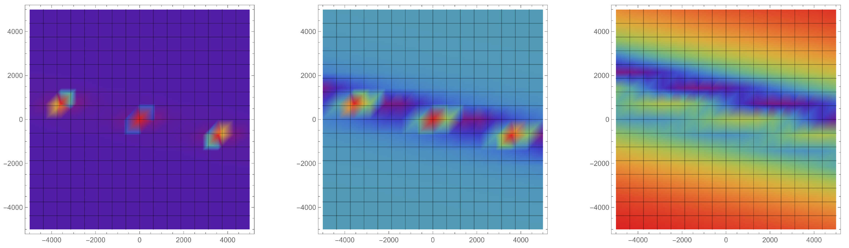
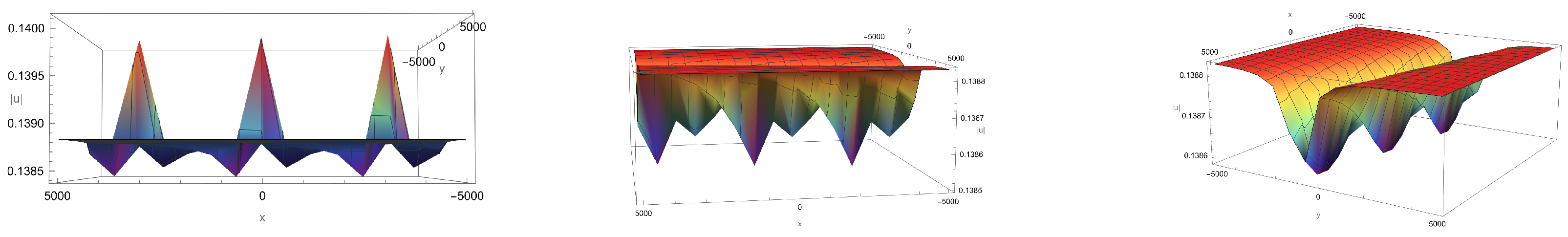
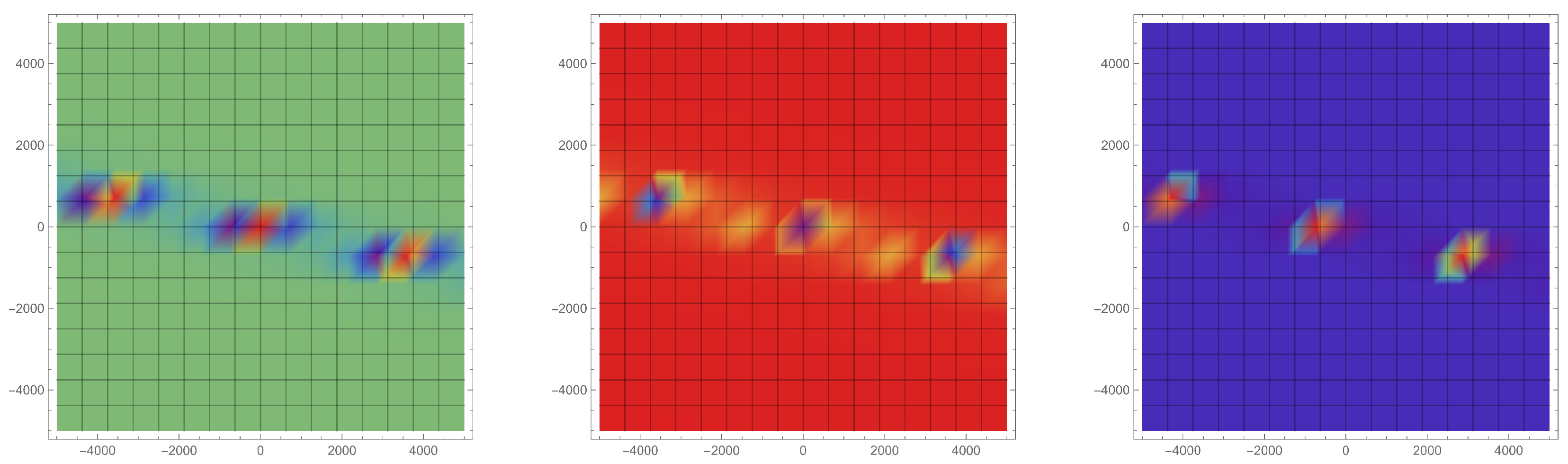
Figure 1 and its corresponding density plot in Figure 2 illustrate the initial state and evolution of first-order bright–dark rogue waves. The three-dimensional plot and the density plot reveal a concentrated wave energy core that diffuses over time while maintaining a clear distinction between the bright and dark components of the wave.

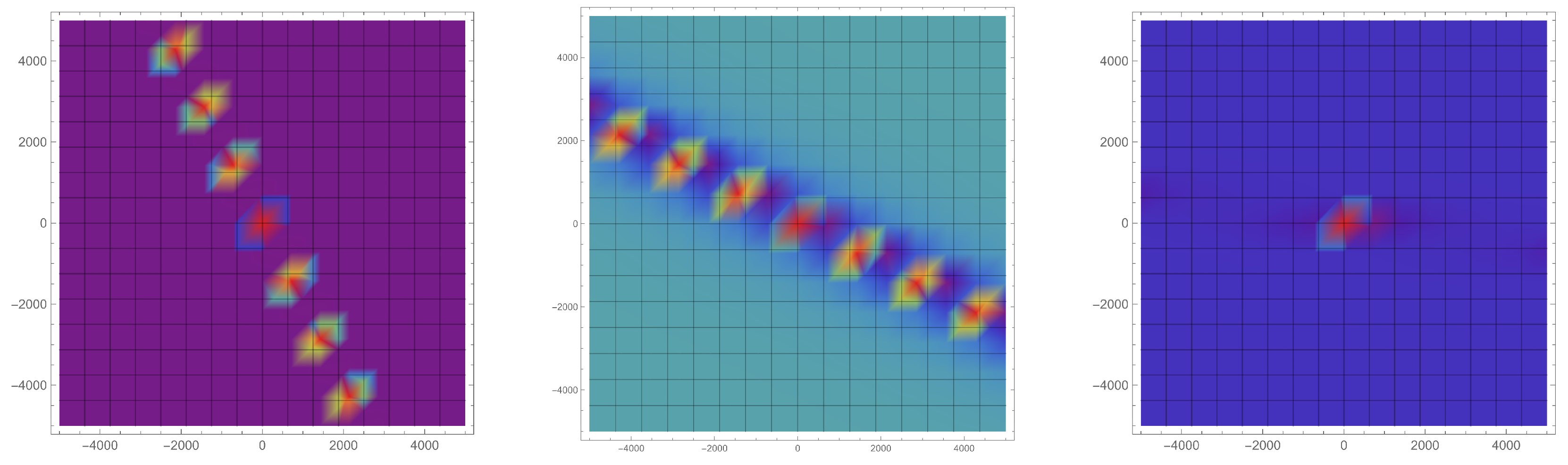
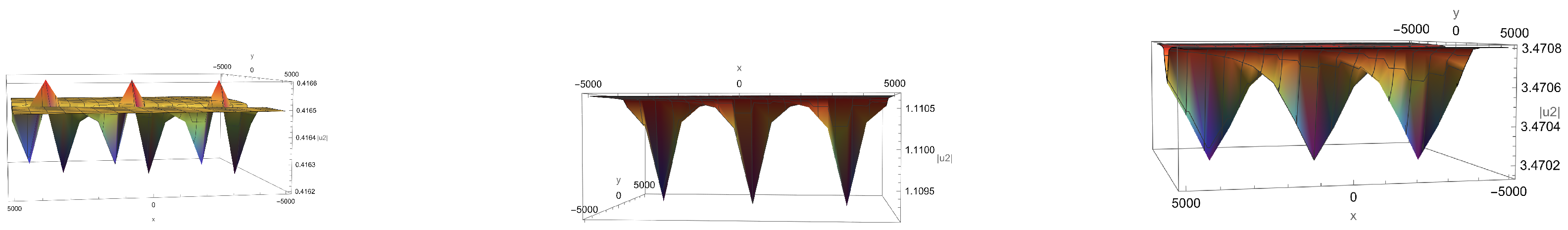
The provided images display both 3D surface plots and density plots created using Mathematica. These visualizations utilize a “Rainbow” color function to map the height (i.e., the absolute value of the function) onto various colors spanning the visible light spectrum. Additionally, a mesh is incorporated for enhanced visualization, allowing for clearer delineation of the function’s topology. The "Rainbow" color function systematically maps different heights of the plot to a gradient of colors, ranging from purple for the lowest values to red for the highest.

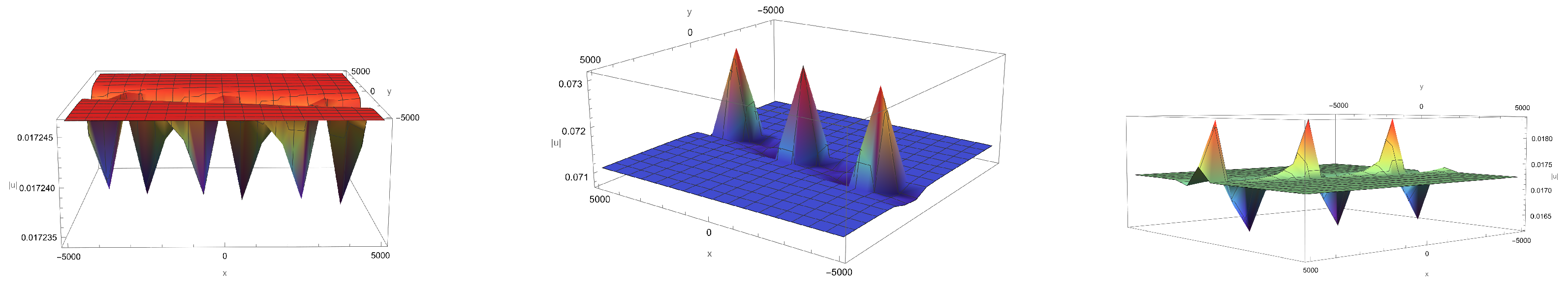
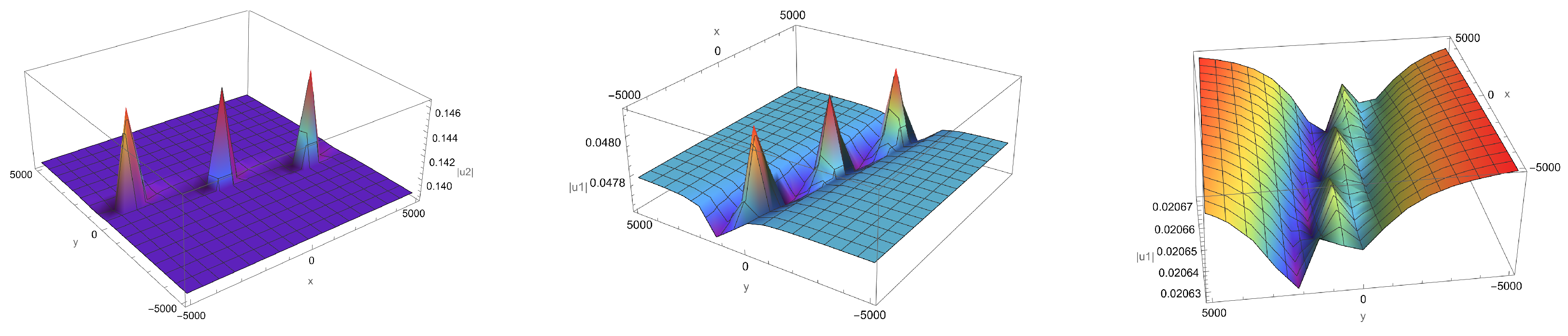
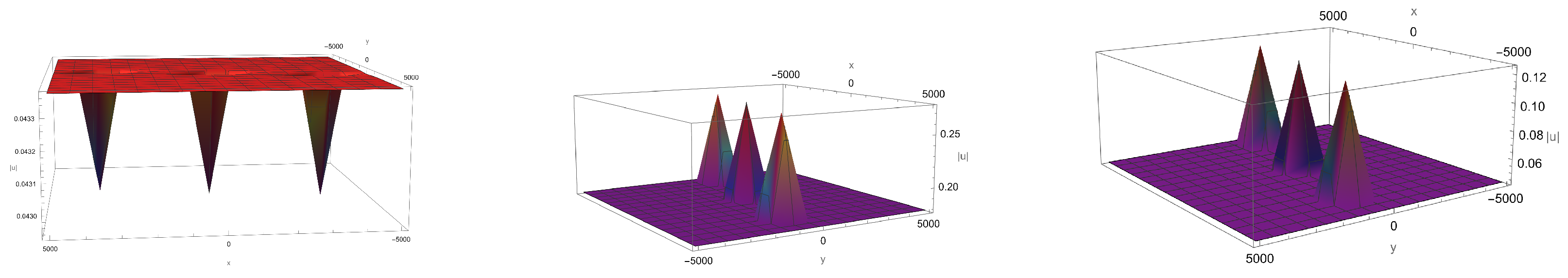
In Figure 3 and Figure 4, we ascend to the second-order bright–dark rogue wave solutions. The increased order introduces more complex wave structures. The peaks and troughs are more pronounced, and the interaction between the bright and dark elements becomes more dynamic, reflecting a more complicated energy distribution within the wave system.

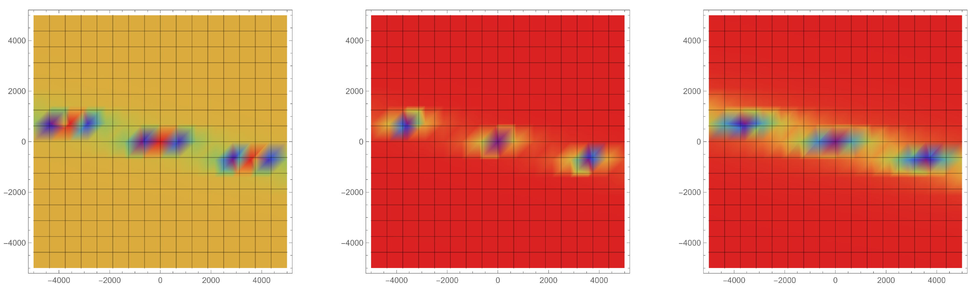
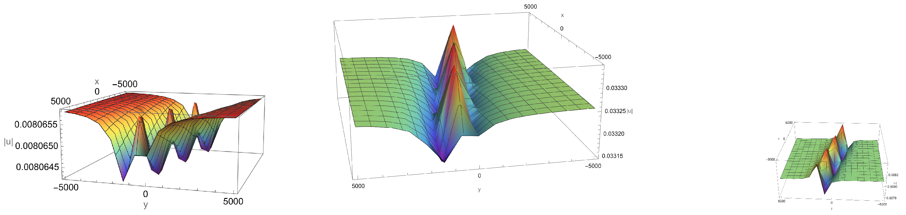
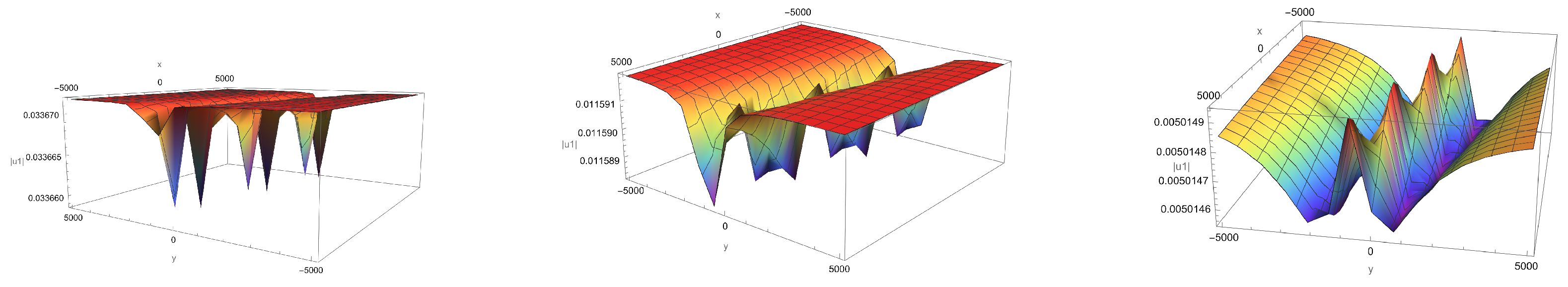
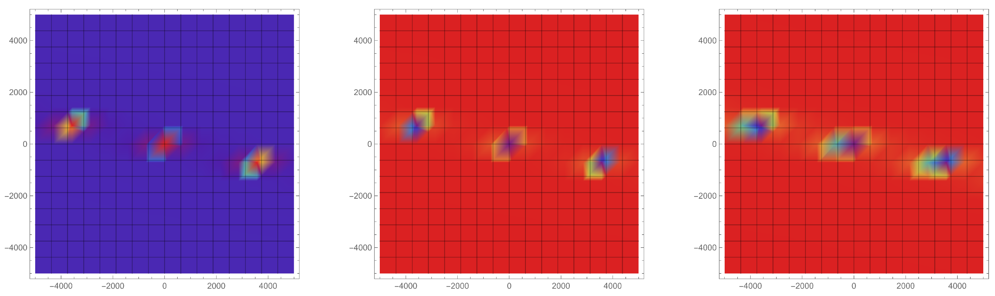
Figure 5 and Figure 6 present the third-order bright–dark rogue wave solutions. The complexity further escalates, displaying an intricate pattern of wave propagation. These higher-order solutions indicate the presence of multiple rogue wave peaks, embodying a system where high-energy concentration areas and points of minimal energy alternate in a complex but systematic manner.

From Figure 1, Figure 2, Figure 3, Figure 4, Figure 5 and Figure 6, a multifaceted evolution of bright–dark rogue waves is depicted, showcasing the intricate interplay between system parameters and the physical properties of the waves. As time progresses, we observe not only an expansion in the spatial range over which the rogue waves propagate, indicating diffusion, but also a noticeable diminution in their peak amplitude. This diminishing amplitude is indicative of energy redistribution within the wave system.

Figure 7 and Figure 8 vividly capture the profound effect of the parameter $\gamma$ on the formation and characteristics of second-order bright–dark rogue waves. The three-dimensional and density plots both articulate how $\gamma$ governs the emergence, spatial positioning, and amplitude metrics relative to the background energy level of the waves. A diminutive $\gamma$ is seen to correlate with an escalated quantity of rogue wave formations, each manifesting with a pronounced amplitude. This is indicative of $\gamma$’s role in enhancing the nonlinearity of the system; a smaller $\gamma$ intensifies the nonlinearity, resulting in a more robust rogue wave occurrence, characterized by heightened peaks that starkly contrast against the surrounding sea state.

Specifically, the plots demonstrate a scenario where the waves, under a lower $\gamma$ value, appear tightly packed and energetically superior, suggesting a state of increased wave interaction and energy transfer. This visually translates into a strikingly varied landscape of peaks and troughs. Conversely, a larger $\gamma$ value scatters the rogue waves, reducing their amplitude and presenting a calmer wave field, indicative of weaker nonlinearity and diminished wave interaction.

Figure 9 and Figure 10 allow for an assessment of the parameter $c_1$’s subtle and nuanced role in the evolution of bright–dark rogue waves. The increment in $c_1$ is observed to marginally nudge the progression between bright and dark rogue waves and mildly bolster the amplitude of these waveforms. Notably, these adjustments are slight, underpinning the robustness and stability of the rogue wave structure against variations in $c_1$. Despite a range of $c_1$ values, the overall silhouette and spatial configuration of the rogue waves exhibit a striking steadfastness. The constancy in shape underscores the inherent stability of the wave formation process, suggesting that the physical mechanisms dictating the rogue wave formation are relatively insensitive to the scaling factor introduced by $c_1$.

This observation reinforces the understanding that while certain system parameters may offer fine adjustments to wave characteristics, the fundamental properties of rogue waves—such as their spatial distribution and essential structure—are resilient to these parameter changes. The persistence of the wave form, despite the varying $c_1$, underscores the dominance of other physical forces and parameters at play, which more profoundly shape the rogue wave phenomenon.

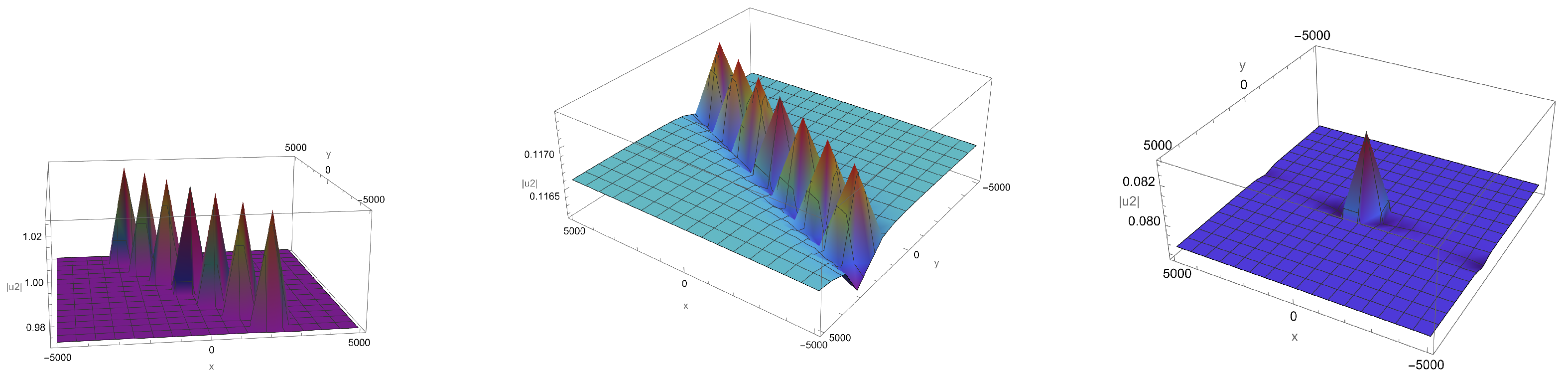
Figure 11 and Figure 12 elucidate the pivotal role of the parameter $c_2$ in dictating the configuration and spatial extent of second-order dark rogue waves. These figures, comprising both three-dimensional plots and density plots, indicate that variations in $c_2$ subtly refine the distribution and breadth of dark rogue wave formations. Specifically, an increment in $c_2$ is associated with a modest increase in the prevalence of dark rogue wave occurrences, leading to a fusion of adjacent waves and thereby broadening the overall expanse of the dark regions within the wave profile.

This gentle increase in $c_2$ facilitates a discernible consolidation among individual dark rogue waves, contributing to a wider collective wave structure without drastically altering the overall wave pattern. Such behavior exemplifies the nuanced influence of $c_2$ on the dark rogue waves’ morphology, reinforcing its role as a fine-tuning parameter within the dynamical system. The essence of this effect is a controlled expansion of the dark regions, effectively changing the wave’s visual and physical presence while preserving the integrity of the individual wave features.

In Figure 13 and Figure 14, the parameter $c_3$ is exhibited as a determinant factor in the morphological transition from bright to dark rogue waves, providing a visualization of how variations in $c_3$ lead to observable changes in the waves’ features. The three-dimensional and density plots together demonstrate that, with an increase in $c_3$, there is a notable shift in the morphology of the rogue wave field, fostering the evolution of wave features from bright, high-energy peaks to dark troughs that are less pronounced in amplitude.

This transition, while visually striking, does not correspond with an alteration in the amplitude of the individual waves; rather, the changes are contained within the visual form and distribution of the rogue waves. The plots illustrate that the secondary waves—additional wave structures that appear alongside the primary rogue wave peaks—adapt their shapes in response to $c_3$ without a concurrent increase or decrease in peak amplitude. This implies a remarkable stability in the wave energy distribution despite the evolving appearance of the waves across the parameter changes.

Figure 15 and Figure 16 showcase the influence of $c_4$ on the morphological characteristics of bright–dark rogue waves, with the parameter exerting a moderate influence on the transition dynamics. The visualization provided by the three-dimensional and density plots indicates that $c_4$ assists in the evolution from bright to dark features within the wave pattern. While this assistance is evident, it operates within the bounds of the existing wave structure, contributing to but not decisively determining the overall wave morphology.

Despite $c_4$’s involvement in the evolution process, the amplitude of the rogue waves exhibits resilience to these parameter changes, maintaining a relative constancy that suggests an underlying robustness in the system. The parameter $c_4$ thus appears to refine the features of the waves subtly, affecting their appearance and the smoothness of their transitions without eliciting a profound change in their peak energies.

Next, we will discuss the influence of variable coefficients on the dynamics of bright–dark rogue waves.

Figure 17, Figure 18, Figure 19 and Figure 20 collectively illustrate the substantial influence of variable coefficients on the formation and evolution of first-, second-, and third-order bright–dark rogue waves. For simplifying the numerical simulation of the solutions, despite the constant value of $a_1\left(t\right)$, the variation in $a_2\left(t\right)$ introduces distinct dynamic behaviors in the waveforms. Employing a single variable coefficient $a_2$ suffices to illustrate the impact of coefficients on wave dynamics.

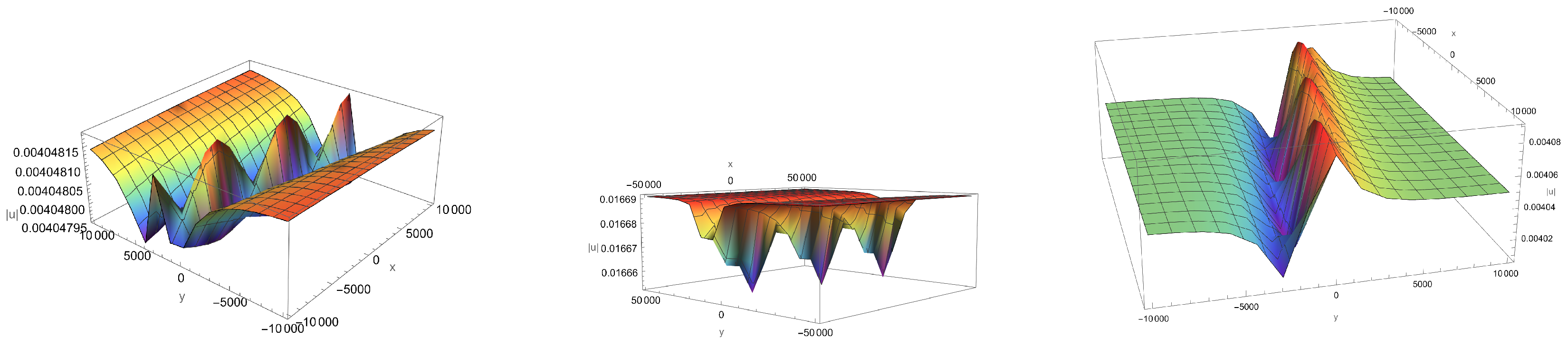
In Figure 17, the linear variation in $a_2\left(t\right)$ introduces a scaling effect on the waves and results in a proportionate spatial modulation of the wave features, with each order exhibiting an adjusted pattern that reflects the linear growth of the coefficient. Figure 18 demonstrates the rogue waves under a quadratic coefficient. At the same time instance, the higher-order influence of $a_2\left(t\right)$ manifests in a more accentuated transformation of the wave patterns. The first-order waves show a subtle increase in peak sharpness compared to the linear case, whereas the higher-order waves, especially the third-order, display a more pronounced spatial complexity. The crests and troughs become more distinct with increased peak steepness and trough depth, suggesting a nonlinear amplification effect on the spatial features of the waves due to the quadratic nature of $a_2\left(t\right)$.

Figure 19 introduces a sinusoidal variation in $a_2\left(t\right)$ with $sin\left(t\right)$, leading to periodic modulations in the waveforms. This sinusoidal factor causes the rogue waves to exhibit a rhythmic pattern in their height and spatial distribution, reflecting the oscillatory modulation imposed by $a_2\left(t\right)$. Finally, Figure 20, with an exponential function $e^t$ defining $a_2\left(t\right)$, shows an intense and accelerating alteration in the wave structures. The waves now display a rapid increase in both the height and complexity, highlighting an exponential sensitivity to the temporal coefficient.

This sequence of figures reveals that the temporal behavior of $a_2\left(t\right)$ significantly influences the rogue waves’ spatial and temporal characteristics. The degree of change ranges from linear stretching and broadening to oscillatory modulation and exponential amplification, illustrating the responsive nature of rogue wave structures to the time-dependent changes in system parameters.

5. Conclusions

This paper has focused on the (2+1)-dimensional variable-coefficient Zakharov equation and has successfully constructed high-order bright–dark rogue wave solutions through the self-similar transformation and Darboux transformation. The research has demonstrated that these solutions can reveal the complex dynamics of energy concentration and energy dissipation in nonlinear wave propagation in oceanic rogue waves. Through the dynamic analysis of the propagation characteristics of rogue waves, this study has elucidated the significant influence of system parameters and variable coefficient selection on the waveform shape, amplitude, and evolution process. It has been particularly found that the selection of variable coefficients can significantly alter the shape of the waveform, while adjustments to the constant parameters have affected the number, position, and relationship with the background level of the rogue waves. Furthermore, the physical implications of these findings extend to practical scenarios where understanding and predicting the behavior of rogue waves can be crucial. For instance, the ability to manipulate wave characteristics through parameter adjustments provides valuable insights for designing maritime structures resilient to such extreme conditions. This ability highlights the direct applicability of mathematical transformations in engineering practices aimed at reducing risks associated with high-energy wave events.

The innovative points of this paper are as follows: This paper, with the help of the method given in the literature [10], has, for the first time, successfully constructed high-order bright–dark rogue wave solutions in the (2+1)-dimensional variable-coefficient Zakharov equation through the self-similar transformation and Darboux transformation, providing a new analytical tool for understanding nonlinear wave phenomena. Through numerical simulation and theoretical analysis, this paper has deeply explored the dynamic behavior of rogue wave propagation characteristics, especially the impact of variable coefficients on rogue wave morphology, which has rarely been involved in previous research. This paper has shown the relationship between rogue wave characteristics (such as number, amplitude, morphology, etc.) and system parameters (such as constant parameters $c_i$, $\lambda$ and variable coefficients $a_j\left(t\right)$), providing theoretical guidance for the control and modulation of nonlinear wave motion. Through detailed parameter research and image display, this paper has comprehensively shown the evolution process of rogue waves under the influence of multiple factors, providing a perspective for a deep understanding of the dynamic behavior of nonlinear wave motion.

Compared with the literature [10], this paper has applied the self-similar transformation to the (2+1)-dimensional variable-coefficient Zakharov equation for the first time, and has studied the impact of variable coefficients on bright–dark rogue wave solutions. The literature [10] only studied the low-order linear rogue wave cluster of the constant coefficient Zakharov equation, and this paper has studied the high-order bright–dark rogue wave solution of the (2+1)-dimensional variable-coefficient Zakharov equation. The literature [10] indirectly studied the propagation characteristics of the Zakharov equation with the help of the rogue wave solution of the degenerated NLS equation, and this paper has directly studied the impact of various parameters on the high-order bright–dark rogue wave solution of the (2+1)-dimensional variable-coefficient Zakharov equation.

In summary, this research has not only enriched the types of solutions of the (2+1)-dimensional variable-coefficient Zakharov equation in theory but has also provided new ideas and tools for the analysis and control of nonlinear wave motion in methodology, which holds important academic value and application potential.