
Instance Segmentation of Sparse Point Clouds with Spatio-Temporal Coding for Autonomous Robot

Abstract
1. Introduction
2. Related Work
2.1. Point Clouds Instance Segmentation
2.2. Autonomous Robot Dynamic Environment Target Filtering
3. Methods
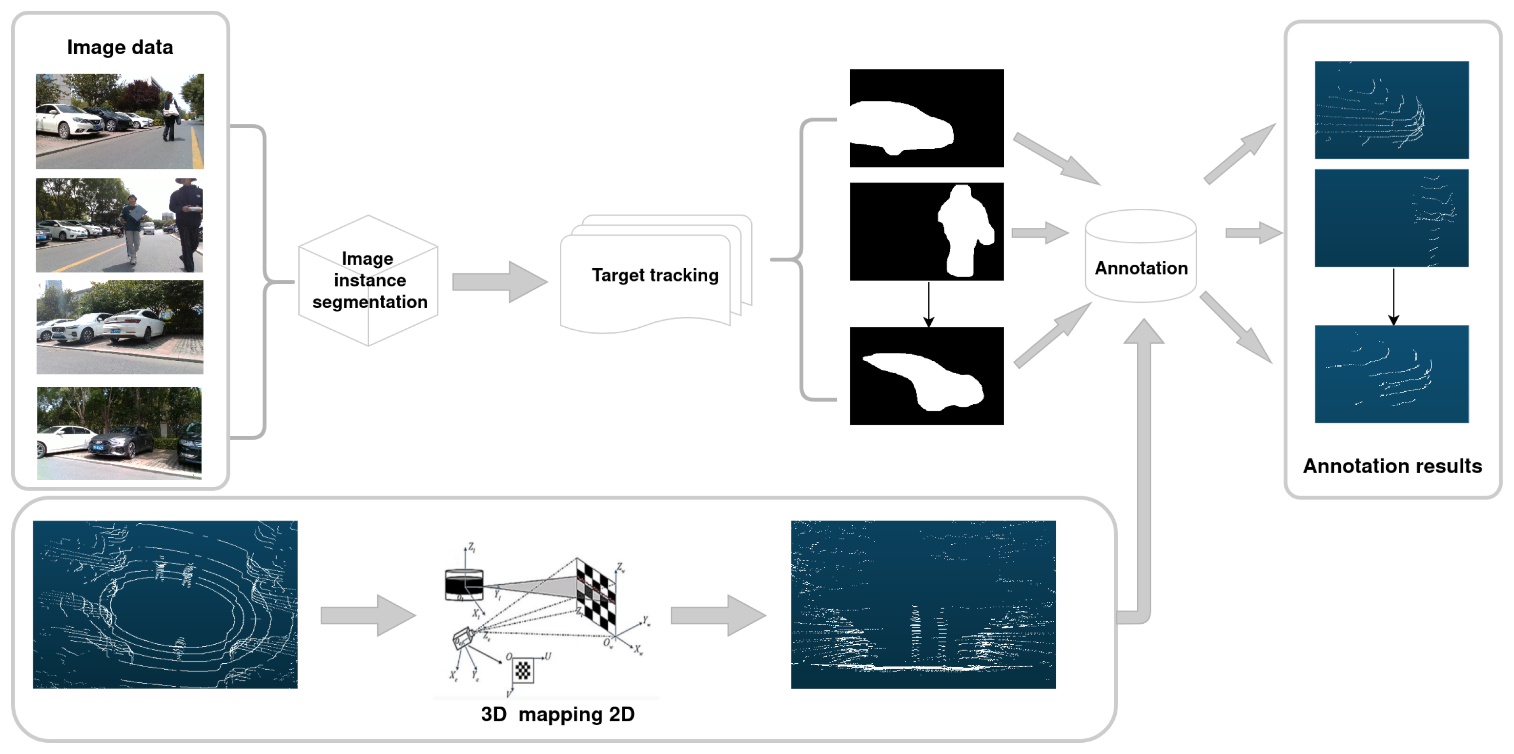
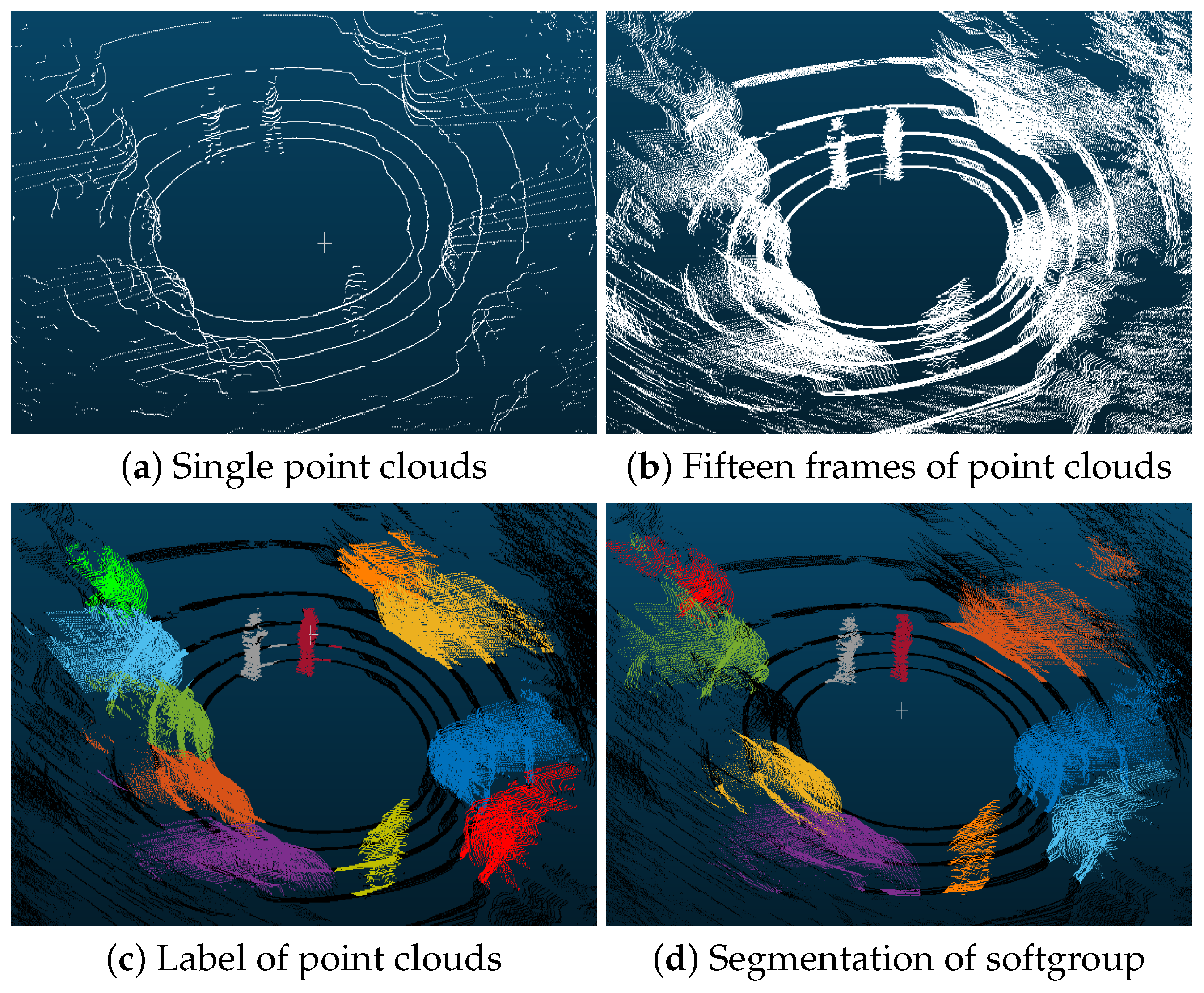
3.1. Automatic Data Annotation
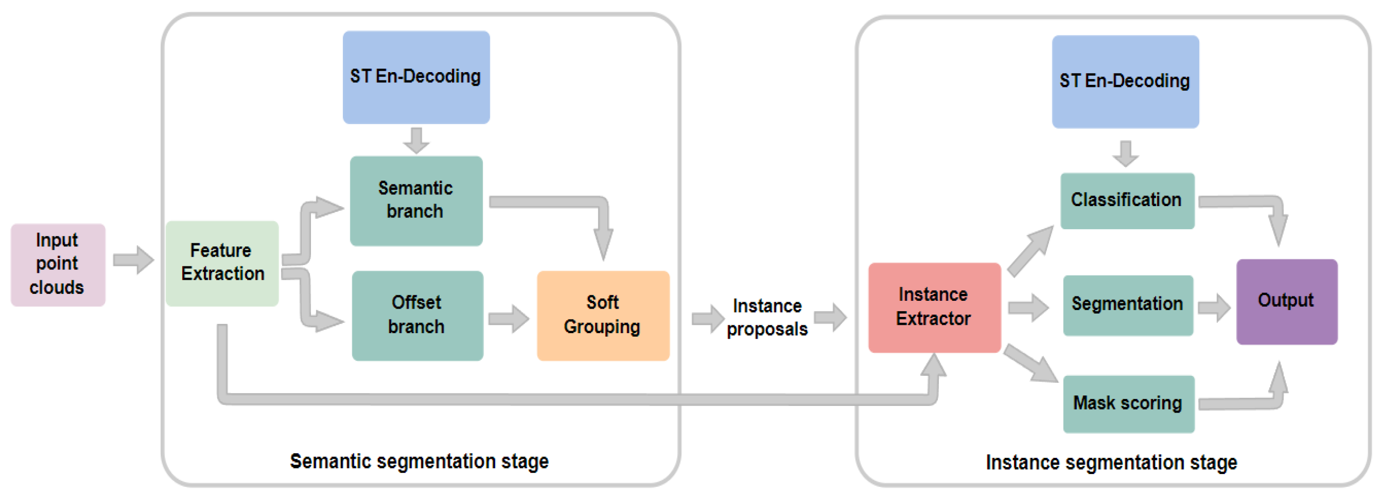
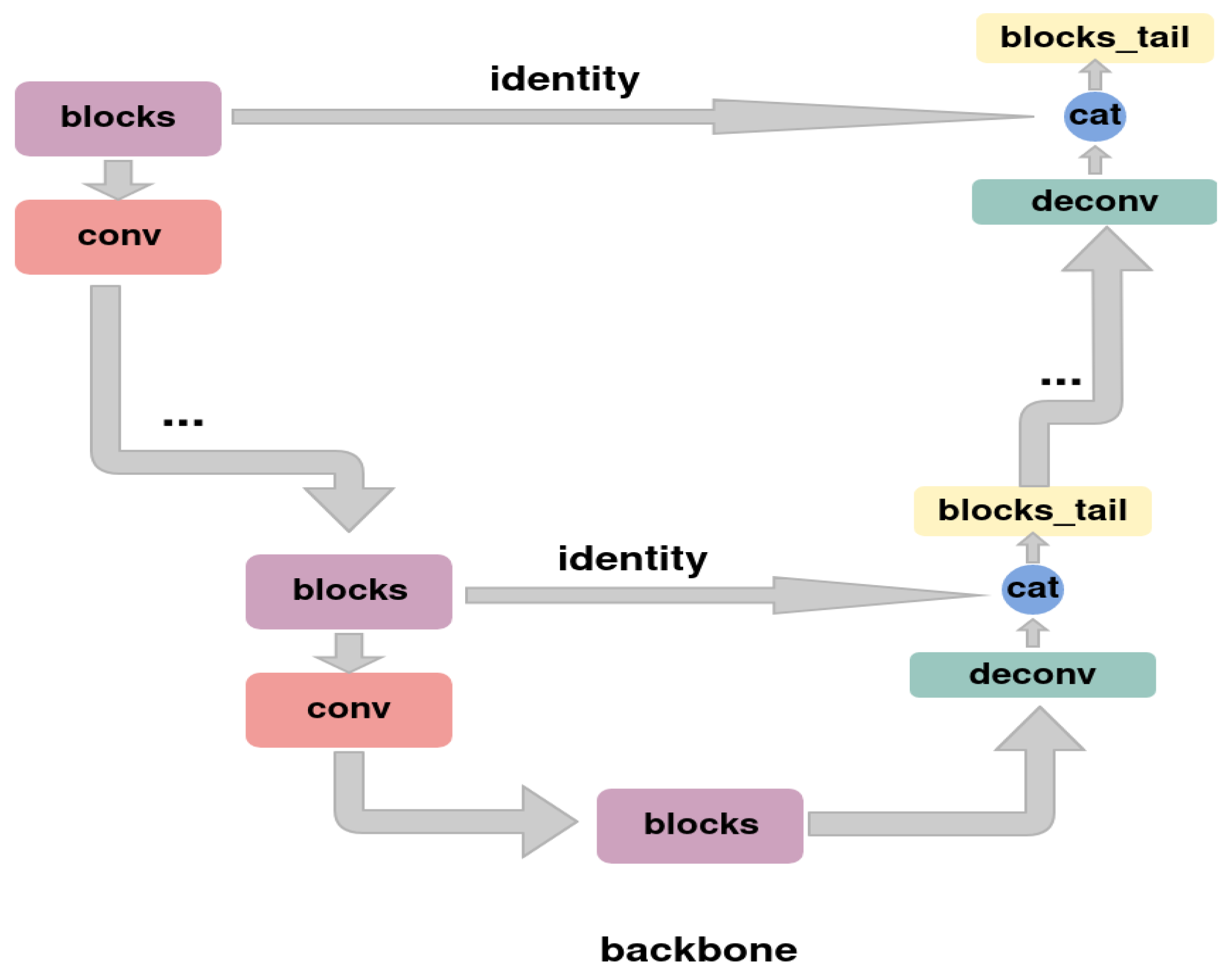
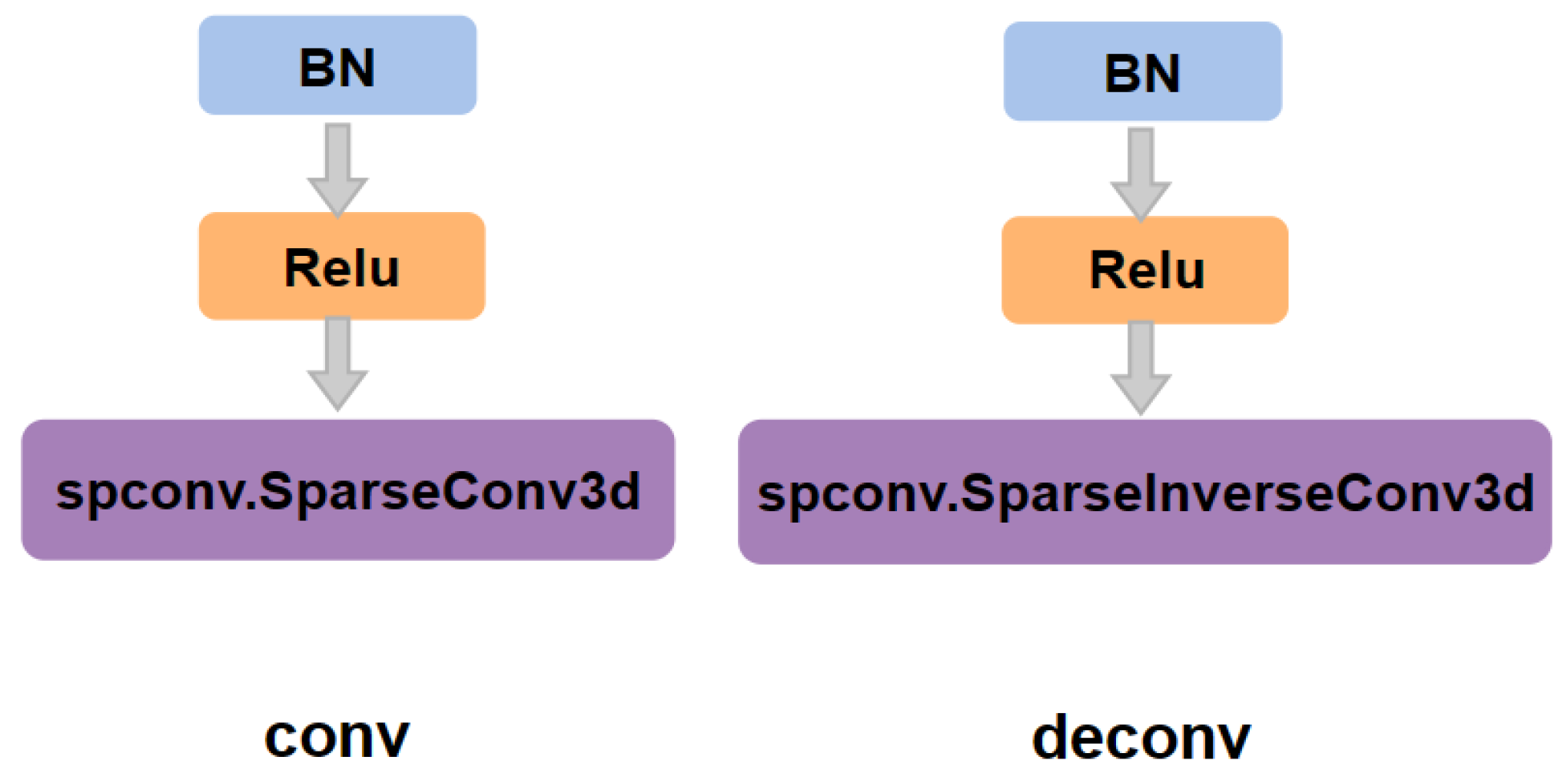
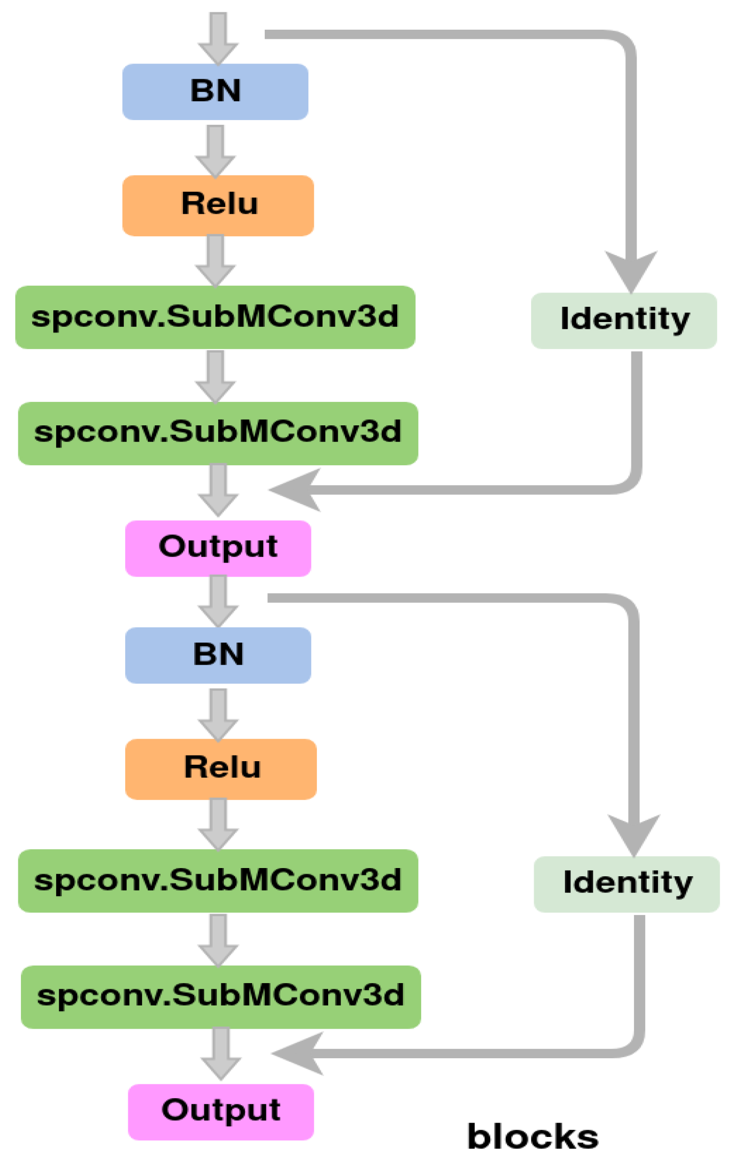
3.2. Proposed Instance Segmentation
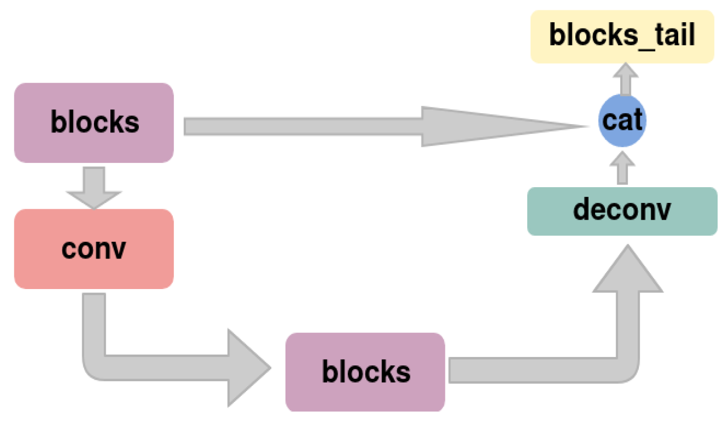
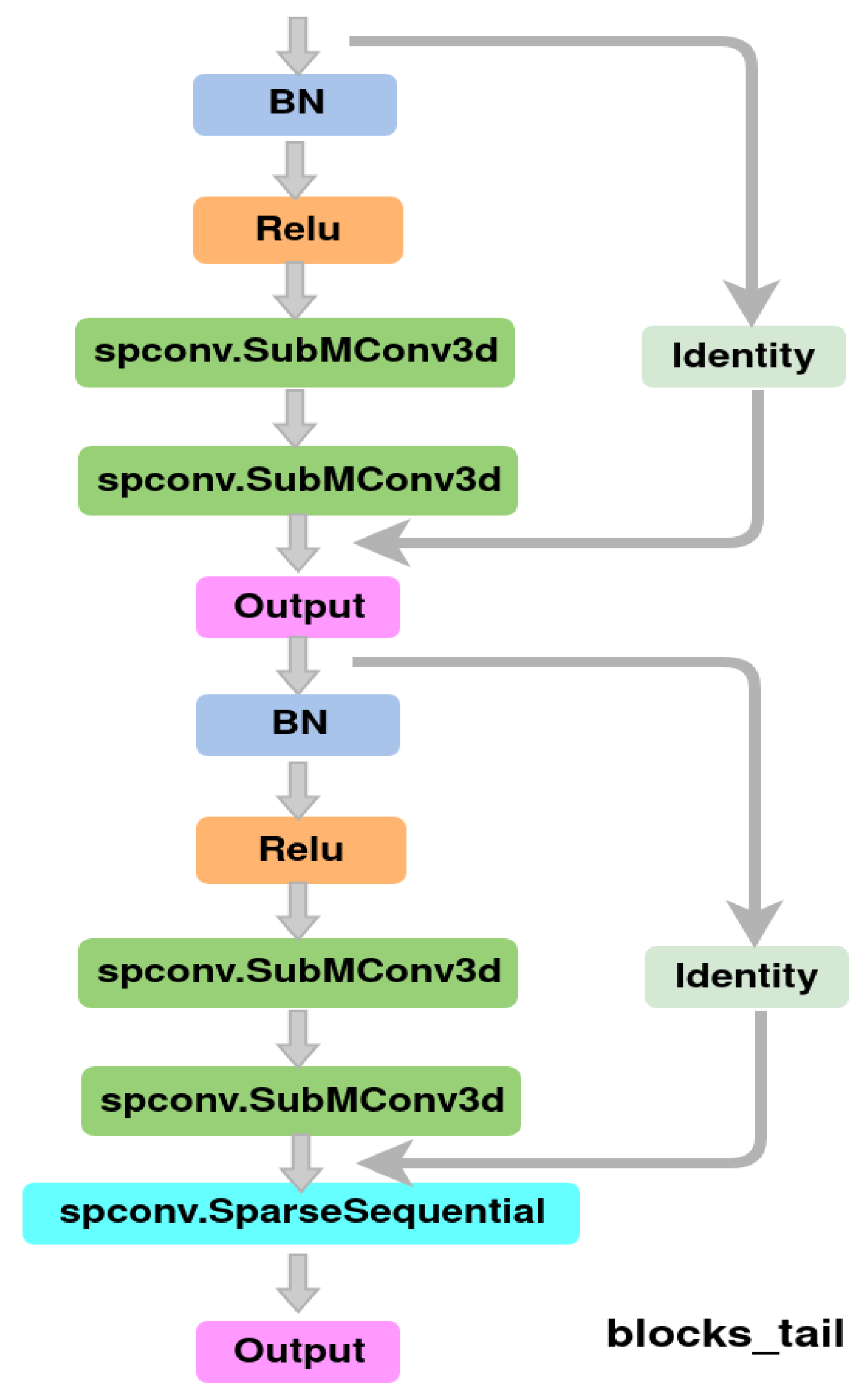
3.3. Spatio-Temporal Encoding and Decoding
4. Experiments
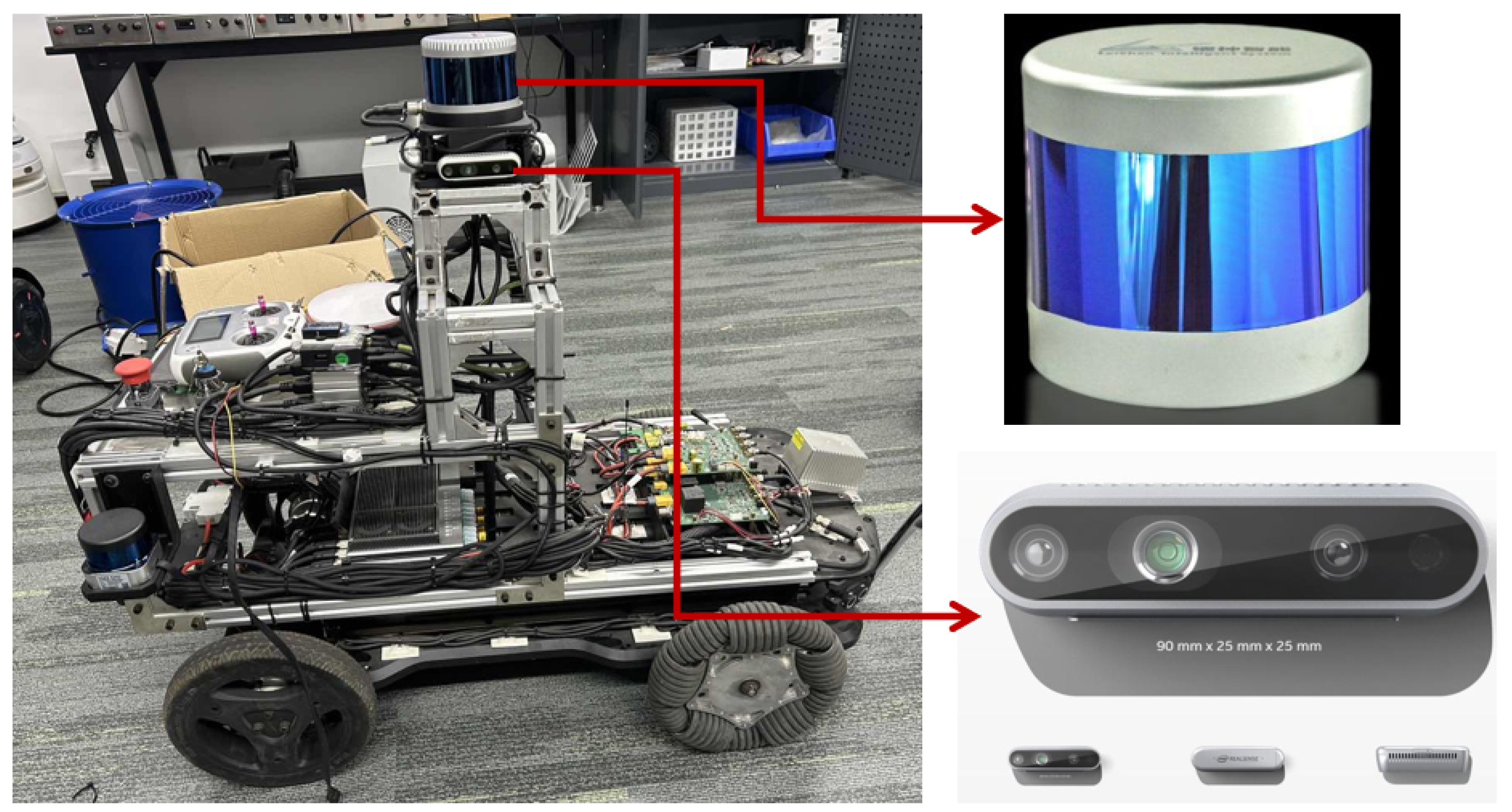
4.1. Autonomous Robot Hardware Settings
4.2. Dataset
4.3. Experiments and Discussions
5. Conclusions
Author Contributions
Funding
Data Availability Statement
Conflicts of Interest
References
- Tixiao, S.; Brendan, E.; Drew, M.; Wei, W.; Carlo, R.; Daniela, R. LIO-SAM: Tightly-coupled Lidar Inertial Odometry via Smoothing and Mapping. In Proceedings of the IEEE/RSJ International Conference on Intelligent Robots and Systems (IROS), Las Vegas, LA, USA, 25–29 October 2020; IEEE: Piscataway, NJ, USA, 2020; pp. 5135–5142. [Google Scholar]
- Cadena, C.; Carlone, L.; Carrillo, H.; Latif, Y.; Scaramuzza, D.; Neira, J.; Reid, I.D.; Leonard, J.J. Simultaneous localization and mapping: Present, future, and the robust-perception age. arXiv 2016, arXiv:1606.05830. [Google Scholar] [CrossRef]
- Kim, G.; Kim, A. Remove, then Revert: Static point clouds Map Construction using Multiresolution Range Images. In Proceedings of the IEEE/RSJ International Conference on Intelligent Robots and Systems (IROS), Las Vegas, LA, USA, 25–29 October 2020; IEEE: Piscataway, NJ, USA, 2020; pp. 10758–10765. [Google Scholar] [CrossRef]
- Guo, Y.; Wang, H.; Hu, Q.; Liu, H.; Liu, L.; Bennamoun, M. Deep learning for 3D point clouds: A survey. In Proceedings of the IEEE Transactions on Pattern Analysis and Machine Intelligence, Dubai, United Arab Emirates, 29 June 2020; Volume 43, pp. 4338–4364. [Google Scholar]
- Lahoud, J.; Ghanem, B.; Pollefeys, M.; Oswald, M.R. 3D instance segmentation via multi-task metric learning. In Proceedings of the IEEE/CVF International Conference on Computer Vision, Seoul, Republic of Korea, 27 October–2 November 2019; pp. 9256–9266. [Google Scholar]
- Qian, C.; Xiang, Z.; Wu, Z.; Sun, H. RF-LIO: Removal-First Tightly-coupled Lidar Inertial Odometry in High Dynamic Environments. In Proceedings of the 2021 IEEE/RSJ International Conference on Intelligent Robots and Systems (IROS), Prague, Czech Republic, 27 September–1 October 2021; pp. 4421–4428. [Google Scholar] [CrossRef]
- Pfreundschuh, P.; Hendrikx, H.F.; Reijgwart, V.; Dubé, R.; Siegwart, R.; Cramariuc, A. Dynamic object aware lidar slam based on automatic generation of training data. In Proceedings of the 2021 IEEE International Conference on Robotics and Automation (ICRA), Xi’an, China, 30 May–5 June 2021; pp. 11641–11647. [Google Scholar]
- Yoon, D.; Tang, T.; Barfoot, T. Mapless online detection of dynamic objects in 3D lidar. In Proceedings of the 16th Conference on Computer and Robot Vision, Kingston, QC, Canada, 29–31 May 2019. [Google Scholar]
- Schauer, J.; Nüchter, A. The Peopleremover—Removing Dynamic Objects From 3-D point clouds by Traversing a Voxel Occupancy Grid. IEEE Robot. Autom. Lett. 2018, 3, 1679–1686. [Google Scholar] [CrossRef]
- Lim, H.; Hwang, S.; Myung, H. ERASOR: Egocentric Ratio of Pseudo Occupancy-Based Dynamic Object Removal for Static 3D point clouds Map Building. IEEE Robot. Autom. Lett. 2021, 6, 2272–2279. [Google Scholar] [CrossRef]
- Kim, G.; Kim, A. LT-mapper: A Modular Framework for LiDAR-based Lifelong Mapping. In Proceedings of the 2022 International Conference on Robotics and Automation (ICRA), Philadelphia, PA, USA, 23–27 May 2022; pp. 7995–8002. [Google Scholar]
- Pomerleau, F.; Krüsi, P.; Colas, F.; Furgale, P.; Siegwart, R. Long-term 3D map maintenance in dynamic environments. In Proceedings of the 2014 IEEE International Conference on Robotics and Automation (ICRA), Hong Kong, China, 31 May–7 June 2014; pp. 3712–3719. [Google Scholar] [CrossRef]
- Milioto, A.; Vizzo, I.; Behley, J.; Stachniss, C. Rangenet++: Fast and accurate lidar semantic segmentation. In Proceedings of the 2019 IEEE/RSJ International Conference on Intelligent Robots and Systems (IROS), Kyoto, Japan, 23–27 October 2022; IEEE: Piscataway, NJ, USA, 2019; pp. 4213–4220. [Google Scholar]
- Yi, L.; Zhao, W.; Wang, H.; Sung, M.; Guibas, L. GSPN: Generative Shape Proposal Network for 3D Instance Segmentation in point clouds. In Proceedings of the 2019 IEEE/CVF Conference on Computer Vision and Pattern Recognition (CVPR), Long Beach, CA, USA, 15–20 June 2019; pp. 3942–3951. [Google Scholar] [CrossRef]
- Hou, J.; Dai, A.; Nießner, M. 3D-SIS: 3D Semantic Instance Segmentation of RGB-D Scans. In Proceedings of the 2019 IEEE/CVF Conference on Computer Vision and Pattern Recognition (CVPR), Long Beach, CA, USA, 15–20 June 2019; pp. 4421–4430. [Google Scholar] [CrossRef]
- Yang, B.; Wang, J.; Clark, R.; Hu, Q.; Wang, S.; Markham, A.; Trigoni, N. Learning Object Bounding Boxes for 3D Instance Segmentation on point clouds. In Proceedings of the 2019 Conference on Computer Vision and Pattern Recognition, Long Beach, CA, USA, 15–20 June 2019. [Google Scholar]
- Liu, S.H.; Yu, S.Y.; Wu, S.C.; Chen, H.T.; Liu, T.L. Learning gaussian instance segmentation in point clouds. arXiv 2020, arXiv:2007.09860. [Google Scholar]
- Valada, A.; Vertens, J.; Dhall, A.; Burgard, W. Adapnet: Adaptive semantic segmentation in adverse environmental conditions. In Proceedings of the 2017 IEEE International Conference on Robotics and Automation, Singapore, 29 May–3 June 2017; pp. 4644–4651. [Google Scholar]
- Chabot, F.; Chaouch, M.; Rabarisoa, J.; Teuliere, C.; Chateau, T. Deep manta: A coarse-to-fine many-task network for joint 2D and 3D vehicle analysis from monocular image. In Proceedings of the IEEE conference on computer vision and pattern recognition (pp. 2040–2049). arXiv 2017, arXiv:1703.07570. [Google Scholar]
- Dewan, A.; Oliveira, G.L.; Burgard, W. Deep semantic classification for 3D lidar data. In 2017 IEEE/RSJ International Conference on Intelligent Robots and Systems (IROS) (pp. 3544–3549). arXiv 2017, arXiv:1706.08355. [Google Scholar]
- Engelcke, M.; Rao, D.; Wang, D.Z.; Tong, C.H.; Posner, I. Vote3Deep: Fast object detection in 3D point clouds using efficient convolutional neural networks. In Proceedings of the 2017 IEEE International Conference on Robotics and Automation (ICRA), Singapore, 29 May–3 June 2017; pp. 1355–1361. [Google Scholar]
- Li, B.; Zhang, T.; Xia, T. Vehicle detection from 3D lidar using fully convolutional network. arXiv 2016, arXiv:1608.07916. [Google Scholar]
- Reddy, N.D.; Singhal, P.; Krishna, K.M. Semantic motion segmentation using dense crf formulation. In Proceedings of the 2014 Indian Conference on Computer Vision Graphics and Image Processing, ACM, Bangalore, India, 14–18 December 2014; p. 56. [Google Scholar]
- Vertens, J.; Valada, A.; Burgard, W. Smsnet: Semantic motion segmentation using deep convolutional neural networks. In Proceedings of the IEEE/RSJ International Conference on Intelligent Robots and Systems, IROS, Vancouver, BC, Canada, 24–28 September 2017. [Google Scholar]
- Chen, X.; Ma, H.; Wan, J.; Li, B.; Xia, T. Multi-view 3D object detection network for autonomous driving. In Proceedings of the IEEE conference on Computer Vision and Pattern Recognition (pp. 1907–1915). arXiv 2016, arXiv:1611.07759. [Google Scholar]
- Xu, J.; Kim, K.; Zhang, Z.; Chen, H.W.; Owechko, Y. 2D/3D sensor exploitation and fusion for enhanced object detection. In Proceedings of the Computer Vision and Pattern Recognition Workshops (CVPRW, pp. 764–770), Columbus, OH, USA, 23–28 June 2014; pp. 778–784. [Google Scholar]
- Wang, D.Z.; Posner, I. Voting for voting in online point clouds object detection. Robot. Sci. Syst. 2015, 1, 10–15. [Google Scholar]
- Hahnel, D.; Triebel, R.; Burgard, W.; Thrun, S. Map building with mobile robots in dynamic environments. In Proceedings of the 2003 IEEE International Conference on Robotics and Automation (Cat. No. 03CH37422), Taipei, Taiwan, 12–17 May 2003; Volume 2, pp. 1557–1563. [Google Scholar]
- Meyer-Delius, D.; Beinhofer, M.; Burgard, W. Occupancy grid models for robot mapping in changing environments. In Proceedings of the AAAI Conference on Artificial Intelligence, Atlanta, GA, USA, 11–15 July 2012; Volume 26, pp. 2024–2030. [Google Scholar]
- Ronneberger, O.; Fischer, P.; Brox, T. Unet: Convolutional networks for biomedical image segmentation. In Medical Image Computing and Computer-Assisted Intervention, Proceedings of the MICCAI 2015: 18th International Conference, Munich, Germany, 5–9 October 2015, Proceedings, Part III 18; Springer International Publishing: Berlin/Heidelberg, Germany, 2015; pp. 234–241. [Google Scholar]
- Graham, B.; Engelcke, M.; Maaten, L.V. 3D semantic segmentation with submanifold sparse convolutional networks. In Proceedings of the IEEE Conference on Computer Vision and Pattern Recognition, Salt Lake City, UT, USA, 18–23 June 2018; pp. 9224–9232. [Google Scholar]
- Chen, S.; Fang, J.; Zhang, Q.; Liu, W.; Wang, X. Hierarchical aggregation for 3D instance segmentation. In Proceedings of the IEEE/CVF International Conference on Computer Vision, Montreal, BC, Canada, 11–17 October 2021; pp. 15467–15476. [Google Scholar]
- Jiang, L.; Zhao, H.; Shi, S.; Liu, S.; Fu, C.W.; Jia, J. Pointgroup: Dual-set point grouping for 3D instance segmentation. In Proceedings of the IEEE/CVF Conference on Computer Vision and Pattern Recognition, Seattle, WA, USA, 13–19 June 2020; pp. 4867–4876. [Google Scholar]
- Liang, Z.; Li, Z.; Xu, S.; Tan, M.; Jia, K. Instance segmentation in 3D scenes using semantic superpoint tree networks. In Proceedings of the IEEE/CVF International Conference on Computer Vision, Montreal, BC, Canada, 11–17 October 2021; pp. 2783–2792. [Google Scholar]
- He, K.; Gkioxari, G.; Dollár, P.; Girshick, R. Mask r-cnn. In Proceedings of the IEEE International Conference on Computer Vision, Venice, Italy, 22–29 October 2017; pp. 2961–2969. [Google Scholar]
- Huang, Z.; Huang, L.; Gong, Y.; Huang, C.; Wang, X. Mask scoring r-cnn. In Proceedings of the IEEE/CVF Conference on Computer Vision and Pattern Recognition, Long Beach, CA, USA, 15–20 June 2019; pp. 6409–6418. [Google Scholar]


| Framerate | 5 | 9 | 13 | 15 |
|---|---|---|---|---|
| type | car | car | car | car |
| AP_25 | 0.608 | 0.701 | 0.733 | 0.783 |
| AP_50 | 0.477 | 0.487 | 0.656 | 0.704 |
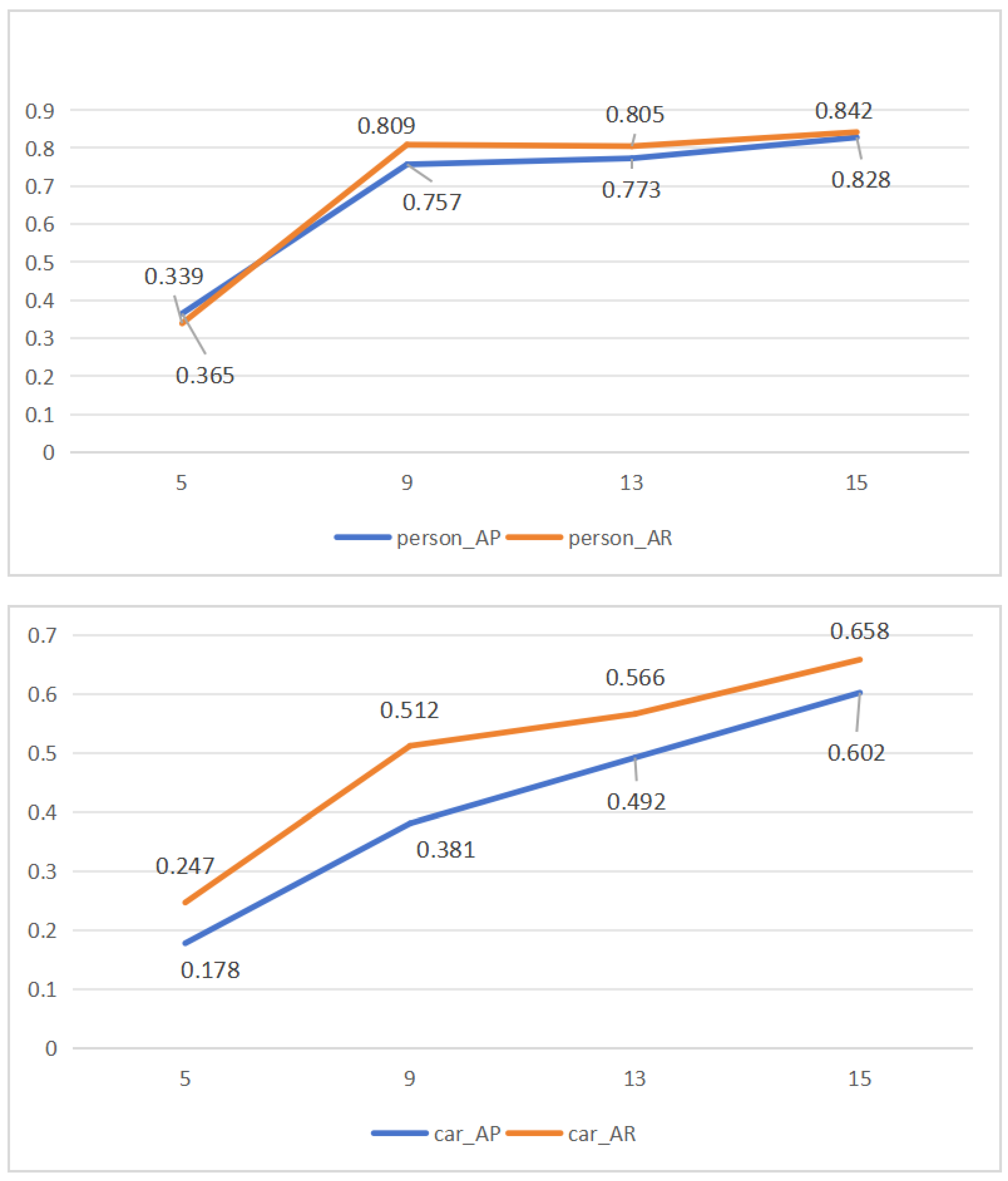
| AP | 0.178 | 0.381 | 0.492 | 0.602 |
| RC_25 | 0.644 | 0.783 | 0.849 | 0.879 |
| RC_50 | 0.525 | 0.655 | 0.797 | 0.807 |
| AR | 0.247 | 0.512 | 0.566 | 0.658 |
| Framerate | 5 | 9 | 13 | 15 |
|---|---|---|---|---|
| type | person | person | person | person |
| AP_25 | 0.577 | 0.814 | 0.821 | 0.905 |
| AP_50 | 0.528 | 0.759 | 0.816 | 0.871 |
| AP | 0.365 | 0.757 | 0.773 | 0.828 |
| RC_25 | 0.635 | 0.898 | 0.898 | 0.910 |
| RC_50 | 0.584 | 0.810 | 0.876 | 0.881 |
| AR | 0.339 | 0.809 | 0.805 | 0.842 |
| Framerate | 5 | 9 | 13 | 15 |
|---|---|---|---|---|
| type | car + person | car + person | car + person | car + person |
| AP_25 | 0.592 | 0.757 | 0.777 | 0.844 |
| AP_50 | 0.502 | 0.623 | 0.736 | 0.787 |
| AP | 0.272 | 0.569 | 0.633 | 0.715 |
| RC_25 | 0.639 | 0.840 | 0.873 | 0.894 |
| RC_50 | 0.554 | 0.732 | 0.837 | 0.844 |
| AR | 0.339 | 0.660 | 0.685 | 0.750 |
| Method | Softgroup | Ours |
|---|---|---|
| type | car | car |
| AP_25 | 0.783 | 0.810 |
| AP_50 | 0.704 | 0.767 |
| AP | 0.602 | 0.765 |
| RC_25 | 0.879 | 0.832 |
| RC_50 | 0.807 | 0.802 |
| AR | 0.658 | 0.796 |
| Method | Softgroup | Ours |
|---|---|---|
| type | person | person |
| AP_25 | 0.905 | 0.924 |
| AP_50 | 0.871 | 0.897 |
| AP | 0.828 | 0.887 |
| RC_25 | 0.910 | 0.933 |
| RC_50 | 0.881 | 0.913 |
| AR | 0.842 | 0.907 |
| Method | Softgroup | Ours |
|---|---|---|
| type | car + person | car + person |
| AP_25 | 0.844 | 0.867 |
| AP_50 | 0.787 | 0.832 |
| AP | 0.715 | 0.826 |
| RC_25 | 0.894 | 0.883 |
| RC_50 | 0.844 | 0.857 |
| AR | 0.750 | 0.851 |
Disclaimer/Publisher’s Note: The statements, opinions and data contained in all publications are solely those of the individual author(s) and contributor(s) and not of MDPI and/or the editor(s). MDPI and/or the editor(s) disclaim responsibility for any injury to people or property resulting from any ideas, methods, instructions or products referred to in the content. |
© 2024 by the authors. Licensee MDPI, Basel, Switzerland. This article is an open access article distributed under the terms and conditions of the Creative Commons Attribution (CC BY) license (https://creativecommons.org/licenses/by/4.0/).
Share and Cite
Liu, N.; Yuan, Y.; Zhang, S.; Wu, G.; Leng, J.; Wan, L. Instance Segmentation of Sparse Point Clouds with Spatio-Temporal Coding for Autonomous Robot. Mathematics 2024, 12, 1200. https://doi.org/10.3390/math12081200
Liu N, Yuan Y, Zhang S, Wu G, Leng J, Wan L. Instance Segmentation of Sparse Point Clouds with Spatio-Temporal Coding for Autonomous Robot. Mathematics. 2024; 12(8):1200. https://doi.org/10.3390/math12081200
Chicago/Turabian StyleLiu, Na, Ye Yuan, Sai Zhang, Guodong Wu, Jie Leng, and Lihong Wan. 2024. "Instance Segmentation of Sparse Point Clouds with Spatio-Temporal Coding for Autonomous Robot" Mathematics 12, no. 8: 1200. https://doi.org/10.3390/math12081200
APA StyleLiu, N., Yuan, Y., Zhang, S., Wu, G., Leng, J., & Wan, L. (2024). Instance Segmentation of Sparse Point Clouds with Spatio-Temporal Coding for Autonomous Robot. Mathematics, 12(8), 1200. https://doi.org/10.3390/math12081200