The Gauge Equation in Statistical Manifolds: An Approach through Spectral Sequences

Abstract

The gauge equation is a generalization of the conjugacy relation for the Koszul connection to bundle morphisms that are not isomorphisms. The existence of nontrivial solution to this equation, especially when duality is imposed upon related connections, provides important information about the geometry of the manifolds under consideration. In this article, we use the gauge equation to introduce spectral sequences that are further specialized to Hessian structures.

1. Introduction

The motivation behind this paper is the computation of Koszul–Vinberg cohomology, which is closely related to information geometry through appropriate spectral sequences, resulting in a powerful machinery successfully applied in various problems arising in differential topologies and differential geometries. A Koszul connection [1] can be viewed informally as means for taking the derivative of a section s of a vector bundle $E\to M$, with M being a smooth manifold, along a vector field $X\in TM$. The resulting section is denoted by ${\nabla }_{X}s$, with ∇ as the connection. It defines an $\mathbb{R}$-bilinear product on sections by $s.s^{\prime }={\nabla }_s{s}^{\prime }$ whose commutator is the Lie bracket if ∇ is torsion-free. The associator of the product $(s,s^{\prime },s^{″})=(s.s^{\prime }).s^{″}-s.(s^{\prime }.s^{″})$ can be easily computed as $(s,s^{\prime },s^{″})={\nabla }_{s,s^{\prime }}^2{s}^{″}$, meaning that $(s,s^{\prime },s^{″})-(s,s^{\prime },s^{″})=R(s,s^{\prime })s^{″}$. When the connection ∇ is flat, $(s,s^{\prime },s^{″})-(s,s^{\prime },s^{″})=0$, turning the real vector space of sections into a Koszul–Vinberg algebra, also called a pre-Lie algebra [2]. This fact is used in Section 3 to introduce a cohomology from which spectral sequences of interest arise.

The second key ingredient is an important concept coming from the general theory of Koszul connections is the gauge equation. If ∇ is a Koszul connection on the bundle E and $\theta :E\to E$ is a bundle isomorphism, then ${\theta }^{-1}\nabla \theta$ is a Koszul connection. This defines an action of the gauge group on Koszul connections; when two connections ${\nabla }_1,{\nabla }_2$ are in the same conjugacy class, there exists $\theta$ in the gauge group such that ${\theta }^{-1}{\nabla }_1\theta ={\nabla }_2$, or equivalently, ${\nabla }_1\theta =\theta {\nabla }_2.$ Relaxing the invertibility assumption on $\theta$ gives rise to the so-called gauge equation: two connections ${\nabla }_1,{\nabla }_2$ on a vector bundle $E\stackrel{\pi }{⟶}M$ are said to satisfy a gauge equation if there exists a bundle morphism $\theta :E\to E$ such that ${\nabla }_1\theta =\theta {\nabla }_2.$ Without additional assumptions on ${\nabla }_1,{\nabla }_2$, any global section $\theta$ of $hom(E,E)$ satisfies a gauge equation.

Thus, is thus necessary to place some constraints on the couple $({\nabla }_1,{\nabla }_2)$ in order to obtain useful results. In this paper, we focus on dual connections as provided by statistical manifolds.

The concept of a statistical manifold comes from the field of information geometry. It is defined as a quadruple $\left(M,g,\nabla ,{\nabla }^{+}\right)$, where $(M,g)$ is a smooth Riemannian manifold and $\nabla ,{\nabla }^{+}$ are torsion-free Koszul connections on $TM$ that satisfy the metric relation [3]

$$\forall X,Y,Z\in TM,Z\left(g(X,Y)\right)=g\left({\nabla }_{Z}X,Y\right)+g\left(X,{\nabla }_Z^{+}Y\right).$$

One connection ∇ or ${\nabla }^{+}$ entirely defines the other; however, the extra assumption that these are both torsion-free is not automatically satisfied. In the present work, we focus on the case where the gauge equation is satisfied by two connections $\nabla ,{\nabla }^{+}$ coming from a statistical manifold. In particular, two remarkable webs are defined that give rise to spectral sequences of interest. To the best knowledge of the authors, the results presented here are new.

The rest of this paper is organized as follows. In Section 2, basic facts about the gauge equation in the general settings are briefly recapped, then some equivalent formulations are provided and important parallel tensors are defined; these represent original contributions of this article. In Section 3, the cohomology of Koszul–Vinberg algebras is introduced and double complexes are defined. In Section 5, introductory material on spectral sequences is provided. Finally, in Section 6 the special case of statistical manifolds is investigated. New results about inclusion of the de Rham complex in a double complex are obtained. Finally, a conclusion is drawn, highlighting relationships with K-theory and information geometry.

Notations and Writing Conventions

Throughout this document, the following conventions are applied: M is a smooth connected manifold; for a vector bundle $E\stackrel{\pi }{⟶}M$, the notation $\Gamma (U;E)$, with $U\subset M$ as an open subset of manifold M, stands for the $C^{\infty }\left(M\right)$-module of the smooth sections over U. The functor $U\mapsto \Gamma (U;E)$ defines a sheaf denoted by ${\Gamma }_E$. Finally, $\Gamma \left(E\right)$ is a shorthand notation for $\Gamma (M;E)$. Lowercase letters are used for sections, while uppercase ones are used for tangent vectors.

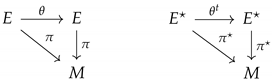
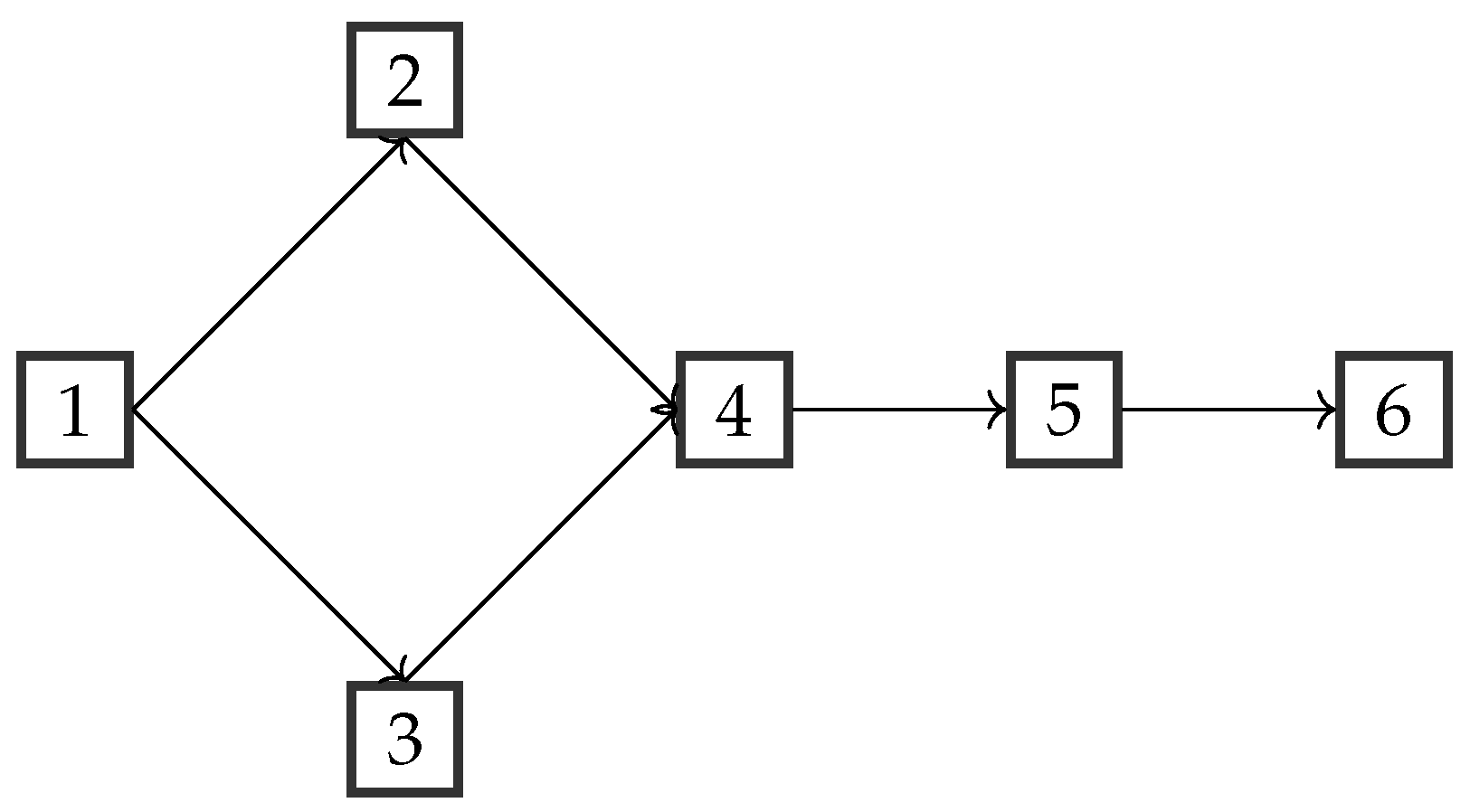
A reading diagram indicating dependencies between sections is provided in Figure 1.

Figure 1. Reading diagram.

2. The Gauge Equation

Let $E\stackrel{\pi }{⟶}M$ be a vector bundle. A Koszul connection ∇ is an $\mathbb{R}$-linear mapping [4]

$$\nabla :\Gamma \left(E\right)\to \Gamma \left(T^{★}M\otimes E\right)$$

(1)

such that ${\nabla }_{X}fs=df\otimes s+f{\nabla }_{X}s$ for any $f\in C^{\infty }\left(M\right)$. Let $E^{★}\stackrel{{\pi }^{★}}{⟶}M$ be the bundle obtained by dualizing E fiberwise. A section $\theta \in \Gamma \left(E^{*}\otimes E\right)$, that is, a $(1,1)$-tensor, defines two bundle morphisms:

(2)

where ${\theta }^t$ is such that $X\in T_{p}M,\xi \in T_p^{★}M$ for any $p\in M$:

$$\left({\theta }_p^t\xi \right)\left(X\right)=\xi \left({\theta }_{p}X\right).$$

(3)

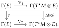
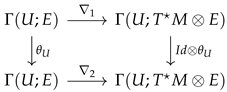
Definition 1.

Let $\left({\nabla }_1,{\nabla }_2\right)$ be a couple of Koszul connections. A $(1,1)$-tensor θ is said to be a solution of the gauge equation if, for any $s\in \Gamma \left(E\right)$,

$${\nabla }_2\theta s=\theta {\nabla }_{1}s,$$

(4)

or equivalently if the next diagram commutes:

(5)

Definition 1 can be made local, giving rise to the following diagrams:

(6)

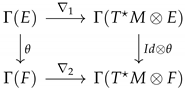
with U being an open subset of M and ${\theta }_U\in \Gamma \left(U;E^{★}\otimes E\right).$ The above definitions can be generalized to arbitrary vector bundles over M, giving rise to a category $\mathcal{GC}$ whose objects are couples $(E,\nabla )$, with E being a vector bundle on M, ∇ a Koszul connection on E, and morphisms being bundle morphisms $\theta :E\to F$ such that $(E,{\nabla }_1)\to (F,{\nabla }_2)$ if the diagram

(7)

commutes.

Definition 2.

Let be ∇ be an affine connection. Its dual is the affine connection

$${\nabla }^{★}:\Gamma \left(E^{★}\right)\to \Gamma \left(T^{★}M\otimes E^{★}\right)$$

(8)

defined by the relation

$$\left({\nabla }^{★}\xi \right)\left(s\right)=d\left(\xi \left(s\right)\right)-\xi \left(\nabla s\right).$$

(9)

Proposition 1.

If θ is a solution of the gauge equation with connections $\left({\nabla }_1,{\nabla }_2\right)$, then ${\theta }^{★}$ is a solution of the gauge equation with connections $\left({\nabla }_2^{★},{\nabla }_1^{★}\right)$.

Proof. 

For $s\in \Gamma \left(E\right),\xi \in \Gamma \left(E^{★}\right)$,

$$\begin{array}{cc}\hfill \left({\nabla }_2^{★}\left({\theta }^{★}\xi \right)\right)\left(s\right)& =\left({\theta }^{★}\xi \right)\left(s\right)-\left({\theta }^{★}\xi \right){\nabla }_{2}s=\xi \left(\theta s\right)-\xi \left(\theta {\nabla }_{2}s\right)\hfill \end{array}$$

(10)

$$\begin{array}{cc}\hfill \hspace{1em}& =\xi \left(\theta s\right)-\xi \left({\nabla }_1\theta s\right)=\left({\theta }^{★}{\nabla }_1^{★}\xi \right)\left(s\right).\hfill \end{array}$$

(11)

□

Given a couple of connections $\left({\nabla }_1,{\nabla }_2\right)$, the difference $D_{1,2}={\nabla }_1-{\nabla }_2$ is a section of $\Gamma \left(T{M}^{★}\otimes T{M}^{★}\otimes E\right).$ Using this, the gauge equation in Definition (1) can rewritten as

$${\nabla }_2\theta -\theta {\nabla }_2+D_{1,2}\theta =0.$$

(12)

Considering $\theta$ as an O-form with values in $E^{★}\otimes E$, Equation (12) may be rewritten as

$$d^{{\nabla }_2}\theta +D_{1,2}\theta =0,$$

(13)

where $d^{{\nabla }_2}$ is the exterior covariant derivative associated with the connection ${\nabla }_2.$

When ${\nabla }_2$ is flat, $d^{{\nabla }_2}{d}^{{\nabla }_2}=0$. Thus,

$$d^{{\nabla }_2}\left(D_{1,2}\theta \right)=0.$$

(14)

Recalling that the Gauge group $\mathcal{G}\left(E\right)$ is the set of bundle isomorphisms

(15)

then, given a connection ∇, $U\nabla U^{-1}$ is also a connection.

Proposition 2.

Let the triple $\left({\nabla }_1,{\nabla }_2,\theta \right)$ be a solution of the gauge equation ${\nabla }_1\theta =\theta {\nabla }_2.$ For any couple $(U,V)$ in $\mathcal{G}\left(E\right)$, the triple

$$\left(U{\nabla }_1{U}^{-1},U\theta V^{-1},V{\nabla }_2{V}^{-1}\right)$$

is a solution of a gauge equation.

Proof. 

Starting with ${\nabla }_1\theta =\theta {\nabla }_2$,

$$U^{-1}U{\nabla }_1{U}^{-1}U\theta V^{-1}V=U^{-1}U\theta V^{-1}V{\nabla }_2{V}^{-1}V.$$

(16)

Composing by U to the left and $V^{-1}$ to the right yields the result. □

Proposition 2 indicates that the existence of a solution does not depend on a particular choice of frame–coframe to represent it. Furthermore, locally, it is always possible to assume a $\theta$ of the form

$$\theta =\left(\begin{array}{cc}\mathrm{Id}& 0\\ 0& 0\end{array}\right),$$

(17)

as a pair $U,V$ such that $U\theta V^{-1}$ has the reduced form of Equation (17) exists by a standard linear algebra argument. Global reduction is not possible, however, as transition functions generally do not preserve the diagonal structure. Let $\tilde{E}$ be the bundle $E\oplus E^{★}$. The bilinear form

$$B:\left(X+\alpha ,Y+\beta \right)\in {\tilde{E}}^2\to \beta \left(X\right)+\alpha \left(Y\right)$$

(18)

is non-degenerate, that is,

$$\forall Y+\beta \in \tilde{E}B\left(X+\alpha ,Y+\beta \right)=0\Rightarrow X+\alpha =0.$$

(19)

Proposition 3.

A $(1,1)$-tensor θ on E satisfies the gauge equation for a couple of connections $\left({\nabla }_1,{\nabla }_2\right)$ if and only the bilinear form

$$B_{\theta }:\left(X+\alpha ,Y+\beta \right)\to B\left(X+\alpha ,\theta Y+{\theta }^{★}Y\right)$$

(20)

is parallel with respect to the connection $\tilde{\nabla }={\nabla }_2\oplus {\nabla }_1^{★}.$

Proof. 

By definition,

$$B\left(X+\alpha ,\theta Y+{\theta }^{★}Y\right)=\alpha \left(\theta Y\right)+{\theta }^{★}\beta \left(X\right).$$

(21)

Taking the differential yields

$$\begin{array}{cc}\hfill d\left(\alpha \left(\theta Y\right)\right)& =\left({\nabla }_1^{★}\alpha \right)\left(\theta Y\right)+\alpha \left({\nabla }_1\theta Y\right)=\left({\theta }^{★}‘{\nabla }_1★\alpha \right)\left(Y\right)+\alpha \left(\theta {\nabla }_{2}Y\right)\hfill \end{array}$$

(22)

$$\begin{array}{cc}\hfill & =\left({\nabla }_2^{★}{\theta }^{★}\alpha \right)\left(Y\right)+\alpha \left({\nabla }_1\theta Y\right)\hfill \end{array}$$

(23)

and symmetrically

$$\begin{array}{cc}\hfill d\left(\left({\theta }^{★}\beta \right)\left(X\right)\right)& =d\left(\beta \left)\right(\theta X)\right)\hfill \end{array}$$

(24)

$$\begin{array}{cc}\hfill & =\left({\nabla }_2^{★}{\theta }^{★}\beta \right)\left(X\right)+\beta \left({\nabla }_1\theta X\right).\hfill \end{array}$$

(25)

Now,

$$\begin{array}{cc}\hfill & \widetilde{B_{\theta }}\left(X+\alpha ,Y+\beta \right)=\hfill \end{array}$$

(26)

$$\begin{array}{cc}\hfill & d{B}_{\theta }\left(X+\alpha ,Y+\beta \right)-B_{\theta }\left(\tilde{\nabla }(X+\alpha ),Y+\beta \right)-B_{\theta }\left(X+\alpha ,\tilde{\nabla }(Y+\beta )\right)=\hfill \end{array}$$

(27)

$$\begin{array}{cc}\hfill & =d{B}_{\theta }\left(X+\alpha ,Y+\beta \right)-\beta \left({\nabla }_1\theta X\right)+\left({\nabla }_2^{★}{\theta }^{★}\alpha \right)\left(Y\right)-\alpha \left({\nabla }_1\theta X\right)+\left({\nabla }_2^{★}{\theta }^{★}\right)\beta \left(X\right)=0.\hfill \end{array}$$

(28)

Conversely, if $B_{\theta }$ is $\tilde{\nabla }$-parallel, then for any couple $(X+\alpha ,Y+\beta )$,

$$\alpha \left(\left({\nabla }_1\theta -\theta {\nabla }_2\right)Y\right)+\beta \left(\left({\nabla }_1\theta -\theta {\nabla }_2\right)X\right)=0.$$

(29)

Taking, $\alpha =0$ for example, with $\beta$ being arbitrary, we have

$$\left({\nabla }_1\theta -\theta {\nabla }_2\right)X=0,$$

(30)

proving that the couple $\left({\theta }_1,{\theta }_2\right)$ satisfies the gauge equation. □

The corollary below then immediately follows.

Corollary 1.

The kernel of $\tilde{\theta }=\theta \oplus {\theta }^{*}$ is $\tilde{\nabla }$-invariant; hence, the kernel of θ (resp. ${\theta }^{★}$) is ${\nabla }_2$ (resp. ${\nabla }_1^{★}$) invariant.

Proof. 

As the kernel of B is $\left\{0\right\}$, if

$$\forall Y+\beta \in \tilde{E},B_{\theta }\left(X+\alpha ,Y+\beta \right)=B(\theta X+{\theta }^{★}\alpha ,Y+\beta )=0,$$

(31)

then $\theta X+{\theta }^{★}\alpha =0$ and $X+\alpha \in ker\tilde{\theta }.$ Given a basis of $ker\tilde{\theta }$ at a point $p\in M$ and subjecting it to parallel transport by $\tilde{\nabla }$ yields another basis of $ker\tilde{\theta }$ at an arbitrary point $q\in M$; hence, the claim is sustained. □

Remark 1.

Corollary 1 implies by parallel transport that the dimension of the kernel of θ (resp. ${\theta }^{★}$) is a constant; hence, the rank of θ (resp. ${\theta }^{★}$) is also a constant.

Remark 2.

The kernel of ${\theta }^{★}$ is the set of differential forms vanishing on the image of $\theta .$ Thus, knowledge of the kernel of $B_{\theta }$ completely characterizes $ker\theta$ and $\mathsf{i}\mathsf{m}\theta .$ In particular, θ has constant rank.

When there exists a Riemannian metric on the manifold M, the gauge equation can be specialized to pairs of connections on $TM$ related by duality.

Definition 3.

Let ∇ be an affine connection. Its conjugate with respect to g (often referred to as the dual connection) is the connection ${\nabla }^{+}$, defined by the relation

$$\forall Z\in TM,\forall r,s\in \Gamma \left(TM\right),Z\left(g(r,s)\right)=g\left({\nabla }_{Z}r,s\right)+g\left(r,{\nabla }_Z^{+}s\right).$$

(32)

Remark 3.

The most common notation for the conjugate connection is ${\nabla }^{★}.$ In the present text, we adopt ${\nabla }^{+}$ to distinguish it from the connection on $E^{★}.$

Definition 4.

Let θ be a bundle morphism on $TM.$ Its conjugate, denoted ${\theta }^{+}$, is the bundle morphism defined by

$$\forall X,Y\in TM,g\left(\theta X,Y\right)=g\left(X,{\theta }^{+}Y\right).$$

(33)

Proposition 4.

If $U:TM\to TM$ is a unitary bundle isomorphism, that is, if

$$\forall X,Y\in TM,g\left(UX,UY\right)=g(X,Y),$$

then $U^{-1}=U^{+}.$

Proposition 5.

Let ∇ be a connection and let U be a unitary bundle isomorphism. Then,

$${\left(U\nabla U^{+}\right)}^{+}=U{\nabla }^{+}{U}^{+}.$$

(34)

Proof. 

If U is unitary, so is $U^{+}.$ Let $Z\in TM,r,sin\Gamma \left(TM\right)$; then,

$$\begin{array}{cc}\hfill Z\left(g(r,s)\right)& =Z\left(g(U^{+}r,U^{+}s)\right)\hfill \end{array}$$

(35)

$$\begin{array}{cc}\hfill & =g\left({\nabla }_Z{U}^{+}r,u^{+}s\right)+g\left(U^{+}r,{\nabla }_Z^{+}s\right)\hfill \end{array}$$

(36)

$$\begin{array}{cc}\hfill & =g\left(U{\nabla }_Z{U}^{+}r,s\right)+g\left(r,U{\nabla }_Z^{+}{U}^{+}s\right)\hfill \end{array}$$

(37)

and the claim follows. □

Proposition 6.

If the triple $\left(\nabla ,{\nabla }^{+},\theta \right)$ satisfies the gauge equation $\nabla \theta =\theta {\nabla }^{+}$, so does $\left(U\nabla ,U^{+},U{\nabla }^{+}{U}^{+},U^{+}\theta U\right)$ for any unitary isomorphism $U.$

Remark 4.

If θ is normal, that is, if $\left[\theta ,{\theta }^{+}\right]=0$, and if the triple $\left(\nabla ,{\nabla }^{+},\theta \right)$ satisfies the gauge equation $\nabla \theta =\theta {\nabla }^{+}$, then locally there exists a unitary isomorphism U such that $U^{+}\theta U$ is diagonal and $\left(U\nabla ,U^{+},U{\nabla }^{+}{U}^{+},U^{+}\theta U\right)$ satisfies a gauge equation. Again, this is a well known fact from linear algebra, as θ is locally diagonalizable in an orthonormal frame. As in the case of Equation (17), this is generally not true globally.

Proposition 7.

Using the musical isomorphisms $\begin{array}{c}TM\underset{♯}{\overset{♭}{\rightleftarrows }}{T}^{★}M\end{array}$ we have

$$\forall X\in TM,\alpha \in T^{★}M\left({\nabla }_X^{+}{\alpha }^{♯}\right)={\left({\nabla }_X\alpha \right)}^{♯}.$$

Proof. 

For any $X,Y,Z\in TM$,

$$Z\left(g(X,Y)\right)=g\left({\nabla }_{Z}X,Y\right)+g\left(X,{\nabla }_Z^{+}Y\right).$$

Passing to forms, for any $Z\in TM$ $\alpha in{T}^{★}M$, $X\in TM$,

$$Z\left(g(X,{\alpha }^{♯})\right)=g\left({\nabla }_{Z}X,{\alpha }^{♯}\right)+g\left(X,{\nabla }_Z^{+}{\alpha }^{♯}\right).$$

Now,

$$\begin{array}{cc}\hfill Z\left(g(X,{\alpha }^{♯})\right)& =Z\left(\alpha \left(X\right)\right)=\left({\nabla }^{★}\alpha \right)\left(X\right)+\alpha \left({\nabla }_{Z}X\right)\hfill \\ & g\left(X,{\left({\nabla }^{★}\alpha \right)}^{♯}\right)+g\left({\nabla }_{Z}X,{\alpha }^{♯}\right)\hfill \end{array}$$

and the claim follows from identification. □

Proposition 8.

Let the triple $\left(\nabla ,{\nabla }^{+},\theta \right)$ satisfy the gauge equation $\nabla \theta =\theta {\nabla }^{+}.$ Then, the tensor

$$g_{\theta }:(X,Y)\mapsto g\left(\theta X,Y\right)$$

(38)

is ∇ parallel.

Proof. 

Tensor $B_{\theta }$ in Proposition 3 can be written using the metric as follows:

$$\begin{array}{cc}\hfill B_{\theta }\left(X+\alpha ,Y+\beta \right)& =\beta \left(\theta X\right)+\alpha \left(\theta Y\right)\hfill \end{array}$$

(39)

$$\begin{array}{cc}\hfill & =g\left(\theta X,{\beta }^{♯}\right)+g\left({\alpha }^{♯},\theta Y\right).\hfill \end{array}$$

(40)

Because $B_{\theta }$ is $\tilde{\nabla }$-parallel, the proposition follows. □

Remark 5.

Defining a metric $g^{★}$ on $T^{★}M$ by

$$\forall \alpha ,\beta \in T^{★}M,g^{★}(\alpha ,\beta )=g\left({\alpha }^{♯},{\beta }^{♯}\right),$$

(41)

the proof of Proposition 8 also shows that the tensor

$$g_{\theta }^{★}:(\alpha ,\beta )\mapsto g^{★}\left({\theta }^{★}\alpha ,\beta \right)$$

is ${\nabla }^{★}$-parallel.

Proposition 8 has the important consequence that $TM$ can be split in two ways:

$$TM=ker\theta \oplus \mathsf{im}\theta ,TM=ker{\theta }^{+}\oplus \mathsf{im}{\theta }^{+}.$$

(42)

It is clear from Proposition 8 that if $\theta$ is symmetric, that is, if $\theta ={\theta }^{+}$, then the tensor

$$(X,Y)\mapsto \frac{1}{2}g\left(\theta X,Y\right)+g\left(\theta X,Y\right)$$

(43)

is ∇-parallel. When $\theta$ is skew-symmetric, i.e., $\theta =-{\theta }^{+}$, the same is true for

$$(X,Y)\mapsto \frac{1}{2}g\left(\theta X,Y\right)-g\left(\theta X,Y\right).$$

(44)

As in Equation (7), there is a category such that morphisms represent gauge equation solutions. The situation is nevertheless a little bit more complicated, as the dimension of the vector bundle may not agree. We recall the following well-known definition.

Definition 5.

Let $E\to M$ be a vector bundle. A pseudo-Riemannian metric on E is a smooth bilinear $C^{\infty }\left(M\right)$-mapping $g_E:\Gamma \left(E\right)\times \Gamma \left(E\right)\to C^{\infty }\left(M\right)$ such that:

• $\forall s,s^{\prime }\in \Gamma \left(E\right),g_E(s,s^{\prime })=g_E(s^{\prime },s)$;
• There exists an isomorphism ^♭: $\Gamma \left(E\right)\to \Gamma \left(E^{★}\right)$ such that, for any $s,s^{\prime }\in \Gamma \left(E\right)$,

  $$s^{♭}\left(s^{\prime }\right)=g_E(s,s^{\prime }).$$

A pseudo-Riemannian metric is Riemannian if $g_E(s,s)>0$ for any $s\ne 0$ in $\Gamma \left(E\right).$

Definition 6.

Let $E,F$ be two vector bundles on M equipped with respective Riemannian metrics $g_E,g_F.$ A partial isometry from E to F is a bundle morphism U such that the following diagram commutes.

(45)

Remark 6.

Definition 6 is equivalent to the fact that, for any $s,s^{\prime }\in \Gamma \left(E\right)$, we have

$$g_F\left(Us,U{s}^{\prime }\right)=g_E\left(s,s^{\prime }\right).$$

Definition 7.

Let $U:E\to F$ be a partial isometry and let ${\nabla }_2$ be a Koszul connection on F. Its dual ${\nabla }_2^{+}$ is the connection on E defined by the relation

$$U{\nabla }_2^{+}={\nabla }_{2}U.$$

(46)

Definition 8.

The category $\mathcal{GU}$ has objects $(E,\nabla )$, with ∇ a Koszul connection on E and morphisms $(U,\theta ):(E,{\nabla }_1)\to (F,{\nabla }_2)$, where $U:E\to F$ is a partial isometry, $\theta :E\to F$ is a bundle morphism, and ${\nabla }_1={\nabla }_2^{+},{\nabla }_2\theta =\theta {\nabla }_1.$

The next two examples illustrate the gauge equation in simple situations.

Example 1.

Take $M={\mathbb{R}}^2$ and consider the following symplectic 2-form:

$$\omega :(x,y)\mapsto expxdx\wedge dy.$$

(47)

Let ∇ be a Koszul connection such that $\nabla \omega =0$, let g be an arbitrary Riemannian metric on ${\mathbb{R}}^2$, and let ${\nabla }^{+}$ be the dual of ∇ with respect to g; finally, let θ be the unique $(1,1)$-tensor such that, for all vector fields $X,Y$,

$$\omega (X,Y)=g(\theta X,Y).$$

(48)

Then,

$${\nabla }_X^{+}\theta Y=\theta {\nabla }_{X}Y.$$

(49)

Example 2.

Take $M={\mathbb{S}}^3$, with ∇ as a torsion-less connection and g as a Riemannian metric. Any solution θ to the gauge equation

$${\nabla }_X^{+}\theta Y=\theta {\nabla }_{X}Y$$

(50)

is either 0 or invertible.

3. KV Cohomology

The co-chain complex of Koszul–Vinbeg algebras may be introduced in any of the following three ways [5,6]:

• 1: From the point of view of the tensor calculus, i.e., the raw formula.
• 2: From the point of view of the theory of categories, i.e., simplicial objects.
• 3: From the point of view of the anomalies, viz. the calculation rules.

In this work, we take into account forthcoming applications with interests in the relationship between information geometry and differential topology.

3.1. Koszul–Vinberg Algebras

We first recall some useful basic definitions.

Definition 9.

A real Koszul–Vinberg algebra is a real vector space A endowed with a product

$$A\times A\ni (a,b)\to ab\in A$$

subject the following identity:

$$(a,b,c)=(b,a,c)$$

(51)

where

$$(a,b,c)=\left(ab\right)c-a\left(bc\right).$$

(52)

Examples include:

(a)

Associative algebras are Koszul–Vinberg algebras.

(b)

The vector of vector fields on a smooth manifold M endowed with a symmetric flat Koszul connection ∇.

3.2. KV Modules of Koszul–Vinberg Algebras

Definition 10.

A real left module of a real Koszul–Vingerg algebra A is a real vector space V endowed with a bilinear mapping

$$A\times V\ni (a,v)\to a.v\in V$$

which satisfies the following identity:

$$(a,a^{\prime },v)=(a^{\prime },a,v)$$

(53)

where

$$(a,a^{\prime },v)=\left(a{a}^{\prime }\right).v-a.(a^{\prime }.v).$$

(54)

In this paper, we are dealing with Koszul–Vinberg algebra of vector fields $\mathcal{X}\left(M\right)$ on a differentiable manifold M endowed with a Koszul connection ∇ for which both the curvature tensor $R^{\nabla }$ and the torsion tensor $T^{\nabla }$ vanish identically. We write

$$A:=\left(\mathcal{X}\right(M),\nabla ).$$

The product on A is defined as follows:

$$a.a^{\prime }={\nabla }_a{a}^{\prime }.$$

(55)

Here, $\mathcal{X}\left(M\right)$ is obviously a left Koszul–Vinberg module of $A.$

Moreover, the space of smooth functions $C^{\infty }\left(M\right)$ is a left Koszul–Vinberg module of A under the left action

$$A\times C^{\infty }\left(M\right)\ni (a,f)\to df\left(a\right)\in C^{\infty }\left(M\right).$$

(56)

3.3. Vector Co-Chain Complexes

Given a Koszul–Vinberg algebra A, the following two cochain complexes of A with coefficients in V are associated with any left module module V. One is denoted by $C_{KV}(A,V)$ and is named the KV complex; the other is denoted $C_{\tau }(A,V)$, and is named the total KV complex. We remind readers of the definition of these complexes, and point out some domains of their efficiency.

3.3.1. $C_{KV}(A,V)$ Complex

We set

$$J\left(V\right)=\left\{v\in Vs.t.(a,a^{\prime },v)=0\forall (a,a^{\prime })\subset A\right\}.$$

(57)

Given

$$\xi =a_1\otimes \cdots \otimes a_{q+1}\in A^{\otimes q+1},$$

(58)

we set

$$\begin{array}{cc}\hfill & {\partial }_i\xi =\cdots \otimes {\widehat{a}}_i\otimes \cdots \hfill \\ \hfill & a.\xi ={\Sigma }_i\cdots \otimes a.a_i\otimes \cdots \hfill \end{array}$$

(59)

The vector space $C_{KV}(A,V)$ is $\mathbb{Z}$-graded by the homogeneous subspaces $C_{KV}^q$, which are defined as follows:

$$\left\{\begin{array}{cc}\hfill & C_{KV}^q=0\mathrm{if}q<0\hfill \\ \hfill & C_{KV}^0=J\left(V\right)\hfill \\ \hfill & C_{KV}^q=Hom(A^{\otimes q},V),q>0.\hfill \end{array}\right.$$

(60)

The operator $\delta$,

$$C_{KV}^q\ni f\to \delta .f{C}_{KV}^{q+1},$$

is defined by the relation

$$\delta .v\left(a\right)=a.v(a,v)\in A\times J\left(V\right).$$

(61)

Let $f\in C_{KV}^q$ and $\xi =a_1\otimes \cdots \otimes a_{q+1}$; then,

$$\delta .f\left(\xi \right)={\Sigma }_1^q{(-1)}^{i-1}[a_i.f\left({\partial }_i\xi \right)-f(X_i.{\partial }_i\xi )].$$

(62)

The q-th cohomology space is denoted by

$$H_{KV}^q(A,V)=\frac{ker(\delta :C_{KV}^q\to C_{KV}^{q+1})}{\delta \left(C_{KV}^{q-1}\right)}.$$

(63)

Remark 7.

The cohomology of Equation (63) is the solution to a conjecture of Gerstenhaber for the deformations of hyperbolic structures in the sense of Koszul [7,8], claiming that “Every restricted theory of deformation generates its proper theory of cohomology” [9].

This cohomology characterizes the equivalence between extensions of Koszul–Vinberg algebras by Koszul–Vinberg modules. Let $Ext(A,V)$ be the set of equivalence classes of extensions of A by V; then,

$$Ext(A,V)=H_{KV}^2(A,V).$$

(64)

Remark 8.

In the category of modules of associative algebras (resp. the category of modules of Lie algebras), the second Hochschild space $H{H}^2(-,-)$ (resp. the second Chevalley–Eilbenberg space $H_{CE}^2(-,-)$) plays a similar role.

3.3.2. Total KV Complex $C_{\tau }(A,V)$

The co-chain complex $C_{\tau }(A,V)$ is $\mathbb{Z}$-graded by the homogeneous subspaces $C_{\tau }^q(A,V)$, defined as follows:

$$\left\{\begin{array}{cc}\hfill & C_{\tau }^q=0\mathrm{if}q<0\hfill \\ \hfill & C_{\tau }^0=V\hfill \\ \hfill & C_{\tau }^q=Hom(A^{\otimes q},V)\mathrm{if}q>0.\hfill \end{array}\right.$$

(65)

Keeping the notation from Section 3.3.1, the operator ${\delta }_{\tau }$ is defined as follows:

$$\left\{\begin{array}{cc}\hfill & {\delta }_{\tau }v\left(a\right)=a.v\mathrm{if}v\in C^0\hfill \\ \hfill & {\delta }_{\tau }f\left(\xi \right)={\Sigma }_1^{q+1}{(-1)}^{i+1}[a_i.f\left({\partial }_i\xi \right)-f(a_i.\partial \xi )]\mathrm{if}f\in C_{\tau }^q.\hfill \end{array}\right.$$

(66)

The q-th cohomology space of the total complex is then

$$H_{\tau }^q(A,V)=\frac{Ker({\delta }_{\tau }:C_{\tau }^q\to C_{\tau }^{q+1})}{{\delta }_{\tau }\left(C_{\tau }^{q-1}\right)}.$$

(67)

3.4. Scalar Complexes $C_{KV}(A,R)$ and $C_{\tau }(A,R)$

Setting $A=\left(\mathcal{X}\right(M),\nabla )$, $V=C^{\infty }\left(M\right)$, the scalar co-chain complex $C_{KV}(A,R)$ is defined as follows:

$$\left\{\begin{array}{cc}\hfill & C_{KV}^q(A,R)=0\mathrm{if}q<0\hfill \\ \hfill & C_{KV}^0(A,R)=J\left(C^{\infty }\left(M\right)\right),\mathrm{the}\mathrm{space}\mathrm{of}\mathrm{affine}\mathrm{functions}\hfill \\ \hfill & C_{KV}^q(A,R)=Hom(A^{\otimes q},C^{\infty }\left(R\right))\mathrm{if}q>0.\hfill \end{array}\right.$$

(68)

The total scalar cohomology $C_{\tau }(A,R)$ is defined by

$$\left\{\begin{array}{cc}\hfill & C_{\tau }^q(A,R)=0\mathrm{if}q<0\hfill \\ \hfill & C_{\tau }^0(A,R)=C^{\infty }\left(M\right),\mathrm{if}q>0\hfill \\ \hfill & C_{\tau }^q(A,R)=Hom(A^{\otimes q},C^{\infty }\left(M\right))\mathrm{if}q>0.\hfill \end{array}\right.$$

(69)

3.5. Links with the de Rham Complex

In this section, we highlight an important inclusion relation of the de Rham complex into the KV complex, yielding a long exact sequence in cohomology.

We consider the real de Rham complex which is

$$\Omega \left(M\right)=\oplus {\Omega }^q(M,R),{\Omega }^q(A,R)=Hom({\Lambda }^{q}A,C^{\infty }\left(M\right)).$$

(70)

Its differential $d:{\Omega }^q\left(M\right)\to {\Omega }^{q+1}\left(M\right)$ is defined as follows:

$$d\omega (a_0\wedge \cdots \wedge a_q={\Sigma }_0^q{(-1)}^i{a}_i.\omega (\cdots \wedge {\widehat{a}}_i\wedge \cdots )+{\Sigma }_{i<j}{(-1)}^{i+j}\omega ([a_i,a_j]\wedge \cdots \wedge {\widehat{a}}_i\wedge \cdots {\widehat{a}}_j\wedge \cdots ).$$

(71)

The inclusion map ${\Omega }^q\left(M\right)\subset C_{\tau }^q(A,R)$ yields the following cochain complex injective morphism:

$$(\Omega \left(M\right),d)\to (C_{\tau }(A,R),{\delta }_{\tau }).$$

(72)

Denoting the quotient complex by

$$H(Q,d)=\frac{(C_{\tau }(A,R),\delta )}{(\Omega (M),d)},$$

(73)

there is a short exact sequence of cochain complexes:

$$\begin{array}{ccccc}\hfill O⟶& (\Omega (M),d)⟶& (C_{\tau }(A,R),\delta \tau )⟶\hfill & (Q,d)⟶& 0.\end{array}$$

(74)

Equation (74) gives rise to a long cohomology exact sequence:

$$\begin{array}{cccccc}\hfill \dots ⟶& H_{dR}^q(M,R)⟶& H_{\tau }^q(A,R)⟶\hfill & H^q\left(Q\right)⟶& H_{dR}^{q+1}(M,R)⟶& \dots \end{array}$$

(75)

3.6. Tensor Product of Two KV Complexes

In the category of statistical geometry, we are interested in spectral sequences which arise from particular double complexes. We consider two Koszul–Vinberg algebras, A and $A^{★}$. Let W be a left KV module of the both A and $A^{★}$. From this situation, the following four cochain complexes arise:

$$\begin{array}{cc}\hfill & \left(I\right):C_{KV}(A,W),\hfill \\ \hfill & \left(II\right):C_{KV}(A^{★},W),\hfill \\ \hfill & \left(III\right):C_{\tau }(A,W),\hfill \\ \hfill & \left(IV\right):C_{\tau }(A^{★},W).\hfill \end{array}$$

(76)

Let us consider the bi-graded vector space $C\left(W\right)$:

$$C^{q,p}=C_{\tau }^q(A,W)\otimes C_{\tau }^p(A^{★},W).$$

(77)

We set $C^m={\Sigma }_{q+p=m}{C}^{q,p}$. Given $\alpha \otimes \beta \in C^{q,p}$, we let

$$\delta (\alpha \otimes \beta )=[{\delta }_{\tau }\alpha \otimes \beta +{(-1)}^q\alpha \otimes {\delta }_{\tau }\beta ]\in C^{q+1,p}\oplus C^{q,p+1}.$$

(78)

It is clear that d is a differential $\delta \circ \delta =0.$

The cohomology space $H^{q,p}$ is defined as follows:

$$H^{q,p}=\frac{ker(\delta :C^{q,p}\to C^{q+1,p}\oplus C^{q,p+1})}{im\left(\delta \right)\cap C^{q,p}}.$$

(79)

4. Statistical Manifolds

We recall that a statistical manifold is a quadruple $(M,g,\nabla ,\nabla )$ such that ∇ and ${\nabla }^{+}$ are dual connections with respect to the metric g which are both torsion-free. These structures are of the utmost importance in information geometry [10,11], and are named after their appearance in statistical problems [12].

In Hessian statistical manifolds, solutions of gauge equations give rise to statistical 2-webs, i.e., webs bearing the structure of a statistical manifold. These 2-webs are canonically associated with tensor products of co-chain complexes, the cohomology of which can be calculated with spectral sequences. Situations (I), (II), (III), and (IV) in Equation (76) arise in any Hessian manifold $(M,g,\nabla )$.

In this section, we retain the notation from Section 2 and Section 3 and fix a statistical manifold $(M,g,\nabla ,{\nabla }^{+}).$

Let $\theta$ be a solution of the gauge equation ${\nabla }^{+}\theta =\theta \nabla .$ We define another pair of solutions $(\Theta ,{\Theta }^{★})$ by the identities

$$\begin{array}{cc}\hfill & 2g(\Theta (X),Y)=g\left(\theta \right(X),Y)+g(X,\theta (Y\left)\right),\hfill \\ \hfill & 2g({\Theta }^{★}\left(X\right),Y)=g(\theta \left(X\right),Y)-g(X,\theta \left(Y\right)).\hfill \end{array}$$

(80)

All of the four distributions $\left\{Ker(\Theta ),Im(\Theta ),Ker\left({\Theta }^{★}\right),Im\left({\Theta }^{★}\right)\right\}$ are regular and are in involution. Furthermore, we have the following 2-webs:

$$\left\{\begin{array}{cc}\hfill & TM=K\oplus I\hfill \\ \hfill & TM=K^{★}\oplus I^{★}\hfill \\ \hfill & K^{★}=ker\left({\Theta }^{★}\right)\hfill \\ \hfill & I^{★}=im\left({\Theta }^{★}\right)\hfill \end{array}\right.$$

(81)

where $K=ker(\Theta ),I=im(\Theta ).$

These distributions are parallel with respect to ∇, ${\nabla }^{+}$, as indicated by the identities

$$\begin{array}{cc}\hfill & {\nabla }_{X}K=K,\hfill \\ \hfill & {\nabla }_X{K}^{★}=K^{★},\hfill \\ \hfill & {\nabla }_X^{+}I=I,\hfill \\ \hfill & {\nabla }_X^{+}{I}^{★}=I^{★}.\hfill \end{array}$$

(82)

Here, the foliations $K,I$ are Riemannian [13,14,15].

Remark 9.

If either $(M,g,\nabla )$ or $(M,g,{\nabla }^{+})$ are Hessian manifolds, then K, $K^{★}$, I, and $I^{★}$ are Hessian foliations. Thus, any of the pairs $(K,I)$ and $(K^{★},I^{★})$ gives rise to a double co-chain complex as in Equation (79).

Any of the three distributions $ker\left(\theta \right)$, $ker(\Theta )$, and $ker\left({\Theta }^{★}\right)$ is of constant rank. The three ranks may be different.

Remark 10.

Note that a foliated manifold carries two other remarkable complexes in addition to its total de Rham complex, namely, the complex of foliated forms, and the complex of basic forms.

Assuming that $(M,g,\nabla ,{\nabla }^{+})$ is a Hessian statistical manifold, we may construct two Koszul–Vinberg algebras

$$A=(\mathcal{X},\nabla ),A^{★}=(\mathcal{X}\left(M\right),{\nabla }^{+}).$$

(83)

The two associated KV-complexes $C_{KV}(A,R)$ and $C_{\tau }(A^{★},\mathcal{X}\left(M\right))$ are of particular interest.

Proposition 9.

On the Hessian manifold $(M,g,\nabla )$, the Riemannian metric tensor g is a 1-cocycle of the scalar KV complex $(C_{KV}(A,R))$.

Corollary 2.

In order for $(M,g,\nabla )$ to be hyperbolic, it is necessary that $\left[g\right]=0$. It is also sufficient if M is compact.

The next proposition makes use of the vector total KV complex to obtain a cohomological obstruction for a section $\theta \in hom(TM,TM)$ to be a solution of the gauge equation.

Proposition 10.

The gauge equation ${\nabla }^{+}\varphi -\varphi \nabla =0$ is equivalent to the cohomology equation

$${\delta }_{\tau }\varphi =0.$$

(84)

Equation (84) is essentially Equation (14) rewritten; however, the vector KV complex is more tractable than the complex of $(T{M}^{★}\otimes TM)$-valued forms.

4.1. Tensor Products

For every non-negative integer q, the dual vector spaces $\Gamma \left(K^{\otimes q}\right)$ and of $\Gamma \left({\Lambda }^{q}K\right)$ are denoted by $C^q\left(K\right)$ and b ${\Omega }_K^q\left(M\right)$, respectively, and we set

$$C\left(K\right)={\oplus }_q{C}^q\left(K\right),{\Omega }_K\left(M\right)={\oplus }_q{\Omega }_K^q\left(M\right).$$

(85)

It makes sense to restrict the de Rham operation to ${\Omega }_K\left(M\right)$ in order to define a cochain complex

$$\begin{array}{ccccc}\hfill \dots ⟶& {\Omega }_K^{q-1}\left(M\right)⟶& {\Omega }_K^q\left(M\right)⟶\hfill & {\Omega }_K^{q+1}\left(M\right)⟶& \dots \end{array}$$

(86)

In any Hessian manifold, we may use Remark 9 and the operators ${\delta }_{KV}$, ${\delta }_{\tau }$ to write the KV cochain complexes $[C\left(K\right),{\delta }_{\tau }]$ and $[C\left(K\right),{\delta }_{\tau }]$ as follows:

$$[C\left(K\right),{\delta }_{KV}]:0\to J\left(C^{\infty }\left(M\right)\right)\to \cdots .\to C^{q-1}\left(K\right)\to C^q\left(K\right)\to C^{q+1}\left(K\right)\to$$

(87)

and

$$[C\left(K\right),{\delta }_{\tau }]:0\to C^{\infty }\left(M\right)\to \cdots \to C^{q-1}\left(K\right)\to C^q\left(K\right)\to C^{q+1}\left(K\right)\to$$

(88)

We note that the cochain Equation (88) is then nothing other than

$$\to C_{KV}^{q-1}(A_K,R)\to C_{KV}^q(A_K,R)\to C_{KV}^{q+1}(A_K,R)\to$$

(89)

where $A_K=\Gamma (K=ker(\Theta )).$

Remark 11.

Similar complexes are attached to the three other distributions (I, $K^{★}$, and $I^{★}$).

4.2. Double Complexes in a Hessian Manifold

Let $(M,g,\nabla ,{\nabla }^{+})$ be a Hessian statistical manifold. Two de Rham double complexes derive from the following 2-webs: $\Omega (K,I),\Omega (K^{★},I^{★}).$

To investigate the properties of $(g,\nabla ,{\nabla }^{+})$, we can use the two Koszul–Vinberg algebras $A=(\Gamma \left(TM\right),\nabla ),A^{★}=(\Gamma \left(TM\right),{\nabla }^{+})$ and the complexes

$$\begin{array}{cc}\hfill & C_{KV}(A,R),\hfill \\ \hfill & C_{KV}(A^{★},R),\hfill \\ \hfill & C_{\tau }(A,R),\hfill \\ \hfill & C_{\tau }(A^{★},R).\hfill \end{array}$$

(90)

Furthermore, we have the two double KV complexes

$$\begin{array}{cc}\hfill & C_{KV}(A,A^{★})={\oplus }_{q,p}{C}_{KV}^q(A,R)\otimes C_{KV}^p(A^{★},R),\hfill \\ \hfill & C_{\tau }(A,A^{★})=\oplus C_{\tau }^q(A,R)\otimes C_{\tau }^p(A^{★},R).\hfill \end{array}$$

(91)

These double complexes give rise to the total complexes $(C_{KV}\left(M\right),d_{KV}),(C_{\tau }\left(M\right),d_{\tau })$, with $C_{\tau }\left(M\right)={\oplus }_n{C}_{\tau }^n\left(M\right)$ and $C_{\tau }^n\left(M\right)={\oplus }_{[q+p=n]}{C}^q\tau (A,R)\otimes C_{\tau }^p(A^{★},R).$ The operator $d_{\tau }:C_{\tau }^n\left(M\right)\to C_{\tau }^{n+1}\left(M\right)$ is defined by the relation

$$d_{\tau }:u\otimes v\in C_{\tau }^q(A,R)\otimes C_{\tau }^p(A^{★},R)\mapsto {\delta }_{\tau }\left(u\right)\otimes v+{(-1)}^{q}u\otimes {\delta }_{\tau }\left(v\right).$$

(92)

Mutatis mutandis, $(C_{KV},d_{KV})$ is defined in the same way.

Let G be the group of symmetries of $(M,g,\nabla ,{\nabla }^{★})$; then, G is the following finite dimensional Lie group:

$$G=Isom(M,g)\cap Aff(M,\nabla ).$$

(93)

The cohomology spaces of the complexes which are introduced above are geometric invariants of G.

4.3. Gauge Equation and Homology Persistence

Before proceeding with cohomology calculations, in this section we introduce useful materials derived from persistent simplicial homologies which are related to the gauge equation.

Let $(M,g,\nabla ,{\nabla }^{+})$ be a statistical manifold and let $\theta$ be a solution of the gauge equation of $({\nabla }^{+},\nabla )$. According to the notation used in the preceding sections, $\theta$ gives rise to two 2-webs $(K,I),(K^{★},I^{★}).$ The foliation defined by $I^{★}$ is denoted by ${\mathcal{F}}_{\theta }$.

Let $r^{★}\left(\theta \right)$ be the rank of the distribution $I^{★}$. We set

$$r^{★}\left(M\right)=\underset{\theta }{max}\left\{r^{★}\left(\theta \right)\right\}.$$

(94)

Step 1.

We choose a ${\theta }_1$ such that $r^{★}\left({\theta }_1\right)=r^{★}\left(M\right)$ and fix a point $x\in M$. Let $F_1\left(x\right)$ be the leaf of ${\mathcal{F}}_{{\theta }_1}$ which contains x. The $r^{★}\left(M\right)$-dimensional submanifold

$$(F_1\left(x\right),g,{\nabla }^{+})\subset (M,g,{\nabla }^{+})$$

(95)

inherits the statistical structure (i.e., $g,\nabla ,{\nabla }^{+}$) from $M.$

Step 2.

We use the gauge equation of $F_x(g,{\nabla }^{+})$ to define $r^{★}\left(F_1\left(x\right)\right)$, obtaining the statistical submanifold

$$(F_2\left(x\right),g,{\nabla }^{+})\subset (F_1\left(x\right),g,{\nabla }^{+}).$$

(96)

Setting

$$(F_0,g,{\nabla }^{+})=(M,g,{\nabla }^{+}),$$

(97)

we can inductively construct the next statistical filtration:

$$SP\left(M\right):(F_q\left(x\right),g,{\nabla }^{+})\subset (F_{q+1}\left(x\right),g,{\nabla }^{+})\subset \cdots \subset (M,g,{\nabla }^{+}).$$

(98)

In addition, we consider the real singular chain complex of M:

$$Sing\left(M\right):\to C_{q+1}\left(M\right)\to C_q\left(M\right)\to C_{q-1}\left(M\right)\to$$

(99)

The topology persistence $\left(SP\right(M)$ yields the following homology persistence:

$$HP\left(M\right):\to Sing\left(F_{q+1}\left(x\right)\right)\to Sing\left(F_q\left(x\right)\right)\to Sing\left(F_{q-1}\left(x\right)\right)\to$$

(100)

5. Spectral Sequences

In this section, we briefly recall the definition of spectral sequences of co-chain complexes. A good recent reference on this subject is [16].

Definition 11.

A graded differential sheaf $\left(\mathcal{S},d\right)$ denotes a graded sheaf ${\left({\mathcal{S}}^p\right)}_{p\in \mathbb{Z}}$ together with a graded morphism $d:{\mathcal{S}}^p\to {\mathcal{S}}^{p+1}$ satisfying $d^2=0.$

Definition 12.

The derived cohomology sheaf indicates the graded sheaf $H$ ():

$$H^p\left(\mathcal{S}\right)=\frac{ker\{d^p:{\mathcal{S}}^p\to {\mathcal{S}}^{p+1}\}}{\mathsf{i}\mathsf{m}\{d^{p-1}:{\mathcal{S}}^{p-1}\to {\mathcal{S}}^p\}}.$$

(101)

Remark 12.

The derived cohomology sheaf is the sheafification of the local cohomology presheaf

$$U\mapsto H^p\left(\mathcal{S}\left(U\right)\right).$$

In the following, a ring R is fixed.

Definition 13.

A bi-graded module E over R is a double-indexed collection of R-modules $E^{p,q},p,q\in \mathbb{Z}.$

Definition 14.

Let E be a bi-graded module over R and let $r\in \mathbb{N}$; a differential over E of bi-degree $(r,1-r)$ is a double-indexed collection of R-morphisms $d:E^{p,q}\to E^{p+r,q+1-r}$ such that $d^2=0.$

Definition 15.

A differential bi-graded R-module is a couple $(E,d)$, with E being a bi-graded module, d a differential of bi-degree $(r,1-r)$, and r a fixed integer.

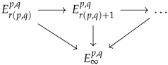
Definition 16.

A cohomology spectral sequence is a sequence of bi-graded differential modules $(E_r,d_r),r=1,2,\dots$, where $d_r$ has bi-degree $(r,1-r)$ and $E_{r+1}^{p,q}\sim H^{p,q}(E_r,d_r)$ for all $p,q,r$.

Remark 13.

A spectral sequence can be viewed as a successive approximation process; in most cases, $(E_2,d_2)$ is known and is the starting point of the sequence. Now, looking at stage n, that is, $(E_n,d_n)$, the defining property of the spectral sequence indicates that if $Z_n=ker{d}_n,B_n=\mathsf{i}\mathsf{m}{d}_{n-1}$, then, as a bi-graded module, $E_{n+1}\sim Z_n/B_n.$ Now, if ${\overline{Z}}_{n+1}=ker{d}_{n+1},{\overline{B}}_{n+1}=\mathsf{i}\mathsf{m}{d}_n$, there exist modules $Z_{n+1},B_{n+1}$ such that ${\overline{Z}}_{n+1}=Z_{n+1}/B_n$, ${\overline{B}}_{n+1}=B_{n+1}/B_n$. Thus, per Noether’s isomorphism, $Z_{n+1}/B_{n+1}={\overline{Z}}_{n+1}/{\overline{B}}_{n+1}.$ Furthermore, because $d_{n+1}$ is a differential, $\overline{B_{n+1}}\supset B_n,\overline{z_{n+1}}\subset Z_n$; hence, $B_n\subset B_{n+1}\subset Z_{n+1}\subset Z_n.$ Proceeding by recurrence, there exist limiting modules

$$B_{\infty }={\cup }_n{B}_n,Z_{\infty }={\cap }_n{Z}_n,$$

and the purpose of the spectral sequence is to obtain $Z_{\infty }/B_{\infty }.$

Definition 17.

A spectral sequence is said to converge if, for each couple of integers $(p,q)$, there exists an integer $r(p,q)$ such that all differentials $d_r:E_r^{p,q}\to E_{p+r,q+1-r}$ are 0 for $r\ge r(p,q).$

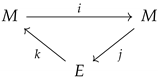
Proposition 11.

If a spectral sequence converges, then for any couple of integers $p,q$, the module $E_{\infty }^{p,q}$ is isomorphic to the direct limit of the following diagram.

(102)

Definition 18.

An exact couple is a pair of modules $M,E$ and morphisms $i,j,k$ fitting in the following exact diagram.

(103)

Proposition 12.

Given an exact couple as in Definition 18, E is differential module with differential $d=j\circ k$.

The next proposition can be found in [16,17].

Proposition 13.

Let $(M,E,i,j,k)$ be an exact couple. The derived couple $M_1=\mathsf{i}\mathsf{m}\left(i\right),E_1=H\left(E\right)$ is exact with morphisms

$$i_1{=i|}_{M_1},j_1=j\circ i+dE,k_1(e+dE)=k\left(e\right).$$

Passing to bi-graded modules and iterating the process defines a spectral sequence $(E_r,d_r)$, where $E_r$ is the r-th derived module of E and $d_r=j_r\circ k_r.$

Finally, still using [16], a filtered complex $F^p\mathcal{C}\subset F^{p+1}\mathcal{C}\subset \dots$ defines an exact couple by passing to cohomology; that is, starting with the short exact sequence

$$\begin{array}{ccccc}\hfill 0⟶& F^p\mathcal{C}⟶& F^{p+1}\mathcal{C}⟶\hfill & F^{p+1}\mathcal{C}/F^p\mathcal{C}⟶& 0,\end{array}$$

(104)

we obtain a long homology sequence

$$\begin{array}{ccccc}\hfill \dots ⟶& H^{p+q}\left(F^{p+1}\mathcal{C}\right)\stackrel{i}{⟶}& H^{p+q}\left(F^p\mathcal{C}\right)\stackrel{j}{⟶}\hfill & H^{p+q}\left(F^{p+1}\mathcal{C}/F^p\mathcal{C}\right)\stackrel{k}{⟶}& H^{p+q+1}\left(F^{p+1}\mathcal{C}\right).\end{array}$$

(105)

Setting

$$E^{p,q}=H^{p+q}\left(F^{p+1}\mathcal{C}/F^p\mathcal{C}\right),D^{p,q}=H^{p+q}\left(F^p\mathcal{C}\right),$$

we obtain an exact couple, that is, a spectral sequence. This construction is part of Section 6, where our aim is to point out that relevant spectral sequences emerge from the methods of information geometry.

6. Application to Statistical Manifolds

In a statistical manifold $(M,g,\nabla ,{\nabla }^{+})$, chain complexes and co-chain complexes which are attached to solutions of the gauge equation of $({\nabla }^{+},\nabla )$ have been identified in Section 3. The purpose of this section is to point out some spectral sequences which provide approximations of their cohomology.

The Spectral Sequences of a Double Complex

In a Hessian statistical manifold $(M,g,\nabla ,{\nabla }^{+})$, we fix a solution $\theta$ of the gauge equation of $({\nabla }^{+},\nabla )$. We focus on the total KV complex

$$C_{\tau }{\left(M\right)}^n={\oplus }_{[j+i=n]}{C}_{\tau }^j(A,R)\otimes C_{\tau }^i(A^{★},R).$$

(106)

Before proceeding, we define $(d_{\tau }^{\prime },{d^{″}}_{\tau })$ as follows:

$$\begin{array}{cc}\hfill & d_{\tau }^{\prime }(u\otimes v)={\delta }_{\tau }\left(u\right)\otimes v,\hfill \\ \hfill & {d^{″}}_{\tau }(u\otimes v)={(-1)}^{j}u\otimes {\delta }_{\tau }\left(v\right),\hfill \\ \hfill & u\otimes v\in C_{\tau }^j(A,R)\otimes C_{\tau }^i(A^{★},R),\hfill \end{array}$$

(107)

meaning that we have

$$d_{\tau }=d_{\tau }^{\prime }+d_{\tau }^{″}.$$

(108)

To any couple $(p\le n)$ of positive integers, we associate

$$\begin{array}{cc}\hfill & F_{A,n}^p\left(C_{\tau }\left(M\right)\right)={\oplus }_{[j\le p]}{C}_{\tau }^j(A,R)\otimes C_{\tau }^{n-j}(A^{★},R),\hfill \\ \hfill & F_{A^{★},n}^p\left(C_{\tau }\left(M\right)\right)={\oplus }_{[j\le p]}{C}_{\tau }^{n-j}(A,R)\otimes C_{\tau }^j(A^{★},R).\hfill \end{array}$$

(109)

The next properties are easily checked:

$$\begin{array}{cc}\hfill & F_{A,n}^p\left(C_{\tau }\left(M\right)\right)\subset F_{A,n}^{p+1}\left(C_{\tau }\left(M\right)\right),\hfill \\ \hfill & {d^{″}}_{\tau }(F_{A,n}^p\left(C_{\tau }\left(M\right)\right)\subset F_{A,n+1}^p\left(C_{\tau }\left(M\right)\right),\hfill \\ \hfill & F_{A^{★},n}^p\left(C_{\tau }\left(M\right)\right)\subset F_{A^{★},n}^{p+1}\left(C_{\tau }\left(M\right)\right),\hfill \\ \hfill & d_{\tau }^{\prime }\left(F_{A^{★},n}^p\right)\left(C_{\tau }\left(M\right)\right)\subset F_{A^{★},n+1}^p\left(C_{\tau }\left(M\right)\right).\hfill \end{array}$$

(110)

Each filtration yields a spectral sequence that we denote by $E_r(A,d_r),E_r(A^{★},d_r).$

Proposition 14

([5]). Let the tensor product complex

$${\Omega }_{\tau }=\Omega \left(M\right)\otimes \Omega \left(M\right),$$

(111)

where $\Omega \left(M\right)$ is the de Rham complex of M. Then, the inclusion mapping

$${\Omega }_{\tau }\left(M\right)\to C_{\tau }\left(M\right)$$

(112)

is a complex morphism.

Let $(M,g,\nabla ,{\nabla }^{+})$ be a compact statistical manifold. Using Equation (100), the gauge equation of $({\nabla }^{★},\nabla )$ to obtain a homology filtration on M is

$$\subset Sing\left(F_{p+1}\left(x\right)\right)\subset Sing\left(F_p\left(x\right)\right)\subset Sing\left(F_{p-1}\left(x\right)\right)\subset ,$$

(113)

from which we can derive a short exact sequence

$$0\to Sing\left(F^{p+1}\left(x\right)\right)\to Sing\left(F^p\left(x\right)\right)\to E^p\left(x\right)\to 0$$

(114)

with

$$E^p\left(x\right)=\frac{Sing\left(F^p\left(x\right)\right)}{Sing\left(F^{p+1}\left(x\right)\right)}.$$

(115)

This short exact sequence yields the following long exact sequence of singular homology spaces:

$$\begin{array}{ccccc}\hfill ⟶& H_{q+1}\left(F^{p+1}\left(x\right)\right)⟶& H_{q+1}\left(F^p\left(x\right)\right)⟶\hfill & H_{q+1}\left(E^p\left(x\right)\right)⟶& H_q\left(F^{p+1}\left(x\right)\right).\end{array}$$

(116)

We can then use the persistence of the topology to construct a homologically exact couple [18] with a spectral sequence that converges to the singular homology $H\left(M\right)$; following a theorem of de Rham, this approach leads to the de Rham algebra of M.

Indeed, by setting $M={\oplus }_{p}H\left(F^p\left(x\right)\right),E={\oplus }_{p}H\left(E^p\right),$ the long exact homology in Equation (116) yields the exact couple

$$i:M\to M,j:M\to E,k:E\to M,$$

(117)

and the derived couples can then be constructed using Proposition 13.

Another construction can be applied to the total complex of a Hessian manifold $(M,g,\nabla ,{\nabla }^{★})$. We define the bi-graded space $C_{\tau }\left(M\right)$ by

$$C_{\tau }^{q,p}\left(M\right)=C_{\tau }^q(A,R)\otimes C_{\tau }^p\left(A^{★}\right).$$

(118)

We have a filtration

$$F_{A,n}^p\left(C_{\tau }\left(M\right)\right)={\oplus }_{[j\le p]}{C}_{\tau }^j\left(A\right)\otimes C_{\tau }^{n-j}\left(A^{★}\right)$$

(119)

that gives rise to an exact couple, which in turn yields a spectral sequence

$$E\left(A\right)=\left\{E_r^{j,i}\right\}.$$

(120)

Now, using the operators $d_{\tau }^{\prime }$ and ${d^{″}}_{\tau }$, we set

$${H^{″}}^{j,i}\left(C_{\tau }\left(M\right)\right)=\frac{ker({d^{″}}_{\tau }:C_{\tau }^{j,i}\left(M\right)\to C_{\tau }^{j,i+1}\left(M\right))}{{d^{″}}_{\tau }\left(C^{j,i-1}\left(M\right)\right)}$$

(121)

and

$${H^{\prime }}^j{H^{″}}^i\left(C_{\tau }\left(M\right)\right)=\frac{ker(d_{\tau }^{\prime }:{H^{″}}^{j,i}\left(C_{\tau }\left(M\right)\right)\to {H^{″}}^{j+1,i}\left(C_{\tau }\left(M\right)\right)}{d_{\tau }^{\prime }({H^{″}}^{j-1,i}\left(C_{\tau }\left(M\right)\right)}.$$

(122)

Applying classical results [16,19,20], we obtain:

Theorem 1.

The term $E_2^{j,i}$ of the spectral sequence $E\left(A\right)$ is isomorphic to ${H^{\prime }}^j{H^{″}}^i\left(C_{\tau }\left(M\right)\right)♣$.

Theorem 2.

The spectral sequence $E\left(A\right)$ converges to the total cohomology of the total complex

$$(C_{\tau }\left(M\right),d_{\tau })♣.$$

This result provides a new approach for computing this cohomology.

7. Conclusions

This article has presented the general gauge equation and its restriction to dual connections, introducing suitable categories the objects of which are gauge structures, that is, couples $(E,\nabla )$ with E being a vector bundle on a base smooth manifold M and ∇ a Koszul connection. Within this frame, a morphism exists between two gauge structure if and only if a gauge equation is satisfied. This model will be investigated in a future work, especially in terms of its relationship with K-theory. In the present paper, equivalent formulations for the gauge equation are provided; moreover, two cohomological characterizations are provided in the case of flat connections, one arising from the covariant derivative on $\Gamma (E^{★}\otimes E)$-valued forms and the other from the Koszul–Vinberg complex. Finally, when considering statistical manifolds $(M,g,\nabla ,{\nabla }^{+})$ for which a gauge equation ${\nabla }^{+}\theta =\theta \nabla$ is satisfied, a new inclusion of the de Rham complex into a double complex is obtained and appropriate spectral sequences defined.

In a future publication, we will consider the extension of this work to complex manifolds.