
Restricted Singular Value Decomposition for a Tensor Triplet under T-Product and Its Applications


Abstract
1. Introduction
2. Preliminaries
3. Restricted Singular Value Decomposition for Three Tensors
| Algorithm 1: Compute the T-RSVD of tensors and |
| Input: |
| Output: |
| 1. |
| 2. |
| 3. for do |
| % Give the RSVD of and by the method in [22], |
| end for |
| 4. |
| 5. |
| 6. |
4. An Application from Color Image Watermarking Processing
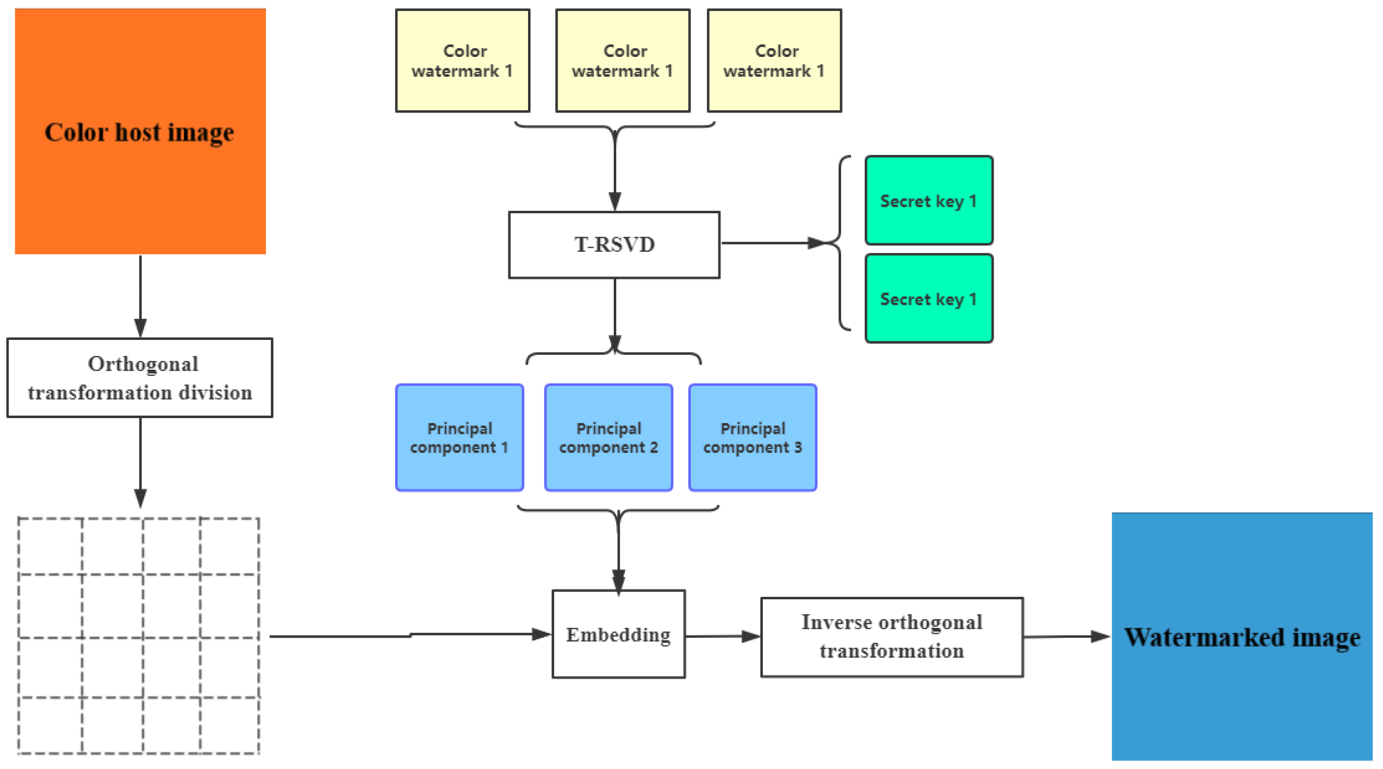
- A1.
- T-RSVD-based decomposes three color watermark images , and ,where and are the secret keys and are saved to extract the implanted watermarks.
- A2.
- Calculate the main components of each color watermark image,
- A3.
- Orthogonal transformation divides the color host image into several non-overlapping color image blocks of size , and is the orthogonal transformed image on block position , , where .
- A4.
- Implant the main components , and into the transformed color host image blocks , and :where is a scale factor used to control watermarking strength [23]. When the value of is actually confirmed, the larger is, the stronger the robustness of the watermark is, and the weaker the invisibility of the watermark is. The balance between robustness and invisibility needs to be considered. Save , and to guarantee the extraction.
- A5.
- Implement inverse orthogonal transformation for all image blocks , and gain the watermarked color image .
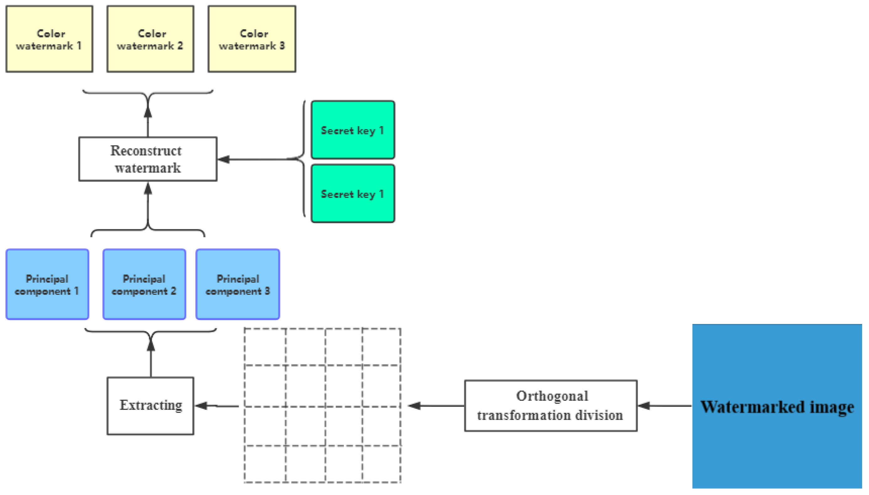
- B1.
- Split the watermarked color image into several non-overlapping color image blocks with size , .
- B2.
- Extract the main components of each color watermark image as follows:
- B3.
- Calculate the extracted watermarks , , and :
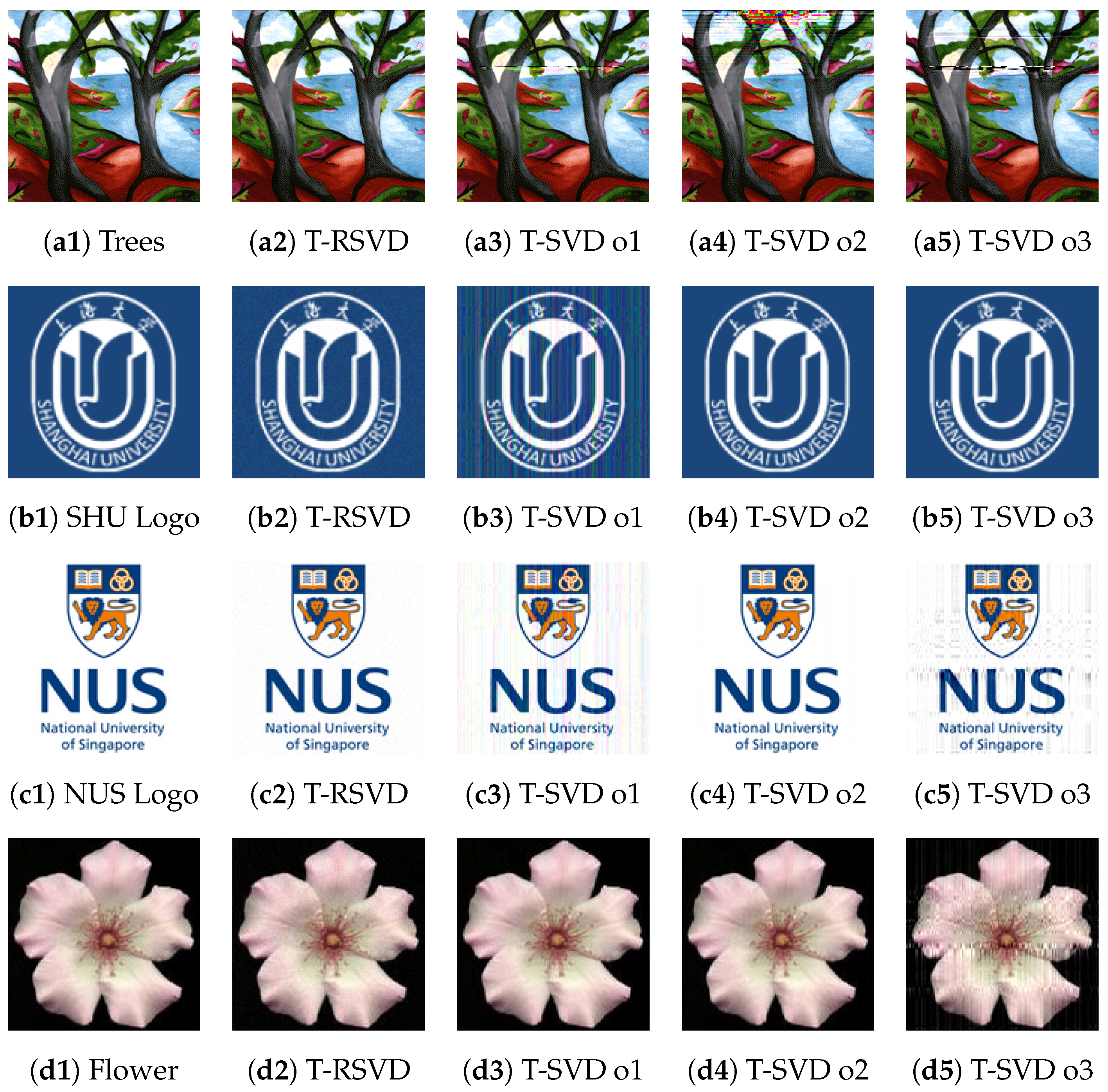
- Order 1: SHU Logo →NUS Logo →Flower;
- Order 2: NUS Logo →Flower →SHU Logo;
- Order 3: Flower →NUS Logo →SHU Logo.
5. Conclusions and Prospects
Author Contributions
Funding
Data Availability Statement
Acknowledgments
Conflicts of Interest
References
- Comon, P.; Luciani, X.; De Almeida, A.L. Tensor decompositions, alternating least squares and other tales. J. Chemom. 2009, 23, 393–405. [Google Scholar] [CrossRef]
- Doostan, A.; Iaccarino, G.; Etemadi, N. A least-squares approximation of high-dimensional uncertain systems. In Annual Research Briefs; Center for Turbulence Research, Stanford University: Stanford, CA, USA, 2007; pp. 121–132. [Google Scholar]
- He, Z.H.; Ng, M.K.; Zeng, C. Generalized singular value decompositions for tensors and their applications. Numer. Math. Theory Methods Appl. 2021, 14, 692–713. [Google Scholar] [CrossRef]
- Jin, H.; Bai, M.; Benítez, J.; Liu, X. The generalized inverses of tensors and an application to linear models. Comput. Math. Appl. 2017, 74, 385–397. [Google Scholar] [CrossRef]
- Omberg, L.; Golub, G.H.; Alter, O. A tensor higher-order singular value decomposition for integrative analysis of DNA microarray data from different studies. Proc. Natl. Acad. Sci. USA 2007, 104, 18371–18376. [Google Scholar] [CrossRef]
- Savas, B.; Eldén, L. Handwritten digit classification using higher order singular value decomposition. Pattern Recognit. 2007, 40, 993–1003. [Google Scholar] [CrossRef]
- Shashua, A.; Hazan, T. Non-negative tensor factorization with applications to statistics and computer vision. In Proceedings of the 22nd International Conference on Machine Learning, Bonn Germany, 7–11 August 2005; pp. 792–799. [Google Scholar]
- Song, G.; Ng, M.K.; Zhang, X. Robust tensor completion using transformed tensor singular value decomposition. Numer. Linear Algebra Appl. 2020, 27, e2299. [Google Scholar] [CrossRef]
- De Lathauwer, L.; De Moor, B.; Vandewalle, J. A multilinear singular value decomposition. SIAM J. Matrix Anal. Appl. 2000, 21, 1253–1278. [Google Scholar] [CrossRef]
- Kolda, T.G.; Bader, B.W. Tensor decompositions and applications. SIAM Rev. 2009, 51, 455–500. [Google Scholar] [CrossRef]
- Miao, Y.; Qi, L.; Wei, Y. Generalized tensor function via the tensor singular value decomposition based on the T-product. Linear Algebra Its Appl. 2020, 590, 258–303. [Google Scholar] [CrossRef]
- Zhang, J.; Saibaba, A.K.; Kilmer, M.E.; Aeron, S. A randomized tensor singular value decomposition based on the t-product. Numer. Linear Algebra Appl. 2018, 25, e2179. [Google Scholar] [CrossRef]
- Zeng, C.; Ng, M.K. Decompositions of third-order tensors: HOSVD, T-SVD, and Beyond. Numer. Linear Algebra Appl. 2020, 27, e2290. [Google Scholar] [CrossRef]
- Kilmer, M.E.; Braman, K.; Hao, N.; Hoover, R.C. Third-order tensors as operators on matrices: A theoretical and computational framework with applications in imaging. SIAM J. Matrix Anal. Appl. 2013, 34, 148–172. [Google Scholar] [CrossRef]
- Martin, C.D.; Shafer, R.; LaRue, B. An order-p tensor factorization with applications in imaging. SIAM J. Sci. Comput. 2013, 35, A474–A490. [Google Scholar] [CrossRef]
- Hao, N.; Kilmer, M.E.; Braman, K.; Hoover, R.C. Facial recognition using tensor-tensor decompositions. SIAM J. Imaging Sci. 2013, 6, 437–463. [Google Scholar] [CrossRef]
- Kilmer, M.E.; Martin, C.D. Factorization strategies for third-order tensors. Linear Algebra Its Appl. 2011, 435, 641–658. [Google Scholar] [CrossRef]
- Cox, I.; Miller, M.; Bloom, J.; Fridrich, J.; Kalker, T. Digital Watermarking and Steganography; Morgan Kaufmann: Burlington, MA, USA, 2007. [Google Scholar]
- Mintzer, F.; Braudaway, G.W. If one watermark is good, are more better? In Proceedings of the 1999 IEEE International Conference on Acoustics, Speech, and Signal Processing. Proceedings. ICASSP99 (Cat. No.99CH36258), Phoenix, AZ, USA, 15–19 March 1999; Volume 4, pp. 2067–2069. [Google Scholar]
- Miao, Y.; Qi, L.; Wei, Y. T-Jordan canonical form and T-Drazin inverse based on the T-product. Commun. Appl. Math. Comput. 2021, 3, 201–220. [Google Scholar] [CrossRef]
- De Moor, B.L.; Golub, G.H. The restricted singular value decomposition: Properties and applications. SIAM J. Matrix Anal. Appl. 1991, 12, 401–425. [Google Scholar] [CrossRef]
- Chu, D.; De Lathauwer, L.; De Moor, B. On the computation of the restricted singular value decomposition via the cosine-sine decomposition. SIAM J. Matrix Anal. Appl. 2000, 22, 580–601. [Google Scholar] [CrossRef]
- Harjito, B.; Prasetyo, H. False-positive-free GSVD-based image watermarking for copyright protection. In Proceedings of the 2016 International Symposium on Electronics and Smart Devices (ISESD), Bandung, Indonesia, 29–30 November 2016; pp. 143–147. [Google Scholar]
- Lai, C.C.; Tsai, C.C. Digital image watermarking using discrete wavelet transform and singular value decomposition. IEEE Trans. Instrum. Meas. 2010, 59, 3060–3063. [Google Scholar] [CrossRef]
- Chen, Y.; Wang, Q.W.; Xie, L.M. Dual quaternion matrix equation AXB=C with applications. Symmetry 2024, 16, 287. [Google Scholar] [CrossRef]
- Zhang, Y.; Wang, Q.W.; Xie, L.M. The Hermitian solution to a new system of commutative quaternion matrix equations. Symmetry 2024, 16, 361. [Google Scholar] [CrossRef]


| Method | PSNR (dB) | Time (s) | |||||
|---|---|---|---|---|---|---|---|
| Trees | SHU Logo | NUS Logo | Flower | Embedding | Extracting | ||
| Order 1 | T-RSVD | 36.5237 | 34.0030 | 33.9725 | 33.9886 | 1.1875 | 0.0937 |
| T-SVD | 25.2867 | 24.1887 | 24.7375 | 73.9727 | 1.9218 | 0.0937 | |
| Order 2 | T-RSVD | 36.5237 | 34.0198 | 33.9450 | 33.9722 | 1.1250 | 0.0937 |
| T-SVD | 12.4073 | 73.9771 | 52.6427 | 52.1781 | 2.1562 | 0.1250 | |
| Order 3 | T-RSVD | 36.5237 | 33.9610 | 33.9461 | 33.9553 | 1.2187 | 0.0781 |
| T-SVD | 17.6431 | 73.9833 | 25.3310 | 24.7176 | 2.1093 | 0.0937 | |
Disclaimer/Publisher’s Note: The statements, opinions and data contained in all publications are solely those of the individual author(s) and contributor(s) and not of MDPI and/or the editor(s). MDPI and/or the editor(s) disclaim responsibility for any injury to people or property resulting from any ideas, methods, instructions or products referred to in the content. |
© 2024 by the authors. Licensee MDPI, Basel, Switzerland. This article is an open access article distributed under the terms and conditions of the Creative Commons Attribution (CC BY) license (https://creativecommons.org/licenses/by/4.0/).
Share and Cite
Zhang, C.-Q.; Wang, Q.-W.; Wang, X.-X.; He, Z.-H. Restricted Singular Value Decomposition for a Tensor Triplet under T-Product and Its Applications. Mathematics 2024, 12, 982. https://doi.org/10.3390/math12070982
Zhang C-Q, Wang Q-W, Wang X-X, He Z-H. Restricted Singular Value Decomposition for a Tensor Triplet under T-Product and Its Applications. Mathematics. 2024; 12(7):982. https://doi.org/10.3390/math12070982
Chicago/Turabian StyleZhang, Chong-Quan, Qing-Wen Wang, Xiang-Xiang Wang, and Zhuo-Heng He. 2024. "Restricted Singular Value Decomposition for a Tensor Triplet under T-Product and Its Applications" Mathematics 12, no. 7: 982. https://doi.org/10.3390/math12070982
APA StyleZhang, C.-Q., Wang, Q.-W., Wang, X.-X., & He, Z.-H. (2024). Restricted Singular Value Decomposition for a Tensor Triplet under T-Product and Its Applications. Mathematics, 12(7), 982. https://doi.org/10.3390/math12070982