Exploring the Entropy-Based Classification of Time Series Using Visibility Graphs from Chaotic Maps

Abstract

The classification of time series using machine learning (ML) analysis and entropy-based features is an urgent task for the study of nonlinear signals in the fields of finance, biology and medicine, including EEG analysis and Brain–Computer Interfacing. As several entropy measures exist, the problem is assessing the effectiveness of entropies used as features for the ML classification of nonlinear dynamics of time series. We propose a method, called global efficiency (GEFMCC), for assessing the effectiveness of entropy features using several chaotic mappings. GEFMCC is a fitness function for optimizing the type and parameters of entropies for time series classification problems. We analyze fuzzy entropy (FuzzyEn) and neural network entropy (NNetEn) for four discrete mappings, the logistic map, the sine map, the Planck map, and the two-memristor-based map, with a base length time series of 300 elements. FuzzyEn has greater GEFMCC in the classification task compared to NNetEn. However, NNetEn classification efficiency is higher than FuzzyEn for some local areas of the time series dynamics. The results of using horizontal visibility graphs (HVG) instead of the raw time series demonstrate the GEFMCC decrease after HVG time series transformation. However, the GEFMCC increases after applying the HVG for some local areas of time series dynamics. The scientific community can use the results to explore the efficiency of the entropy-based classification of time series in “The Entropy Universe”. An implementation of the algorithms in Python is presented.

1. Introduction

The classification of time series based on entropy analysis and machine learning (ML) is a trending task in the study of nonlinear signals in the fields of finance, biology, and medicine, for example, in EEG classification in diagnosing Alzheimer’s disease [1,2] and Parkinson’s disease [3,4,5,6]. The creation of Brain–Computer Interfacing (BCI) [7] enables the classification of the movements of body parts according to EEG signals. Such developments may benefit people who lose their mobility due to the communication breakup between the brain and limb muscles. BCI helps people to move their limbs with the help of an external robotic device called the exoskeleton. Classifying temperature time series can help doctors to classify patients as patients with fever and healthy individuals [8]. Using entropy to analyze electromyography (EMG) signals is a necessary step in diagnosing neuromuscular diseases [9]. An alternative non-invasive and inexpensive diagnosis of the knee joint uses vibration-artographic signals. Sound signals emitted by the patellofemoral joint contain information that can characterize the pathological aspect of the knee joint lesion and are classified by entropy characteristics [10]. Time series forecasting using entropy features is widely used in the financial industry in applications such as the forecasting of stock market prices and commodity prices [11].

There are many types of entropies, which in turn have several customizable parameters; for example, sample entropy (SampEn) [12], cosine similarity entropy (CoSiEn) [13], singular value decomposition entropy (SVDEn) [14], fuzzy entropy (FuzzyEn) [3,15,16,17,18], permutation entropy (PermEn) [19], etc. A promising research direction is the development of new types of entropies or modifications of known entropy types [20,21]. Recently, Velichko et al. proposed the use of a LogNNet neural network [22] for neural network entropy (NNetEn) calculation [1]. LogNNet neural network is a feedforward neural network that uses filters based on the logistic function and a reservoir inspired by recurrent neural networks, thus enabling the transformation of a signal into a high-dimensional space. Its efficiency was validated on the MNIST-10 dataset [23]. This showed that the classification performance is proportional to the entropy of the time series and has a stronger correlation than the Lyapunov exponent of the time series used to feed the reservoir.

Before calculating an entropy function, several parameters should be initialized, for example, embedding dimension m, tolerance threshold r, and time series length N. Although these parameters are critical for calculations, there are no guidelines for optimizing parameter values, as there is no generally accepted fitness function. Several authors have conducted research on optimal parameters and types of entropy [24,25,26,27,28], and this research does not claim to be general. The conclusions are of a local nature, characterized by the time series databases and the entropies used. A wide variety of entropies exists: the EntropyHub Guide lists 18 types of entropies [29,30], and the review by Ribeiro et al. [31] compares 40 types of entropies for various areas of application and coins the term “The Entropy Universe”. In this context, it is important to assess the effectiveness of the different entropies when used as features in ML classification. In the current study, we assume that global entropy efficiency can be calculated on model time series generated by chaotic mappings. The method includes a wide range of time series with different dynamics, and the calculated entropy efficiency value (GEFMCC) can be considered a global entropy characteristic for time series classification problems. The GEFMCC’s value is as a fitness function for optimization problems when searching for the best entropies for time series classification problems. We present a Python implementation for calculating the generalized efficiency of FuzzyEn and NNetEn entropy for user-specified parameters. Using this method, it is possible to not only rank the existing entropies, but also evaluate the effectiveness of new types of entropies for time series classification problems.

The effectiveness of using FuzzyEn and NNetEn was shown on EEG signals in diagnosing Alzheimer’s disease [1]. The effectiveness of fuzzy entropy in diagnosing Parkinson’s disease was also demonstrated in the paper by Belyaev et al. [3]. It was experimentally shown that FuzzyEn has an advantage over other entropies when classifying EEG signals with several elements in a time series of ~100–1000. As a result, the authors of this work had the idea of studying whether or not the efficiency of FuzzyEn is universal and applicable to a series of different dynamics. In this paper, the authors analyzed two entropies, FuzzyEn and NNetEn, with the most effective settings taken from the works [1,3], and conducted a test on artificially created databases based on chaotic mappings. In addition, we explored the option of preprocessing time series using HVG transformation.

The natural visibility graph (NVG) was introduced in [32] as a simple and computationally efficient method to represent a time series as a graph. Visibility graphs preserve the periodic and chaotic properties of the discrete map [32]; see [33,34,35]. For example, periodic series result in regular graphs, random series in random graphs, and fractal series in scale-free graphs. Horizontal visibility graphs (HVG) were introduced in [32] to simplify the previously described NVG. Visibility graphs (VG) reduce the complexity of calculations, which depends on time series, while preserving the accuracy of the results; see [36,37,38].

In [39], the authors described the advantages of using the amplitude difference distribution instead of the degree distribution to collect information from the network formed by the horizontal visibility graph. Li and Shang introduced a combination of the amplitude difference distribution with discrete generalized past entropy to present a new method called discrete generalized past entropy based on the amplitude difference distribution of the horizontal visibility graph (AHVG-DGPE). The authors note its efficiency in systems evaluation and its higher accuracy and sensitivity rate than the traditional method in characterizing dynamic systems; see [40,41,42].

In this paper, we propose a method for assessing the effectiveness of entropies using chaotic mapping. We use it for analyzing the FuzzyEn and NNetEn entropies on four discrete mappings: the logistic map, the sine map, the Planck map, and the two-memristor-based map. We utilize the corresponding HVG degrees’ representation of these time series, which implies that the resulting time series does not consist of real numbers but only of integer numbers. The results of using horizontal visibility graphs (HVG) to classify time series are also shown.

The major contributions of the paper are as follows:

• A concept for comparing the efficiency of classifying chaotic time series using entropy-based features is presented. The developed methodology can be used in classification problems for financial, biological, and medical signals.
• A new characteristic for assessing the global efficiency of entropy (GEFMCC) is presented. GEFMCC is calculated based on synthetic databases generated by four chaotic mappings.
• The Python package for GEFMCC calculation is developed.
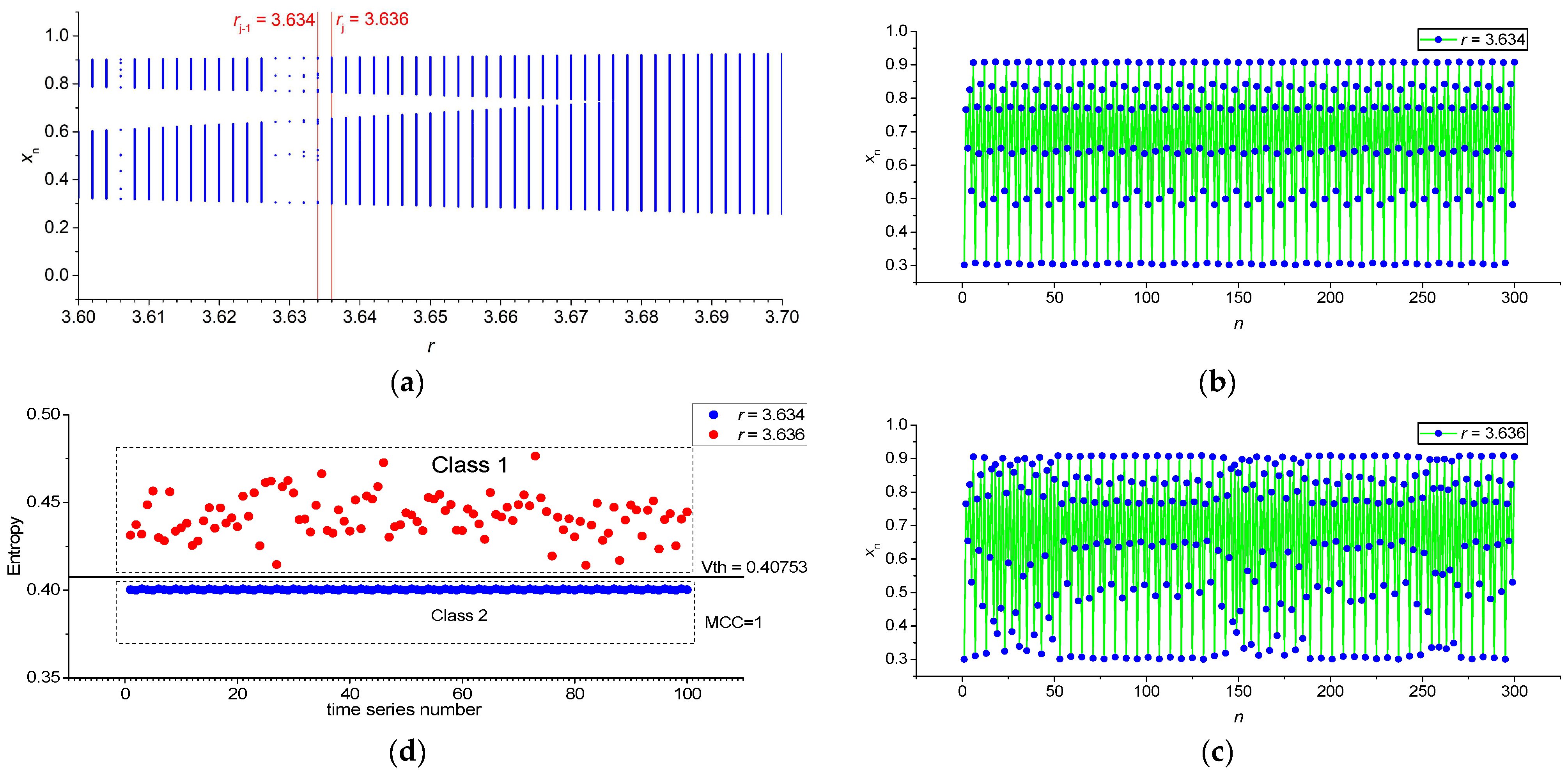
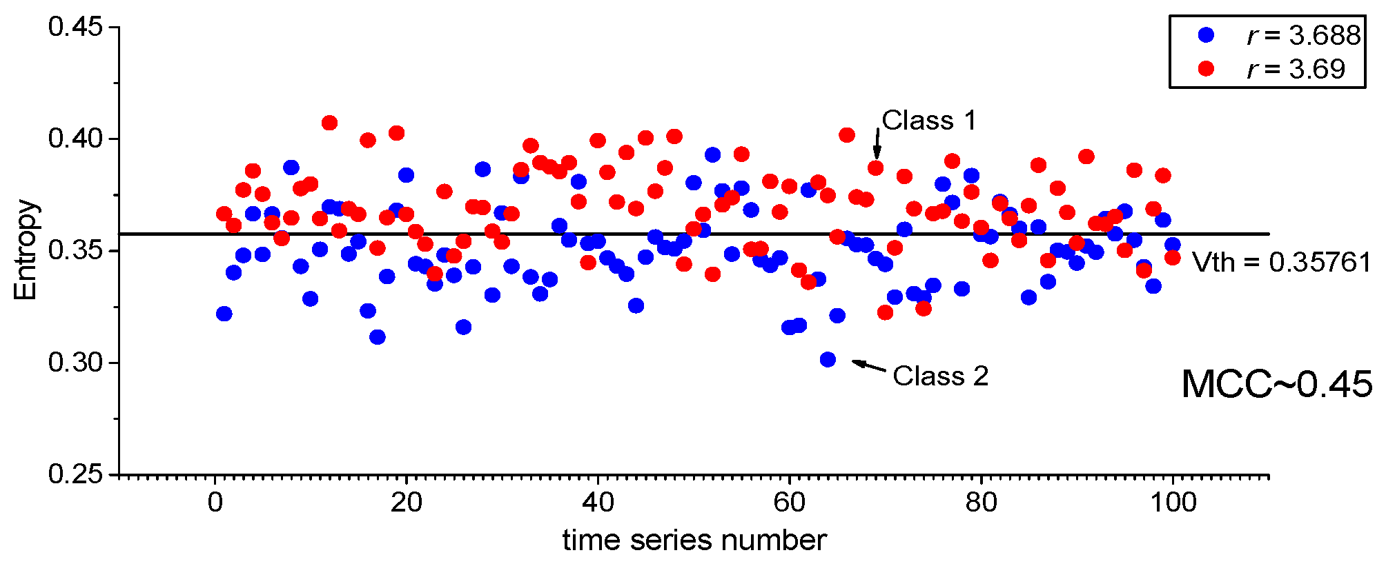
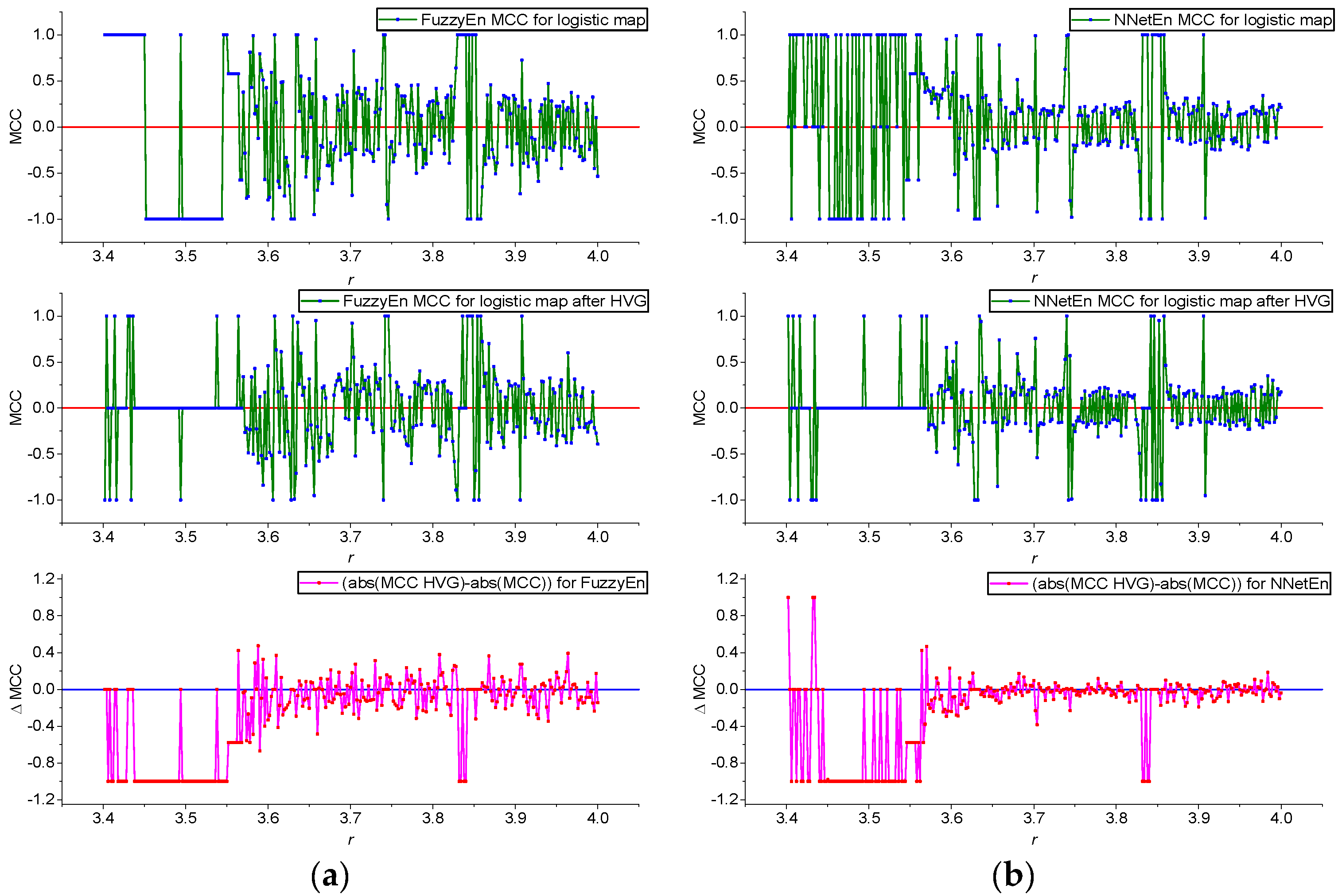
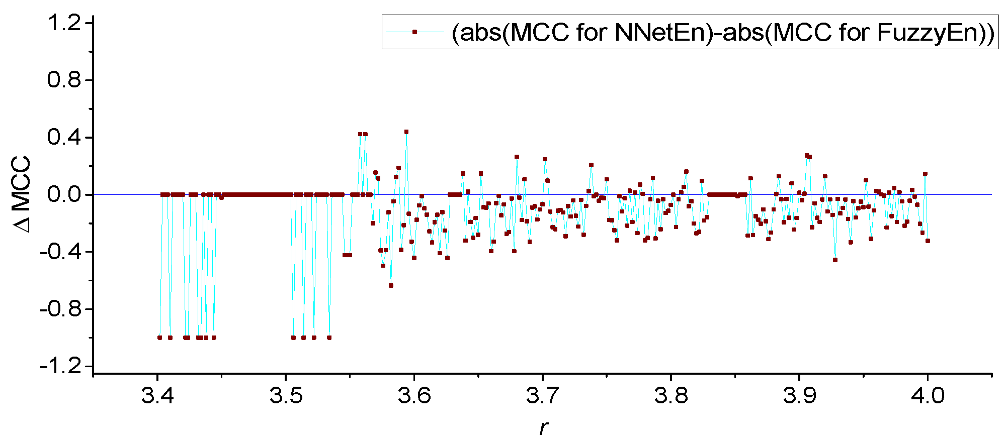
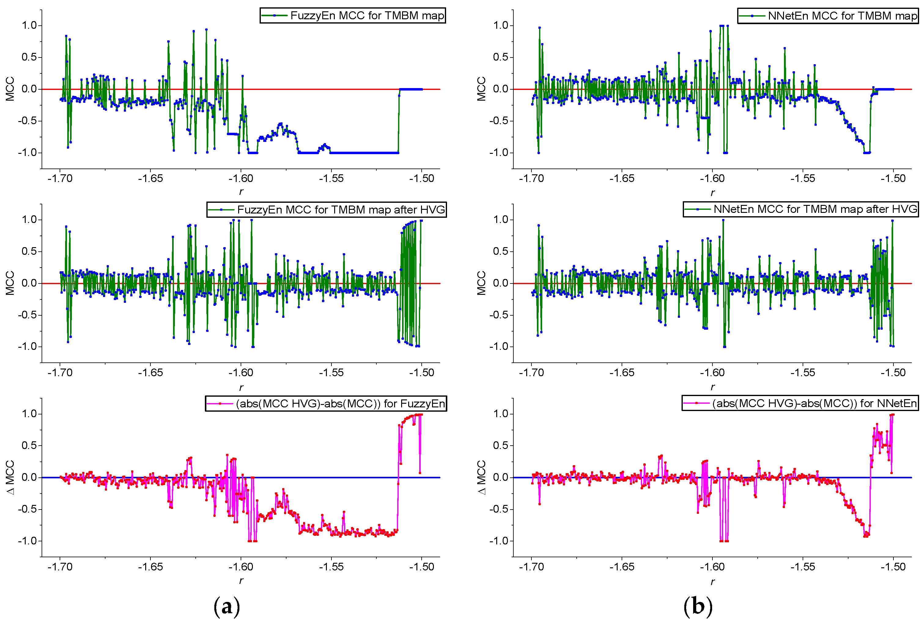
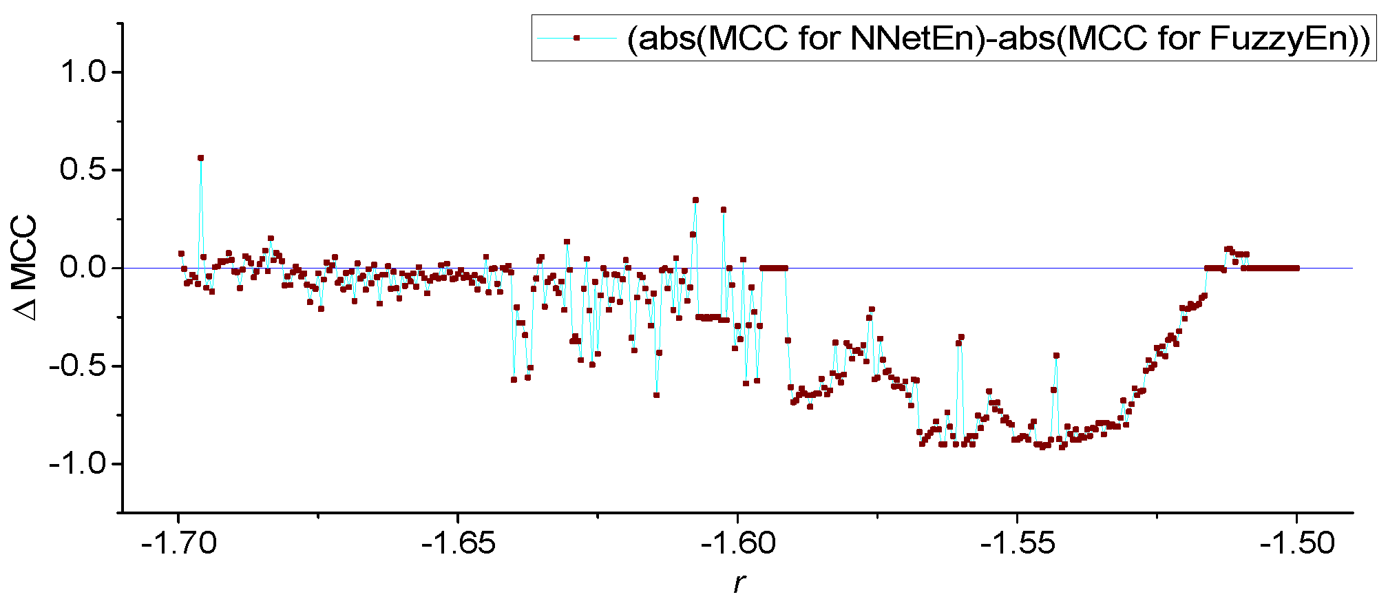
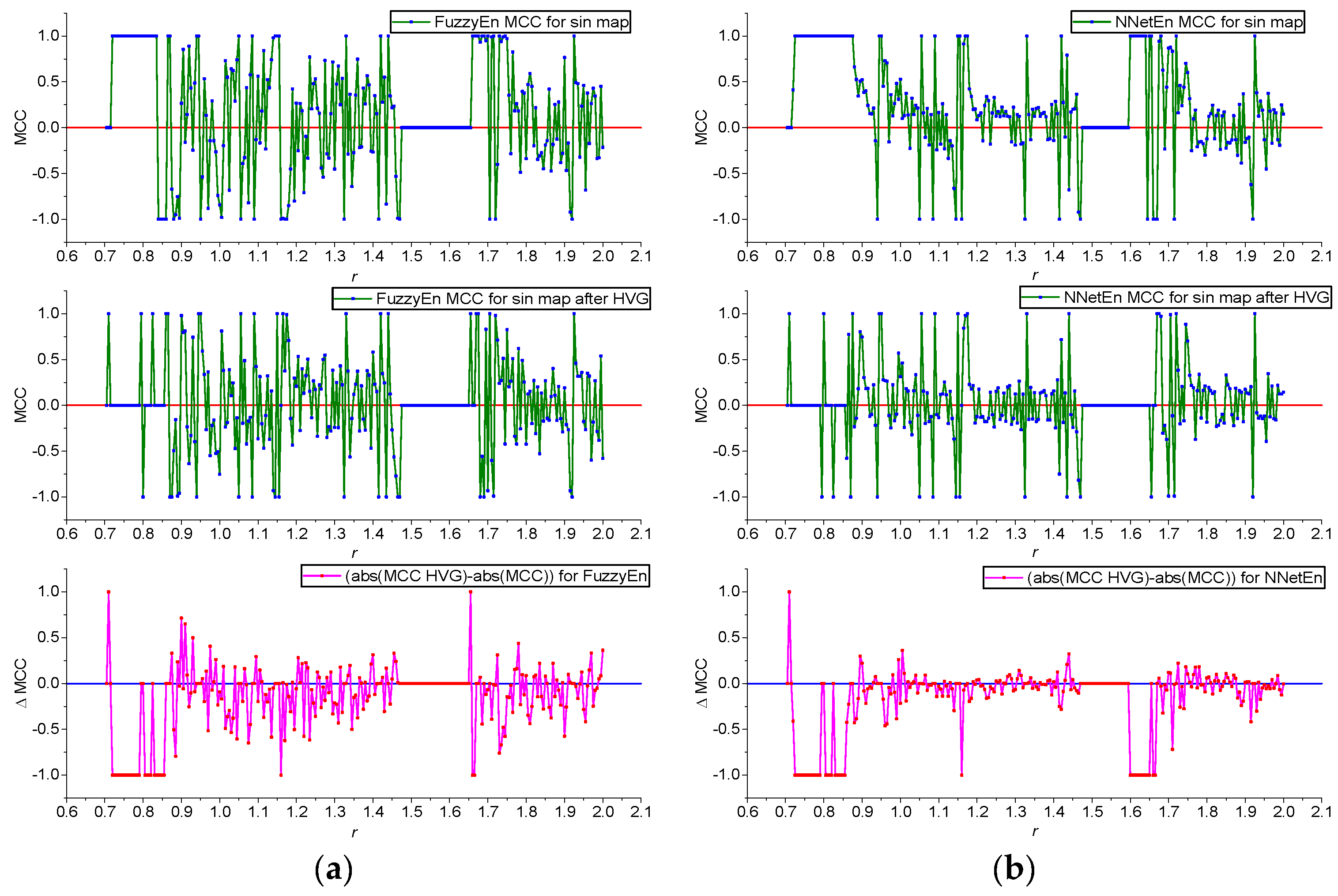
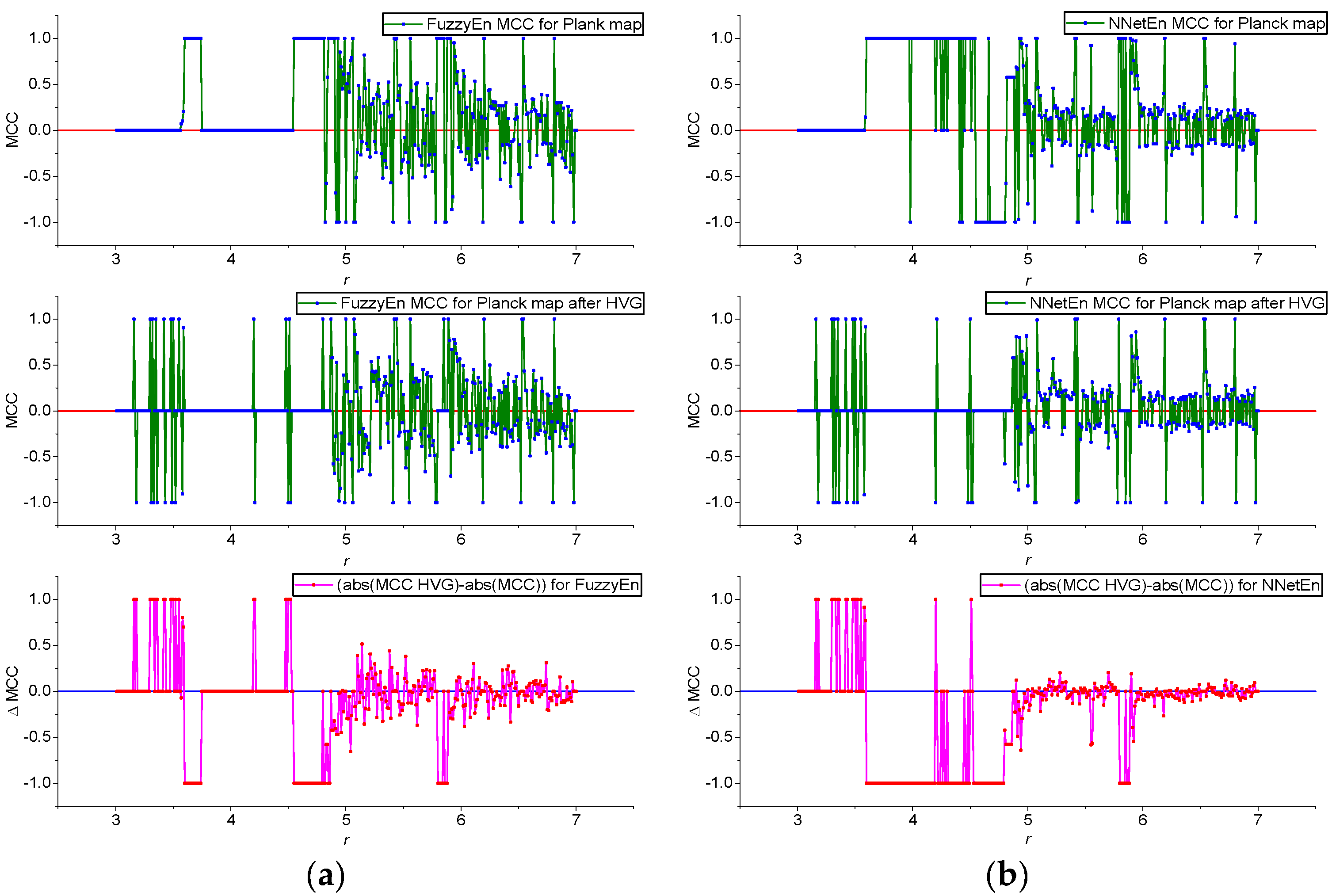
• A comparison of the effectiveness of FuzzyEn (m = 1, r = 0.2∙d, r₂ = 3, τ = 1) and NNetEn (D1, 1, M3, Ep5, Acc) was investigated. FuzzyEn is shown to have improved GEFMCC in the classification task compared to NNetEn. At the same time, there are local areas of the time series dynamics in which the classification efficiency NNetEn is higher than FuzzyEn. The Matthews correlation coefficient was used to evaluate binary classification.
• The results of using HVG are shown. GEFMCC decreases after HVG time series transformation, but there are local areas of time series dynamics in which the classification efficiency increases after HVG.

This paper is organized as follows: Section 2 introduces the methods we have used. In Section 3, we explain the results we obtained. Section 4 discusses the results and states the conclusions, and outlines some ideas for future works.

2. Materials and Methods

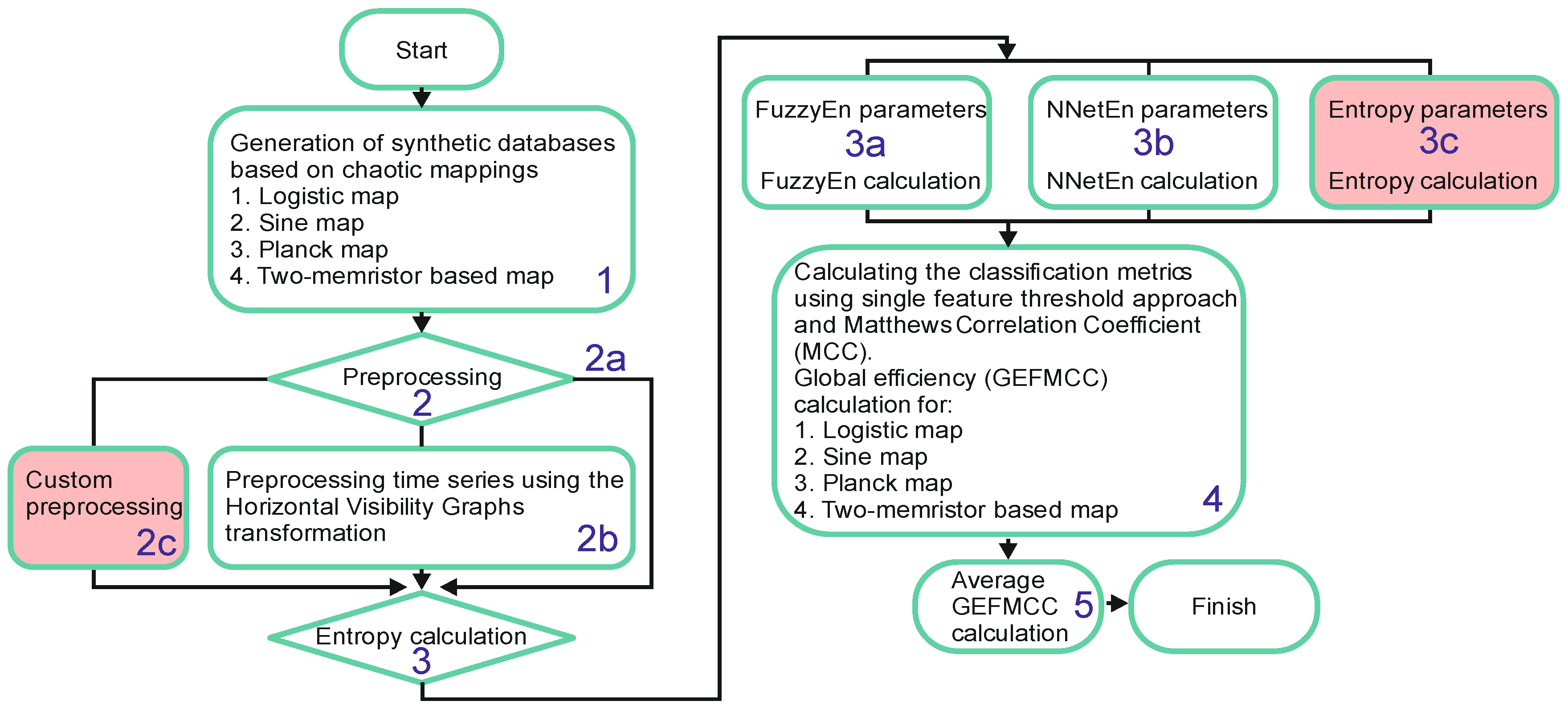
2.1. The Workflow Diagram of the Proposed Method

Figure 1 presents the overall workflow diagram of the proposed method for assessing the global entropy efficiency.

Stage 1: Synthetic databases are generated based on four types of discrete chaotic maps: logistic map, sine map, Planck map, and two-memristor-based map.

Stage 2: The method for pre-processing synthetic time series is selected. In this study, we used ‘no pre-processing’ in Stage 2a, and pre-processing based on the horizontal visibility graphs transformation method in Stage 2b. In further studies, optional custom pre-processing can be performed (Stage 2c), for example, by applying a combination of adding noise and HVG transformation.

Stage 3: The type and entropy parameters for calculating GEFMCC values for each chaotic mapping are selected. In this study, we used FuzzyEn (Stage 3a) with parameters (m = 1, r = 0.2∙d, r₂ = 3, τ = 1) and NNetEn (Stage 3b) with parameters (D1, 1, M3, Ep5, ACC). In further research (Stage 3c), any other type of entropy can be used, such as SampEn, CoSiEn, SVDEn, PermEn, etc. After selecting the type and parameters of entropy, the entropies of the time series in each synthetic dataset are calculated.

Stage 4: The databases are classified using the single feature threshold approach and the Matthews correlation coefficient as a metric. The GEFMCC value for each chaotic mapping is calculated.

Stage 5: For all chaotic mappings, the average GEFMCC value is calculated and represents the efficiency of entropy.

In the following sections, we explain the individual steps of the method in more detail.

2.2. Generation of Synthetic Time Series (Stage 1)

To generate synthetic time series, we used several types of discrete chaotic map. The control parameter r_j (j = 1… Nr) varied discretely with step dr.

• Logistic map [43,44]:

$$x_{n+1}=r_j\cdot x_n\cdot (1-x_n), 3.4 \le r_j\le 4, x_{-999}=0.1, dr=0.002, r_1=3.4, Nr=301$$

(1)

2.

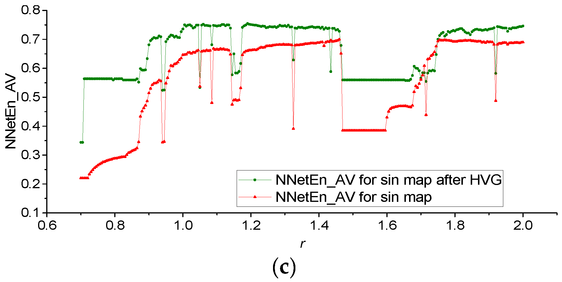
Sine map [45]:

$$x_{n+1}=r_j\cdot \sin (\pi \cdot x_n), 0.7 \le r_j\le 2, x_{-999}=0.1, dr=0.005, r_1=0.7, Nr=261$$

(2)

3.

Planck map [45]:

$$x_{n+1}=\frac{r_j\cdot x_n^3}{1+e^{x_n}}, 3 \le r_j\le 7, x_{-999}=4, dr=0.01, r_1=3, Nr=401$$

(3)

4.

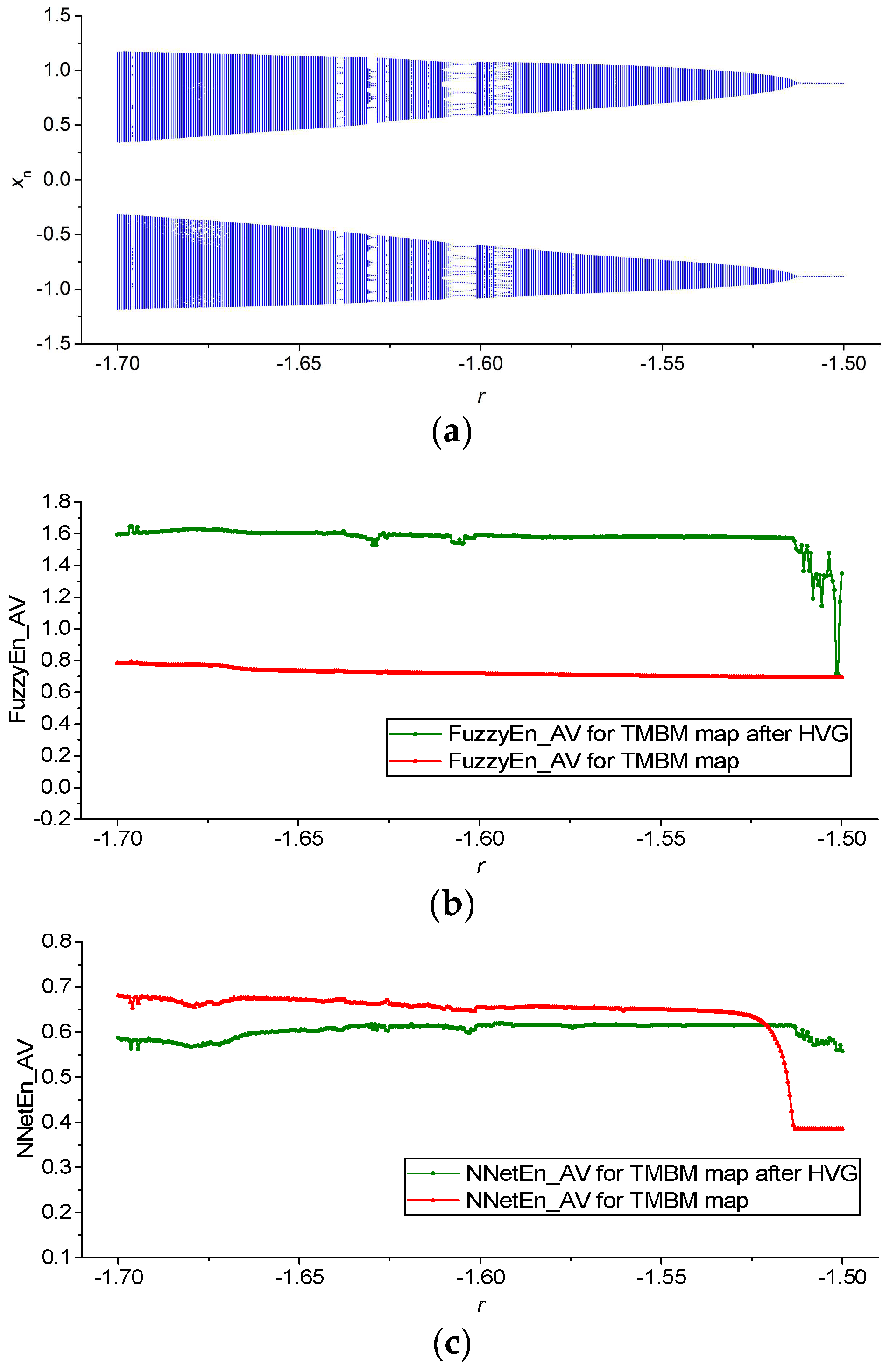
Two-memristor-based map (TMBM) [46]:

$$\begin{array}{l}\{\begin{array}{l}{x}_{n+1}=r_j\cdot a_2\cdot (b\cdot \left|y_n\right|-1)\cdot (z_n^2-1)\cdot x_n+c\\ y_{n+1}=y_n+x_n\\ z_{n+1}=z_n+r_j\cdot (b\cdot \left|y_n\right|-1)\cdot x_n\end{array}, -1.7 \le r_j\le -1.5\\ x_{-999}=0.01, y_{-999}=0.01, z_{-999}=0.01, dr=0.0005, r_1=-1.7, Nr=401\end{array}$$

(4)

The first 1000 elements (x₋₉₉₉… x₀) are ignored due to the transient period. If n > 0, then the time series are calculated for x_n. To generate a class corresponding to one value of r_j, 100 time series were generated with a length of N = 300 elements. Elements in each series were calculated sequentially: (x₁, …, x₃₀₀), (x₃₀₁, …, x₆₀₀), etc. A set of NE = 100 time series was generated at a given r_j. The value r_j ran through the entire range with a certain step dr; see Equations (1)–(4).

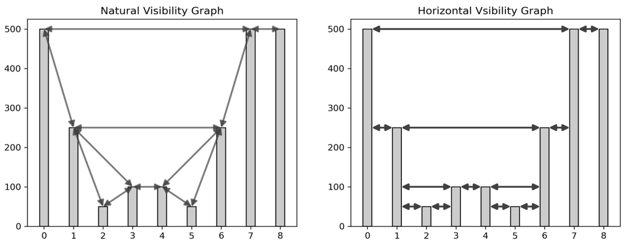
2.3. Natural and Horizontal Visibility Graphs (Stage 2b)

In the present study, we explored the option of preprocessing time series using the HVG transformation. Let us briefly describe its essence.

Given a time series {(n, x_n)}_n∈ℕ indexed on the set of natural numbers ℕ, such that at time n, the time series takes the value x_n, an association is found between each node and each pair (n, x_n) in order to obtain the graph associated with the time series. A natural visibility graph (NVG) is constructed as follows: given two nodes (n, x_n) and (m, x_m), these two nodes have visibility, and thus they are connected in the graph by an edge if any other pair (c, x_c) with n < c < m satisfies

$$x_c<x_m+(x_n-x_m)\frac{m-c}{m-n}$$

(5)

Horizontal visibility graphs (HVG) were introduced in [32] to simplify the requirements described for NVG.

When computing the HVG, each time series value is related to a node in the resulting graph, as in the case of NVG. Two nodes in this graph, (n, x_n) and (m, x_m), are connected if a horizontal line can be drawn connecting their corresponding visibility index without intersecting any intermediate value, that is, if x_n, x_m > x_c for all n < c < m; see the examples in Figure 2.

Python 3.11 library ts2vg (version 1.2.3) was used to calculate HVG (‘time series to visibility graphs’) [47], which implements algorithms for plotting graphs based on time series data. The package utilizes a highly effective C backend for its operations (using Cython) and seamlessly integrates with the Python environment. As a result, ts2vg can effortlessly process input data from various sources using established Python tools. Additionally, it enables the examination and interpretation of the generated visibility graphs using a wide range of techniques including graph analysis, data science, visualization packages, and tools compatible with Python. The HorizontalVG method was used to construct the HVG.

2.4. FuzzyEn Calculation (Stage 3a)

FuzzyEn entropy was introduced as an advancement of the concepts of approximate entropy (ApEn) and sample entropy (SampEn) to overcome some of their shortcomings, such as dependence on data length and intrinsic biases. FuzzyEn is proposed as a measure more robust to noise and is used for analyzing the complexity of time series data. Unlike ApEn and SampEn, which apply the Heaviside function to calculate differences between vectors [48], FuzzyEn uses exponential functions with fuzzy boundaries.

Fuzzy entropy can be calculated as follows. For a given time series $X=\left[x_1,x_2,\dots ,x_N\right]$ with given embedding dimension $\left(m\right)$, $X_m$ vectors will form as:

$$X_m\left(i\right)=\left[x_i,x_{i+1},\dots ,x_{i+m-1}\right]-{x0}_i$$

(6)

These vectors represent $m$ consecutive $x$ values, starting with the $i\mathrm{t}\mathrm{h}$ point, with the baseline ${x0}_i=\frac{1}{m}{\sum }_{j=0}^{m-1}{x}_{i+j}$ removed. Then, the distance between vectors $X_m\left(i\right)$ and $X_m\left(j\right)$, $d_{ij,m}$ can be defined as the maximum absolute difference between their scalar components. Given $n$ and $r$, the degree of similarity $D_{ij,m}$ of the vectors $X_m\left(i\right)$ and $X_m\left(j\right)$ is calculated using fuzzy function.

$$D_{ij,m}=\mu \left(d_{ij,m},r\right)=exp\left(\frac{-{\left(d_{ij,m}\right)}^n}{r}\right)$$

(7)

The function ${\varphi }_m$ is defined as

$${\varphi }_m\left(n,r\right)=\frac{1}{N-m}{\sum }_{i=1}^{N-m}\left(\frac{1}{N-m-1}{\sum }_{j=1,j\ne i}^{N-m}{D}_{ij,m}\right)$$

(8)

Repeating the same procedure from Equations (9) and (10) for the dimension to $m+1$, vectors $X_{m+1}\left(i\right)$ are formed and the function ${\varphi }_{m+1}$ is obtained. Therefore, FuzzyEn can be estimated as:

$$FuzzyEn\left(m,n,r,N\right)=ln{\varphi }_m\left(n,r\right)-ln{\varphi }_{m+1}\left(n,r\right)$$

(9)

FuzzyEn represents a measure of irregularity in a time series, taking into account the spatial and temporal characteristics of the data.

The EntropyHub library [49] (version 0.2) allows for the reliable and standardized calculation of FuzzyEn, essential for comparing results across different studies. EntropyHub integrates the many established entropy methods into one package, available for Python, MatLab and Julia users. In the computation of FuzzyEn, the embedding dimension m = 1 and tolerance r = 0.2 × std were used in the analysis, where std is a standard deviation of $x_n$, argument exponent (pre-division) r₂ = 3, and time delay $\tau =1$.

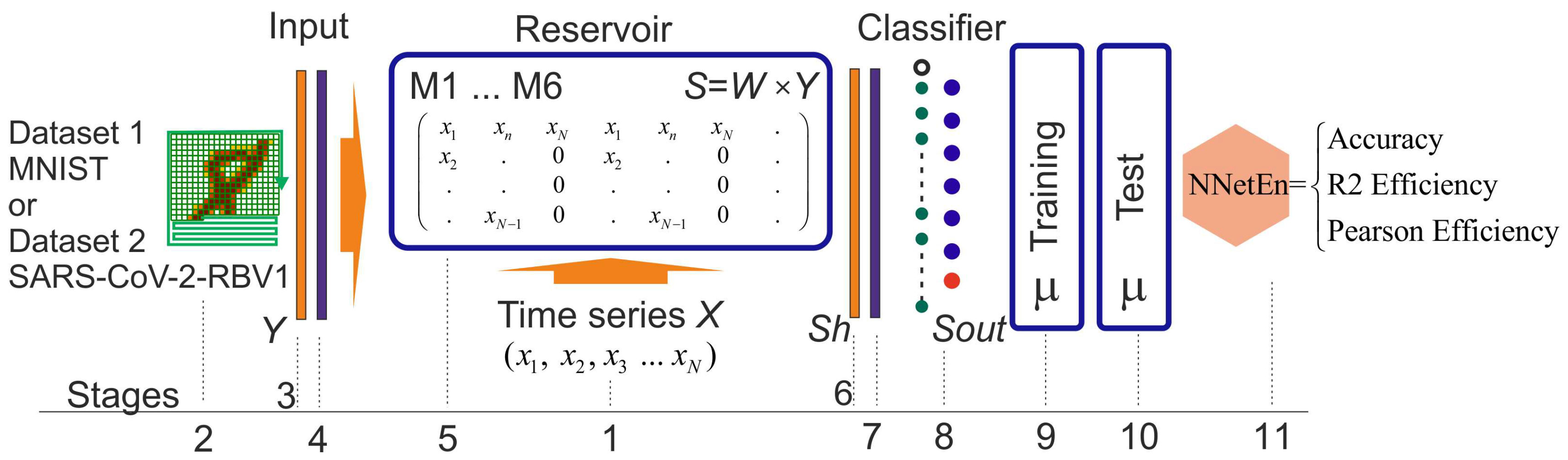
2.5. NNetEn Calculation (Stage 3b)

The NNetEn calculation method is based on the reservoir neural network LogNNet [22,50], where the reservoir is filled with the time series under study, and the entropy value is proportional to the classification metric of the reference database. The principle of calculating entropy is fundamentally different from all known modifications of entropy based on the probability distribution. Figure 3 shows the process for calculating NNetEn [1]. The method involves several key steps, which are detailed below.

Step 1: The initial step encompasses inputting the time series $X=\left[x_1,x_2,\dots ,x_N\right]$ of length N into the reservoir.

Six main methods for filling the reservoir were researched in detail. The M1 to M6 methods involve various techniques for filling the reservoir. They are M1—row-wise filling with duplication; M2—row-wise filling with an additional zero element; M3—row-wise filling with time series stretching; M4—column-wise filling with duplication; M5—column-wise filling with an additional zero element; and M6—column-wise filling with time series stretching.

Step 2: Selection of embedded dataset 1 (MNIST-10 [51]) or dataset 2 (SARS-CoV-2-RBV1 [1]), upon which the classification metrics will be computed. These databases are included in the Python library for NNetEn calculations and are selected with the parameter database = ‘D1’ or database = ‘D2’.

Step 3: Formation of the Y vector from the dataset, including a zero offset Y [0] = 1.

Step 4: Normalization of the Y vector.

Step 5: Multiplication of the Y vector with the reservoir matrix and the input vector Sh = W × Y to convert it into the Sh vector.

Step 6: Feeding the Sh vector into the input layer of the classifier, with a dimension of P_max = 25.

Step 7: Normalization of the vector Sh.

Step 8: Utilization of a single-layer output classifier.

Steps 9 to 10: The neural network is trained according to the backpropagation method with a variable number of epochs (Ep) and then tested. The parameter of the entropy function is referred to as Ep.

Step 11: Transformation of the classification metric into NNetEn entropy.

The parameters used in this work to calculate the entropy of NNetEn are the MNIST database dataset (database = ‘D1’ and mu = 1), the method for forming a reservoir from the M3 time series (method = 3), the number of neural network training epochs (Ep = 5), and the accuracy metric (‘Acc’). There is also a short description of NNetEn parameters (D1, 1, M3, Ep5, Acc).

To calculate NNetEn, we used a Python library (version 1.0.8) hosted on GitHub [52].

2.6. Time Series Classification Metrics (Stages 4)

In this section, we elaborate on how to calculate the GEFMCC value based on a single chaotic mapping.

To start with, we describe the method for calculating the classification metric for the time series of a discrete map for neighboring sets corresponding to two neighboring partitions by r.

Figure 4a shows a section of the buffering diagram of the logistic mapping with two adjacent sets of series corresponding to r_j−1 = 3.634 and r_j = 3.636; the distance between them corresponds to dr. Each set contains 100 time series. Examples of the first time series (x₁, …, x₃₀₀) for each set are shown in Figure 4b,c. FuzzyEn values for 100 time series in each set are shown in Figure 4d. We denote the average entropy value in each set as Entropy_AV (FuzzyEn_AV or NNetEn_AV).

As a result, we compiled a database with two classes. Class 1 contains 100 entropy values of time series generated at r_j = 3.636, and Class 2 contains 100 entropy values generated at r_j−1 = 3.634. To classify the two classes, we will use the threshold model.

The single feature threshold approach involves a simple ML model with a single threshold V_th separating the two classes. A formula can represent the separation algorithm.

$$\mathrm{if} \mathrm{Entropy} \mathrm{value} \ge V_{th} \mathrm{then} (\mathrm{Class} 1) \mathrm{else} (\mathrm{Class} 2)$$

(10)

The search for V_th was carried out by a sequential search within the limits of changes in the entropy feature, with the determination of the maximum MCC (Matthews correlation coefficient [53]) value. We calculated the MCC for the entire database without dividing it into test and training data, equivalent to calculating the MCC on training data.

MCC is the correlation coefficient between observed and predicted classifications; it returns a value between −1 and +1. A coefficient of +1 represents a perfect prediction, 0 is a random prediction, and −1 indicates the opposite, inverted prediction. The higher the MCC module, the more accurate the prediction is. A negative MCC value means that the classes must be swapped. The MCC is calculated using the values of the confusion matrix, as [53]:

$$\mathrm{MCC}=\frac{(\mathrm{TP}\cdot \mathrm{TN}-\mathrm{FP}\cdot \mathrm{FN})}{\sqrt{(\mathrm{TP}+\mathrm{FP})\cdot (\mathrm{TP}+\mathrm{FN})\cdot (\mathrm{TN}+\mathrm{FP})\cdot (\mathrm{TN}+\mathrm{FN})}}$$

(11)

where TP, TN, FP, and FN stand for True Positive, True Negative, False Positive, and False Negative, respectively. The MCC metric is a popular metric in machine learning, including binary classification.

Figure 4d shows an example in which the classes are easily separable and MCC = 1. Figure 5 indicates an example of entropy distribution for classes with r_j−1 = 3.688 and r_j = 3.69. It can be seen that the classes are poorly separable and MCC ~ 0.45.

The MCC(r_j) dependence was calculated for all neighboring r_j−1 and r_j within the range of changes in the r of each mapping j = 2… Nr. Let us introduce the concept of global efficiency (GEFMCC), which is calculated within the entire mapping under study using the following formula:

$$GEFMCC=\frac{{\displaystyle \sum _{j=2}^{Nr}\left|MCC(r_j)\right|}}{Nr-1}$$

(12)

where j = 2… Nr is the partition index according to r, and Nr is the maximum number of partitions; see Equations (1)–(4). The GEFMCC characteristic is the equivalent dependence modulus MCC(r_j) average value. It estimates the degree of entropy efficiency over the entire variety of time series of the chaotic mapping.

2.7. Calculation of the Average GEFMCC Value (Stage 5)

The final entropy efficiency value is calculated as the average GEFMCC value over all chaotic mappings.

$$\mathrm{Average} GEFMCC=\frac{{\displaystyle \sum (}\mathrm{GEFMCC} \mathrm{for} \mathrm{each} \mathrm{chaotic} \mathrm{maps})}{4}$$

(13)

2.8. Python Package for GEFMCC Calculation

Following the block diagram in Figure 1, we created a Python script implementation of the method to assess the effectiveness of entropy.

Stage 1: The function global_map_generator from module map_generate, using input configuration base_config, is applied to generate synthetic datasets (see Listing 1).

Listing 1. An example configuration of the Python script and function global_map_generator.

> > > import map_generate ….. > > > base_config = {     ‘config_gen’: {      ‘log_map’: {       ‘N_ser’: 100,       ‘N_el’: 300,       ‘h1’: 3.4,       ‘h2’: 4,       ‘h_step’: 0.002,       ‘n_ignor’: 1000,       ‘x0’: 0.1      },      …..     },     ‘config_entropy’: {       ‘use_chaotic_map’: ‘log_map’,       ‘type_entropy’: ‘fuzzy’,       ‘process’: 20,       ‘transform’: ‘hvg’,       ‘fuzzyen_params’: {        ‘fuzzy_m’: 1,        ‘fuzzy_r1’: 0.2,        ‘fuzzy_r2’: 3,        ‘fuzzy_t’: 1      },      ‘nneten_params’: {       ….      }, } …… > > > map_generate.global_map_generator(base_config)

The configuration contains parameters for generating chaotic mappings in the config_gen (see Section 2.2). As a result, the global_map_generator from module map_generate function creates a local folder with the argument name chaotic_map that contains Nr files. Each of the files contains NE time series of N elements each. The names of the files correspond to their numbering within Nr.

Stage 2: The pre-processing of synthetic time series takes place in the function generate_hvg_series from the module transform, which has the data parameters as input (see Listing 2). After the procedure has been completed, a folder of the name chaotic_map + ’transform’ is created, for example, logistic_transform, and the folder contains the transformed time series. If a transformation is not performed, the series retain their original values.

Listing 2. Command to transformation HVG.

> > > from transform import generate_hvg_series …. > > > time_series = generate_hvg_series(data)

Arguments:

• Data—unprocessed time series.

Stage 3: The function global_calculate_entropy from the module entropy, with input configurations base_config (see Listing 3), is used for the entropy calculation. The configuration specifies the type of entropy and which entropy parameters to use. Any type of entropy can be used in further studies (Stage 3c), including SampEn, CoSiEn, SVDEn, PermEn, etc.

After the function has been completed, a folder with the name chaotic_map + ’entropy’ is created, for example ‘logistic_entropy’, containing files of entropy calculation results. To speed up the process of calculating entropy and increase the efficiency of the algorithm, multiprocessor data processing was used. Making parallel calculations of entropy values for several matrices simultaneously significantly reduces the overall processing time. The number of threads used is specified by the ‘process’ argument in the configuration base_config (see Listing 1). Also, the base_config configuration contains a transform parameter responsible for data pre-processing (Stage 2), which can take the values ‘hvg’ or ‘no_hvg’.

Listing 3. An example of Python function global_calculate_entropy for entropy calculation.

> > > import entropy …. > > > entropy.global_calculate_entropy(base_config)

Arguments:

• base_config (see Listing 1).

Stage 4: The function global_calculate_gefmcc from the module classification (see Listing 4) classifies datasets using a single feature threshold approach and the Matthews correlation coefficient as a metric.

Listing 4. Command to classify using a single-feature threshold approach.

> > > import classification …. > > > classification.global_calculate_gefmcc(base_config)

Arguments:

• base_config (see Listing 1).

The GEFMCC value is calculated for each chaotic mapping. After the function has been completed, a folder of the name chaotic_map + ’classifier’ is created, for example, ‘logistic_ classifier’, and it contains the MCC(r_j) calculation results file. A chaotic_map + ’GEFMCC’ file is created and it contains the GEFMCC value.

Stage 5: The final script average_gefmcc initiates all the scripts for stages 1–4, for four different chaotic mappings, and calculates the average entropy values using Equation (13). After the script has been completed, a file ‘average_GEFMCC.txt’ is created, which contains a string of GEFMCC values and the average GEFMCC value for all chaotic mappings, as an estimate of the efficiency of entropy.

The Python package for GEFMCC calculation presented in this study is publicly available on GitHub: https://github.com/izotov93/GEFMCC (accessed on 27 February 2024) (version 1.0.1).

3. Results

We present the results of calculating the dependencies between the FuzzyEn_AV(r) and NNetEn_AV(r) for various discrete mappings before and after the HVG transformation of the time series. This way, we can observe whether visibility graphs retain enough information from the time series to calculate the entropies. The results of calculating the MCC(r) dependencies from which the characteristics of the global efficiency of GEFMCC from (8) is calculated are presented.

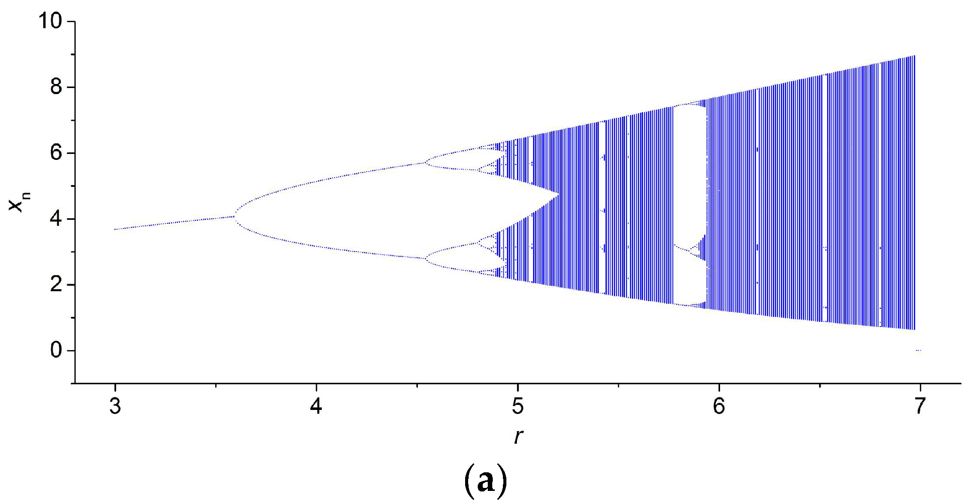
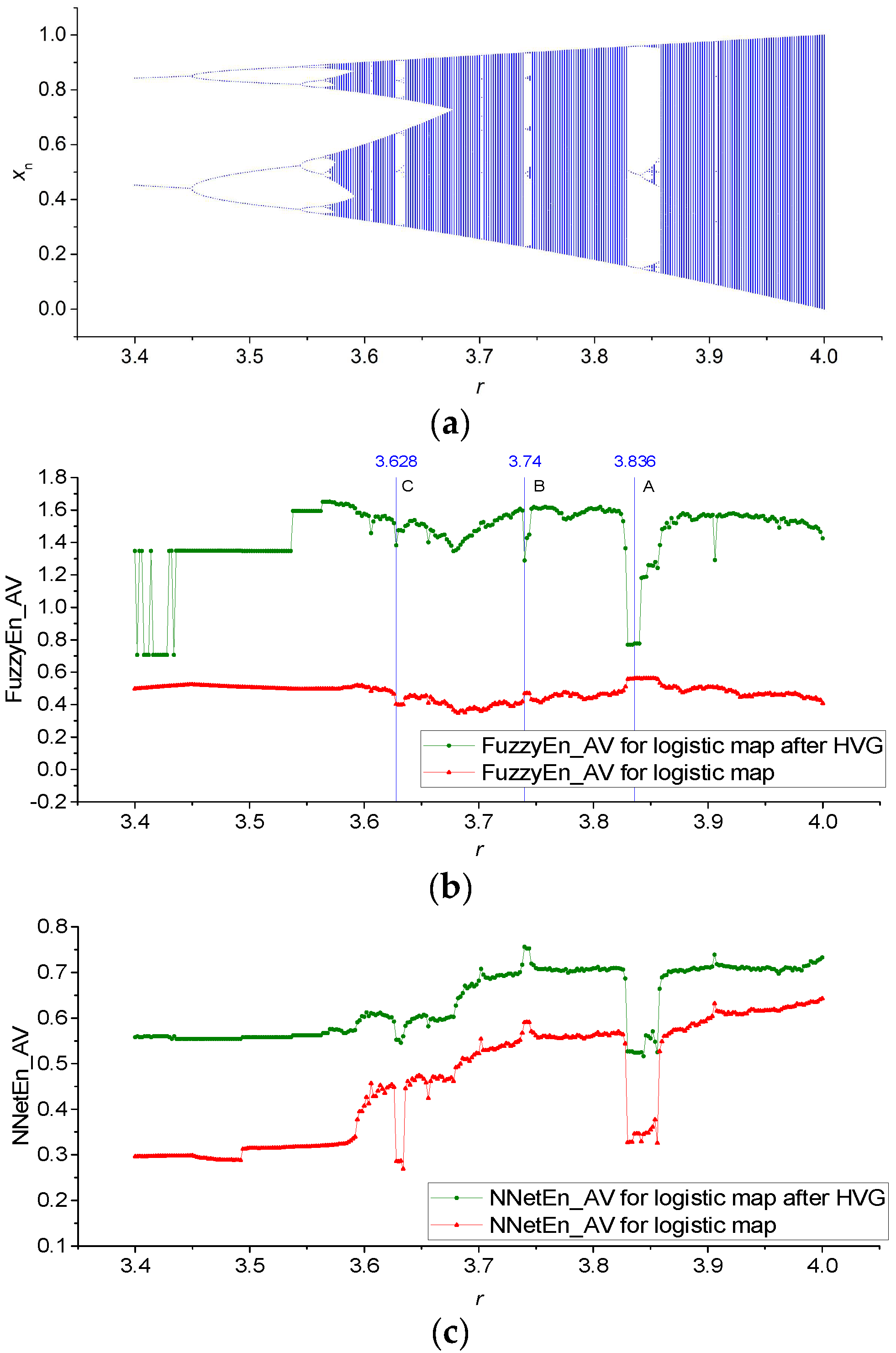
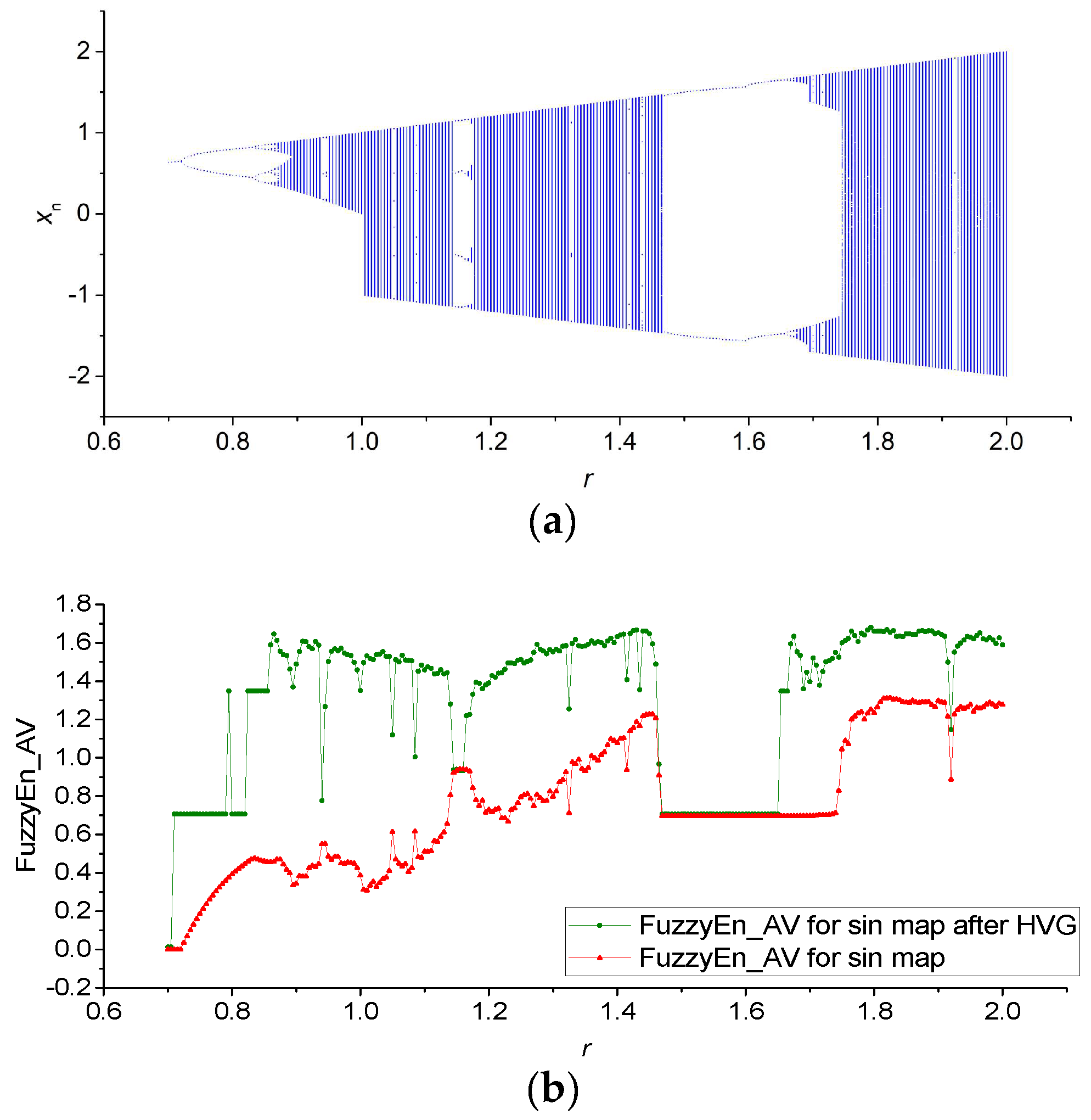
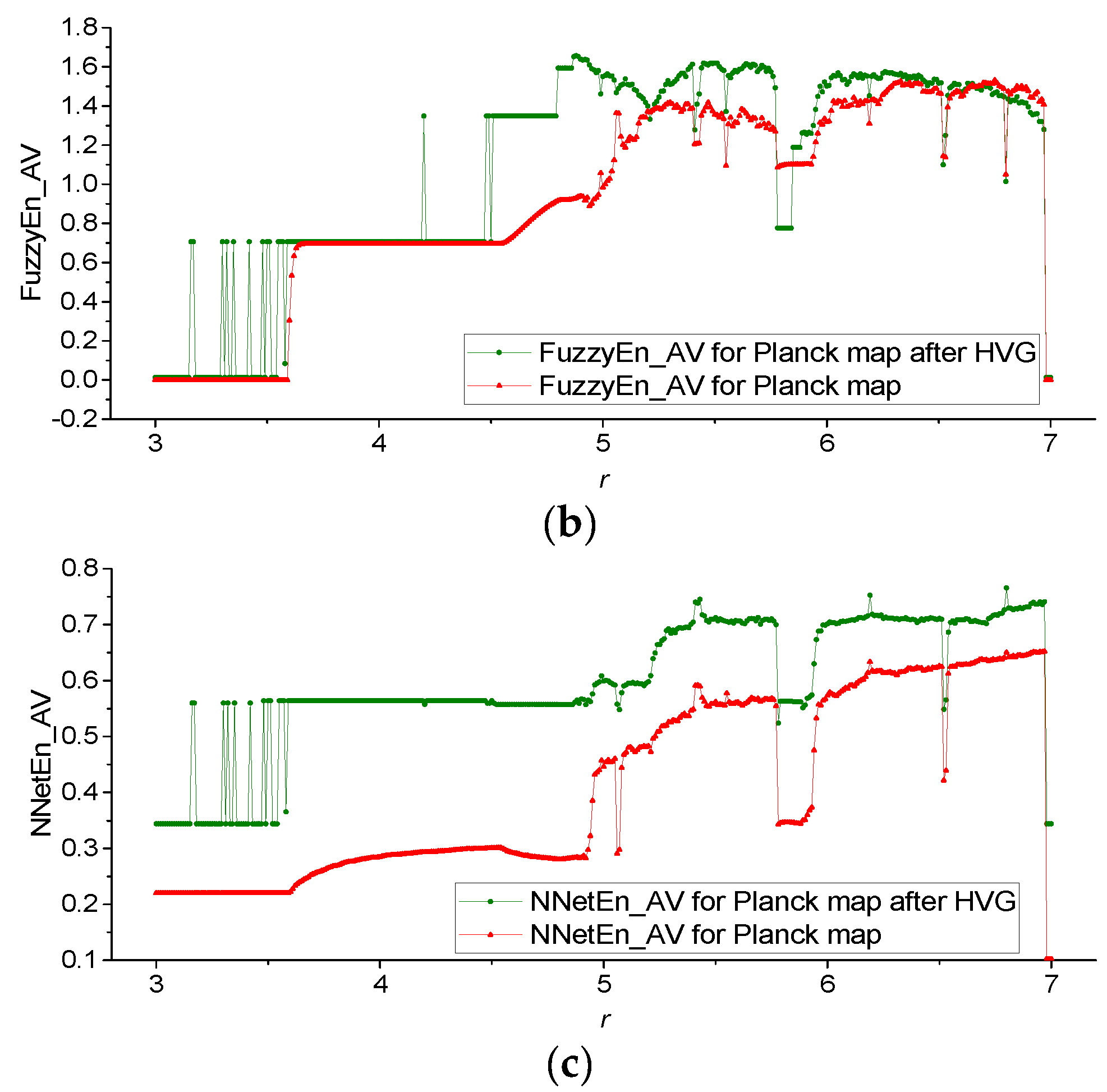
3.1. Results for Logistic, Sine, and Planck Maps

Figure 6a shows an example of a bifurcation diagram for a logistic map in the range of the control parameter 3.4 ≤ r ≤ 4, with a sampling step dr = 0.002. Figure 6b shows the FuzzyEn_AV(r) dependences before and after applying the HVG transformation. We can see that the HVG transformation significantly increases the entropy value, while some areas change their relative position. In regions A and B, we have reduced the entropies after having computed the HVGs, which is natural since they consist of ordered time series. The relative position of area C remained unchanged. The application of the HVG transformation had virtually no effect on the shape of the NNetEn_AV(r) graph, causing only a slight upward shift of entropies. The increase in FuzzyEn and NNetE values after HVG is due, in our opinion, to the fact that HVG has filtering properties and reduces the constant components of time series. However, FuzzyEn and NNetEn are sensitive to the constant component of the time series, which can be seen, for example, from the entropy values for r < 3.45.

Figure 7a presents the MCC(r) dependences for FuzzyEn before and after HVG transformation, as well as their difference in ΔMCC, which is computed as follows:

$$∆\mathrm{M}\mathrm{C}\mathrm{C}=\left|\mathrm{M}\mathrm{C}\mathrm{C} \mathrm{a}\mathrm{f}\mathrm{t}\mathrm{e}\mathrm{r} \mathrm{H}\mathrm{V}\mathrm{G}\right|-\left|\mathrm{M}\mathrm{C}\mathrm{C}\right|$$

(14)

Positive values of ΔMCC > 0 indicate that, for a given value of r, the degree of classification of time series for r_j−1 and r_j increases due to the HVG transformation. Conversely, negative ΔMCC values indicate a decrease in classification efficiency after HVG transformation. According to the lower figure (Figure 7, red line), the HVG transformation can lead to both an increase and a decrease in classification efficiency for different r_j. We provide detailed calculations of the GEFMCC values in

Table 1. Comparison of GEFMCC value for different chaotic mappings and entropies, before and after HVG. The average GEFMCC value for all chaotic mappings is given.

	GEFMCC				Average
	Logistic Map	Sine Map	Planck Map	TMBM Map	GEFMCC
FuzzyEn no HVG	0.572	0.524	0.360	0.539	0.499
FuzzyEn after HVG	0.334	0.362	0.355	0.2271	0.331
NNetEn no HVG	0.461	0.439	0.485	0.253	0.409
NNetEn after HVG	0.273	0.268	0.288	0.216	0.261

. The average GEFMCC values for all chaotic mappings are given.

Figure 7b shows the MCC(r) dependences for NeNetEn before and after HVG transformation and their difference in ΔMCC. It can be seen that the amplitude of MCC for FuzzyEn is more significant than for NNetEn, which also affects the GEFMCC value in Table 1.

It is convenient to compare the local values of MCC(r) for FuzzyEn and NeNetEn using their difference in ΔMCC (Figure 8).

$$\Delta \mathrm{MCC}=\left|\mathrm{MCC} \mathrm{for} \mathrm{NNetEn}\right|-\left|\mathrm{MCC} \mathrm{for} \mathrm{FuzzyEn}\right|$$

(15)

Figure 8 shows local areas of the time series dynamics in which the classification efficiency NNetEn is higher than FuzzyEn (ΔMCC > 0), but most of the graph shows ΔMCC < 0.

Similar results were obtained for the sine and Planck maps. Figure A1a (Appendix A) shows an example of a bifurcation diagram for a sine map in the control parameter range 0.7 ≤ r ≤ 2, with a sampling step dr = 0.005. Figure A1b,c show the FuzzyEn_AV(r) and NNetEn_AV(r) dependences before and after the application of the HVG transformation. Figure A2 shows the MCC(r) dependences for FuzzyEn and NNetEn before and after HVG transformation and their difference in ΔMCC.

Figure A3a (Appendix A) shows an example of a bifurcation diagram for a Planck map in the control parameter range 3 ≤ r ≤ 7, with a sampling step dr = 0.01. Figure A3b,c shows the FuzzyEn_AV(r) and NNetEn_AV(r) dependences before and after the application of the HVG transformation. Figure A4 shows the MCC(r) dependences for FuzzyEn and NNetEn before and after HVG transformation, and their difference in ΔMCC.

3.2. Results for TMBM Map

The TMBM map is multi-parametric and more complex than the mappings from Section 3.1. Figure 9a shows an example of a bifurcation diagram for a TMBM map in the control parameter range −1.7 ≤ r ≤ −1.5, with a sampling step dr = 0.0005.

After applying the HVG transformation, there is a notable increase in the entropy values of FuzzyEn_AV, as depicted in Figure 9b. Additionally, Figure 9c illustrates a consistent decrease in NNetEn_AV across a wide range of r following the utilization of HVF. Figure 10 shows the dependencies of MCC(r) and the discernible differences, denoted as ΔMCC, before and after the HVG transformation for both FuzzyEn (refer to Figure 10a) and NNetEn (refer to Figure 10b).

Figure 11 shows local areas of the time series dynamics in which the classification efficiency NNetEn is higher than FuzzyEn (ΔMCC > 0), but most of the graph shows ΔMCC < 0.

4. Discussion and Conclusions

In this work, we proposed a method for assessing the effectiveness of entropy features using chaotic mappings that enable the exploration of the efficiency of entropy-based classifications of time series.

Table 1 shows that FuzzyEn and NNetEn have a better GEFMCC performance without HVG transformation. This can be seen in the average GEFMCC values (last column of Table 1). At the same time, there were local areas of the time series dynamics where the classification efficiency of NNetEn was higher than that using FuzzyEn (Figure 8 and Figure 11). Nevertheless, despite reducing the amount of signal information after HVG transformations, there were local areas of time series dynamics where the classification efficiency increased when an HVG transformation was applied to the time series (Figure 7, Figure 10, Figure A2 and Figure A4). As seen in other contexts, HVGT transformations preserve the structural properties of the time series [33,34,35].

All chaotic mappings analyzed in this work presented a similar GEFMCC trend when applying HVGs and when comparing FuzzyEn and NNetEn. This indicates the universality of this characteristic phenomenon and the fundamentality of the results obtained. As a basic parameter when estimating entropy, we can take the average value of GEFMCC values over all chaotic mappings (last column of Table 1). It is necessary to consider that the results are given for specific entropy settings. Results may differ for other parameters since the entropies’ effectiveness depends on the entropy calculation parameters. For future research, different types of entropies can be compared under different parameters. In addition, it is interesting to identify the dependence of GEFMCC on the length of the time series. Further research should be conducted to explore other dynamical systems, as is the case for fractional dynamical systems based on the logistic and sine maps [54,55,56], where visibility graphs have already been considered [57].

Although we have shown that HVG representation generally reduces the classification ability of entropy-based features, it is possible to continue researching the influence of HVG transformation on the degree of classification of noisy signals by mixing weak noise into a time series of chaotic maps. This opens up additional research opportunities. The use of reference datasets based on chaotic mappings makes it possible to vary the length of the series in any range. In addition, it eliminates random, 1/f, or white noise, which is impossible to achieve in experimental databases that depend on experimental technology and the materials used.

We have shown the local effects of increasing the classification efficiency of individual time series when using NNetEn and HVG transformations. The finding contradicts the global trend measured by the GEFMCC parameter. In the case of entropy, this could be explained by the complexity of the entropy function that can be classified into individual dynamic modes, with a statistical spread from the average trend. In the case of HVG transformations, this explanation also applies. More research is needed into the effects of time series length and the effects of extraneous noise to see the complete picture of the effects.

The fact that FuzzyEn turned out to be more effective in classifying short (N = 300) time series than NNetEn confirmed the results of our work on the classification of EEG signals [1]. Moreover, experimental work [1,3] showed that FuzzyEn was the most effective compared to the other entropies, such as SampEn, SVDEn, and PermEn. However, individual pairs of time series can be better classified by NNetEn; this was also confirmed in the EEG experiment [1], where one channel performed better when using NNetEn as a feature. In the same works on EEG signals [1,3], the idea was put forward that classifications based on several features may perform better, and using FuzzyEn and NNetEn may lead to a synergistic effect.

The synergy effect of several entropies for signal classification can also be studied using our presented model of artificial databases based on chaotic mappings. To do this, it is necessary to replace the single feature threshold approach (Equation (6)) with a more complex classification model, for example, multi-layer perceptron or support vector classifiers. This may be a research direction for developing the GEFMCC entropy estimation approach presented in this work.

The technique we developed has a precise mathematical formulation and can be used to optimize entropy parameters, such in as the particle swarm optimization method. In this sense, the problem of classification based on entropy-based features has a more rigorous solution than assessing the magnitude of chaos and irregularity, which is often based on intuitive premises [58].

The entropy comparison method proposed in this work is helpful from a theoretical point of view and can be used in practice. Below, we show a comparison of the standard approach and its modification.

Previous approaches to analyzing EEG signals and choosing the type of entropy include the following:

(1)

Selecting measurement duration and sampling frequency of the EEG signal.

(2)

Experimenting to obtain a set of time series data.

(3)

Cutting time series using a specific length N. The value of N is often selected intuitively or through the repetition of similar work.

(4)

Selecting methods for processing time series, filter parameters, or wavelet transformations.

(5)

Selecting entropy characteristics, entropies, and their parameters, often intuitively, through the repetition of values from other works or by brute force.

The approach to analyzing EEG signals using the developed methodology included the following:

(1)

Finding the type of entropy and its parameters with the highest average GEFMCC value for four chaotic mappings (Table 1, last column). The search for the type of entropy and its parameters was carried out by enumeration or optimization using the particle swarm method. Optimize GEFMCC(N) for several values of time series length N. Select the minimum length N to correspond to the expected classification accuracy and the capabilities of the experiment.

(2)

Selecting the duration of measurements and sampling frequency of the EEG signal based on the analysis of the results of point 1.

(3)

Experimenting to obtain a set of time series data.

(4)

Cutting time series at a specific length N, based on the results of point 1.

(5)

Selecting methods for processing time series, filter parameters, or wavelet transformations.

(6)

Selecting entropy features, entropies, and their parameters, based on the results of point 1.

We chose four chaotic mappings (Section 2.2) because they all had different time series dynamics, and the TMBM had a complex multi-parameter function. Time series of any length can be reproducibly generated, while maintaining their inherent dynamics determined by the parameters of chaotic mappings. The stability of time series dynamics is difficult to reproduce in experimental data. Thus, artificial time series modeling is better suited for comparing entropies according to the GEFMCC efficiency criterion. Averaging the GEFMCC results over all mappings provides analytical results of the generalized entropy efficiency.

This method addresses the fundamental importance of finding a tool for comparing the effectiveness of entropies, which are used as features in classification problems. The developed technique can be applied to select entropy for EEG signals and to create Brain–Computer Interfacing and other applications for analyzing financial, biological, and medical signals.

References

- Velichko, A.; Belyaev, M.; Izotov, Y.; Murugappan, M.; Heidari, H. Neural Network Entropy (NNetEn): Entropy-Based EEG Signal and Chaotic Time Series Classification, Python Package for NNetEn Calculation. Algorithms 2023, 16, 255. [Google Scholar] [CrossRef]
- Aoki, Y.; Takahashi, R.; Suzuki, Y.; Pascual-Marqui, R.D.; Kito, Y.; Hikida, S.; Maruyama, K.; Hata, M.; Ishii, R.; Iwase, M.; et al. EEG Resting-State Networks in Alzheimer’s Disease Associated with Clinical Symptoms. Sci. Rep. 2023, 13, 3964. [Google Scholar] [CrossRef]
- Belyaev, M.; Murugappan, M.; Velichko, A.; Korzun, D. Entropy-Based Machine Learning Model for Fast Diagnosis and Monitoring of Parkinsons Disease. Sensors 2023, 23, 8609. [Google Scholar] [CrossRef]
- Yuvaraj, R.; Rajendra Acharya, U.; Hagiwara, Y. A Novel Parkinson’s Disease Diagnosis Index Using Higher-Order Spectra Features in EEG Signals. Neural Comput. Appl. 2018, 30, 1225–1235. [Google Scholar] [CrossRef]
- Aljalal, M.; Aldosari, S.A.; Molinas, M.; AlSharabi, K.; Alturki, F.A. Detection of Parkinson’s Disease from EEG Signals Using Discrete Wavelet Transform, Different Entropy Measures, and Machine Learning Techniques. Sci. Rep. 2022, 12, 22547. [Google Scholar] [CrossRef]
- Han, C.-X.; Wang, J.; Yi, G.-S.; Che, Y.-Q. Investigation of EEG Abnormalities in the Early Stage of Parkinson’s Disease. Cogn. Neurodyn. 2013, 7, 351–359. [Google Scholar] [CrossRef]
- Roy, G.; Bhoi, A.K.; Bhaumik, S. A Comparative Approach for MI-Based EEG Signals Classification Using Energy, Power and Entropy. IRBM 2022, 43, 434–446. [Google Scholar] [CrossRef]
- Cuesta-Frau, D.; Miró-Martínez, P.; Oltra-Crespo, S.; Jordán-Núñez, J.; Vargas, B.; González, P.; Varela-Entrecanales, M. Model Selection for Body Temperature Signal Classification Using Both Amplitude and Ordinality-Based Entropy Measures. Entropy 2018, 20, 853. [Google Scholar] [CrossRef]
- Vallejo, M.; Gallego, C.J.; Duque-Muñoz, L.; Delgado-Trejos, E. Neuromuscular Disease Detection by Neural Networks and Fuzzy Entropy on Time-Frequency Analysis of Electromyography Signals. Expert Syst. 2018, 35, e12274. [Google Scholar] [CrossRef]
- Nalband, S.; Prince, A.; Agrawal, A. Entropy-Based Feature Extraction and Classification of Vibroarthographic Signal Using Complete Ensemble Empirical Mode Decomposition with Adaptive Noise. IET Sci. Meas. Technol. 2018, 12, 350–359. [Google Scholar] [CrossRef]
- Wu, D.; Wang, X.; Su, J.; Tang, B.; Wu, S. A Labeling Method for Financial Time Series Prediction Based on Trends. Entropy 2020, 22, 1162. [Google Scholar] [CrossRef]
- Richman, J.S.; Moorman, J.R. Physiological Time-Series Analysis Using Approximate Entropy and Sample Entropy. Am. J. Physiol. Circ. Physiol. 2000, 278, H2039–H2049. [Google Scholar] [CrossRef]
- Chanwimalueang, T.; Mandic, D. Cosine Similarity Entropy: Self-Correlation-Based Complexity Analysis of Dynamical Systems. Entropy 2017, 19, 652. [Google Scholar] [CrossRef]
- Li, S.; Yang, M.; Li, C.; Cai, P. Analysis of Heart Rate Variability Based on Singular Value Decomposition Entropy. J. Shanghai Univ. 2008, 12, 433–437. [Google Scholar] [CrossRef]
- Xie, H.-B.; Chen, W.-T.; He, W.-X.; Liu, H. Complexity Analysis of the Biomedical Signal Using Fuzzy Entropy Measurement. Appl. Soft Comput. 2011, 11, 2871–2879. [Google Scholar] [CrossRef]
- Simons, S.; Espino, P.; Abásolo, D. Fuzzy Entropy Analysis of the Electroencephalogram in Patients with Alzheimer’s Disease: Is the Method Superior to Sample Entropy? Entropy 2018, 20, 21. [Google Scholar] [CrossRef]
- Mu, Z.; Hu, J.; Min, J. EEG-Based Person Authentication Using a Fuzzy Entropy-Related Approach with Two Electrodes. Entropy 2016, 18, 432. [Google Scholar] [CrossRef]
- Kumar, P.; Ganesan, R.A.; Sharma, K. Fuzzy Entropy as a Measure of EEG Complexity during Rajayoga Practice in Long-Term Meditators. In Proceedings of the 2020 IEEE 17th India Council International Conference (INDICON), New Delhi, India, 10–13 December 2020; pp. 1–5. [Google Scholar]
- Bandt, C.; Pompe, B. Permutation Entropy: A Natural Complexity Measure for Time Series. Phys. Rev. Lett. 2002, 88, 174102. [Google Scholar] [CrossRef]
- Chakraborty, S.; Paul, D.; Das, S. t-Entropy: A New Measure of Uncertainty with Some Applications. In Proceedings of the 2021 IEEE International Symposium on Information Theory (ISIT), Melbourne, Australia, 12–20 July 2021; pp. 1475–1480. [Google Scholar]
- Chen, Z.; Ma, X.; Fu, J.; Li, Y. Ensemble Improved Permutation Entropy: A New Approach for Time Series Analysis. Entropy 2023, 25, 1175. [Google Scholar] [CrossRef]
- LogNNet Neural Network|Encyclopedia MDPI. Available online: https://encyclopedia.pub/entry/2884 (accessed on 27 February 2024).
- Lecun, Y.; Bottou, L.; Bengio, Y.; Haffner, P. Gradient-Based Learning Applied to Document Recognition. Proc. IEEE 1998, 86, 2278–2324. [Google Scholar] [CrossRef]
- Xiong, J.; Liang, X.; Zhu, T.; Zhao, L.; Li, J.; Liu, C. A New Physically Meaningful Threshold of Sample Entropy for Detecting Cardiovascular Diseases. Entropy 2019, 21, 830. [Google Scholar] [CrossRef]
- Zhao, L.; Wei, S.; Zhang, C.; Zhang, Y.; Jiang, X.; Liu, F.; Liu, C. Determination of Sample Entropy and Fuzzy Measure Entropy Parameters for Distinguishing Congestive Heart Failure from Normal Sinus Rhythm Subjects. Entropy 2015, 17, 6270–6288. [Google Scholar] [CrossRef]
- Udhayakumar, R.K.; Karmakar, C.; Li, P.; Palaniswami, M. Effect of Embedding Dimension on Complexity Measures in Identifying Arrhythmia. In Proceedings of the 2016 38th Annual International Conference of the IEEE Engineering in Medicine and Biology Society (EMBC), Orlando, FL, USA, 16–20 August 2016; pp. 6230–6233. [Google Scholar]
- Myers, A.; Khasawneh, F.A. On the Automatic Parameter Selection for Permutation Entropy. Chaos Interdiscip. J. Nonlinear Sci. 2020, 30, 33130. [Google Scholar] [CrossRef]
- Cuesta-Frau, D.; Murillo-Escobar, J.P.; Orrego, D.A.; Delgado-Trejos, E. Embedded Dimension and Time Series Length. Practical Influence on Permutation Entropy and Its Applications. Entropy 2019, 21, 385. [Google Scholar] [CrossRef]
- EntropyHub/EntropyHub Guide.Pdf at Main MattWillFlood/EntropyHub GitHub. Available online: https://github.com/MattWillFlood/EntropyHub/blob/main/EntropyHubGuide.pdf (accessed on 14 March 2024).
- Flood, M.W.; Grimm, B. EntropyHub: An Open-Source Toolkit for Entropic Time Series Analysis. PLoS ONE 2021, 16, e0259448. [Google Scholar] [CrossRef]
- Ribeiro, M.; Henriques, T.; Castro, L.; Souto, A.; Antunes, L.; Costa-Santos, C.; Teixeira, A. The Entropy Universe. Entropy 2021, 23, 222. [Google Scholar] [CrossRef]
- Lacasa, L.; Luque, B.; Ballesteros, F.; Luque, J.; Nuño, J.C. From Time Series to Complex Networks: The Visibility Graph. Proc. Natl. Acad. Sci. USA 2008, 105, 4972–4975. [Google Scholar] [CrossRef]
- Lacasa, L.; Toral, R. Description of Stochastic and Chaotic Series Using Visibility Graphs. Phys. Rev. E 2010, 82, 36120. [Google Scholar] [CrossRef]
- Luque, B.; Lacasa, L.; Ballesteros, F.J.; Robledo, A. Feigenbaum Graphs: A Complex Network Perspective of Chaos. PLoS ONE 2011, 6, e22411. [Google Scholar] [CrossRef]
- Flanagan, R.; Lacasa, L.; Nicosia, V. On the Spectral Properties of Feigenbaum Graphs. J. Phys. A Math. Theor. 2019, 53, 025702. [Google Scholar] [CrossRef]
- Requena, B.; Cassani, G.; Tagliabue, J.; Greco, C.; Lacasa, L. Shopper Intent Prediction from Clickstream E-Commerce Data with Minimal Browsing Information. Sci. Rep. 2020, 10, 16983. [Google Scholar] [CrossRef]
- Casado Vara, R.; Li, L.; Iglesias Perez, S.; Criado, R. Increasing the Effectiveness of Network Intrusion Detection Systems (NIDSs) by Using Multiplex Networks and Visibility Graphs. Mathematics 2022, 11, 107. [Google Scholar] [CrossRef]
- Akgüller, Ö.; Balcı, M.A.; Batrancea, L.M.; Gaban, L. Path-Based Visibility Graph Kernel and Application for the Borsa Istanbul Stock Network. Mathematics 2023, 11, 1528. [Google Scholar] [CrossRef]
- Li, S.; Shang, P. Analysis of Nonlinear Time Series Using Discrete Generalized Past Entropy Based on Amplitude Difference Distribution of Horizontal Visibility Graph. Chaos Solitons Fractals 2021, 144, 110687. [Google Scholar] [CrossRef]
- Hu, X.; Niu, M. Degree Distributions and Motif Profiles of Thue–Morse Complex Network. Chaos Solitons Fractals 2023, 176, 114141. [Google Scholar] [CrossRef]
- Gao, M.; Ge, R. Mapping Time Series into Signed Networks via Horizontal Visibility Graph. Phys. A Stat. Mech. Its Appl. 2024, 633, 129404. [Google Scholar] [CrossRef]
- Li, S.; Shang, P. A New Complexity Measure: Modified Discrete Generalized Past Entropy Based on Grain Exponent. Chaos Solitons Fractals 2022, 157, 111928. [Google Scholar] [CrossRef]
- May, R.M. Simple Mathematical Models with Very Complicated Dynamics. Nature 1976, 261, 459–467. [Google Scholar] [CrossRef]
- Sedik, A.; El-Latif, A.A.A.; Wani, M.A.; El-Samie, F.E.A.; Bauomy, N.A.; Hashad, F.G. Efficient Multi-Biometric Secure-Storage Scheme Based on Deep Learning and Crypto-Mapping Techniques. Mathematics 2023, 11, 703. [Google Scholar] [CrossRef]
- Velichko, A.; Heidari, H. A Method for Estimating the Entropy of Time Series Using Artificial Neural Networks. Entropy 2021, 23, 1432. [Google Scholar] [CrossRef]
- Pham, V.-T.; Velichko, A.; Van Huynh, V.; Radogna, A.V.; Grassi, G.; Boulaaras, S.M.; Momani, S. Analysis of Memristive Maps with Asymmetry. Integration 2024, 94, 102110. [Google Scholar] [CrossRef]
- Carlos Bergillos Varela Ts2vg. Available online: https://pypi.org/project/ts2vg/ (accessed on 27 February 2024).
- Chen, W.; Wang, Z.; Xie, H.; Yu, W. Characterization of Surface EMG Signal Based on Fuzzy Entropy. IEEE Trans. Neural Syst. Rehabil. Eng. 2007, 15, 266–272. [Google Scholar] [CrossRef]
- EntropyHub. An Open-Source Toolkit for Entropic Time Series Analysis. Available online: https://www.entropyhub.xyz/ (accessed on 27 February 2024).
- NNetEn Entropy|Encyclopedia MDPI. Available online: https://encyclopedia.pub/entry/18173 (accessed on 27 February 2024).
- MNIST Handwritten Digit Database, Yann LeCun, Corinna Cortes and Chris Burges. Available online: http://yann.lecun.com/exdb/mnist/ (accessed on 16 August 2020).
- GitHub—Izotov93/NNetEn: Python Package for NNetEn Calculation. Available online: https://github.com/izotov93/NNetEn (accessed on 15 February 2024).
- Chicco, D.; Warrens, M.J.; Jurman, G. The Matthews Correlation Coefficient (MCC) Is More Informative than Cohen’s Kappa and Brier Score in Binary Classification Assessment. IEEE Access 2021, 9, 78368–78381. [Google Scholar] [CrossRef]
- Wu, G.C.; Baleanu, D. Discrete Fractional Logistic Map and Its Chaos. Nonlinear Dyn. 2014, 75, 283–287. [Google Scholar] [CrossRef]
- Wu, G.C.; Niyazi Cankaya, M.; Banerjee, S. Fractional Q-Deformed Chaotic Maps: A Weight Function Approach. Chaos 2020, 30, 121106. [Google Scholar] [CrossRef] [PubMed]
- Wu, G.C.; Baleanu, D.; Zeng, S. Da Discrete Chaos in Fractional Sine and Standard Maps. Phys. Lett. A 2014, 378, 484–487. [Google Scholar] [CrossRef]
- Conejero, J.A.; Lizama, C.; Mira-Iglesias, A.; Rodero, C. Visibility Graphs of Fractional Wu–Baleanu Time Series. J. Differ. Equations Appl. 2019, 25, 1321–1331. [Google Scholar] [CrossRef]
- Xiao, H.; Mandic, D.P. Variational Embedding Multiscale Sample Entropy: A Tool for Complexity Analysis of Multichannel Systems. Entropy 2022, 24, 26. [Google Scholar] [CrossRef] [PubMed]