A Risk-Structured Model for the Transmission Dynamics of Anthrax Disease

Abstract

Anthrax, a zoonotic disease with serious public health consequences, has been the subject of rigorous mathematical and statistical modeling to better understand its dynamics and to devise effective control techniques. In this study, we propose a novel mathematical risk-structured model for anthrax disease spread that includes both qualitative and quantitative evaluations. Our research focuses on the complex interplay between host–anthrax interactions and zoonotic transmission. Our mathematical approach incorporates bifurcation analysis and stability considerations. We investigate the dynamic behavior of the proposed model under various settings, shedding light on the important parameters that determine anthrax transmission and persistence. The normalized forward sensitivity analysis method is used to determine the parameters that are relevant to reducing ${\mathcal{R}}_c$ and, by extension, disease spread. Through scenario simulation of our model, we identify intervention techniques, such as enlightenment of the populace, that will effectively minimize disease transmission. Our findings provide insights into anthrax epidemiology and emphasize the importance of effective disease management. Bifurcation investigations reveal the existence and stability of numerous equilibria, allowing for a better understanding of the behavior of the system under various scenarios. This study adds to the field of anthrax modeling by providing a foundation for informed decision-making regarding public health measures. The use of a mathematical modeling approach improves our ability to anticipate and control anthrax epidemics, ultimately helping to protect both human and animal populations.

1. Introduction

Anthrax is caused by the bacterium Bacillus anthracis [1] and is a serious infectious disease that affects both humans and animals worldwide. It is primarily transmitted to hosts through the ingestion of contaminated feed or water sources, inhalation of airborne spores, or penetration via damaged skin. Once inside the body, spores germinate and spread to internal organs [2], leading to the manifestation of the disease, which can be fatal [3,4].

Anthrax is found worldwide, with certain regions, particularly in Asia and Africa [5], considered to be the main reservoirs of the disease. Human and animal interactions as well as climatic factors influenced by climate change contribute to the spread of anthrax and other infectious diseases.

Climate change is recognized as a major driver of emerging infectious diseases, including anthrax. Changes in temperature, precipitation patterns, and ecological conditions can affect the distribution and prevalence of anthrax, thereby increasing the risk to vulnerable populations [6,7].

Early detection and prevention programs are crucial for mitigating the threat of anthrax and other emerging infectious diseases. Vaccination of animals, surveillance of high-risk areas, and public health interventions to educate communities about preventive measures are essential strategies to reduce the burden of anthrax.

While anthrax may not be considered among the most pressing public health concerns globally, its potential for severe illness and fatality underscores the importance of effective prevention and control measures. Given the threat of climate change and the interconnectedness of human and animal health, proactive efforts to monitor, prevent, and respond to anthrax outbreaks are critical for safeguarding public health and mitigating the impacts of emerging infectious diseases.

Mathematical and statistical models have been developed to study the transmission dynamics of anthrax disease and have used several methodological approaches to understand its spread in several countries [8]. Some of these methodological approaches have also been used to study the transmission of Mpox disease by the authors in [9], Zika and Dengue viruses in [10], and most recently, the highly contagious COVID-19 epidemic that was experienced globally in [11]. We will attempt to review some of the articles in this research direction and will state some of the gaps in the literature and our contribution to the modeling of anthrax disease dynamics.

A systematic review and evaluation of mathematical models of human inhalation anthrax for supporting public health policymaking, response, and proper deployment of adequate resources were studied in [12]. In [13]; the mathematical modeling framework presented to study anthrax dynamics incorporated novel components such as fast and slow progression, carcass disposal, and a vector population. This research presented some mathematical analyses and simulations that enabled the authors to suggest that appropriate carcass disposal may significantly reduce the spread of anthrax. A mathematical model to study anthrax transmission dynamics in animal populations, excluding the human population, was studied in [14]. The research presented a general anthrax disease model with sub-models for two categories of animals: that is, herbivore and carnivore models. It was shown using numerical simulations and by way of seasonal variations due to various environmental factors, such as cycles of heavy rainfall followed by periods of dry weather, that oscillations in spore growth may drive oscillations in animal population dynamics. However, the total number of infected animals remained constant, similar to spore growth. Because climate change is one of the most significant factors contributing to the transmission of anthrax disease, the research presented in [15] used Kenya as a case study to evaluate the potential future distribution of anthrax outbreaks under multiple climate change scenarios. This research proposed a prediction of the potential anthrax distribution under changing climates that can inform anticipatory measures to prevent future anthrax risk.

In [16], a mathematical model to study anthrax transmission in both human and animal populations was presented. The advantage of the model developed by the authors over the existing models was that it compared the rates of infection and the rates of recovery from anthrax disease in both human and animal populations, which was validated by the numerical simulation results presented in the article. In [17], computer methods were used to study a compartmental model developed for anthrax transmissions. In [8,18], the authors developed a mathematical model to study behavioral changes during an anthrax outbreak; optimal control and cost-effectiveness analyses were performed on the anthrax epidemic model. In [19], a compartmental model was developed to understand how environmental and host population dynamics affect anthrax outbreaks. The authors found that disease transmission was influenced more by the seasonality of environmental factors than by the animal population. The authors in [20] developed deterministic models that incorporated a vaccination compartment. Their study revealed that anthrax transmission within an animal population can be controlled by implementing vaccination policies. Other models developed in the literature by different researchers to study anthrax disease transmission dynamics using several case studies and control measures can be found in [21,22,23,24,25]. Through our study, we aim to make significant contributions to the existing literature on this topic by providing valuable insights into the mathematical modeling of anthrax disease in human and animal populations. The main objective is to investigate the influence of some of the introduced model variables and parameters on the dynamics of the disease and to analyze the model qualitatively and quantitatively. The scenarios presented offer better insights into anthrax disease modeling. Available datasets recorded for anthrax disease are sparse; however, we validate the theoretical aspect of our work using case–scenario numerical simulations.

In this research, we develop a mathematical model that explores risk exposure levels for individuals and incorporates the loss of infection-acquired immunity by both populations and the release of pathogens into the environment by both infected animals and carcasses of dead infected animals. This brings novelty to the work presented in this study; hence, it is an extension of existing dynamical models for anthrax disease transmission. We present some qualitative analyses of the model we developed and explore some scenarios and simulations of the model.

The rest of the paper is organized as follows: The mathematical model formulation is presented in Section 2, while the model analyses are carried out in Section 3. In Section 4, parameterization of the model, sensitivity analysis of the model threshold parameter, scenario simulations, and interpretation and discussion of the results are presented. In Section 5, we present our concluding remarks, limitations, and future work.

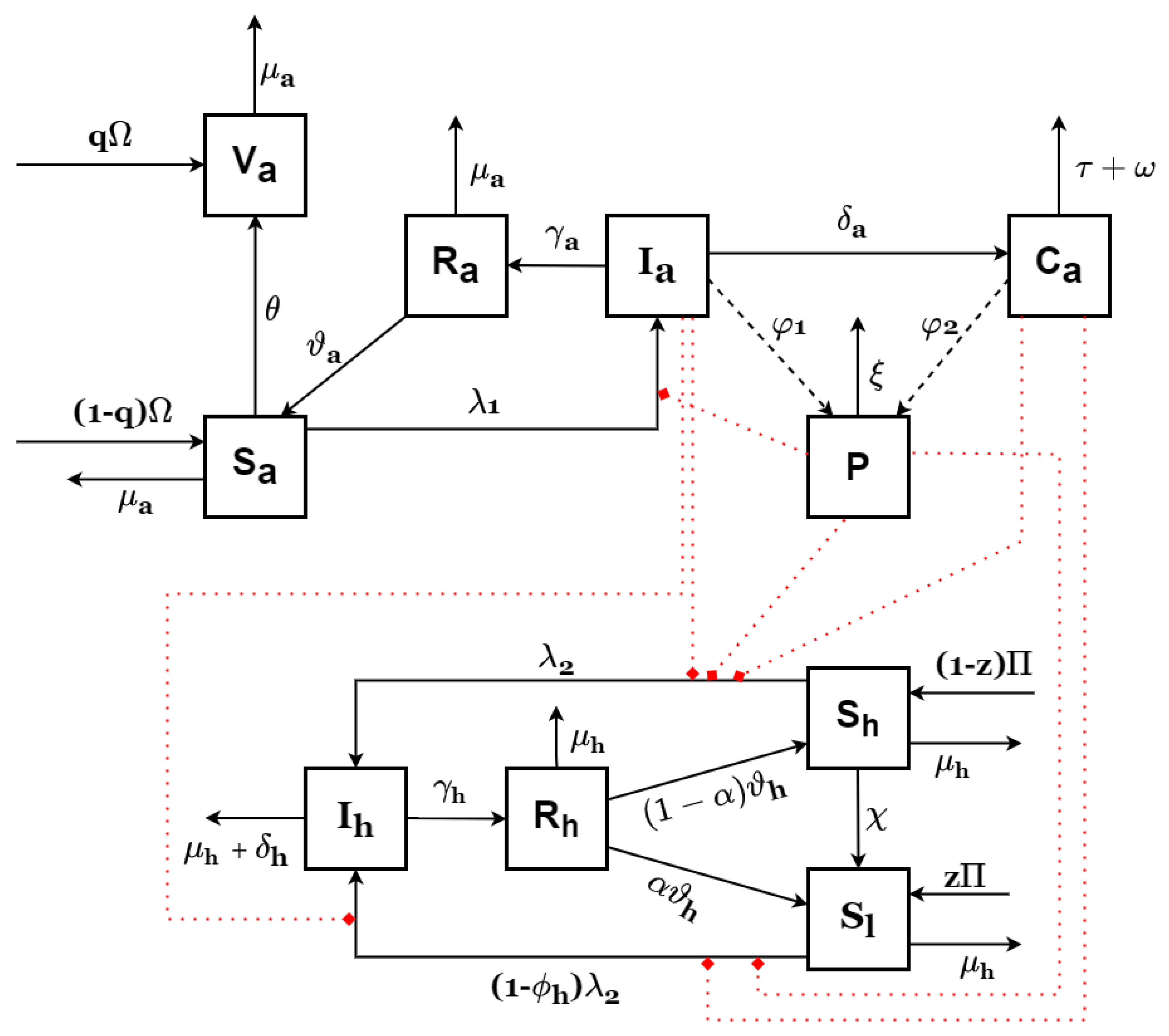
2. Model Formulation

In this study, we considered both animal and human populations. The total human population $N_h$ is subdivided into four compartments: individuals at high risk of contracting anthrax disease $S_h$, individuals at a reduced risk of contracting the anthrax disease $S_l$, the population of individuals infected with the disease $I_h$, and those who have recovered from the disease $R_h$. The total animal population $N_a$ is divided into five compartments: susceptible animals $S_a$, vaccinated animals $V_a$, infected animals $I_a$, recovered animals $R_a$, and animals (carcass) that died from the disease $C_a$. The density of the Bacillus anthracis virus in the population environment is denoted by P. Summarily,

$$N_h=S_h+S_l+I_h+R_h\mathrm{and}{N}_a=S_a+V_a+I_a+R_a+C_a$$

The following assumptions were made when designing the model:

• There is no vertical transmission in both populations.
• High-risk susceptibles can become low-risk susceptibles due to their adoption of protective measures as a result of educational and enlightenment campaigns.
• A fraction of the recruited animals are effectively vaccinated.
• Susceptible humans and animals get infected by coming into contact with infected livestock, infected carcasses, and spores.
• There is no human-to-human infection.
• Recovered humans and animals can lose infection-acquired immunity.
• Animal vaccination is perfect.
• Only healthy animals are recruited into the population.

The total susceptible human population is increased by recruitment at a constant rate $\mathsf{\Pi }$. A portion z of these recruited individuals is at low risk of contracting the disease, while the rest are at high risk. The population of susceptible high-risk individuals also increases when recovered individuals lose their infection-acquired immunity at the rate ${\vartheta }_h$ and become highly susceptible again. Education/enlightenment efforts, when adopted by these high-risk individuals, reduce their risk and susceptibility to the disease, thereby reducing their population at a rate of $\chi$. Infection with the anthrax disease from infected animals, carcasses, and the environment at a rate of ${\beta }_2$ and death due to natural causes at the rate of ${\mu }_h$ further diminish this population. Thus, the disease dynamics for high-risk susceptible individuals are given by

$$\frac{d{S}_h}{dt}=(1-z)\mathsf{\Pi }-\chi S_h-{\lambda }_2{S}_h-{\mu }_h{S}_h+(1-\alpha ){\vartheta }_h{R}_h.$$

For low-risk susceptible individuals $S_l$, their population increases with enlightenment and subsequent behavioral changes due to high-risk susceptibility and loss of infection-acquired immunity by recovered individuals. It is decreased by death due to other causes and infection with the disease at the rate $(1-{\varphi }_h){\beta }_2$, where ${\varphi }_h$ is a modification parameter representing the behavioral dispositions adopted by these low-risk susceptibles to ensure that they are significantly shielded from contracting anthrax disease. This is mathematically expressed as

$$\frac{d{S}_l}{dt}=z\mathsf{\Pi }+\chi S_h-(1-{\varphi }_h){\lambda }_2{S}_l-{\mu }_h{S}_l+\alpha {\vartheta }_h{R}_h.$$

The description follows for infected humans $I_h$ and recovered humans $R_h$. For the animal population, there is constant recruitment at the rate $\mathsf{\Omega }$, where a portion of these animals $(1-q)$ is fully susceptible to the disease $S_a$, while the remaining fraction q enters the population already vaccinated $V_a$. The susceptible animal population further increases when the immunity of recovered animals wanes at the rate ${\vartheta }_a$. Infection with anthrax disease from carcasses and environmental spores at the rate of ${\beta }_1$, effective animal vaccination at the rate of $\theta$, and death from other causes all serve to reduce the population of susceptible animals. Epidemiologically, we write this as

$$\frac{d{S}_a}{dt}=(1-q)\mathsf{\Omega }-{\lambda }_1{S}_a-\theta S_a-{\mu }_a{S}_a+{\vartheta }_a{R}_a.$$

When animals die from anthrax, their carcasses populate the $C_a$ compartment. These carcasses release Bacillus anthracis spores into the soil and environment at the rate $\omega$ as they decay. Scavengers consume these carcasses at the rate $\tau$, further reducing the number of carcasses and becoming infected during the process. This is represented as

$$\frac{d{C}_a}{dt}={\delta }_a{I}_a-(\tau +\omega )C_a.$$

Infected animals release pathogens of the Bacillus anthracis virus into the environment at the rate ${\phi }_1$, whereas decaying carcasses do the same at the rate ${\phi }_2$. Both activities increase the density of the pathogen in the environment, while the pathogens are removed at a rate of $\xi$. Hence, pathogen density dynamics in the environment are given by

$$\frac{dP}{dt}={\phi }_1{I}_a+{\phi }_2{C}_a-\xi P.$$

The transition description for the other compartments follows Equation (1). In general, the model formulated for this research is represented by Equation (1), and the parameters and variables are listed in

Table 1. Description of model variables and parameters.

Variable	Interpretation
$S_a$	Population of susceptible animals
$V_a$	Population of vaccinated animals
$I_a$	Population of infected animals
$R_a$	Population of recovered animals
$C_a$	Carcasses of dead animals
P	Environmental spore density of Bacillus anthracis
$S_h$	Population of susceptible high-risk individuals
$S_l$	Population of susceptible low-risk individuals
$I_h$	Population of infected individuals
$R_h$	Population of recovered individuals
Parameter	Interpretation
$\mathsf{\Omega },\mathsf{\Pi }$	Recruitment rates into animal and human populations, respectively
${\beta }_1,{\beta }_2$	Effective disease transmission rate for animals and humans, respectively
$\theta$	Effective vaccination rate of animals
$\alpha$	Proportion of recovered individuals that become low-risk susceptibles
z	Fraction of recruited humans categorized to be low-risk
q	Fraction of recruited animals that come into the population already vaccinated
$\tau$	Rate of carcass consumption by scavengers
$\omega$	Natural decomposition rate of carcasses
${\varphi }_h$	Modification parameter for behavioral dispositions of low-risk susceptibles
$\chi$	Enlightenment/educational campaign efforts at controlling the disease
$\xi$	Removal/natural decay rate of spores
${\phi }_1,{\phi }_2$	Pathogen release rate from infected animals and decaying carcasses, respectively
${\gamma }_h,{\gamma }_a$	Recovery rate for humans and animals, respectively
${\mu }_h,{\mu }_a$	Natural death rates of humans and animals
${\delta }_h,{\delta }_a$	Disease-induced death rates for humans and animals, respectively
${\vartheta }_h,{\vartheta }_a$	Rate of loss of infection-acquired immunity by individuals and animals, respectively

. A schematic diagram of the proposed model is shown in Figure 1.

$$\begin{array}{c}\frac{d{S}_a}{dt}=(1-q)\mathsf{\Omega }-{\lambda }_1{S}_a-\theta S_a-{\mu }_a{S}_a+{\vartheta }_a{R}_a,\hfill \\ \frac{d{V}_a}{dt}=q\mathsf{\Omega }+\theta S_a-{\mu }_a{V}_a,\hfill \\ \frac{d{I}_a}{dt}={\lambda }_1{S}_a-({\gamma }_a+{\mu }_a+{\delta }_a)I_a,\hfill \\ \frac{d{R}_a}{dt}={\gamma }_a{I}_a-{\mu }_a{R}_a-{\vartheta }_a{R}_a,\hfill \\ \frac{d{C}_a}{dt}={\delta }_a{I}_a-(\tau +\omega )C_a,\hfill \\ \frac{dP}{dt}={\phi }_1{I}_a+{\phi }_2{C}_a-\xi P,\hfill \\ \frac{d{S}_h}{dt}=(1-z)\mathsf{\Pi }-\chi S_h-{\lambda }_2{S}_h-{\mu }_h{S}_h+(1-\alpha ){\vartheta }_h{R}_h,\hfill \\ \frac{d{S}_l}{dt}=z\mathsf{\Pi }+\chi S_h-(1-{\varphi }_h){\lambda }_2{S}_l-{\mu }_h{S}_l+\alpha {\vartheta }_h{R}_h,\hfill \\ \frac{d{I}_h}{dt}={\lambda }_2{S}_h+(1-{\varphi }_h){\lambda }_2{S}_l-({\gamma }_h+{\mu }_h+{\delta }_h)I_h,\hfill \\ \frac{d{R}_h}{dt}={\gamma }_h{I}_h-{\mu }_h{R}_h-{\vartheta }_h{R}_h,\hfill \end{array}$$

(1)

where:

$${\lambda }_1={\beta }_1(C_a+P),{\lambda }_2={\beta }_2({\displaystyle \frac{I_a}{N_a}}+C_a+P).$$

3. Analyses of the Model

In this section, some qualitative analyses of the model are performed. Firstly, we demonstrate two basic properties of the model, which are the invariant region (depicting the domain in which the solution of the model makes sense mathematically and epidemiologically) and the non-negativity of the model solution. After these, we proceed to more rigorous investigations such as the existence and uniqueness of the model solution, analysis of the model equilibria, the basic reproduction number, bifurcation analysis, and global stability analysis.

3.1. Boundedness of Solutions

Theorem 1.

The closed set

$$\mathcal{D}={\mathcal{D}}_h\times {\mathcal{D}}_a\times {\mathcal{D}}_p$$

(2)

with ${\mathcal{D}}_h=\left\{S_h,S_l,I_h,R_h\in {\mathcal{R}}_{+}^4:N_h\le \frac{\mathsf{\Pi }}{{\mu }_h}\right\}$, ${\mathcal{D}}_a=\left\{S_a,V_a,I_a,R_a,C_a\in {\mathcal{R}}_{+}^5:N_a\le \frac{\mathsf{\Omega }}{{\mu }_a}\right\}$ and ${\mathcal{D}}_p=\left\{P\in {\mathcal{R}}_{+}^1\right\}$ is positively invariant with respect to the model (1).

Proof. 

The total animal population is denoted by $N_a$ and given by $N_a(t)=S_a(t)+V_a(t)+I_a(t)+R_a(t)+C_a(t)$ and is differentiated and summed together to obtain

$$\frac{d{N}_a}{dt}=\mathsf{\Omega }-{\mu }_a{N}_a-(\tau +\omega -{\mu }_a)C_a.$$

(3)

But ${\mu }_a{C}_a=0$, so that by standard comparison and rearranging Equation (3), we obtain a first-order differential inequality:

$$\frac{d{N}_a}{dt}+{\mu }_a{N}_a\le \mathsf{\Omega },$$

which we solve by the integrating factor method to obtain

$$N_a(t)\le \frac{\mathsf{\Omega }}{{\mu }_a}\left(1-e^{-{\mu }_{a}t}\right)+N_a(0)e^{-{\mu }_{a}t},$$

(4)

as $t\to \infty$,

$$N_a(t)\le \frac{\mathsf{\Omega }}{{\mu }_a}.$$

(5)

□

Following a similar approach yields a similar result for the human population: $N_h(t)\le \frac{\mathsf{\Pi }}{{\mu }_h}$. Thus, we have shown that $\mathcal{D}$ is positively invariant and attracts all solutions of Equation (1) in finite time. This guarantees that our investigations and analyses will be carried out in a feasible region and that every solution of our model having initial conditions in $\mathcal{D}$ will always remain in $\mathcal{D}$ for all $t>0$.

3.2. Non-Negativity of Solutions

Next, we establish that every solution of the model Equation (1) will be non-negative for all time t.

Theorem 2.

Let $(S_a(0),V_a(0),I_a(0),R_a(0),C_a(0),P(0),S_h(0),S_l(0),I_h(0),R_h(0))\ge 0$ be the initial states of the model (1). Then every solution $(S_a(t),V_a(t),I_a(t),R_a(t),C_a(t),P(t),S_h(t),$$S_l(t),I_h(t),R_h(t))\ge 0$ for all time $t>0$.

Proof. 

From the first equation of our model (1),

$$\frac{d{S}_a}{dt}=(1-q)\mathsf{\Omega }-{\lambda }_1{S}_a-\theta S_a-{\mu }_a{S}_a+{\vartheta }_a{R}_a.$$

So by collecting like terms, we have

$$\frac{d{S}_a}{dt}+({\lambda }_1+\theta +{\mu }_a)S_a=(1-q)\mathsf{\Omega }+{\vartheta }_a{R}_a$$

and

$$\frac{d{S}_a}{dt}+({\lambda }_1+\theta +{\mu }_a)S_a\ge (1-q)\mathsf{\Omega }.$$

(6)

Solving Equation (6) by using the integrating factor method gives

$$\begin{array}{ccc}\hfill \frac{d}{dt}\left[S_{a}exp\{(\theta +{\mu }_a)t+{\int }_0^t{\lambda }_1(\rho )d\rho \}\right]& \ge & (1-q)\mathsf{\Omega }exp\{(\theta +{\mu }_a)t+{\int }_0^t{\lambda }_1(\rho )d\rho \}\hfill \\ \hfill {\int }_0^{t_f}\left(\frac{d}{dt}\left[S_{a}exp\{(\theta +{\mu }_a)t+{\int }_0^t{\lambda }_1(\rho )d\rho \}\right]\right)& \ge & {\int }_0^{t_f}\left((1-q)\mathsf{\Omega }exp\{(\theta +{\mu }_a)t+{\int }_0^t{\lambda }_1(\rho )d\rho \}\right),\hfill \end{array}$$

Hence,

$$\begin{array}{ccc}\hfill S_a(t_f)\left[exp\{(\theta +{\mu }_a)t_f+{\int }_0^{t_f}{\lambda }_1(\rho )d\rho \}\right]-S_a(0)& \ge & (1-q)\mathsf{\Omega }{\int }_0^{t_f}\left[exp\{(\theta +{\mu }_a)y+{\int }_0^y{\lambda }_1(\rho )d\rho \}\right]dy,\hfill \end{array}$$

so that

$$\begin{array}{ccc}\hfill S_a(t_f)& \ge & S_a(0)exp\left[-\{(\theta +{\mu }_a)t_f+{\int }_0^{t_f}{\lambda }_1(\rho )d\rho \}\right]\hfill \\ & +& exp\left[-\{(\theta +{\mu }_a)t_f+{\int }_0^{t_f}{\lambda }_1(\rho )d\rho \}\right]\times (1-q)\mathsf{\Omega }{\int }_0^{t_f}\left[exp\{(\theta +{\mu }_a)y+{\int }_0^y{\lambda }_1(\rho )d\rho \}\right]dy.\hfill \end{array}$$

(7)

But $S_a(0)>0$ for $t>0$ $\Rightarrow S_a(t_f)\ge 0$. □

Therefore, any solution of $S_a$ with non-negative initial data will remain non-negative $\forall t>0$. In the same manner, it can be shown that $V_a(t)\ge 0,I_a(t)\ge 0,R_a(t)\ge 0,C_a(t)\ge 0,P(t)\ge 0,S_h(t)\ge 0,S_l(t)\ge 0,I_h(t)\ge 0,R_h(t)\ge 0$.

3.3. Existence and Uniqueness of the Solution

Theorem 3.

The model (1) defined by ${\mathbb{R}}_{+}^{10}\in \mathcal{D}$ of (2) has a solution that exists, and the solution is unique in the region (2) if $\forall t\ge 0$:

• $\left|\frac{\partial f_i}{\partial X}\right|<\infty ,i=1(1)10\mathrm{and}X=\{S_a,S_h,S_l,I_a,I_h,C_a,P,R_a,V_a,R_h\}$;
• $|f(t,X^2)-f(t,X^1)|\le M|X^2-X^1|$, where M is Lipschitz constant.

Proof. 

We write (1) as

$$\begin{array}{c}{f}_1=(1-q)\mathsf{\Omega }-{\lambda }_1{S}_a-\theta S_a-{\mu }_a{S}_a+{\vartheta }_a{R}_a,\hfill \\ f_2=q\mathsf{\Omega }+\theta S_a-{\mu }_a{V}_a,\hfill \\ f_3={\lambda }_1{S}_a-({\gamma }_a+{\mu }_a+{\delta }_a)I_a,\hfill \\ f_4={\gamma }_a{I}_a-{\mu }_a{R}_a-{\vartheta }_a{R}_a,\hfill \\ f_5={\delta }_a{I}_a-(\tau +\omega )C_a,\hfill \\ f_6={\phi }_1{I}_a+{\phi }_2{C}_a-\xi P,\hfill \\ f_7=(1-z)\mathsf{\Pi }-\chi S_h-{\lambda }_2{S}_h-{\mu }_h{S}_h+(1-\alpha ){\vartheta }_h{R}_h,\hfill \\ f_8=z\mathsf{\Pi }+\chi S_h-(1-{\varphi }_h){\lambda }_2{S}_l-{\mu }_h{S}_l+\alpha {\vartheta }_h{R}_h,\hfill \\ f_9={\lambda }_2{S}_h+(1-{\varphi }_h){\lambda }_2{S}_l-({\gamma }_h+{\mu }_h+{\delta }_h)I_h,\hfill \\ f_{10}={\gamma }_h{I}_h-{\mu }_h{R}_h-{\vartheta }_h{R}_h,\hfill \end{array}$$

where:

$${\lambda }_1={\beta }_1(C_a+P),{\lambda }_2={\beta }_2({\displaystyle \frac{I_a}{N_a}}+C_a+P).$$

Taking the partial derivative of $f_1$ with respect to each state variable defined by X, we have

$$\frac{\partial f_1}{\partial S_a}=-{\lambda }_1-\theta -{\mu }_a\mathrm{and}\left|\frac{\partial f_1}{\partial S_a}\right|=|{\lambda }_1+\theta +{\mu }_a|<\infty .$$

$$\frac{\partial f_1}{\partial R_a}={\vartheta }_a,\left|\frac{\partial f_1}{\partial R_a}\right|=\left|{\vartheta }_a\right|<\infty .$$

$$\frac{\partial f_1}{\partial C_a}=-{\beta }_1{S}_a,\left|\frac{\partial f_1}{\partial C_a}\right|=\left|{\beta }_1{S}_a\right|<\infty .$$

$$\frac{\partial f_1}{\partial P}=-{\beta }_1{S}_a,\left|\frac{\partial f_1}{\partial P}\right|=\left|{\beta }_1{S}_a\right|<\infty .$$

However,

$$\left|\frac{\partial f_1}{\partial V_a}\right|=\left|\frac{\partial f_1}{\partial I_a}\right|=\left|\frac{\partial f_1}{\partial S_h}\right|=\left|\frac{\partial f_1}{\partial S_I}\right|=\left|\frac{\partial f_1}{\partial I_h}\right|=\left|\frac{\partial f_1}{\partial R_h}\right|=0<\infty .$$

We repeat the same for other functions $f_2,f_3,\dots ,f_{10}$, and the first condition of the theorem is satisfied.

For the second condition of the theorem, we let $X^1$ and $X^2$ be any two points in the region $\mathcal{D}$ defined in (2) for the system (1), We check each variable of X at these points to see if the system satisfies the Lipschitz condition, i.e., consider

$$f_1=(1-q)\mathsf{\Omega }-{\lambda }_1{S}_a-\theta S_a-{\mu }_a{S}_a+{\vartheta }_a{R}_a;$$

this function at any two points of $S_a$ is

$$f_1=(1-q)\mathsf{\Omega }-({\lambda }_1+\theta +{\mu }_a)S_a^2+{\vartheta }_a{R}_a,$$

$$f_1=(1-q)\mathsf{\Omega }-({\lambda }_1+\theta +{\mu }_a)S_a^1+{\vartheta }_a{R}_a;$$

therefore,

$$\begin{array}{cc}\hfill |f_1(t,S_a^2)-f_1(t,S_a^1)|& =|((1-q)\mathsf{\Omega }-({\lambda }_1+\theta +{\mu }_a)S_a^2+{\vartheta }_a{R}_a)-((1-q)\mathsf{\Omega }-({\lambda }_1+\theta +{\mu }_a)S_a^1+{\vartheta }_a{R}_a)|\hfill \\ \hfill & \le |-{\lambda }_1-\theta -{\mu }_a\left|\right|S_a^2-S_a^1|,\hfill \end{array}$$

(8)

where $M={\lambda }_1+\theta +{\mu }_a$ and is the Lipschitz constant.

The process is repeated for the other variables of $X\in f_1$ and functions, which establishes the Lipschitz condition. Hence, this completes the proof. □

3.4. The Disease-Free Equilibrium (DFE)

In the absence of Bacillus anthracis (which is represented as $E^{+}$) that causes infection, there will be no infectious animal and corresponding human (i.e., $I_a=0$ and $I_h=0$), thus reducing the model (1) to

$$\begin{array}{c}\hfill (1-q)\mathsf{\Omega }-({\mu }_a+\theta )S_a=0.\\ \hfill q\mathsf{\Omega }+\theta S_a-{\mu }_a{V}_a=0.\\ \hfill (1-z)\mathsf{\Pi }-(\chi +{\mu }_h)S_h=0.\\ \hfill z\mathsf{\Pi }+\chi S_h-{\mu }_h{S}_l=0.\end{array}$$

Solving this, we have

$$C_a=P=R_a=R_h=0,S_a^{+}=\frac{(1-q)\mathsf{\Omega }}{{\mu }_a+\theta },\hspace{1em}{V}_a^{+}=\frac{q\mathsf{\Omega }+\theta S_a^{+}}{{\mu }_a},\hspace{1em}{S}_h^{+}=\frac{(1-z)\mathsf{\Pi }}{(\chi +{\mu }_h)}, \mathrm{and} S_l^{+}=\frac{z\mathsf{\Pi }+\chi S_h^{+}}{{\mu }_h}.$$

Therefore, the equilibrium point for the model at DFE is

$$E^{+}=\left\{(S_a^{+},V_a^{+},I_a^{+},R_a^{+},C_a^{+},P^{+},S_h^{+},S_l^{+},I_h^{+},R_h^{+})=\frac{(1-q)\mathsf{\Omega }}{{\mu }_a+\theta },\frac{\mathsf{\Omega }(q{\mu }_a+\theta )}{{\mu }_a({\mu }_a+\theta )},0,0,0,0,\frac{(1-z)\mathsf{\Pi }}{\chi +{\mu }_h},\frac{\mathsf{\Pi }(z{\mu }_h+\chi )}{{\mu }_h(\chi +{\mu }_h)},0,0\right\}.$$

(9)

3.5. Effective Reproduction Number (${\mathcal{R}}_c$)

Using the next generation matrix method on our system of Equation (1) and following the notations used in [26], the matrix ${\mathcal{F}}_i$ (of new infections) and the matrix ${\mathcal{V}}_i$ (of the transfer of species between compartments) are given, respectively, by

$$\mathcal{F}=\left(\begin{array}{c}{\lambda }_1{S}_a\\ \\ 0\\ \\ 0\\ \\ {\lambda }_2{S}_h+(1-{\varphi }_h){\lambda }_2{S}_l\end{array}\right)$$

(10)

$$\mathcal{V}=\left(\begin{array}{c}\\ ({\gamma }_a+{\mu }_a+{\delta }_a)I_a\\ -{\delta }_a{I}_a+(\tau +\omega )C_a\\ -{\phi }_1{I}_a-{\phi }_2{C}_a+\xi P\\ ({\gamma }_h+{\mu }_h+{\delta }_h)I_h\end{array}\right)$$

(11)

so that at DFE we obtain

$$F=\left(\begin{array}{cccc}0& {\beta }_1{S}_a^{*}& {\beta }_1{S}_a^{*}& 0\\ 0& 0& 0& 0\\ 0& 0& 0& 0\\ \frac{{\beta }_2\left(1-{\varphi }_h\right)S_l^{*}}{S_a^{*}+V_a^{*}}+\frac{{\beta }_2{S}_h^{*}}{S_a^{*}+V_a^{*}}& {\beta }_2\left(1-{\varphi }_h\right)S_l^{*}+{\beta }_2{S}_h^{*}& {\beta }_2\left(1-{\varphi }_h\right)S_l^{*}+{\beta }_2{S}_h^{*}& 0\end{array}\right),$$

$$V=\left(\begin{array}{cccc}{\gamma }_a+{\delta }_a+{\mu }_a& 0& 0& 0\\ -{\delta }_a& \tau +\omega & 0& 0\\ -{\phi }_1& -{\phi }_2& \xi & 0\\ 0& 0& 0& {\gamma }_h+{\delta }_h+{\mu }_h\end{array}\right),$$

and

$$V^{-1}=\left(\begin{array}{cccc}{\left({\gamma }_a+{\mu }_a+{\delta }_a\right)}^{-1}& 0& 0& 0\\ \frac{{\delta }_a}{\left({\gamma }_a+{\mu }_a+{\delta }_a\right)\left(\tau +\omega \right)}& {\left(\tau +\omega \right)}^{-1}& 0& 0\\ \frac{\omega {\phi }_1+\tau {\phi }_1+{\delta }_a{\phi }_2}{\left({\gamma }_a+{\mu }_a+{\delta }_a\right)\left(\tau +\omega \right)\xi }& \frac{{\phi }_2}{\left(\tau +\omega \right)\xi }& {\xi }^{-1}& 0\\ 0& 0& 0& {\left({\gamma }_h+{\mu }_h+{\delta }_h\right)}^{-1}\end{array}\right).$$

Hence, the effective reproduction number $({\mathcal{R}}_c)$ of the model (1) computed as the spectral radius ($\rho (F{V}^{-1})$) of the matrix $(F{V}^{-1})$ is obtained as

$${\mathcal{R}}_c=\frac{{\beta }_1(1-q)\mathsf{\Omega }\left[\left(\xi +{\phi }_2\right){\delta }_a+{\phi }_1(\tau +\omega )\right]}{\xi (\tau +\omega )\left({\mu }_a+\theta \right)\left({\gamma }_a+{\delta }_a+{\mu }_a\right)}.$$

(12)

The effective reproduction number, ${\mathcal{R}}_c$, is defined as the average number of secondary infections resulting from one primary case in an entirely susceptible population. Following [26], we make the claim:

Lemma 1.

The disease-free equilibrium (DFE) of the model (1) is locally asymptotically stable (LAS) whenever the effective reproduction number ${\mathcal{R}}_c<1$ and is unstable when ${\mathcal{R}}_c>1$.

3.6. The Disease-Endemic Equilibrium (DEE)

By equating the left-hand side of each of the equations of the model (1) to zero and solving for each of the state variables, we obtain the disease-endemic equilibrium point as follows:

$$E^{*}=(S_a^{*},V_a^{*},I_a^{*},R_a^{*},C_a^{*},P^{*},S_h^{*},S_l^{*},I_h^{*},R_h^{*})$$

where

$$\begin{array}{c}{S}_a^{*}=\frac{k_1{l}_0{l}_1}{Z_1^{*}},\hfill \\ V_a^{*}=\frac{\theta k_1{l}_0{l}_1+Z_1^{*}{l}_2}{Z_1^{*}{\mu }_a},\hfill \\ I_a^{*}=\frac{l_1{\lambda }_1^{*}{l}_0}{Z_1^{*}},\hfill \\ C_a^{*}=\frac{{\delta }_a{l}_1{\lambda }_1^{*}{l}_0}{Z_1^{*}{k}_2},\hfill \\ R_a^{*}=\frac{{\gamma }_a{l}_1{\lambda }_1^{*}}{Z_1^{*}},\hfill \\ P^{*}=\frac{l_0\left(k_2{\phi }_1+{\delta }_a{\phi }_2\right)l_1{\lambda }_1^{*}}{Z_1^{*}\xi k_2},\hfill \\ S_h^{*}=\frac{\left(\left(k_3{l}_7-{\gamma }_h{l}_6\right)l_3+l_4{l}_5{\gamma }_h\right)e{\lambda }_2^{*}+k_3{l}_3{l}_7{\mu }_h}{Z_2^{*}},\hfill \\ S_l^{*}=\frac{{\lambda }_2^{*}{\gamma }_h\left(l_3{l}_6-l_4{l}_5\right)+l_7\left(\left({\lambda }_2^{*}+Q_1\right)l_4+l_3\chi \right)k_3}{Z_2^{*}},\hfill \\ I_h^{*}=\frac{e\pi {\lambda }_2^{*}+e\left(\chi \pi +l_4{\mu }_h\right)+l_3{\mu }_h}{Z_2^{*}},\hfill \\ R_h^{*}=\frac{{\gamma }_h{I}_h^{*}}{l_0},\hfill \end{array}$$

(13)

and

$$\begin{array}{cc}\hfill Z_1^{*}=& \left(k_1{l}_0-{\gamma }_a{\vartheta }_a\right){\lambda }_1^{*}+Q_0{k}_1{l}_0,\hfill \\ \hfill Z_2^{*}=& e\left(k_3{l}_7-{\gamma }_h{\vartheta }_h\right){{\lambda }_2^{*}}^2+\left(\left(k_3{l}_7{Q}_1-\chi {\gamma }_h{l}_5-Q_1{\gamma }_h{l}_6\right)e+{\mu }_h\left(k_3{l}_7-{\gamma }_h{l}_5\right)\right){\lambda }_2^{*}+k_3{l}_7{\mu }_h{Q}_1,\hfill \\ \hfill & l_0={\mu }_a+{\vartheta }_a,l_1=(1-q)\mathsf{\Omega },l_2=q\mathsf{\Omega },l_3=(1-z)\pi ,l_4=(1-\alpha ){\vartheta }_h,l_5=z\pi ,l_6=\alpha {\vartheta }_h,\hfill \\ \hfill & l_7={\mu }_h+{\vartheta }_h,k_1={\gamma }_a+{\mu }_a+{\delta }_a,k_2=\tau +\omega ,k_3={\gamma }_h+{\mu }_h+{\delta }_h,e=1-{\varphi }_h,\hfill \\ & {\lambda }_1^{*}={\displaystyle \frac{l_0{k}_1{Q}_0(R_c-1)}{k_1{l}_0-{\gamma }_a{\vartheta }_a}},\mathrm{and}{\lambda }_2^{*}={\beta }_2(\frac{I_a^{*}}{N_a^{*}}+C_a+P^{*}).\hfill \end{array}$$

This result demonstrates the state of each of the population sub-classes when anthrax disease persists in the given population. The dynamics of the proposed model (1) are at DEE (13).

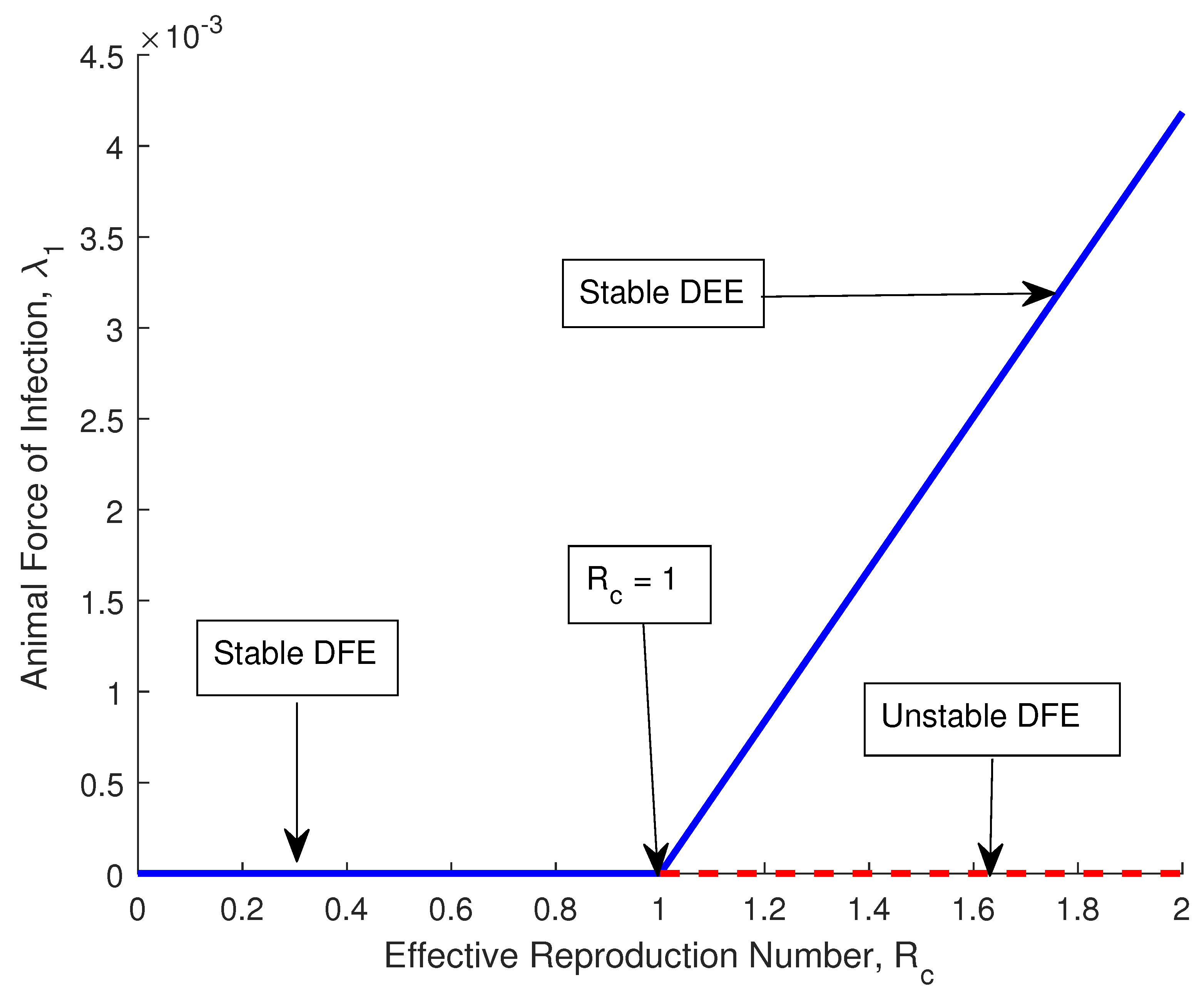
3.7. Bifurcation Analysis

Bifurcation analysis is the mathematical exploration of model dynamics (through its components/parameters) responsible for passing through a critical value or threshold (also known as a bifurcation point). Here, we investigate the model behavior under diverse scenarios using bifurcation analysis.

The model Equation (1) is rewritten as

$$\begin{array}{c}{f}_1=\frac{d{x}_1}{dt}=l_1-{\beta }_1(x_5+x_6)x_1-Q_0{x}_1+{\vartheta }_a{x}_4,\hfill \\ f_2=\frac{d{x}_2}{dt}=l_2+\theta x_1-{\mu }_a{x}_2,\hfill \\ f_3=\frac{d{x}_3}{dt}={\beta }_1(x_5+x_6)x_1-k_1{x}_3,\hfill \\ f_4=\frac{d{x}_4}{dt}={\gamma }_a{x}_3-l_0{x}_4,\hfill \\ f_5=\frac{d{x}_5}{dt}={\delta }_a{x}_3-k_2{x}_5,\hfill \\ f_6=\frac{d{x}_6}{dt}={\phi }_1{x}_3+{\phi }_2{x}_5-\xi x_6,\hfill \\ f_7=\frac{d{x}_7}{dt}=l_3-\chi x_7-{\beta }_2\left({\displaystyle \frac{x_3}{{\sum }_{i=1}^5{x}_i}}+x_5+x_6\right)x_7-{\mu }_h{x}_7+l_5{x}_{10},\hfill \\ f_8=\frac{d{x}_8}{dt}=l_4+\chi x_7-e{\beta }_2\left({\displaystyle \frac{x_3}{{\sum }_{i=1}^5{x}_i}}+x_5+x_6\right)x_8-{\mu }_h{x}_8+l_6{x}_{10},\hfill \\ f_9=\frac{d{x}_9}{dt}={\beta }_2\left({\displaystyle \frac{x_3}{{\sum }_{i=1}^5{x}_i}}+x_5+x_6\right)(x_7+e{x}_8)-k_3{x}_9,\hfill \\ f_{10}=\frac{d{x}_{10}}{dt}={\gamma }_h{x}_9-l_7{x}_{10},\hfill \end{array}$$

(14)

such that the state variables $S_a,V_a,I_a,R_a,C_a,P,S_h,S_l,I_h,R_h$ are replaced with $x_1,x_2,\cdots ,x_{10}$, respectively. The Jacobian matrix of (14) evaluated at disease-free equilibrium when ${\mathcal{R}}_c=1$ gives

$$J=\left[\begin{array}{cccccccccc}-Q_0& 0& 0& {\vartheta }_a& -\frac{{\beta }_1^{*}{l}_1}{Q_0}& -\frac{{\beta }_1^{*}{l}_1}{Q_0}& 0& 0& 0& 0\\ \theta & -{\mu }_a& 0& 0& 0& 0& 0& 0& 0& 0\\ 0& 0& -k_1& 0& \frac{{\beta }_1^{*}{l}_1}{Q_0}& \frac{{\beta }_1^{*}{l}_1}{Q_0}& 0& 0& 0& 0\\ 0& 0& {\gamma }_a& -l_0& 0& 0& 0& 0& 0& 0\\ 0& 0& {\delta }_a& 0& -k_2& 0& 0& 0& 0& 0\\ 0& 0& {\phi }_1& 0& {\phi }_2& -\xi & 0& 0& 0& 0\\ 0& 0& -\frac{{\beta }_2{\mu }_a{Q}_0{l}_3}{\left(\left(\theta +{\mu }_a\right)l_1+l_2{Q}_0\right)Q_1}& 0& -\frac{{\beta }_2{l}_3}{Q_1}& -\frac{{\beta }_2{l}_3}{Q_1}& -Q_1& 0& 0& l_5\\ 0& 0& -\frac{e{\beta }_2{\mu }_a{Q}_0\left(\chi l_3+l_4{Q}_1\right)}{{\mu }_h{Q}_1\left(\left(\theta +{\mu }_a\right)l_1+l_2{Q}_0\right)}& 0& -\frac{e{\beta }_2\left(\chi l_3+l_4{Q}_1\right)}{{\mu }_h{Q}_1}& -\frac{e{\beta }_2\left(\chi l_3+l_4{Q}_1\right)}{{\mu }_h{Q}_1}& \chi & -{\mu }_h& 0& l_6\\ 0& 0& \frac{{\beta }_2\left(\left(e\chi +{\mu }_h\right)l_3+e{Q}_1{l}_4\right){\mu }_a{Q}_0}{{\mu }_h{Q}_1\left(\left(\theta +{\mu }_a\right)l_1+l_2{Q}_0\right)}& 0& \frac{{\beta }_2\left(e\chi l_3+e{Q}_1{l}_4+l_3{\mu }_h\right)}{{\mu }_h{Q}_1}& \frac{{\beta }_2\left(e\chi l_3+e{Q}_1{l}_4+l_3{\mu }_h\right)}{{\mu }_h{Q}_1}& 0& 0& -k_3& 0\\ 0& 0& 0& 0& 0& 0& 0& 0& {\gamma }_h& -l_7\end{array}\right]$$

(15)

where ${\beta }_1^{*}={\displaystyle \frac{Q_0{k}_2{k}_1\xi }{l_1\left(\xi {\delta }_a+{\delta }_a{\phi }_2+k_2{\phi }_1\right)}}$.

Next, the left and right eigenvectors of (15) are obtained as $V=$$[v_1,v_2,v_3,v_4,v_5,v_6,v_7,v_8,v_9,v_{10}]$ and $W={[w_1,w_2,w_3,w_4,w_5,w_6,w_7,w_8,w_9,w_{10}]}^T$, where

$$\begin{array}{c}{v}_1=v_2=v_4=v_7=v_8=v_9=v_{10}=0,v_5=\frac{v_3{\beta }_1{l}_1\left(\xi +{\phi }_2\right)}{\xi Q_0{k}_2},v_6=\frac{v_3{\beta }_1{l}_1}{\xi Q_0},v_3>0\mathrm{free}\hfill \\ w_1=\frac{w_3\left(\xi Q_0{\gamma }_a{k}_2{\vartheta }_a-\xi {\beta }_1{\delta }_a{l}_0{l}_1-{\beta }_1{\delta }_a{l}_0{l}_1{\phi }_2-{\beta }_1{k}_2{l}_0{l}_1{\phi }_1\right)}{\xi {Q_0}^2{k}_2{l}_0},w_4=\frac{{\gamma }_a{w}_3}{l_0},w_6=\frac{w_3\left({\delta }_a{\phi }_2+k_2{\phi }_1\right)}{\xi k_2}\hfill \\ w_2=\frac{\theta w_3\left(\xi Q_0{\gamma }_a{k}_2{\vartheta }_a-\xi {\beta }_1{\delta }_a{l}_0{l}_1-{\beta }_1{\delta }_a{l}_0{l}_1{\phi }_2-{\beta }_1{k}_2{l}_0{l}_1{\phi }_1\right)}{\xi {Q_0}^2{k}_2{l}_0{\mu }_a},w_5=\frac{{\delta }_a{w}_3}{k_2},w_3>0\mathrm{free}\mathrm{and}\hfill \\ w_{i+6}\mathrm{free}\forall i=1,\dots ,4.\hfill \end{array}$$

(16)

Since $V·W=1$ gives $v_3\left(\left({\delta }_a{\phi }_2{k}_2+{\phi }_1{k_2}^2+\xi {\delta }_a\left(\xi +{\phi }_2\right)\right)l_1{\beta }_1+{\xi }^2{Q}_0{k_2}^2\right)w_3={\xi }^2{Q}_0{k_2}^2$, we therefore set $v_3={\displaystyle \frac{1}{v_3\left(\left({\delta }_a{\phi }_2{k}_2+{\phi }_1{k_2}^2+\xi {\delta }_a\left(\xi +{\phi }_2\right)\right)l_1{\beta }_1+{\xi }^2{Q}_0{k_2}^2\right)w_3}}$ and $w_3={\xi }^2{Q}_0{k_2}^2$. The non-zero second-order derivatives of (14) at disease-free equilibrium give

$$\begin{array}{c}{\displaystyle \frac{{\partial }^2{f}_1}{\partial x_1\partial x_5}}={\displaystyle \frac{{\partial }^2{f}_1}{\partial x_5\partial x_1}}={\displaystyle \frac{{\partial }^2{f}_1}{\partial x_1\partial x_6}}={\displaystyle \frac{{\partial }^2{f}_1}{\partial x_6\partial x_1}}=-{\beta }_1,\hfill \\ {\displaystyle \frac{{\partial }^2{f}_3}{\partial x_1\partial x_5}}={\displaystyle \frac{{\partial }^2{f}_3}{\partial x_5\partial x_1}}={\displaystyle \frac{{\partial }^2{f}_3}{\partial x_1\partial x_6}}={\displaystyle \frac{{\partial }^2{f}_3}{\partial x_6\partial x_1}}={\beta }_1,\hfill \\ {\displaystyle \frac{{\partial }^2{f}_7}{\partial x_1\partial x_3}}={\displaystyle \frac{{\partial }^2{f}_7}{\partial x_3\partial x_1}}={\displaystyle \frac{{\partial }^2{f}_7}{\partial x_1\partial x_7}}={\displaystyle \frac{{\partial }^2{f}_7}{\partial x_3\partial x_1}}=\frac{{\beta }_2{l}_3{{\mu }_a}^2{Q}_0}{\mathsf{\Omega }{Q}_1}.\hfill \end{array}$$

(17)

The substitution of (16) and (17) into $a={\sum }_{k,i,j=1}^{10}{v}_k{w}_i{w}_j{\displaystyle \frac{{\partial }^2{f}_k}{\partial x_i\partial x_j}}$ and $b={\sum }_{k,i=1}^{10}{v}_k{w}_i{\displaystyle \frac{{\partial }^2{f}_k}{\partial x_i\partial {\beta }_1}}$ yields

$$\begin{array}{c}a=-\frac{2{\beta }_1^{*}{v}_3{w_3}^2\left({\mu }_a\left(k_1+{\vartheta }_a\right)+{\delta }_a{\vartheta }_a\right)\left(\xi {\delta }_a+{\delta }_a{\phi }_2+k_2{\phi }_1\right)}{{\xi }^2{Q_0}^2{k_2}^2{l}_0}<0,\hfill \\ b=\frac{\left(\left(\xi +{\phi }_2\right){\delta }_a+k_2{\phi }_1\right)v_3{w}_3{l}_1}{\xi k_2{Q}_0}>0.\hfill \end{array}$$

(18)

Since $a<0$ and $b>0$, then by item (iv) of Theorem 2.2 in [6], the model (1) is said to exhibit forward bifurcation whenever $R_c=1$.

Figure 2 illustrates the dynamics of the proposed model about ${\mathcal{R}}_c$. When the effective reproduction number (${\mathcal{R}}_c$) lies between $[0,1)$, we say the anthrax DFE is locally asymptotically stable. For ${\mathcal{R}}_c>1$, then, the endemic equilibrium is stable. The interest of this subsection is to understand what happens when ${\mathcal{R}}_c=1$, and Figure 2 shows that the point of criticality for the stability of the disease is between DFE and disease-endemic equilibrium (DEE). Hence, the result:

Theorem 4.

The proposed model exhibits forward bifurcation at ${\mathcal{R}}_c=1$, and the model is stable.

3.8. Global Stability Analysis

Theorem 5.

The disease-free equilibrium is globally asymptotically stable whenever ${\mathcal{R}}_c\le 1$ and is unstable when ${\mathcal{R}}_c>1.$

Proof. 

The Lyapunov function Y shall be used to establish the global stability of (1) at disease-free equilibrium and is expressed as

$$Y={\displaystyle \frac{{\mathcal{R}}_c}{S_a^{+}}}{I}_a+{\displaystyle \frac{{\beta }_1\left\{\xi +{\phi }_2\right\}}{k_2\xi }}{C}_a+{\displaystyle \frac{{\beta }_1}{\xi }}P.$$

(19)

The time derivative of (19) gives

$$\dot{Y}={\displaystyle \frac{{\mathcal{R}}_c}{S_a^{+}}}\dot{I_a}+{\displaystyle \frac{{\beta }_1\left\{\xi +{\phi }_2\right\}}{k_2\xi }}\dot{C_a}+{\displaystyle \frac{{\beta }_1}{\xi }}\dot{P}.$$

(20)

Substitute the third, fifth, and sixth equation of the model in Equation (1) into the system (20) gives

$$\dot{Y}={\displaystyle \frac{{\mathcal{R}}_c}{S_a^{+}}}\left({\beta }_1\left(C_a+P\right)S_a-k_1{I}_a\right)+{\displaystyle \frac{{\beta }_1\left\{\xi +{\phi }_2\right\}}{k_2\xi }}\left({\delta }_a{I}_a+k_2{C}_a\right)+{\displaystyle \frac{{\beta }_1}{\xi }}\left({\phi }_1{I}_a+{\phi }_2{C}_a-\xi P\right).$$

(21)

Next, since $S_a\le S_a^{+}={\displaystyle \frac{l_1}{Q_0}}$, (21) gives

$$\dot{Y}\le \left({\mathcal{R}}_c{\beta }_1\left(C_a+P\right)-{\displaystyle \frac{R_c{k}_1}{S_a^{+}}}{I}_a\right)+{\displaystyle \frac{{\beta }_1\left\{\xi +{\phi }_2\right\}}{k_2\xi }}\left({\delta }_a{I}_a+k_2{C}_a\right)+{\displaystyle \frac{{\beta }_1}{\xi }}\left({\phi }_1{I}_a+{\phi }_2{C}_a-\xi P\right).$$

(22)

The simplification of (22) yields

$$\dot{Y}\le {\beta }_1\left(C_a+P\right)\left({\mathcal{R}}_c-1\right).$$

(23)

□

Theorem 6.

The endemic equilibrium (13) is globally asymptotically stable whenever ${\mathcal{R}}_c>1$ and is unstable otherwise.

The proof is presented in Appendix A.

4. Parameterization and Scenario Simulations

In this section, we present the parameter values (see

Table 2. Base values of parameters for simulation.

S/N	Parameter	Values	Source
1	${\beta }_1$	0.001–0.009	[25]
2	q	0.003	[24]
3	$\mathsf{\Omega }$	0.05	[25]
4	$\xi$	0.035	[25]
5	${\phi }_1$	0.45	[18,21]
6	${\delta }_a$	0.6	[22]
7	${\phi }_2$	0.001125	[22]
8	$\tau$	0.025	[25]
9	$\omega$	0.1	[17]
10	${\mu }_a$	0.0001	[18]
11	$\theta$	0.004	[24]
12	$\mathsf{\Pi }$	0.92	[18]
13	${\beta }_2$	0.0001	[8]
14	$\alpha$	0.6	Assumed
15	z	0.6	Assumed
16	${\varphi }_h$	0.6	[18]
17	$\chi$	[0, 0.9]	Assumed & [8]
18	${\gamma }_h$	0.04	[18]
19	${\mu }_h$	0.000042734	[27,28]
20	${\vartheta }_h$	0.5	[18]
21	${\vartheta }_a$	0.07	[24]
22	${\delta }_h$	0.02	[24]
23	${\gamma }_a$	0.0025	[18]

) used for the proposed model and simulate various scenarios. This numerical simulation is aimed at validating the qualitative analyses presented in the previous section.

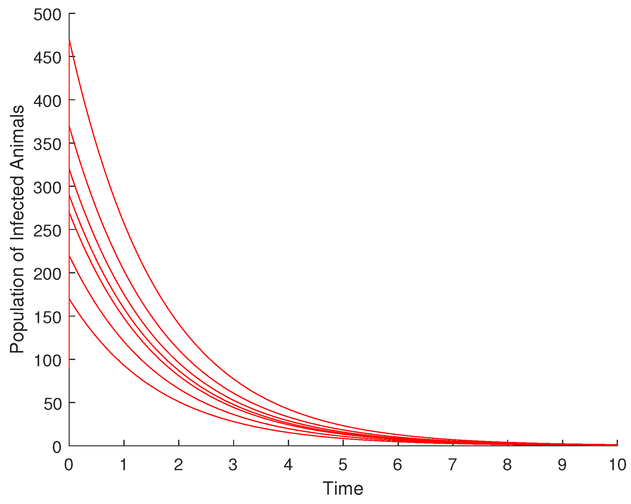
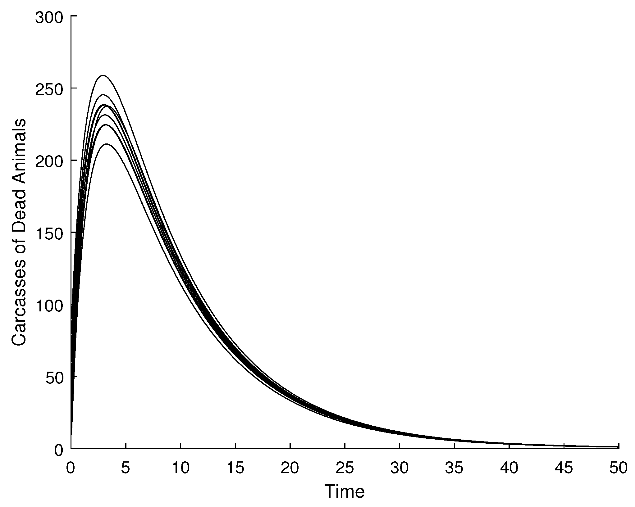
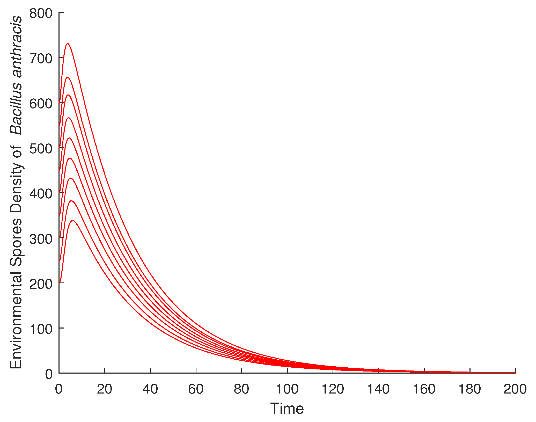
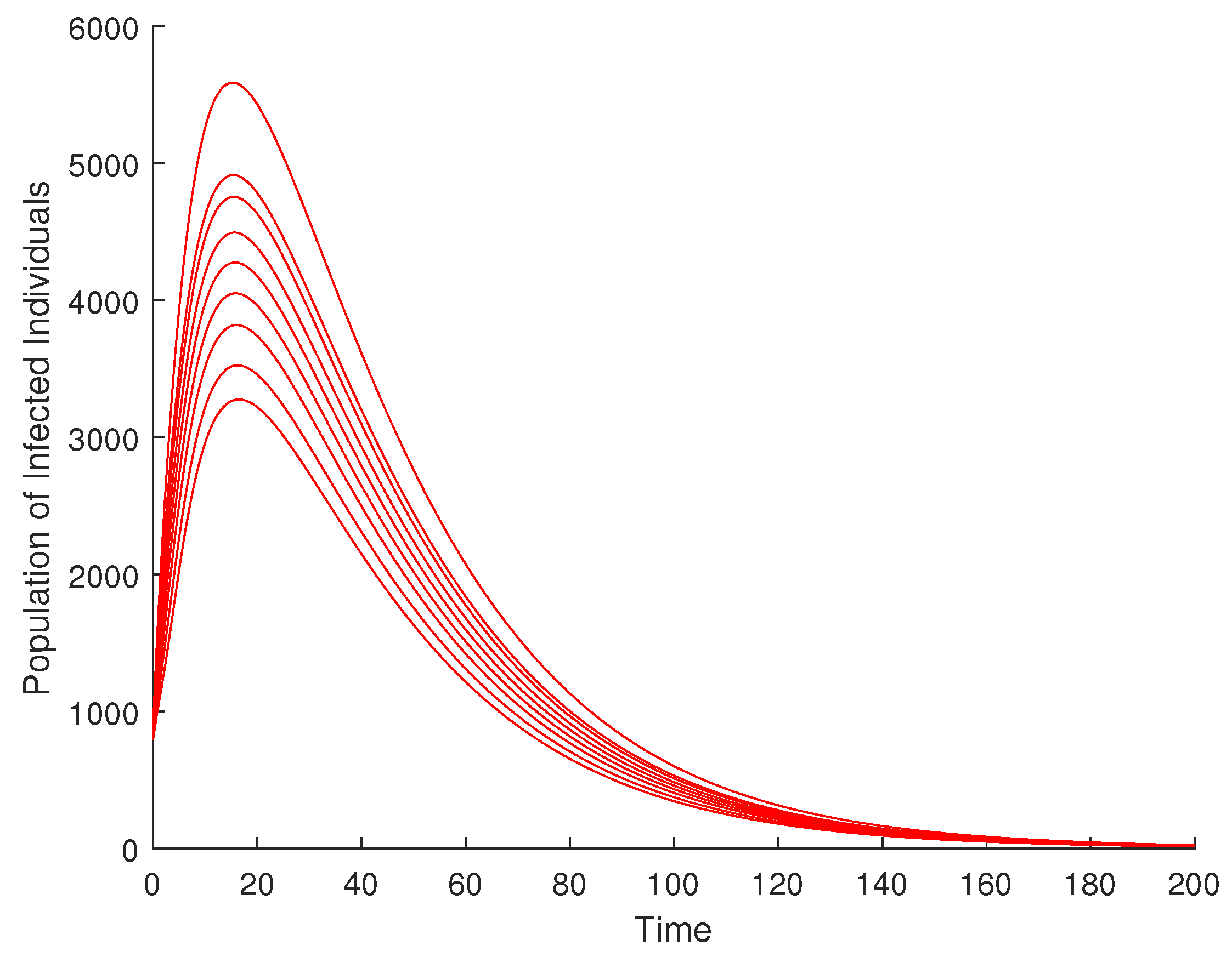
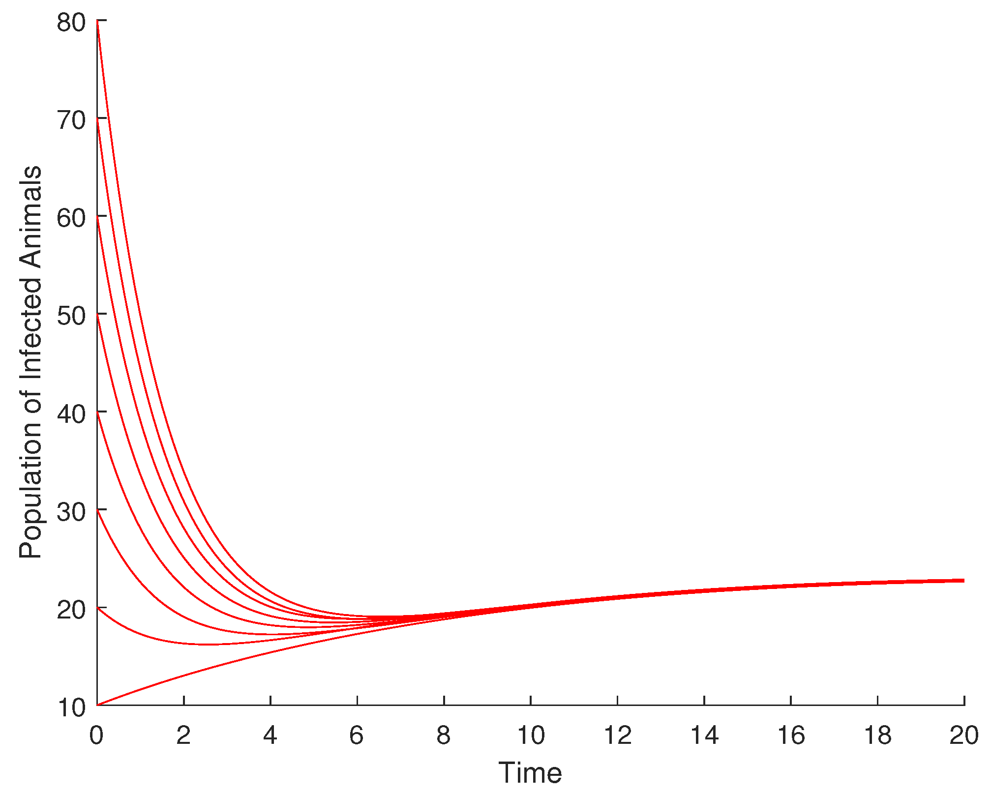
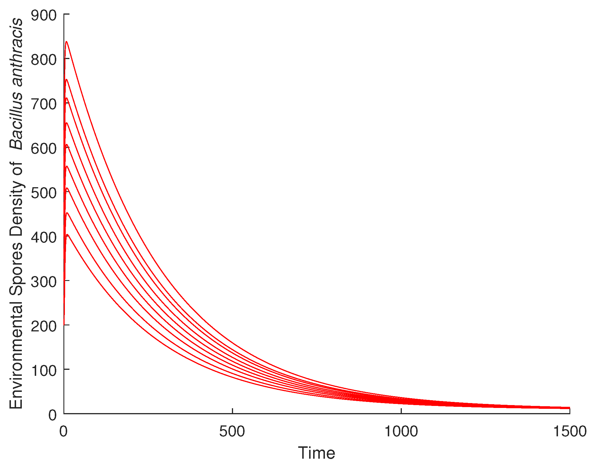
4.1. Validation of the Qualitative Analysis

From Figure 3, it is observed that the population of infected animals converges to zero (the DFE for the infected animal compartment) despite the variation in the initial conditions at disease-free equilibrium (DFE). Therefore, DFE is globally asymptotically stable for the infected animal compartment.

Figure 4 is the animal carcass compartment dynamics at DFE. This also converges to zero with the corresponding variation of the initial conditions. The same global asymptotic stability is observed for the environmental spore density of Bacillus anthracis, as shown in (Figure 5), and the infected human compartment, as illustrated in (Figure 6).

The global asymptotic stability simulation was performed at endemic equilibrium (EE) for various compartments, and the results are presented in Figure 7, Figure 8 and Figure 9. Simulation indicated that the global asymptotic stability of the endemic equilibrium point for the environmental spore density (Figure 10) would be achieved at about 1500 days, compared to the disease-free equilibrium, which converges in about 200 days (Figure 5).

While the carcass population at DFE is globally asymptotically stable at around zero in 50 days (Figure 4), the carcass population at EE was found to be globally stable at a point within the same 50 days (Figure 7).

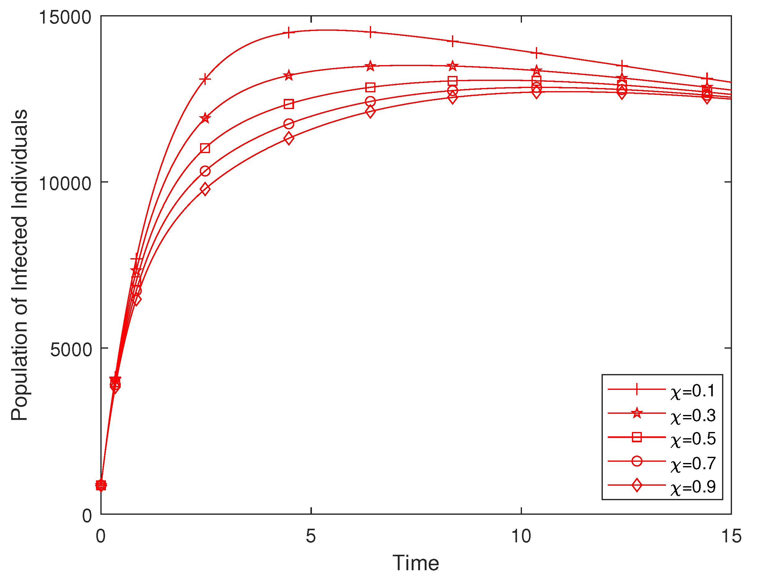
4.2. Effect of Enlightenment Campaign on the Disease Dynamics

Figure 11 presents a simulation investigating the impact of efforts at enlightening the human population $\chi$ in order to curtail disease incidence. It is observed that with an increase in the enlightenment effort, the population of infected individuals decreases significantly.

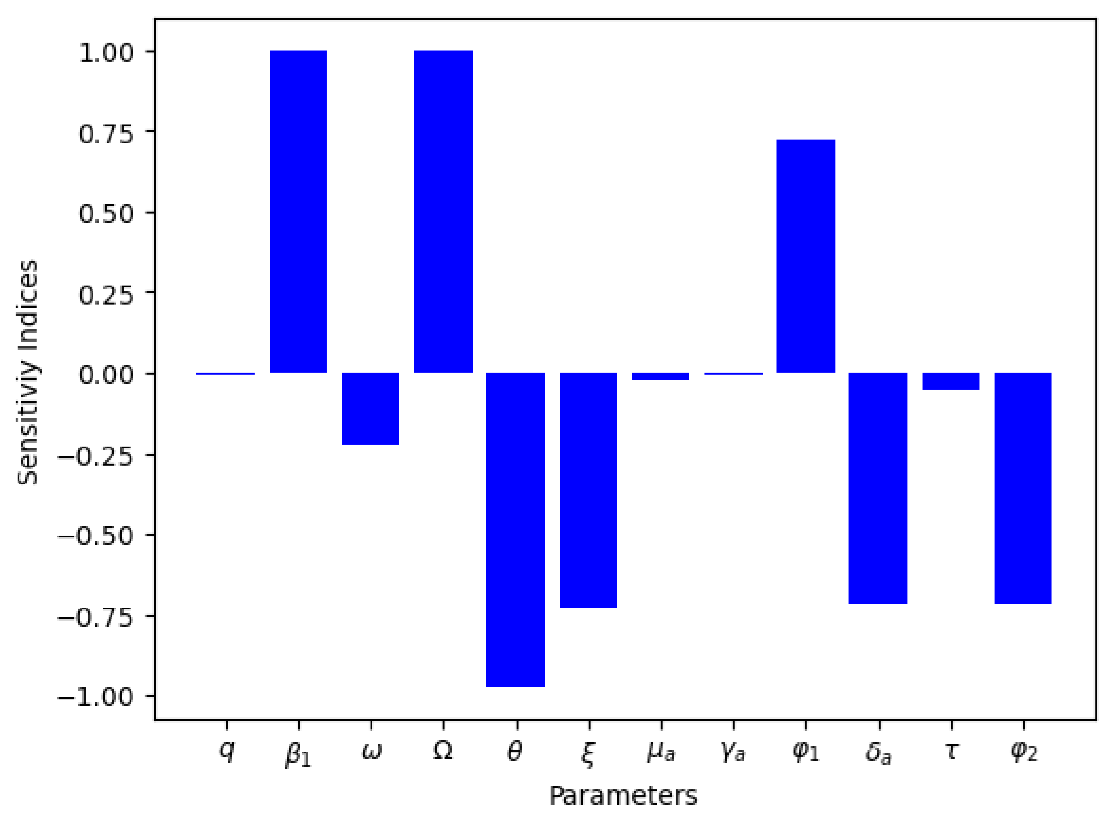
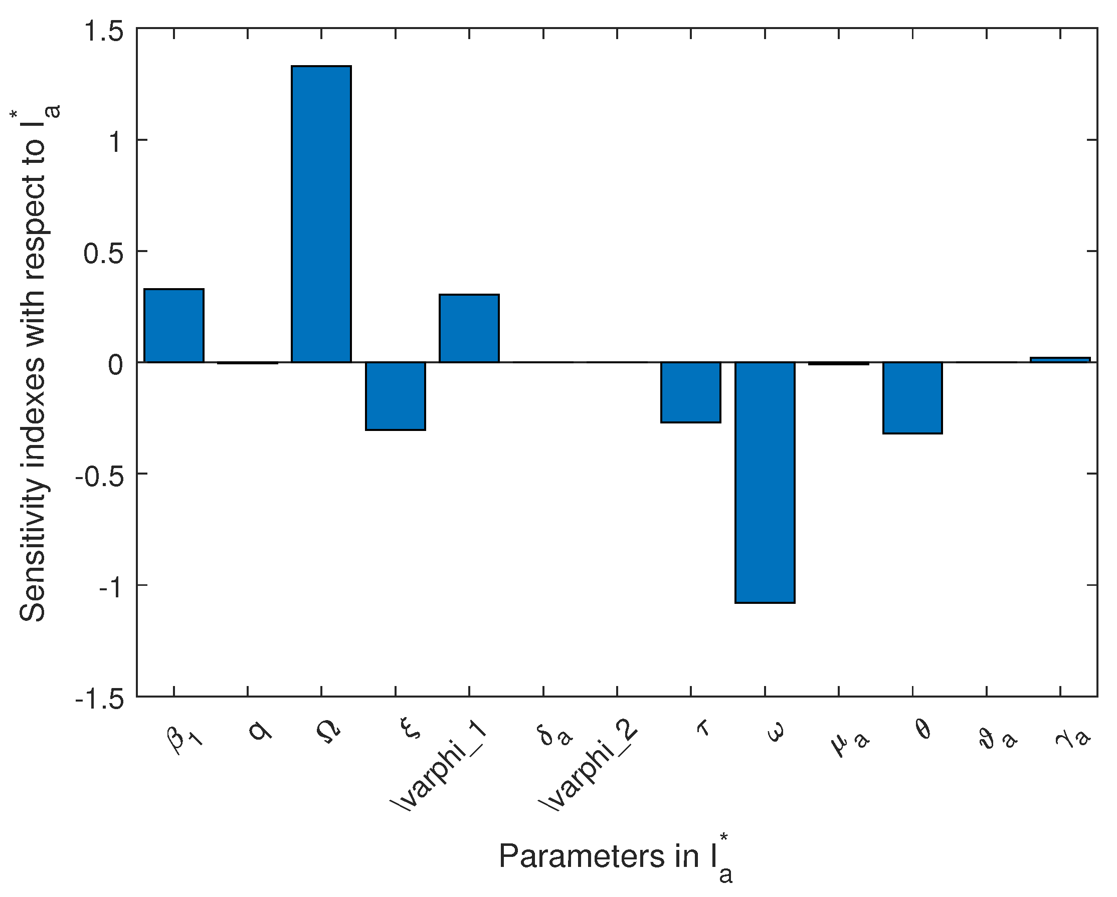
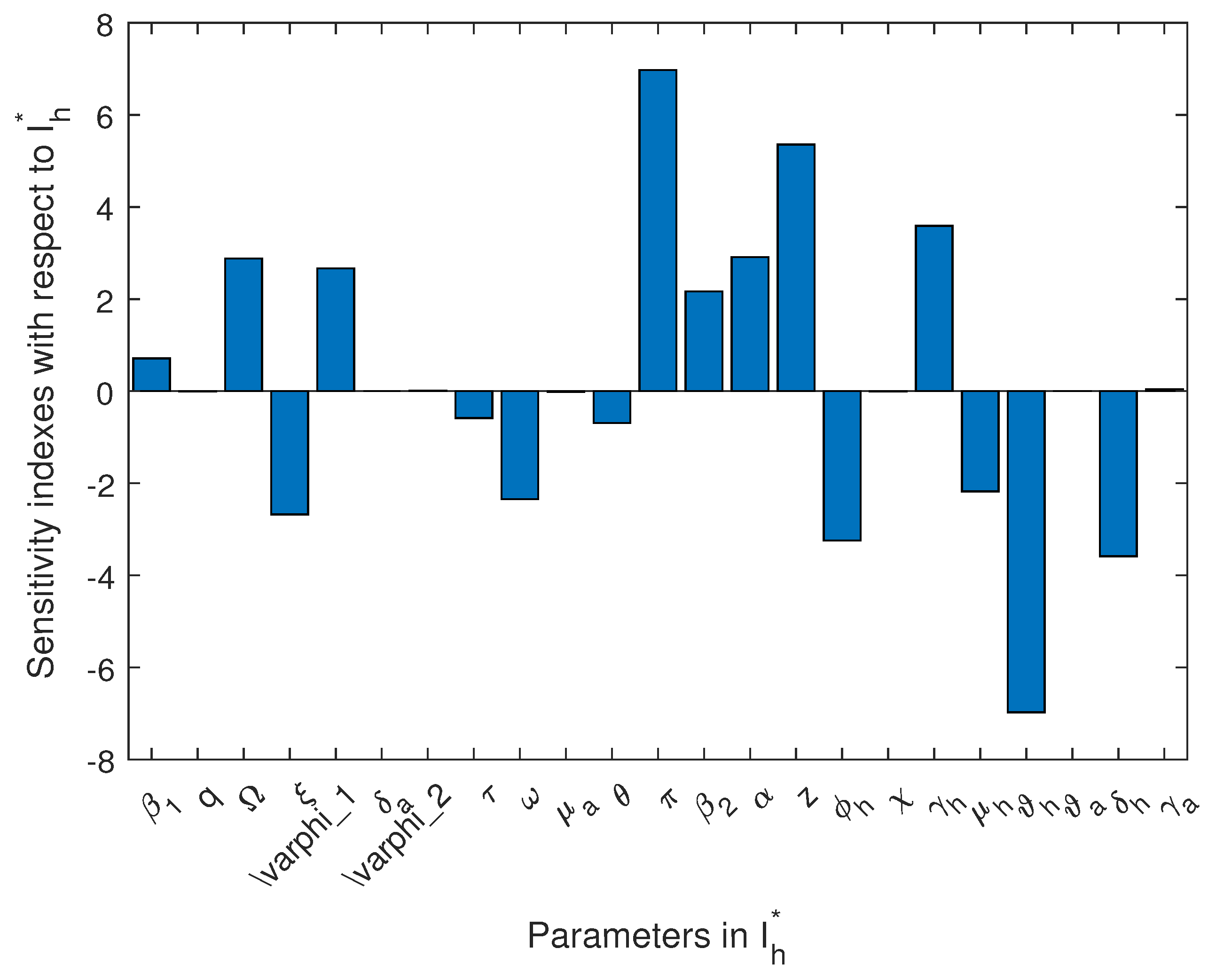
4.3. Sensitivity Analysis

In this section, we investigate the sensitivity indexes of the effective reproduction number with regard to its constituent parameters. This procedure can be seen in [8]. The sensitivity index of ${\mathcal{R}}_c$ with respect to the parameter y is given by

$${\gamma }_y^{{\mathcal{R}}_c}=\frac{y}{{\mathcal{R}}_c}·\frac{\partial {\mathcal{R}}_c}{\partial y}$$

for

$${\mathcal{R}}_c=\frac{\left(1-q\right)\mathsf{\Omega }\left(\left(\xi +{\phi }_2\right){\delta }_a+{\phi }_1\left(\tau +\omega \right)\right){\beta }_1}{\left({\mu }_a+\theta \right)\left({\gamma }_a+{\mu }_a+{\delta }_a\right)\left(\tau +\omega \right)\xi },$$

(24)

$${\gamma }_q^{{\mathcal{R}}_c}=-\frac{\mathsf{\Omega }\left(\omega {\phi }_1+\tau {\phi }_1+\xi {\delta }_a+{\delta }_a{\phi }_2\right){\beta }_1}{\left({\mu }_a+\theta \right)\left({\gamma }_a+{\mu }_a+{\delta }_a\right)\left(\tau +\omega \right)\xi },$$

$${\gamma }_{{\delta }_a}^{{\mathcal{R}}_c}=\frac{\left(1-q\right)\mathsf{\Omega }\left(\xi +{\phi }_2\right){\beta }_1}{\left({\mu }_a+\theta \right)\left({\gamma }_a+{\mu }_a+{\delta }_a\right)\left(\tau +\omega \right)\xi }-\frac{\left(1-q\right)\mathsf{\Omega }\left(\omega {\phi }_1+\tau {\phi }_1+\xi {\delta }_a+{\delta }_a{\phi }_2\right){\beta }_1}{\left({\mu }_a+\theta \right){\left({\gamma }_a+{\mu }_a+{\delta }_a\right)}^2\left(\tau +\omega \right)\xi },$$

$${\gamma }_{\xi }^{{\mathcal{R}}_c}=\frac{\left(1-q\right)\mathsf{\Omega }{\delta }_a{\beta }_1}{\left({\mu }_a+\theta \right)\left({\gamma }_a+{\mu }_a+{\delta }_a\right)\left(\tau +\omega \right)\xi }-\frac{\left(1-q\right)\mathsf{\Omega }\left(\omega {\phi }_1+\tau {\phi }_1+\xi {\delta }_a+{\delta }_a{\phi }_2\right){\beta }_1}{\left({\mu }_a+\theta \right)\left({\gamma }_a+{\mu }_a+{\delta }_a\right)\left(\tau +\omega \right){\xi }^2}.$$

In

Table 3. Normalized forward sensitivity index values for ${\mathcal{R}}_c$.

Parameter	Sensitivity Index
${\beta }_1$	1
q	−0.0030
$\mathsf{\Omega }$	1
$\xi$	−0.7305
${\phi }_1$	0.7218
${\phi }_2$	−0.7175
$\tau$	−0.0556
$\omega$	−0.2225
${\mu }_a$	−0.0246
${\gamma }_a$	−0.0041
${\delta }_a$	−0.7175
$\theta$	−0.9756

and Figure 12, we present the normalized forward sensitivity analysis result for ${\mathcal{R}}_c$. We can deduce that the effective disease transmission rate for animals (${\beta }_1$), pathogen release rate from infected animals (${\phi }_1$), and the recruitment rate into the animal population ($\mathsf{\Omega }$) are positively correlated to the effective reproduction number and are also statistically very significant in anthrax disease dynamics. Mitigation measure(s) that decrease these parameters will most definitely reduce the appearance of new infections in the population (both human and animal populations).

In

Table 4. Normalized forward sensitivity index values using the various indicated populations as response function at endemic equilibrium (${\mathcal{R}}_c=1.796887703>1$).

Par	${\mathit{S}}_{\mathit{a}}^{*}$	${\mathit{V}}_{\mathit{a}}^{*}$	${\mathit{I}}_{\mathit{a}}^{*}$	${\mathit{R}}_{\mathit{a}}^{*}$	${\mathit{C}}_{\mathit{a}}^{*}$	${\mathit{P}}^{*}$
${\beta }_1$	−0.9993	−0.9867	0.3280	0.3280	0.3286	0.3281
q	$-0.6003\times {10}^{-6}$	$-1.2343\times {10}^{-2}$	$-3.0999\times {10}^{-3}$	$-3.998\times {10}^{-3}$	$-3.998\times {10}^{-3}$	$-3.999\times {10}^{-3}$
$\mathsf{\Omega }$	$6.672\times {10}^4$	$1.277\times {10}^{-2}$	1.329	1.327	1.327	1.330
$\xi$	0.9275	0.9159	−0.3036	−0.3051	−0.3057	−1.304
${\phi }_1$	−0.9248	−0.9134	0.3036	0.3041	0.3029	1.301
${\phi }_2$	$2.304\times {10}^{-3}$	$2.276\times {10}^{-3}$	$7.530\times {10}^{-4}$	$7.555\times {10}^{-4}$	$7.559\times {10}^{-4}$	$3.236\times {10}^{-3}$
${\delta }_a$	$8.238\times {10}^{-6}$	$1.502\times {10}^{-5}$	$8.239\times {10}^{-6}$	$8.232\times {10}^{-6}$	$3.441\times {10}^{-3}$	$8.231\times {10}^{-6}$
$\tau$	0.1999	0.1973	−0.2697	−0.2695	$-2.698\times {10}^{-1}$	−0.2695
$\omega$	0.7996	0.7893	−1.079	−1.077	−1.080	−1.030
${\mu }_a$	$1.301\times {10}^{-5}$	−0.999	$-8.022\times {10}^{-3}$	$-9.440\times {10}^{-3}$	$-8.191\times {10}^{-3}$	$-8.022\times {10}^{-3}$
$\theta$	$4.116\times {10}^{-5}$	−0.9876	−0.3195	−0.3195	−0.3195	−0.3195
${\vartheta }_a$	$4.671\times {10}^{-4}$	0	$-6.854\times {10}^{-4}$	-0.9959	$2.296\times {10}^{-4}$	$8.859\times {10}^{-4}$
${\gamma }_a$	$3.180\times {10}^{-4}$	$3.144\times {10}^{-4}$	$2.030\times {10}^{-2}$	1.019	1.616	$2.028\times {10}^{-2}$

, we present the normal sensitivity index values for ${\mathcal{R}}_c=1.796887703>1$ using the various animal population compartments as response functions at endemic equilibrium, and in Figure 13, we present the visualization result for ${\mathcal{R}}_c=1.796887703>1$ for the endemicity (animal infected population).

In

Table 5. Normalized forward sensitivity index values using the various human population compartments as response functions at endemic equilibrium (${\mathcal{R}}_c=1.796887703>1$).

Par	${\mathit{S}}_{\mathit{h}}^{*}$	${\mathit{S}}_{\mathit{l}}^{*}$	${\mathit{I}}_{\mathit{h}}^{*}$	${\mathit{R}}_{\mathit{h}}^{*}$
${\beta }_1$	0.6474	0.3845	0.7137	0.7137
q	$-7.881\times {10}^{-3}$	$-4.684\times {10}^{-3}$	$-8.694\times {10}^{-3}$	$-8.694\times {10}^{-3}$
$\mathsf{\Omega }$	$2.611$	$1.550$	2.880	2.880
$\xi$	−2.427	−1.443	−2.679	−2.677
${\phi }_1$	2.418	1.436	2.666	2.665
${\phi }_2$	$6.008\times {10}^{-3}$	$3.565\times {10}^{-3}$	$6.623\times {10}^{-3}$	$6.623\times {10}^{-3}$
${\delta }_a$	$1.503\times {10}^{-5}$	$8.924\times {10}^{-6}$	$1.656\times {10}^{-5}$	$1.656\times {10}^{-5}$
$\tau$	−0.5314	−0.3157	−0.5858	−0.5853
$\omega$	−2.125	−1.263	−2.343	−2.343
${\mu }_a$	$-1.471\times {10}^{-2}$	$-8.737\times {10}^{-3}$	$-1.622\times {10}^{-2}$	$-1.622\times {10}^{-2}$
$\theta$	−0.6297	−0.3740	$-6.944\times {10}^{-1}$	$-6.944\times {10}^{-1}$
${\vartheta }_a$	$1.618\times {10}^{-3}$	$9.614\times {10}^{-4}$	$1.784\times {10}^{-3}$	$1.784\times {10}^{-3}$
${\gamma }_a$	$3.933\times {10}^{-2}$	$2.338\times {10}^{-2}$	$4.336\times {10}^{-2}$	$4.338\times {10}^{-2}$
${\delta }_h$	−3.257	−3.255	−3.588	−3.588
$\mathsf{\Pi }$	7.330	6.976	6.976	6.976
${\beta }_2$	1.968	1.168	2.169	2.168
$\alpha$	2.641	2.909	2.910	2.910
z	$5.628$	5.355	$5.361$	$5.355$
${\varphi }_h$	$-2.945$	$-1.746$	$-3.245$	$-3.245$
$\chi$	$-1.008$	$7.217\times {10}^{-3}$	$8.624\times {10}^{-3}$	$-8.014\times {10}^{-3}$
${\gamma }_h$	3.257	3.257	2.590	3.589
${\mu }_h$	$-1.976$	−2.176	−2.179	$-2.178$
${\vartheta }_h$	−6.329	−5.981	−5.981	−6.976

, we present the normal sensitivity index values for ${\mathcal{R}}_c=1.796887703>1$ for the endemicity (human population), and in Figure 14, we present the visualization result for ${\mathcal{R}}_c=1.796887703>1$ for the endemicity (human infected population). What we can deduce is that the effective disease transmission rate for animals and humans (${\beta }_1,{\beta }_2$), the rate of loss of infection-acquired immunity by animals (${\vartheta }_a$), the pathogen release rate from infected animals and decaying carcasses (${\phi }_1,{\phi }_2$), and the recruitment rate into animal and human populations ($\mathsf{\Omega },\mathsf{\Pi }$) are not negatively correlated to the basic reproduction number and that they are statistically significant. Therefore, mitigation measure(s) that decrease these parameters will most definitely reduce the appearance of new infections in the populations.

5. Conclusions

In conclusion, our study delves into the mathematical modeling of anthrax disease spread by employing epidemiological tools to gain insights into the dynamics of this zoonotic disease. Through our analyses, we present both qualitative and quantitative results that contribute to the understanding of anthrax transmission within animal and human populations.

We begin by developing a model to understand anthrax dynamics then present some mathematical analysis such as the boundedness, positivity, existence, and uniqueness of the model. We also present some equilibrium points of the model: that is, DFE and EE. The threshold parameter (${\mathcal{R}}_c$) of the model is obtained and examined using bifurcation theory. Our forward bifurcation analysis reveals a nuanced threshold behavior, indicating a qualitative change in the disease dynamics as ${\mathcal{R}}_c$ surpasses critical values. This knowledge is invaluable for informing strategies aimed at controlling and preventing anthrax outbreaks in both animal and human populations and how resources can be deployed for public health policy.

Furthermore, we present the global stability analysis of the equilibrium points, and the analytical results are validated with some scenarios simulation. We also establish the importance of an enlightenment campaign on disease dynamics. To determine the parameters that are relevant for reducing disease spread, we perform a normalized forward sensitivity analysis on ${\mathcal{R}}_c$. The analysis allows us to determine parameters for the effective reproduction number ${\mathcal{R}}_c$ for both populations and at the level of different compartments for animal populations and then human populations at endemic equilibrium.

Despite the advancements made in our study, certain limitations warrant acknowledgment. A significant constraint is the unavailability of robust data. Insufficient data hinders our ability to calibrate and validate the model, thus impacting the precision of parameter values used for model simulation of different scenarios to validate our qualitative analysis and further quantitatively analyze the developed model. This limitation underscores the challenges inherent in obtaining comprehensive datasets for infectious diseases with complex transmission patterns, like anthrax.

Addressing the limitations of our current study opens avenues for future research in modeling anthrax disease. To enhance the accuracy of our model predictions, efforts should be directed towards acquiring more extensive and high-quality data encompassing diverse geographical regions and host species. Additionally, incorporating real-time surveillance data can bolster the predictive power of the models, facilitating more reliable simulations of anthrax dynamics.

Future research endeavors could explore the integration of advanced statistical techniques and machine learning algorithms to handle uncertainties associated with parameter estimation and model predictions. Furthermore, investigating the impact of environmental factors such as climate and land use on anthrax transmission dynamics could contribute to a more holistic understanding of anthrax disease ecology. Another future work could use a meta-population model to examine the model at different spatial scales by incorporating mobility, which is an important driver of disease transmission.

We also intend, as an extension of this paper, to consider the maximum Lyapunov exponent (MLE) and analyze the time series for the model we developed in this article, which will enable us to determine the set of parameter values and initial conditions that will make the system chaotic. When these are obtained, the MLE will be solved and simulated numerically. Because the presence of a positive Lyapunov exponent implies that the system is chaotic, more than one implies that the system is hyperchaotic. Thus, the MLE will be used to determine whether the model system is chaotic.

In conclusion, our research lays the foundation for further investigations into anthrax disease modeling and emphasizes the importance of continuous data collection, model refinement, and multidisciplinary collaboration. By addressing these challenges and building on the insights gained, future research endeavors can contribute to the development of effective strategies for anthrax disease control and prevention.

References

1. Center for Disease Control (CDC). National Center for Emerging and Zoonotic Infectious Diseases (NCEZID), Division of High-Consequence Pathogens and Pathology (DHCPP). Available online: https://www.cdc.gov/anthrax/basics/index.html (accessed on 8 November 2023).
2. Doganay, M.; Metan, G.; Alp, E. A review of cutaneous anthrax and its outcome. J. Infect. Public Health 2010, 3, 98–105. [Google Scholar] [CrossRef]
3. Alam, M.E.; Kamal, M.M.; Moizur, R.; Aurangazeb, K.; Islam, M.S.; Hassan, J. Review of anthrax: A disease of farm animals. J. Adv. Vet. Anim. Res. 2022, 9, 323. [Google Scholar] [CrossRef] [PubMed]
4. World Health Organization; International Office of Epizootics. Anthrax in Humans and Animals; World Health Organization: Geneva, Switzerland, 2008. [Google Scholar]
5. Dragon, D.C.; Rennie, R.P. The ecology of anthrax spores: Tough but not invincible. Can. Vet. J. 1995, 36, 295–301. [Google Scholar] [PubMed]
6. Martcheva, M. Methods for deriving necessary and sufficient conditions for backward bifurcation. J. Biol. Dyn. 2019, 13, 538–566. [Google Scholar] [CrossRef] [PubMed]
7. World Health Organization (WHO). Available online: https://www.who.int/news-room/fact-sheets/detail/climate-change-and-health (accessed on 8 November 2023).
8. Baloba, E.B.; Seidu, B.; Bornaa, C.S.; Okyere, E. Optimal control and cost-effectiveness analysis of anthrax epidemic model. J. Inform. Med. Unlocked 2023, 42, 101355. [Google Scholar] [CrossRef]
9. Akinyemi, S.T.; Idisi, I.O.; Rabiu, M.; Okeowo, V.I.; Iheonu, N.; Dansu, E.J.; Abah, R.T.; Mogbojuri, O.A.; Audu, A.M.; Yahaya, M.M.; et al. A tale of two countries: Optimal control and cost-effectiveness analysis of monkeypox disease in Germany and Nigeria. Healthc. Anal. 2023, 2023, 100258. [Google Scholar] [CrossRef]
10. Iheonu, N.O.; Nwajeri, U.K.; Omame, A. A non-integer order model for Zika and Dengue co-dynamics with cross-enhancement. Healthc. Anal. 2023, 2023, 100276. [Google Scholar] [CrossRef]
11. Waku, J.; Oshinubi, K.; Adam, U.M.; Demongeot, J. Forecasting the Endemic/Epidemic Transition in COVID-19 in Some Countries: Influence of the Vaccination. Diseases 2023, 11, 135. [Google Scholar] [CrossRef] [PubMed]
12. Chen, X.; Bahl, P.; Silva, C.D.; Heslop, D.; Doolan, C.; Lim, S.; MacIntyre, C. Systematic Review and Evaluation of Mathematical Attack Models of Human Inhalational Anthrax for Supporting Public Health Decision Making and Response. Prehospital Disaster Med. 2020, 35, 412–419. [Google Scholar] [CrossRef]
13. Mushayabasa, S.; Marijani, T.; Masocha, M. Dynamical analysis and control strategies in modeling anthrax. Comp. Appl. Math. 2017, 36, 1333–1348. [Google Scholar] [CrossRef]
14. Saad-Roy, C.M.; Driessche, P.v.; Yakubu, A.A. A Mathematical Model of Anthrax Transmission in Animal Populations. Bull. Math. Biol. 2017, 79, 303–324. [Google Scholar] [CrossRef] [PubMed]
15. Otieno, F.T.; Gachohi, J.; Gikuma-Njuru, P.; Kariuki, P.; Oyas, H.; Canfield, S.A.; Bett, B.; Njenga, M.K.; Blackburn, J.K. Modeling the Potential Future Distribution of Anthrax Outbreaks under Multiple Climate Change Scenarios for Kenya. Int. J. Environ. Res. Public Health 2021, 18, 4176. [Google Scholar] [CrossRef] [PubMed]
16. Osman, S.; Makinde, O.D.; Theuri, D.M. Mathematical modeling of Transmission Dynamics of Anthrax in Human and Animal Population. Math. Theory Model. 2018, 8, 201847. [Google Scholar]
17. Raza, A.; Baleanu, D.; Yousaf, M.; Akhter, N.; Mahmood, S.K.; Rafiq, M. Modeling of Anthrax Disease via Efficient Computing Techniques. Intell. Autom. Soft Comput. (IASC) 2022, 32, 1109–1124. [Google Scholar] [CrossRef]
18. Baloba, E.B.; Seidu, B. A Mathematical Model of Anthrax Epidemic with Behavioural Change. J. Math. Model. Control. (MMC) AIMS 2022, 2, 243–256. [Google Scholar] [CrossRef]
19. Gomez, J.P.; Nekorchuk, D.M.; Mao, L.; Ryan, S.J.; Ponciano, J.M.; Blackburn, J.K. Decoupling Environmental Effects and Host Population Dynamics for Anthrax, a Classic Reservoir-Driven Disease. PLoS ONE 2018, 13, e0208621. [Google Scholar] [CrossRef] [PubMed]
20. Kashyap, A.J.; Bordoloi, A.J.; Mohan, F.; Devi, A. Dynamical Analysis of an Anthrax Disease Model in Animals with Nonlinear Transmission. Math. Model. Control. 2023, 3, 370–386. [Google Scholar] [CrossRef]
21. Efraim, J.E.; Irunde, J.I.; Kuznetsov, D. Modeling the Transmission Dynamics of Anthrax Disease in Cattle and Humans. J. Math. Comput. Sci. 2018, 8, 654–672. [Google Scholar] [CrossRef]
22. Zerihun, M.S.; Narasimha, M.S. Modeling and Simulation Study of Anthrax Attack On Environment. J. Multidiscip. Eng. Sci. Technol. (JMEST) 2016, 3, 4574–4578. [Google Scholar]
23. Denekew, Z.A.; Sunita, G.; Kumar, G.S. Model for Transmission and Optimal Control of Anthrax Involving Human and Animal Population. J. Biol. Syst. 2022, 30, 605–630. [Google Scholar] [CrossRef]
24. Prawandani, N.; Toaha, S.; Kasbawati, S. VSEIR Mathematical Model on Anthrax Disease Dissemination in Animal Population with Vaccination and Treatment Effects. J. Mat. Stat. Komputari 2020, 17, 14–25. [Google Scholar] [CrossRef]
25. Alfwzan, W.F.; Abuasbe, K.; Raza, A.; Rafiq, M.; Awadalla, M.; Almulla, M.A. A Non-standard Computational Method for Stochastic Anthrax Epidemic Model. AIP Adv. 2023, 3, 075022. [Google Scholar] [CrossRef]
26. Den Driessche, P.V.; Watmough, J. Reproduction numbers and sub-threshold endemic equilibria for compartmental models of disease transmission. Math. Biosci. 2002, 180, 29–48. [Google Scholar] [CrossRef] [PubMed]
27. Data from United Nations. 2023. Available online: https://population.un.org/wpp/Download/Standard/MostUsed (accessed on 8 November 2023).
28. Macrotrends. Africa Life Expectancy 1950–2023. Available online: https://www.macrotrends.net/countries/AFR/africa/life-expectancy#:~:text=The%20life%20expectancy%20for%20Africa,a%200.46%25%20increase%20from%202019 (accessed on 8 November 2023).
29. La Salle, J.P. The stability of dynamical systems. In Society of Industrial and Applied Mathematics—SIAM; E-book: Rijeka, Croatia, 1976. [Google Scholar]
Figure 1. Schematic diagram of Anthrax model (1).
Mathematics 12 01014 g001
Figure 2. Forward bifurcation plot.
Mathematics 12 01014 g002
Figure 3. Diagram illustrating the global asymptotic stability of DFE for the infected animal population.
Mathematics 12 01014 g003
Figure 4. Visualization of global asymptotic stability of DFE for the animal carcass compartment.
Mathematics 12 01014 g004
Figure 5. Global asymptotic stability of DFE for the environmental spores.
Mathematics 12 01014 g005
Figure 6. Global asymptotic stability of DFE for the infected human compartment.
Mathematics 12 01014 g006
Figure 7. GAS of the endemic equilibrium for the carcasses.
Mathematics 12 01014 g007
Figure 8. Global asymptotic stability of endemic equilibrium for infected animals.
Mathematics 12 01014 g008
Figure 9. Global stability of endemic equilibrium for infected humans.
Mathematics 12 01014 g009
Figure 10. Global asymptotic stability of endemic equilibrium for spore density.
Mathematics 12 01014 g010
Figure 11. Variation of efforts for the enlightenment of the populace.
Mathematics 12 01014 g011
Figure 12. Normalized forward sensitivity analysis result visualization for R c .
Mathematics 12 01014 g012
Figure 13. Sensitivity index using animal infected compartment as response function at endemicity.
Mathematics 12 01014 g013
Figure 14. Sensitivity index using the human infected compartment at endemic equilibrium as the response function.
Mathematics 12 01014 g014